An explainable digital twin framework for skin cancer analysis using early activation meta-learner

Skin cancer is among the most common cancers globally, which calls for timely and precise diagnosis for successful therapy. Conventional methods of diagnosis, including dermoscopy and histopathology, are significantly dependent on expert judgment and therefore are time-consuming and susceptible to inconsistencies. Deep learning algorithms have shown potential in skin cancer classification but tend to consume a substantial amount of computational resources and large training sets. To overcome these issues, we introduce a new hybrid computer-aided diagnosis (CAD) system that integrates Stem Block for feature extraction and machine learning for classification. The International Skin Imaging Collaboration (ISIC) skin cancer dermoscopic images were collected from Kaggle, and essential features were collected from the Stem Block of a deep learning (DL) algorithm. The selected features, which were standardized using StandardScaler to achieve zero mean and unit variance, were then classified using a meta-learning classifier to enhance precision and efficiency. In addition, a digital twin framework was introduced to simulate and analyze the diagnostic process virtually, enabling real-time feedback and performance monitoring. This virtual replication aids in continuous improvement and supports the deployment of the CAD system in clinical environments. To improve transparency and clinical reliability, explainable artificial intelligence (XAI) methods were incorporated to visualize and interpret model predictions. Compared to state-of-the-art approaches, our system reduced training complexities without compromising high classification precision. Our proposed model attained an accuracy level of 96.25%, demonstrating its consistency and computationally efficient status as a screening tool for detecting skin cancer.

1 Introduction

Skin cancer is one of the most widespread and serious health conditions globally, affecting millions of people annually. The skin is the largest human body organ, and it serves very important functions such as protecting against external elements, controlling temperature, and preventing excessive water loss. Due to its prolonged exposure to ultraviolet (UV) light, harmful environmental factors, and hereditary tendencies, the skin is susceptible to cancer. Skin cancer occurs when the skin cells grow abnormally and uncontrollably, usually because of extensive exposure to UV light (Melarkode et al., 2023).

The World Health Organization (WHO) states that skin cancer is responsible for one-third of all cancers worldwide, and melanoma is the deadliest and most malignant type (Brancaccio et al., 2024). Non-melanoma skin cancer (NMSC) accounts for an estimated 2 to 3 million cases annually, while melanoma recorded approximately 330,000 new cases and 60,000 deaths globally in 2022. The incidence of skin cancer is notably higher in regions such as Oceania, North America, and Europe (Wang et al., 2025). Australia reports rates 10 to 20 times higher than those in European populations. Melanoma has a five-year survival rate of 99.6% when diagnosed at an early stage, and delayed diagnosis markedly decreases survival rates, indicating the importance of early and correct detection techniques (Salinas et al., 2024).

Conventional skin cancer diagnosis is mainly based on dermatological inspection, dermoscopy, and histopathological examination (Naqvi et al., 2023). Dermoscopy is a painless imaging method that facilitates visualization of structures beneath the surface of lesions that are invisible to the naked eye, contributing to a high diagnostic precision (Wei et al., 2024). The reliability of dermoscopy is highly dependent on the dermatologist, making it vulnerable to inter-observer variation (Akter et al., 2025). Histopathological examination, the gold standard for skin cancer diagnosis, entails tissue biopsy followed by microscopic examination, but it is time-consuming, expensive, and invasive (Tai et al., 2024). Consequently, the need for faster, objective, and automated diagnostic tools has grown in recent times (Claret et al., 2024). With the recent advancements in artificial intelligence (AI) and deep learning (DL), computer-aided diagnosis (CAD) systems have proven to be efficient tools for detecting skin cancer (Mahmud et al., 2023).

Convolutional neural networks (CNNs) have achieved outstanding performance in automatically detecting hierarchical features of dermoscopic images to perform accurate skin lesion classification (Himel et al., 2024). Traditional end-to-end deep models are computationally demanding, requiring large labeled datasets, time-consuming training procedures, and vast computational power, which, in practical terms, seems to be not feasible in real-world settings (Thompson et al., 2020). Features with high dimensionality in a single CNN layer can complicate the classification task and result in overfitting, thus weakening the generalizability of models (Georgiou et al., 2020).

Many deep learning models have been developed to classify skin cancer; however, most of the current approaches have inherent limitations, which include concerns regarding excessive computational cost, overfitting due to limited training data, and lack of interpretability. In addition, traditional end-to-end classification models usually fail to take advantage of the complementary benefits of multiple learning methods. Our research addresses these limitations through a hybrid framework that employs deep feature extraction using a lightweight pre-trained model combined with a meta-learning-based stacking classifier. Unlike previous studies, our proposed framework takes into account the need for efficient feature selection, better generalization, and model interpretability in a skin cancer classification system designed for real-world clinical applications, where computing power and labeled data may be limited.

In view of these challenges, this study innovatively developed a new hybrid CAD system for the diagnosis of skin cancer that combines feature extraction from deep learning and machine learning-based classification.

• The proposed approach utilizes a pre-trained deep learning model to extract high-level features from dermoscopic images for skin cancer classification.

• Instead of using all deep features indiscriminately, t-distributed stochastic neighbor embedding (t-SNE) visualization is employed to identify the most relevant and informative layers, enabling effective and selective feature extraction.

• This feature selection strategy reduces redundancy and retains only the most discriminative representations of skin lesions, improving model efficiency.

• The selected deep features are input into a meta-learning classifier, which effectively handles high-dimensional data and enhances classification performance.

• The primary contribution is the development of a novel hybrid diagnostic framework that combines early activation deep feature extraction with meta-learning classification.

• The methodology emphasizes the use of t-SNE-based layer selection to identify the most learnable layers in the early activation block of the model, ensuring optimal feature input.

• By avoiding the use of all model layers, the approach significantly reduces computational complexity and training time without compromising accuracy.

• The integration of a meta-learning classifier improves diagnostic accuracy when compared to traditional end-to-end deep learning models.

• A digital Twin of the diagnostic system is conceptualized to simulate the end-to-end diagnostic workflow, enabling iterative testing, real-time monitoring, and safe validation before clinical deployment.

• To support clinical trust and transparency, the framework incorporates explainable AI (XAI) techniques (e.g., Grad-CAM, saliency maps) to visually interpret model decisions and highlight key image regions influencing classification outcomes.

2 Materials and methods

2.1 Related works

Table 1 is a comparative overview of different deep learning and hybrid approaches utilized in recent research for skin lesion classification. The table summarizes each method's accuracy and its limitations. It is an exhaustive overview of available approaches based on model performance and complexity. This overview assists in determining the gaps and challenges that still exist in the field, including low performance, high complexity, and dependence on a single model type.

Table 1

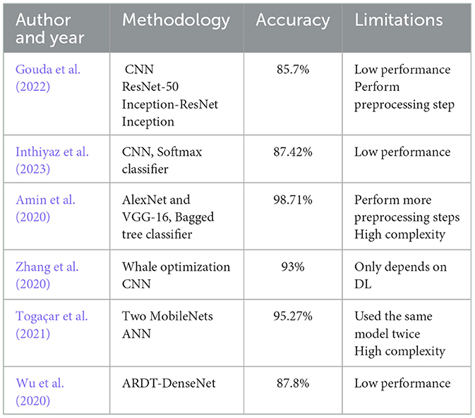
Table 1. Literature review.

Deep learning algorithms are commonly employed for the extraction of intricate features from dermoscopic images, with research achieving accuracies of 98.75% using sophisticated feature extraction methods such as local optimal-oriented pattern (LOOP) and gray-level co-occurrence matrix (GLCM) (Alharbi et al., 2024). Hybrid systems that combine deep learning and machine learning classifiers have also shown promising results such as DenseNet201 with support vector machines (SVMs), which registered 91.09% accuracy on the International Skin Imaging Collaboration (ISIC) dataset. Transfer learning methodologies with pre-trained models such as EfficientNet-B7 and ResNet50 have also improved performance, with EfficientNet-B7 recording 84.4% accuracy (Kanchana et al., 2024). To overcome shortcomings such as computational inefficiency and large dataset requirement, a novel hybrid CAD system has been proposed, comprising a Stem Block for feature extraction and a meta-learning classifier for classification. The Stem Block identifies key features from dermoscopic images through deep learning algorithms, and the meta-learning classifier promotes accuracy by basing its approach on knowledge generalization across different datasets. A comparative evaluation was conducted between direct classification using the MobileNetV2 model and the proposed hybrid approach. In the direct classification setup, MobileNetV2 achieved an accuracy of 90.00%, whereas the proposed approach demonstrated a significant improvement with an accuracy of 96.25%. This enhancement can be attributed to the use of refined deep features and the ability of the meta-learning classifier to effectively combine multiple learners for better generalization. This model exhibited a high accuracy of 96.25%, with decreased training complexities, rendering it appropriate for real-time clinical use. In comparison to current state-of-the-art models, the proposed model performs better while being computationally efficient.

2.2 Methodology

During the implementation of the proposed hybrid CAD framework, several technical challenges were addressed to ensure optimal performance. One major challenge was the selection of meaningful deep features from the pre-trained MobileNetV2 model. Using all feature maps without evaluating their relevance led to increased computational cost and a higher risk of overfitting. To resolve this, t-SNE-based analysis was applied to identify and retain only the most discriminative layers, allowing the model to focus on high-impact features. Another key consideration was the design and tuning of the stacking classifier, where multiple base learners were integrated. It was essential to carefully validate these learners to ensure that they provided complementary decision boundaries without redundancy. The hyperparameters of both the base learners and the meta-classifier were fine-tuned through empirical testing to achieve optimal balance and performance. These methodological choices contributed to the overall robustness, efficiency, and high accuracy of the proposed hybrid model in skin cancer classification. Figure 1 shows the overall architecture diagram for the proposed model.

Figure 1

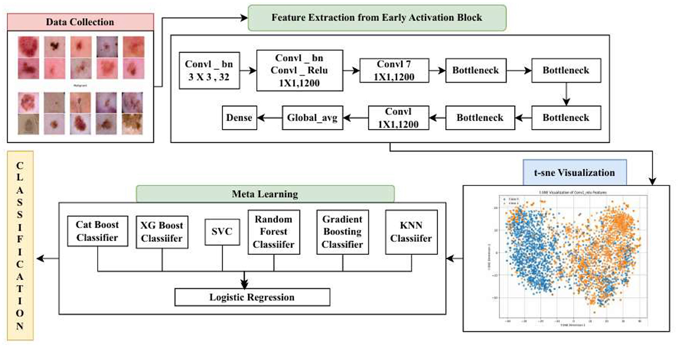
Figure 1. Work flow of the proposed model.

2.2.1 Dataset description

This section describes the benchmark dataset used to evaluate the performance of the proposed model. The skin lesion images are part of the dataset, and they are downloadable from the International Skin Imaging Collaboration (ISIC) repository. The dataset contains two classes: malignant and benign tumors, along with respective image annotations provided by medical doctors who performed biopsies to diagnose them. Dermoscopy imaging was performed to better visualize tumor structures. The dataset contains 3,297 images, of which 1,800 are benign and 1,497 are malignant. The dataset is publicly available on Kaggle. Figure 2 displays some sample images from the malignant class, and Figure 3 displays some sample images from the benign class. The images are scaled down to 224 × 224 pixels.

Figure 2

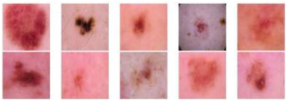
Figure 2. Skin cancer: malignant.

Figure 3

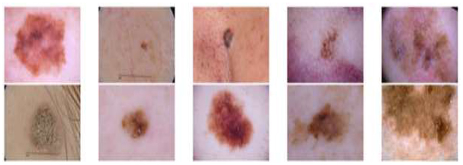
Figure 3. Skin cancer: benign.

2.2.2 Early activation block

The Stem Block serves as the foundational feature extractor, as shown in Figure 4. It processes input images into a lower-resolution, high-channel representation suitable for subsequent layers (Sandler et al., 2018). The Stem Block consists of an initial 3 × 3 convolution with a stride of 2, followed by batch normalization and a ReLU6 activation, forming the conv1_relu layer (Zhu et al., 2024).

Figure 4

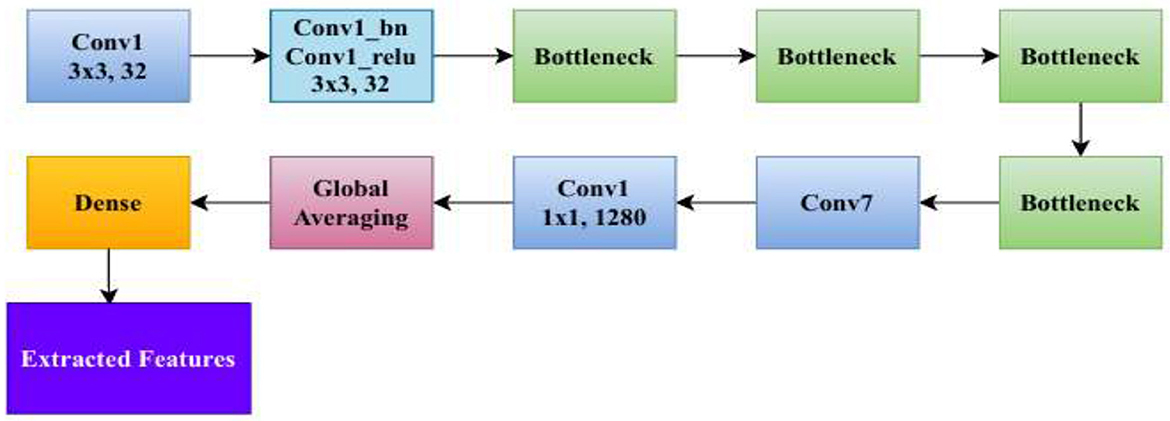
Figure 4. Architecture of the deep learning model used.

Depthwise separable convolution is a computationally efficient alternative to regular convolution and is utilized extensively in lightweight neural network frameworks. As opposed to conventional convolution where the same convolution filter is applied for all input channels, it performs the operation in two distinct steps: depthwise convolution and pointwise convolution. This considerably alleviates the cost of computation and improves model efficiency without significantly degrading performance. In the depthwise convolution process, one filter is applied to each input channel independently, instead of summing up all channels together using several filters. Equation 1 represents the formula for the computational cost of depthwise convolution, where h is the height of the input feature map, w is the width of the input feature map, c is the number of input channels, and k is the size of the convolutional kernel.

$\begin{array}{ll}CostDepthwise=h\times w\times c\times k^2& (1)\end{array}$

Equation 2 represents the computational cost of pointwise convolution. In pointwise convolution, 1 × 1 convolutions are employed to fuse the features of all channels, effectively combining channel information. Here, d is the number of output channels.

$\begin{array}{ll}CostPointwise=h\times w\times c\times d& (2)\end{array}$

Equation 3 represents the overall computational cost of depthwise separable convolution, which is the sum of the depthwise and pointwise convolution costs.

$\begin{array}{ll}TotalCost=h\times w\times c\times \left(k^2+d\right)& (3)\end{array}$

One of the key reasons for choosing the Stem Block is its complexity vs. performance trade-off. The architecture is tailored to improve feature representation through linear bottlenecks and expansion layers such that it can learn rich spatial and channel-wise information efficiently. While it is lightweight, it has been demonstrated to produce excellent classification accuracy on large-scale databases such as ImageNet, where it outperforms the majority of conventional architectures based on an efficiency-to-performance ratio.

Equation 4 represents the structure of an inverted residual block, where the input x is initially subjected to a 1 × 1 convolution to increase the number of channels, followed by a 3 × 3 depthwise convolution, then compressed using another 1 × 1 convolution. Linear activation occurs before residual connection addition. This design assists in maintaining the input while facilitating economical feature transformation at lower computational expense. In addition, it has also proven to be highly suitable for medical image classification tasks, such as the ISIC skin cancer dataset employed in this study (Surya et al., 2023).

$\begin{array}{ll}B(x)=x+Linear(Con{v}_{1x1}\left(DepthwiseCon{v}_{3x3}\left(Con{v}_{1x1}\left(x\right)\right)\right)& (4)\end{array}$

The expansion layer is a key component in the architecture of deep learning models. Its purpose is to expand the number of channels before applying depthwise convolution. This operation allows the network to learn richer and more complex feature representations. The expansion layer increases the number of channels by a factor t, which is set to 6. The input channels C_in are multiplied by this factor to produce a higher-dimensional intermediate representation known as the hidden channels C_hidden. Equation 5 represents the number of channels after expansion. It captures finer details and richer spatial features.

$\begin{array}{ll}{C}_{hidden}=t\times C_{in}=6C_{in}& (5)\end{array}$

Medical imaging demands models that effectively extract relevant patterns at a computationally reasonable cost, particularly with big datasets. Its low-cost feature extraction mechanism (Sawal and Kathait, 2023) makes it a very good fit for transfer learning. This guarantees that the model retains richer feature representations along with fitting itself to the sensitivities of medical image classification (Tika Adilah and Kristiyanti, 2023). In comparison with heavyweight architectures, it provides equivalent classification accuracy but with much reduced computational requirements, which makes it a perfect fit for large-scale processing. In addition, its strong ability to generalize well across different tasks and datasets aligns with the scope of this study, where accurate and efficient classification of images of skin cancer is of high importance (Ragab et al., 2022). Due to the advantage of its lightweight design, powerful feature extraction ability, high efficiency, and excellent performance in medical image processing, it is a perfect model for this research (Ekmekyapar and Taşci, 2023). Its computation cost at the expense of meaningful feature extraction makes it perfect for skin lesion classification, finally improving diagnostic accuracy and clinical decision-making (Xu and Mohammadi, 2024).

2.2.3 Feature extraction

In this study, we used t-SNE to identify the most learnable feature representations from the model's intermediate layers. t-SNE is a non-linear dimensionality reduction method that maintains local structures in high-dimensional data by probabilistic similarity matching (Van der Maaten and Hinton, 2008). t-SNE first computes pairwise similarities between high-dimensional feature vectors. For two features f_i and f_j from a layer l, it calculates how similar they are using a Gaussian kernel. Equation 6 expresses the similarity of point j to point i as a conditional probability, where f_i and f_j are feature vectors in high-dimensional space, σ is the bandwidth of the Gaussian kernel, and $\parallel f_i-f_j{\parallel }^2$ is the squared Euclidean distance between the features.

$\begin{array}{ll}{p}_{j\mid i}=\frac{\exp (-\parallel f_i-f_j{\parallel }^2/2{\sigma }_i^2)}{{\displaystyle {\sum }_{k\ne i}\exp (-\parallel f_i-f_k{\parallel }^2/2{\sigma }_i^2)}}& (6)\end{array}$

To make the similarity symmetric and ensure consistency between i and j, $p_{ij}=\frac{p_{i|j}+p_{j|i}}{2N}$ is defined, where N is the number of samples. t-SNE maps high-dimensional data into a low-dimensional space using a student's t-distribution, which is a heavy-tailed distribution that helps prevent crowding, with one degree of freedom. Equation 7 represents the similarity between the points y_i and y_j, which are low-dimensional points, and the denominator ensures that all q_ij sum to 1 to make it a proper probability distribution.

$\begin{array}{ll}{q}_{ij}=\frac{{(1+\parallel y_i-y_j{\parallel }^2)}^{-1}}{{\displaystyle {\sum }_{k\ne i}{(1+\parallel y_k-y_l{\parallel }^2)}^{-1}}}& (7)\end{array}$

As a next step, t-SNE minimizes the difference between the high-dimensional and low-dimensional similarity distributions using the Kullback–Leibler (KL) divergence. Equation 8 is the objective function to minimize the difference, where p_ij is the similarity between the points i and j in the high-dimensional space, and q_ij is the similarity between the points i and j in the low-dimensional embedding. This cost function encourages similar points in the high-dimensional space to stay close together in the low-dimensional map. It allows us to visually interpret clusters, patterns, and outliers in complex datasets.

$\begin{array}{ll}L={{\displaystyle \sum }}_{i\ne j}{p}_{ij}log\frac{p_{ij}}{q_{ij}}& (8)\end{array}$

Given the complexity of skin lesion classification, effective feature selection plays an important role in improving classification performance (Yuan et al., 2024; Villa-Pulgarin et al., 2022). Instead of arbitrarily choosing an intermediate layer for feature extraction, we utilized t-SNE to analyze the clustering behavior of feature representations from multiple layers within the pre-trained model's early activation block. Feature maps were extracted from several convolutional and dense layers. Each layer's output was reshaped into a feature vector representation. The extracted high-dimensional features were projected into a two-dimensional space using t-SNE. The objective was to observe how well the feature representations of benign and malignant skin lesions were clustered. Layers exhibiting well-separated clusters of benign and malignant lesions were considered the most learnable, as they provided high discriminative power. We selected the Conv1_relu layer from the Stem Block as it produced a well-clustered plot, as shown in Figure 12. The features from the layers were selected for further processing in the meta-learning classifier.

The Conv1_ReLU layer in the Stem Block consists of a convolutional operation followed by batch normalization and a ReLU6 activation function. The first layer of the network is responsible for extracting initial low-level features from the input image. It starts with a standard 3 × 3 convolution that processes the input RGB image X ∈ R^{224 X 224 X 3}. The convolution uses a filter tensor W ∈ R^{3 X 3 X 3 X 32}, which consists of 32 filters, each of size 3 × 3 × 3, along with a bias term B ∈ R³². Equation 9 defines the operation as follows:

$\begin{array}{ll}Z=X*W+B& (9)\end{array}$

where ^* denotes the convolution operation with a stride of 2. This operation reduces the spatial resolution and expands the depth channels from 3 to 32. Following convolution, the output is passed through batch normalization to stabilize training and improve convergence. For each output channel K ∈ {1, ... ,32}, the feature map is normalized using the channel-wise mean μ^(k) and standard deviation σ^(k), as shown in Equation 10. Equation 11 denotes that the normalized value is scaled and shifted using learnable parameters γ^(k), β^(k).

$\begin{array}{ll}{\widehat{z}}_i^{(k)}=\frac{z_i^{(k)}-{\mu }^{(k)}}{\sqrt{\sigma {(k)}^2+ϵ}}& (10)\end{array}$

$\begin{array}{ll}{y_i}^{(k)}={\gamma }^{(k)}{\widehat{z}}^{i(k)}+{\beta }^{(k)}& (11)\end{array}$

After normalization, the layer applies the ReLU6 activation function, which clips the values between 0 and 6. It is defined as ReLU6(y) = min(max(y,0), 6) and ReLU6(y) = min(max(y,0), 6). This helps maintain stability in low-precision computations. Equation 12 shows the final output of this layer.

$\begin{array}{ll}{F}_{out}=ReLU6(Y)\in R^{112\times 112\times 32}& (12)\end{array}$

2.2.4 Meta-learning classifier

Meta-learning is realized as a stacking classifier, which is a form of ensemble-based meta-learning. We do not perform task-level learning (similar to few-shot learning), but instead model-level learning, where the meta-learner is trained to optimally combine the predictions of many base classifiers. Each base learner captures a different facet of the input feature space extracted from the pre-trained deep model; their outputs are given to a higher-level learner (the meta-classifier), which learns to produce the final prediction. This also turns the model into some sort of a stacked architecture, enabling the model to utilize diverse classifiers with complementary strengths to enhance model robustness and generalization capabilities. This approach is common in standard meta-learning methods, as it uses knowledge across a range of models to improve classification performance, especially when noise or unbalanced data are present, such as in our classification of skin lesions.

Meta-learning is a method in which predictions of different base models are combined with a meta-classifier (Itoo and Garg, 2022), as shown in Figure 5. The meta-classifier is trained to weigh the base model outputs optimally and combine them for better predictive accuracy.

$\begin{array}{ll}{y}^{meta}=f_{meta}\left({\left\{y^b\right\}}_{b=1}B\right)& (13)\end{array}$

Figure 5

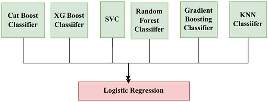
Figure 5. Meta-learner.

Equation 13 shows how the meta-classifier computes the prediction from all the base models. Here, B is the number of base models, y^b is the prediction from the base models, and f-meta is the final estimator, which is a Lasso-regularized logistic regression in this case.

In a meta-learning classifier, prediction is performed through a two-tier process involving multiple base models and a meta-model. The base layer consists of multiple individual models f_b, each trained independently. For every input X, each base model generates its own prediction y^b, as shown in Equation 14. Here, b indexes each base learner, and f_b(X) denotes the prediction made by the b-th model on input X.

$\begin{array}{ll}{y}^b=f_b(X)\forall b\in \left\{1,\dots ,6\right\}& (14)\end{array}$

The predictions from all base learners are then passed to a meta-layer. It learns to combine them optimally. This is performed using logistic regression as the meta-model, with L1 regularization. Equation 15 shows the final prediction being class 1, given all base predictions. Here, y^b is the prediction from the b-th base model, Bw_b is the weight assigned to each base model's output by the meta-model, w₀ is the bias term in the logistic regression, and σ() is the sigmoid activation function used to produce the final probability. To prevent overfitting and increase sparsity, an L1 regularization constraint is placed on the weight vector w, such that ||w||₁ ≤ λ. Here, ||w||₁ represents the L1 norm of the weights, and λ is a hyperparameter controlling the strength of regularization.

$\begin{array}{ll}P\left(y=1|\widehat{y}\right)=\sigma \left(b=1{\displaystyle \sum }B{w}_b{y}^b+w_0\right)& (15)\end{array}$

In the meta-classifier, six base models are employed—namely, CatBoost, XGBoost, SVM, random forest, gradient boosting, and k-nearest neighbors (KNN). CatBoost is a gradient boosting decision tree that is specifically used for categorical data. It is used for effective and precise classification and regression. It encodes the categorical features with target statistics from previous rows (Prokhorenkova et al., 2018). Equation 16 is the encoded value for the categorical feature of the i-th sample. Here, y_j represents the true target values of previous rows, and i-1 ensures that only preceding samples are used, preserving causality and avoiding target leakage. Equation 17 represents the objective function that includes both the loss term and regularization term. Here, n is the total number of samples, L (y_i, F(x_i)) is the loss function, F(x) = $\sum _{t=1}^T{f}_t$ (x) is the model's cumulative prediction over T decision trees, and Ω(f_t) is a regularization function applied to each individual tree f_t.

$\begin{array}{ll}{x}_{cat}^{(i)}=\frac{{\displaystyle {\sum }_{j=1}^{i-1}}{y}_j}{i-1}& (16)\end{array}$

$\begin{array}{ll}L={\displaystyle \sum _{i=1}^{n}L(y_i,F(x_i))}+{\displaystyle \sum _{t=1}^T\Omega }\left(f_t\right)& (17)\end{array}$

XGBoost is another gradient boosting algorithm that minimizes the loss function with a second-order Taylor expansion (Raihan et al., 2023). It is specifically built for high-speed classification and regression tasks, tuning both speed and accuracy. Equation 18 represents the objective function at the t-th iteration. Here, n is the number of training samples, $L(y_i,F^{(t)}(x_i))$ is the loss between the true label and prediction at iteration t, T denotes the number of leaves in the newly added tree, and γ and λ are regularization hyperparameters that penalize complexity. Equation 19 represents the regularization component that encourages simpler trees. Here, γT discourages the number of leaves in the tree, discouraging overly complex models, and $\frac{\lambda }{2}{\parallel w\parallel }^2$ is a regularization term applied to the leaf weights w, controlling their magnitude and enhancing generalization.

$\begin{array}{ll}{L}^{(t)}={\displaystyle \sum _{i=1}^{n}L(y_i,F^{(t)}(x_i))}+\gamma T+\frac{\lambda }{2}\parallel w{\parallel }^2& (18)\end{array}$

$\begin{array}{ll}\Omega (f_t)=\gamma T+\frac{\lambda }{2}{\parallel w\parallel }^2& (19)\end{array}$

SVC identifies a hyperplane that maximizes the margin between two classes. SVC supports linear and non-linear classification with kernel functions. It performs well in high-dimensional spaces and is resistant to overfitting, particularly in situations with a clear margin of separation between classes. Equation 20 represents the dual optimization objective performed by SVC. Here, α_i are the Lagrange multipliers to be improved, and K(x_i, x_j) is the kernel function that maps the data into a higher-dimensional space to make it linearly separable. K(x,z) = e^{−γ||x − z||2} is the radial basis function (RBF) kernel, where γ controls the width of the Gaussian kernel and determines the influence of each training example. This kernelized formulation allows SVC to handle complex, non-linear decision boundaries efficiently while maintaining strong generalization performance.

$\begin{array}{ll}{max}_{\alpha }{\displaystyle \sum _{i=1}^n}{\alpha }_i-\frac{1}{2}{\displaystyle \sum _{i,j}}{\alpha }_i{\alpha }_j{y_{i}y}_{j}K\left(x_i,x_j\right)& (20)\end{array}$

A random forest classifier is a machine learning model that employs many decision trees to classify data, making its predictions based on the majority vote of the individual trees. It is known for its accuracy and stability. It performs this by selecting a random subset of features and training the decision trees on a different subset of the data. The final prediction is made through majority voting (Pal, 2005). Equation 21 represents the prediction rule. Here, ŷ_RF is the final prediction from the random forest, ŷ_treek is the prediction from the k-th decision tree, and mode denotes the majority voting over all trees k = 1…K. Equation 22 represents the sampling correlation formula that is used to find how much the trees in the forest correlate in their predictions. Here, T(x; Z) is the output of a decision tree trained on the data subset Z with random feature sampling θ. Var_z and E_z denote the variance and expectation over the dataset subsets.

$\begin{array}{ll}{\widehat{y}}_{RF}=mode\left({\left\{{\widehat{y}}_{{tree}_k}\right\}}_{k=1}^K\right)& (21)\end{array}$

$\begin{array}{ll}\rho \left(x\right)=\frac{Va{r}_z[E_{\Theta }[T(x;Z)]]}{Va{r}_z[E_{\Theta }[T(x;Z)]]+E_z[Va{r}_{\Theta }[T(x;Z)]]}& (22)\end{array}$

The gradient boosting classifier is an ensemble learning algorithm that constructs multiple decision trees sequentially, where each new tree corrects the errors of the previous ones. It reduces the loss function by optimizing residual errors using gradient descent. Gradient boosting combines weak learners to create a strong predictive model. Equation 23 denotes the prediction function at iteration m. Here, F_m(x) is the updated model after the m-th iteration, h_m(x) is the weak learner added at stage mmm, which fits the negative gradient of the loss function, and γ_m is the step size or weight for the m-th learner.

$\begin{array}{ll}{F}_m(x)=F_{m-1}(x)+{\gamma }_m{h}_m(x)& (23)\end{array}$

The KNN classifier is a machine learning algorithm that is non-parametric. It classifies an instance based on the majority class among its k closest neighbors in the feature space. The algorithm depends on distance metrics to compute similarity between points (Cunningham and Delany, 2021). Equation 25 represents the prediction rule of KNN. Here, N_k(x) denotes the set of KNN of instance x, and y_j represents the label of the neighbor x_j. Equation 25 provides the formula to calculate the distance between the points. Here, x_ix_j are two points in a p-dimensional space.

$\begin{array}{ll}{\widehat{y}}_{KNN}=mode{\displaystyle \left(\left\{\{y_j|x_j\in N_k(x)\right\}\right)}& (24)\end{array}$

$\begin{array}{ll}d(x_i,x_j)=\sqrt{{\displaystyle \sum _{k=1}^p}{(x_{ik}-x_{jk})}^2}& (25)\end{array}$

A meta-learner using logistic regression with Lasso regularization is an advanced ensemble learning technique, where logistic regression serves as the final classifier in the meta-learning model. Lasso (L1) regularization is applied to enforce sparsity by shrinking less important coefficients to zero, effectively performing feature selection. Equation 26 represents the objective function. Here, p_i = σ(w₀ + w₁x₁ + ... + w_px_p), Lasso penalty (||w||₁||w||₁) encourages sparsity, ŷ_i is the prediction from base learners, σ is the sigmoid function, w is the weight vector, ||w||₁ is the L1-norm of the weights, and λ is the regularization strength.

$\begin{array}{ll}{\min }_w=-{\displaystyle \sum _{i=1}^n{y}_i\log \sigma (w^T{\widehat{y}}_i)+(1-y_i)\log (1-\sigma (w^T{\widehat{y}}_i))}+\lambda {\left|\left|w\right|\right|}_1& (26)\end{array}$

2.2.5 Explainable AI and digital twins

2.2.5.1 Grad-CAM

Grad-CAM produces class-discriminative visualizations by combining gradients and convolutional feature maps. For a target class c, the localization heatmap $L_{Grad-CAM}^c$ is computed, as seen in Equation 28.

$\begin{array}{ll}{\propto }_k^c=\frac{1}{Z}{\displaystyle \sum _i}{\displaystyle \sum _j}\frac{\partial y^c}{\partial A_{ij}^k}& (27)\end{array}$

$\begin{array}{ll}{L}_{Grad-CAM}^c=ReLU\left({\displaystyle \sum _k}{\propto }_k^c{A}^k\right)& (28)\end{array}$

Here, A^k are the activations from the final convolutional layer, ${\propto }_k^c$ are the gradient weights, and Z normalizes the spatial dimensions.

2.2.5.2 Saliency map

Saliency maps detect influential pixels in input images by calculating gradients of class scores with respect to input pixels. For a class c, the saliency map S is derived using Equation 29, where y^c is the class score and x_ij are the input pixels. Such maps highlight regions that most strongly influence predictions, regardless of the model's architecture.

$\begin{array}{ll}{S}_{ij}={\displaystyle \underset{k}{max}}{\displaystyle \left|\frac{\partial y^c}{\partial x_{ij}}\right|}& (29)\end{array}$

2.2.5.3 Digital twins

Digital twin is envisioned as an imaginary twin of the diagnostic model that reflects its behavior and decision path through real-time input–output mapping. Leveraging Grad-CAM and saliency map visualizations, the digital twin allows clinicians and researchers to understand how the system detects suspicious areas in dermoscopic images. Each component of the pipeline—the early activation block, deep feature extraction, feature refinement based on t-SNE, the meta-learning classifier, and the interpretability modules, such as Grad-CAM—is a layer of the digital twin. This combination allows the system to reflect in real time and adapt much like a human expert would. This digital representation allows for real-time simulation and verification of the diagnostic process, providing insights into model behavior under different input conditions. It not only adds transparency but also serves as a feedback loop for model optimization by examining performance across different patient populations and image modalities. Embedding this notion in the visualization module guarantees not just correct predictions but also traceability and explainability, fostering trust in clinical environments for AI-supported diagnosis. The conclusion must be an explicit improvement: the digital twin provides interpretability, a real-time personal simulation, and transparency in the outcomes, allowing our model to evolve from a black-box classifier to a self-aware diagnostic assistant that respects the tenets of digital twinning in healthcare AI.

3 Results

The sample distribution of the training and test sets is shown in Figure 6, highlighting any possible class imbalance. The dataset is split in a ratio of 80:20, with 360 images in the test set and 1,440 in the training set. Figure 7 shows the count of images in each class. Having a balanced dataset is important for fair model performance since models trained on imbalanced datasets may learn to favor the majority class.

Figure 6

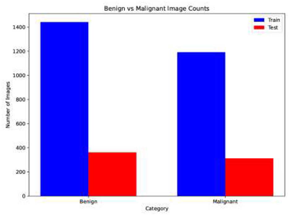
Figure 6. Count of images of each class after train-test split.

Figure 7

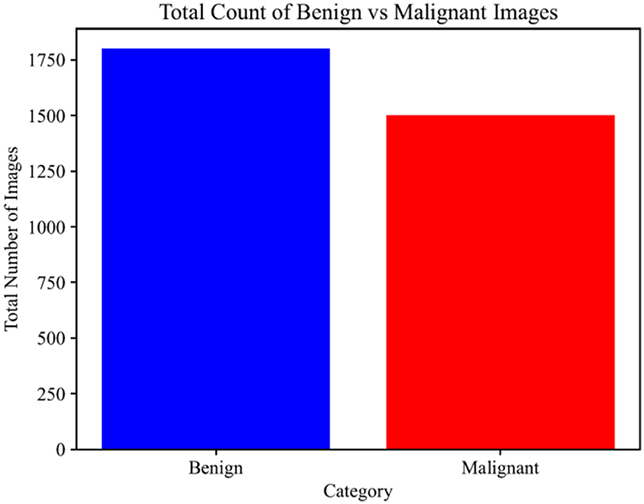
Figure 7. Total count of images of each class.

The pre-trained model was trained on the ISIC dataset, which contains two classes: benign and malignant, as seen in Figure 7. The model obtained a test accuracy of 90%, indicating that it is very effective in discriminating between the two classes. The plot of training and validation accuracy shown in Figure 12 illustrates how accuracy varies as the number of epochs increases. To obtain better feature representations learned by the model, we employed t-SNE, a non-linear dimensionality reduction technique. Figures 8–11 visualize how different layers separate the benign and malignant classes. The layer that was well clustered was selected for feature extraction, as it demonstrated high discriminative power, as shown in Figure 12.

Figure 8

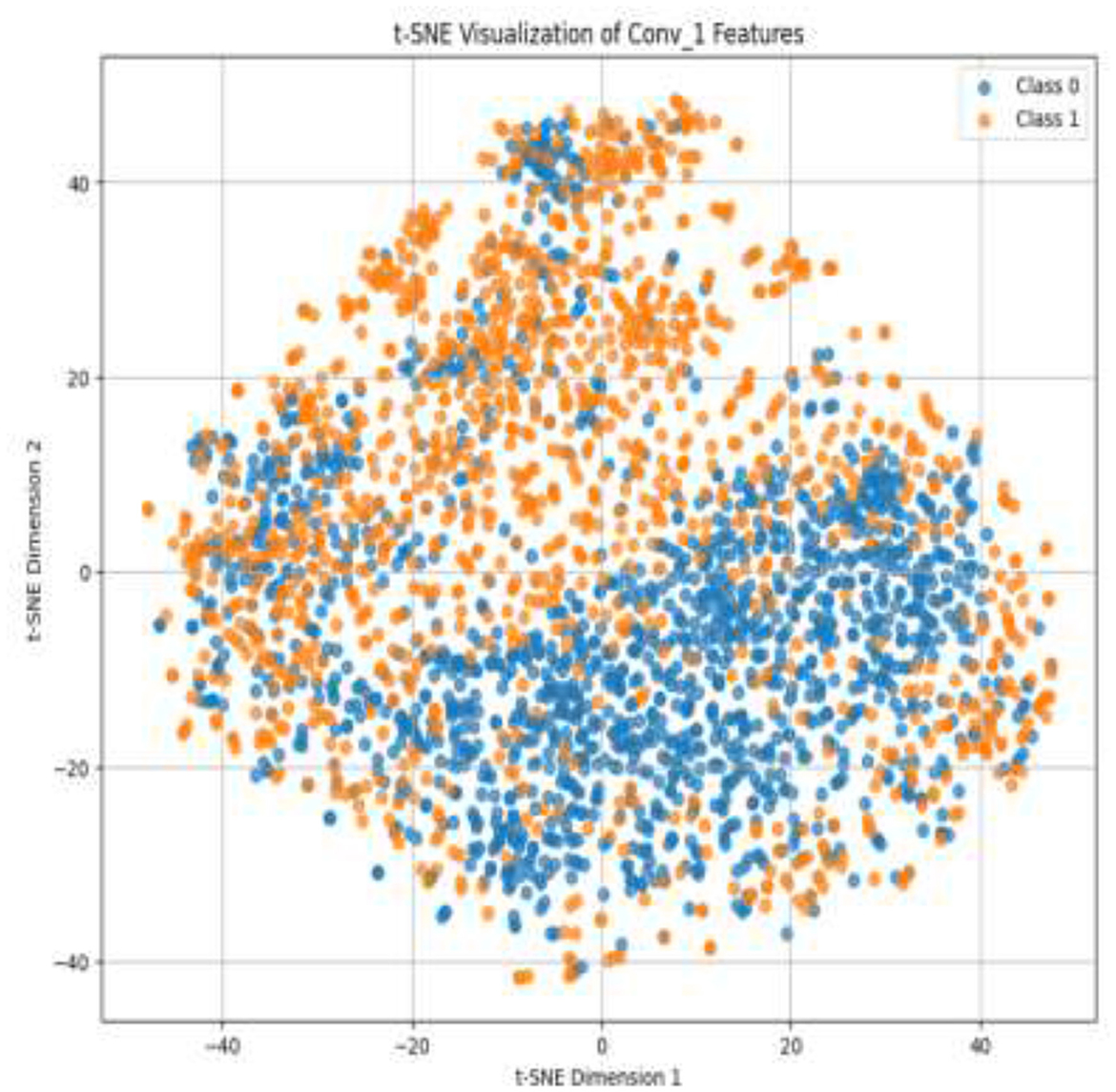
Figure 8. t-SNE visualization of the Conv_1.

Figure 9

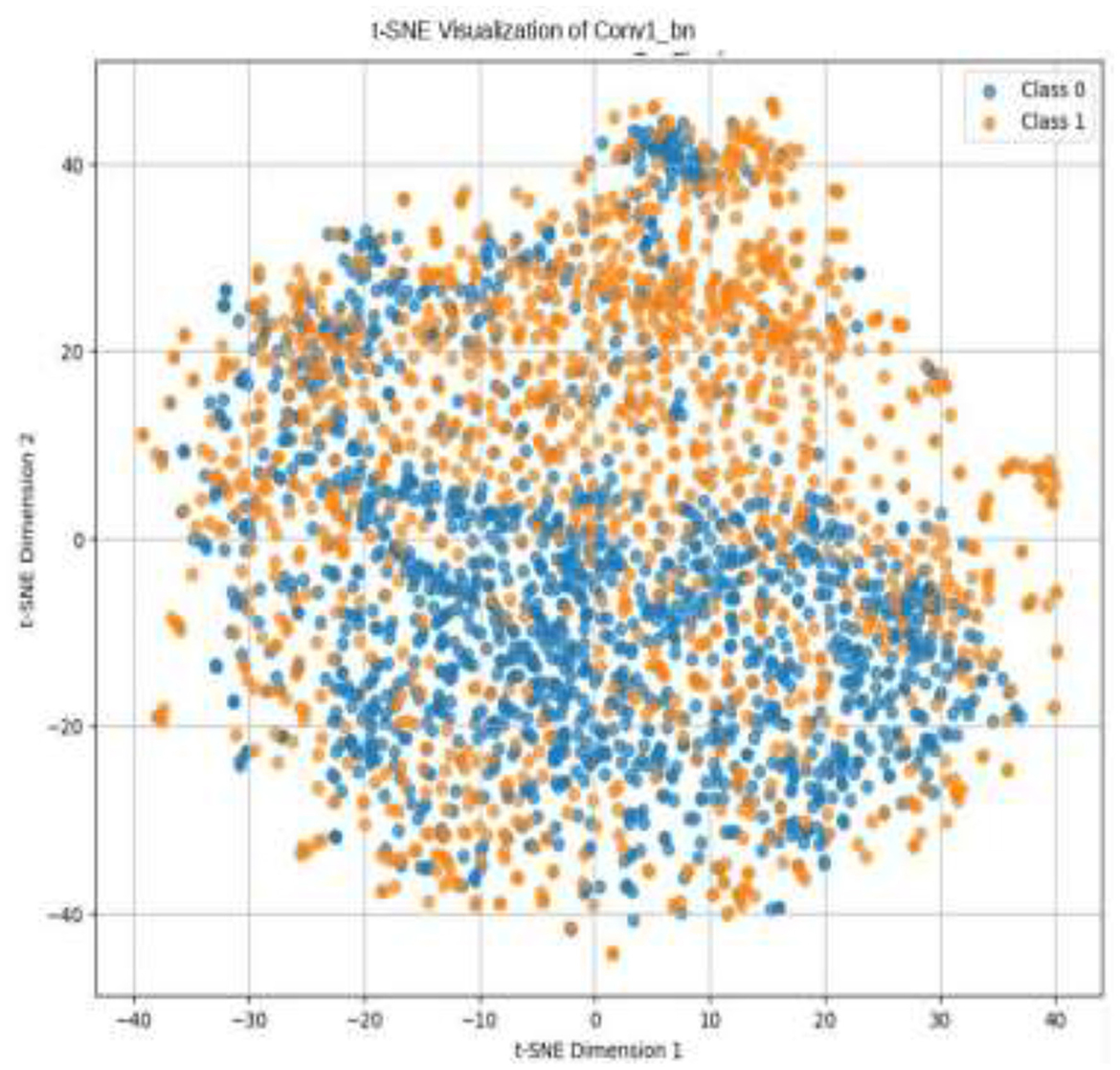
Figure 9. t-SNE visualization of the Conv1_bn.

Figure 10

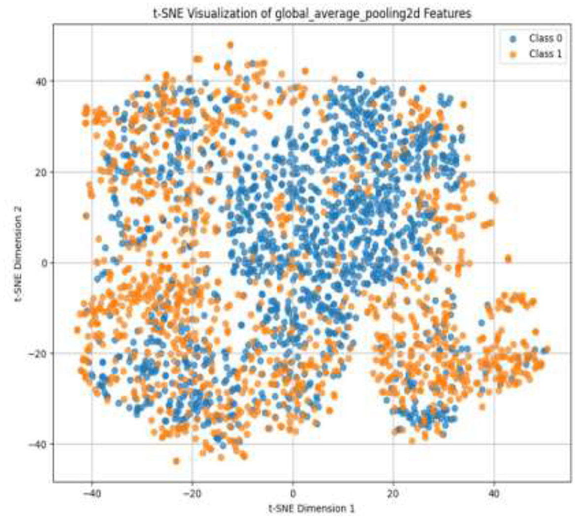
Figure 10. t-SNE visualization of the global_average_pooling2d.

Figure 11

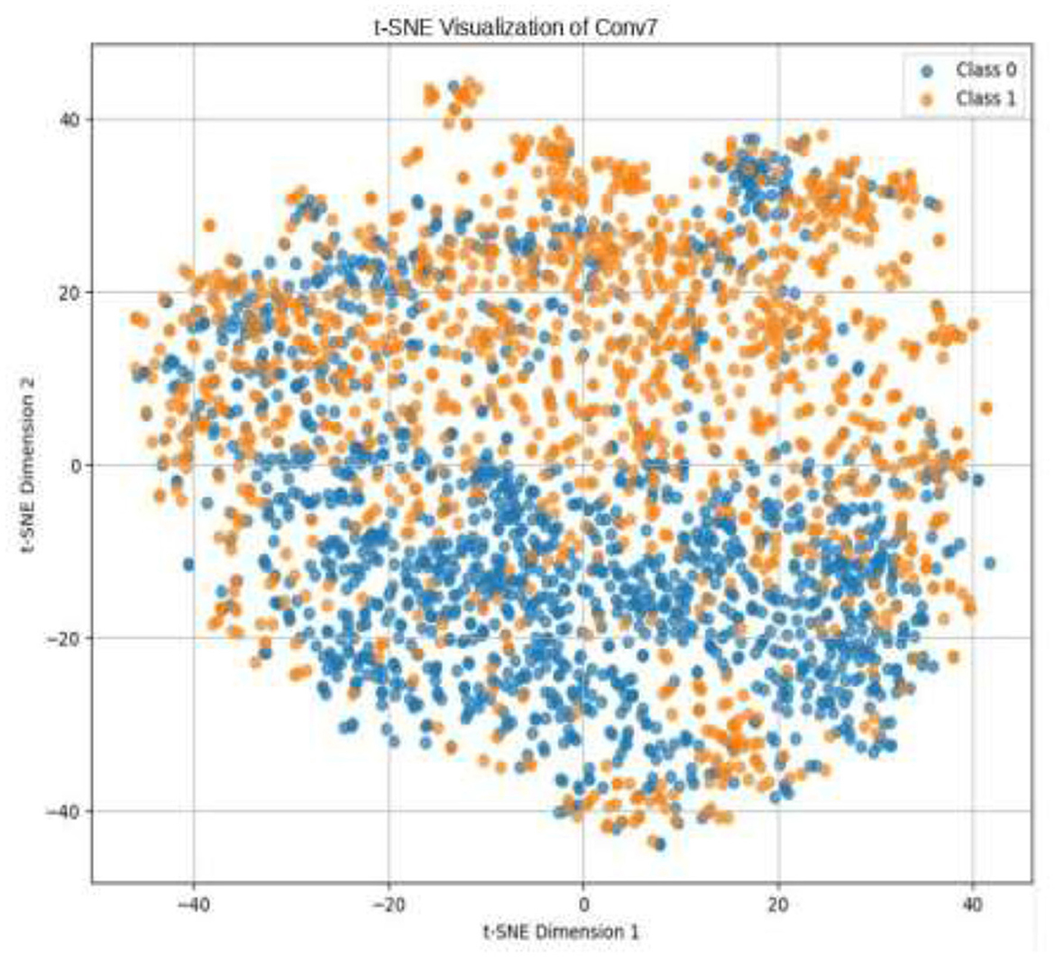
Figure 11. t-SNE visualization of the Conv7.

Figure 12

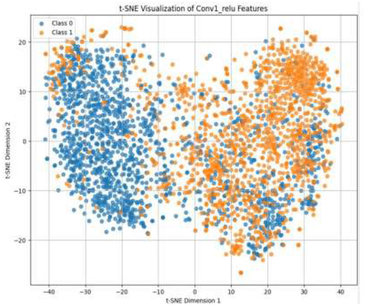
Figure 12. t-SNE visualization of the Conv1_relu.

Following feature extraction from the most learnable layer, the extracted features were used to train a meta-learning classifier. The t-SNE visualization of the Conv1_relu layer in Figure 12 shows a moderate level of feature separation between the benign and malignant cases. Figure 13 illustrates the confusion matrices and ROC curves for each individual classifier, and Figure 14 shows the combined performance achieved using the proposed meta-learning classifier. Among all, the proposed classifier achieved the highest accuracy, clearly outperforming the individual models and demonstrating the effectiveness of the ensemble approach. Figure 15 shows the Line graph showing training and validation accuracy overtwenty epochs. In addition, the t-SNE visualization in Figure 16 provides a more optimal clustering of the two classes. From these visualizations, we can see the improved classification performance of the meta-learning classifier compared to the pre-trained model alone. Figure 17 shows the meta visualization of skin cancer analysis for the benign class. Figure 18 shows the Grad-CAM visualization and saliency map of malignant.

Figure 13

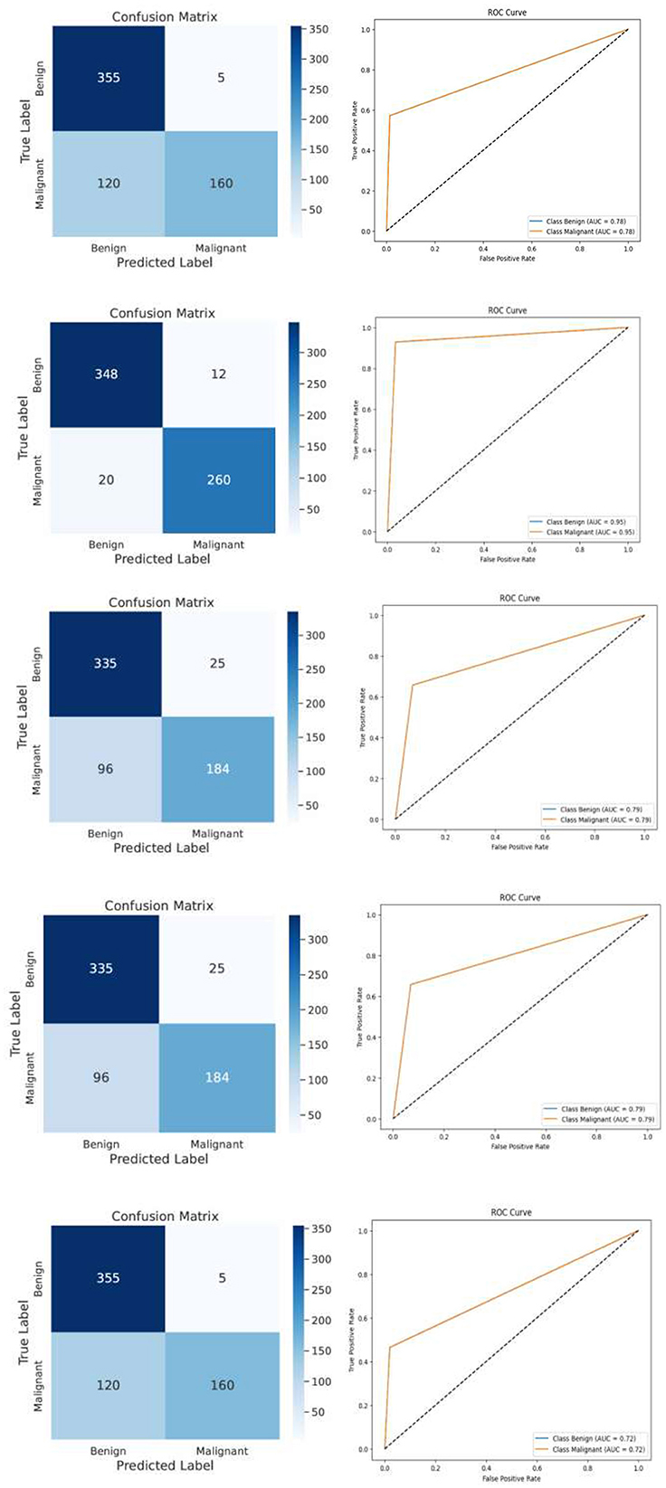
Figure 13. Classification report and ROC curve of the base models.

Figure 14

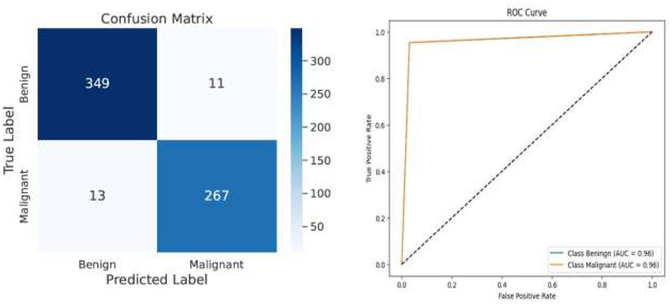
Figure 14. Classification report and ROC curve of the meta-learning classifier.

Figure 15

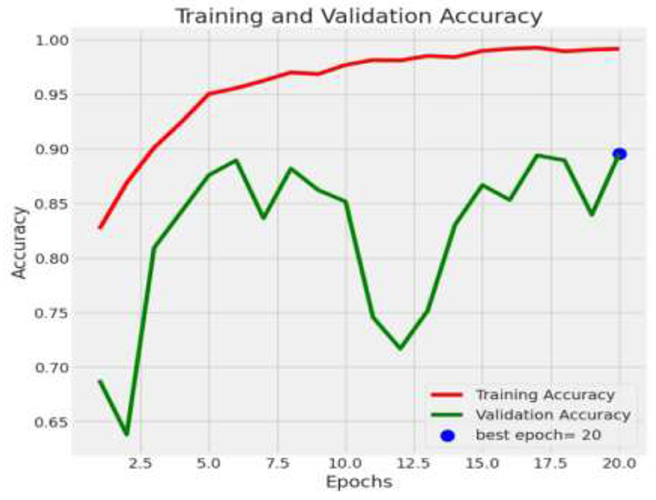
Figure 15. Plot of training and validation accuracy.

Figure 16

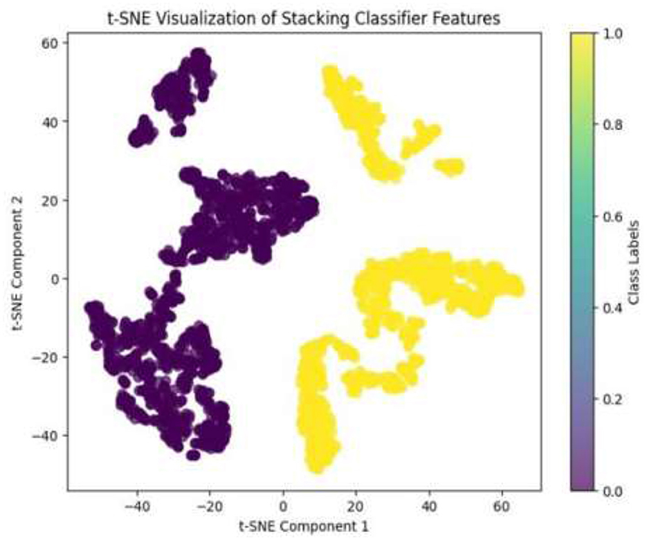
Figure 16. t-SNE visualization of meta-learning classifier.

Figure 17

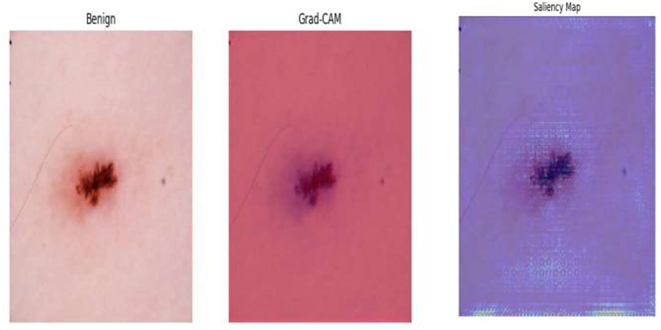
Figure 17. Grad-CAM visualization and saliency map of benign.

Figure 18

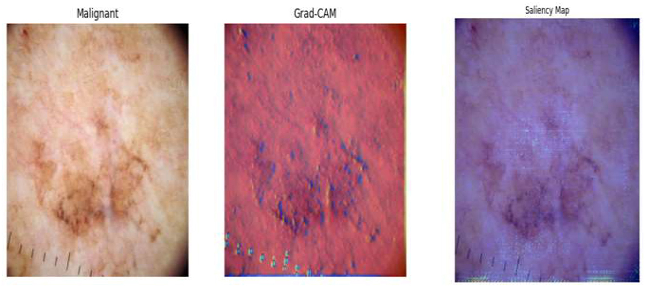
Figure 18. Grad-CAM visualization and saliency map of malignant.

These findings shown in Table 2 suggest that deep learning models work extremely well for skin cancer detection if trained with the ISIC dataset. The utilization of t-SNE visualization to identify the most informative features, followed by the application of a meta-learning classifier, further improved the performance. The fact that this process worked so well highlights the importance of feature selection in medical image classification using deep learning.

Table 2

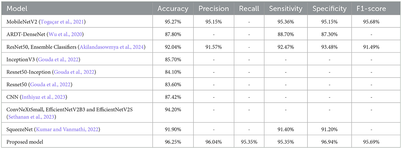
Table 2. Comparison with the proposed model.

4 Discussion

Skin cancer is a significant global health problem, and thus there is a need for effective and accurate diagnosis techniques. The suggested model integrates deep feature extraction with a meta-learning classifier to achieve enhanced classification performance. The model applies t-SNE visualization to identify the most informative learnable layers to reduce feature selection and computational complexity. The proposed methodology was tested with respect to standard deep learning-based models and was found to perform more efficiently without losing accuracy. The model displayed 96.25% accuracy, which made it a trustworthy tool for skin cancer classification. Such AI-based testing can provide an attractive alternative to manual diagnosis methods for dermatologists, providing early and accurate detection capabilities. A digital twin platform is integrated to virtually replicate the diagnostic workflow for continuous monitoring, optimization, and model validation within a safe environment. In addition, explainable AI methods are used to provide transparency by identifying the salient image regions that are driving the model's predictions. Future development may involve incorporating a wider range of dermatological data sources and implementing dynamic validation in live clinical settings to further enhance performance and accessibility. In our future work, we hope to broaden the boundaries of the proposed framework by integrating heterogeneous dermatology data sources, including clinical images, patient metadata, and histopathological data, to improve model generalizability and robustness. We will also aim to conduct real-time validations in live clinical environments to understand practicality, adaptability, and end-user's views and feedback on the real-world application of the diagnostic tool. Overall, a deeper investigation into automated feature selection, mobile-embedded device integration, and potential alternatives including continual learning may help develop the scalability and clinical viability of the system.

Data availability statement

The original contributions presented in the study are included in the article/supplementary material, further inquiries can be directed to the corresponding author.

Author contributions

PS: Writing – original draft, Methodology. GS: Writing – original draft, Software. SV: Writing – original draft, Validation. YK: Writing – original draft, Visualization. SS: Writing – review & editing, Funding acquisition, Conceptualization.

Funding

The author(s) declare that financial support was received for the research and/or publication of this article. This work was supported by the National Research Foundation of Korea (NRF) grant funded by the Korea government (MSIT) (No. RS-2023-00218176) and the MSIT (Ministry of Science and ICT), Korea, under the Convergence security core talent training business support program (IITP-2025-RS-2023-00266605) supervised by the IITP (Institute for Information & Communications Technology Planning & Evaluation).

Conflict of interest

The authors declare that the research was conducted in the absence of any commercial or financial relationships that could be construed as a potential conflict of interest.

Generative AI statement

The author(s) declare that no Gen AI was used in the creation of this manuscript.

Publisher's note

All claims expressed in this article are solely those of the authors and do not necessarily represent those of their affiliated organizations, or those of the publisher, the editors and the reviewers. Any product that may be evaluated in this article, or claim that may be made by its manufacturer, is not guaranteed or endorsed by the publisher.

References

Akilandasowmya, G., Nirmaladevi, G., Suganthi, S. U., and Aishwariya, A. (2024). Skin cancer diagnosis: leveraging deep hidden features and ensemble classifiers for early detection and classification. Biomed. Signal Process Control 88:105306. doi: 10.1016/j.bspc.2023.105306

Crossref Full Text | Google Scholar

Akter, M., Khatun, R., Talukder, M. A., Islam, M. M., Uddin, M. A., Ahamed, M. K. U., et al. (2025). An integrated deep learning model for skin cancer detection using hybrid feature fusion technique. Biomed. Mater. Devices 3, 1–15. doi: 10.1007/s44174-024-00264-3

Crossref Full Text | Google Scholar

Alharbi, H., Sampedro, G. A., Juanatas, R. A., and Lim, S. J. (2024). Enhanced skin cancer diagnosis: a deep feature extraction-based framework for the multi-classification of skin cancer utilizing dermoscopy images. Front. Med. 11:1495576. doi: 10.3389/fmed.2024.1495576

PubMed Abstract | Crossref Full Text | Google Scholar

Amin, J., Sharif, A., Gul, N., Anjum, M. A., Nisar, M. W., Azam, F., et al. (2020). Integrated design of deep features fusion for localization and classification of skin cancer. Pattern Recognit. Lett. 131, 63–70. doi: 10.1016/j.patrec.2019.11.042

Crossref Full Text | Google Scholar

Brancaccio, G., Balato, A., Malvehy, J., Puig, S., Argenziano, G., Kittler, H., et al. (2024). Artificial intelligence in skin cancer diagnosis: a reality check. J. Invest. Dermatol. 144, 492–499. doi: 10.1016/j.jid.2023.10.004

PubMed Abstract | Crossref Full Text | Google Scholar

Claret, S. A., Dharmian, J. P., and Manokar, A. M. (2024). Artificial intelligence-driven enhanced skin cancer diagnosis: leveraging convolutional neural networks with discrete wavelet transformation. Egypt J. Med. Hum. Genet. 25:50. doi: 10.1186/s43042-024-00522-5

Crossref Full Text | Google Scholar

Cunningham, P., and Delany, S.J. (2021). K-nearest neighbour classifiers-a tutorial. ACM Comput. Surv. 54, 1–25. doi: 10.1145/3459665

Crossref Full Text | Google Scholar

Ekmekyapar, T., and Taşci, B. (2023). Exemplar MobileNetV2-based artificial intelligence for robust and accurate diagnosis of multiple sclerosis. Diagnostics 13:3030. doi: 10.3390/diagnostics13193030

PubMed Abstract | Crossref Full Text | Google Scholar

Georgiou, T., Liu, Y., Chen, W., and Lew, M. (2020). A survey of traditional and deep learning-based feature descriptors for high dimensional data in computer vision. Int. J. Multimed. Inf. Retr. 9, 135–170. doi: 10.1007/s13735-019-00183-w

Crossref Full Text | Google Scholar

Gouda, W., Sama, N. U., Al-Waakid, G., Humayun, M., and Jhanjhi, N. Z. (2022). Detection of skin cancer based on skin lesion images using deep learning. Healthcare 10:1183. doi: 10.3390/healthcare10071183

PubMed Abstract | Crossref Full Text | Google Scholar

Himel, G. M. S., Islam, M. M., Al-Aff, K. A., Karim, S. I., and Sikder, M. K. U. (2024). Skin cancer segmentation and classification using vision transformer for automatic analysis in dermatoscopy-based noninvasive digital system. Int. J. Biomed. Imaging 2024:3022192. doi: 10.1155/2024/3022192

PubMed Abstract | Crossref Full Text | Google Scholar

Inthiyaz, S., Altahan, B. R., Ahammad, S. H., Rajesh, V., Kalangi, R. R., Smirani, L. K., et al. (2023). Skin disease detection using deep learning. Adv. Eng. Softw. 175:103361. doi: 10.1016/j.advengsoft.2022.103361

Crossref Full Text | Google Scholar

Itoo, N. N., and Garg, V. K. (2022). “Heart disease prediction using a stacked ensemble of supervised machine learning classifiers,” in Proceedings of the 2022 International Mobile and Embedded Technology Conference (MECON) (Noida: IEEE), 599–604. doi: 10.1109/MECON53876.2022.9751883

Crossref Full Text | Google Scholar

Kanchana, K., Kavitha, S., Anoop, K. J., and Chinthamani, B. (2024). Enhancing skin cancer classification using efficient net B0-B7 through convolutional neural networks and transfer learning with patient-specific data. Asian Pac. J. Cancer Prev. 25:1795. doi: 10.31557/APJCP.2024.25.5.1795

PubMed Abstract | Crossref Full Text | Google Scholar

Kumar, K. A., and Vanmathi, C. (2022). Optimization driven model and segmentation network for skin cancer detection. Comput. Electr. Eng. 103:108359. doi: 10.1016/j.compeleceng.2022.108359

Crossref Full Text | Google Scholar

Mahmud, F., Mahfiz, M. M., Kabir, M. Z. I., and Abdullah, Y. (2023). “An interpretable deep learning approach for skin cancer categorization,” in 2023 26th International Conference on Computer and Information Technology (IC-CIT) (Cox's Bazar: IEEE), 1–6. doi: 10.1109/ICCIT60459.2023.10508527

Crossref Full Text | Google Scholar

Melarkode, N., Srinivasan, K., Qaisar, S. M., and Plawiak, P. (2023). AI-powered diagnosis of skin cancer: a contemporary review, open challenges and future research directions. Cancers 15:1183. doi: 10.3390/cancers15041183

PubMed Abstract | Crossref Full Text | Google Scholar

Naqvi, M., Gilani, S. Q., Syed, T., Marques, O., and Kim, H.C. (2023). Skin cancer detection using deep learning-a review. Diagnostics 13:1911. doi: 10.3390/diagnostics13111911

PubMed Abstract | Crossref Full Text | Google Scholar

Pal, M. (2005). Random Forest classifier for remote sensing classification. Int. J. Remote Sens. 26, 217–222. doi: 10.1080/01431160412331269698

Crossref Full Text | Google Scholar

Prokhorenkova, L., Gusev, G., Vorobev, A., Dorogush, A. V., and Gulin, A. (2018). “CatBoost: unbiased boosting with categorical features,” in Advances in Neural Information Processing Systems (NeurIPS) (Cambridge, MA: The MIT Press).

Google Scholar

Ragab, M., Alshehri, S., Azim, G. A., Aldawsari, H. M., Noor, A., Alyami, J., et al. (2022). COVID-19 identification system using transfer learning technique with MobileNetV2 and chest X-ray images. Front. Public Health 10:819156. doi: 10.3389/fpubh.2022.819156

PubMed Abstract | Crossref Full Text | Google Scholar

Raihan, M. J., Khan, M. A. M., Kee, S. H., and Nahid, A.A. (2023). Detection of the chronic kidney disease using XGBoost classifier and explaining the influence of the attributes on the model using SHAP. Sci. Rep. 13:6263. doi: 10.1038/s41598-023-33525-0

PubMed Abstract | Crossref Full Text | Google Scholar

Salinas, M. P., Sepúlveda, J., Hidalgo, L., Peirano, D., Morel, M., Uribe, P., et al. (2024). A systematic review and meta-analysis of artificial intelligence versus clinicians for skin cancer diagnosis. NPJ Digit. Med. 7:125. doi: 10.1038/s41746-024-01103-x

PubMed Abstract | Crossref Full Text | Google Scholar

Sandler, M., Howard, A., Zhu, M., Zhmoginov, A., and Chen, L. C. (2018). “Mobilenetv2: inverted residuals and linear bottlenecks,” in Proceedings of the IEEE Conference on Computer Vision and Pattern Recognition (CVPR) (Salt Lake City, UT: IEEE), 4510–4523. doi: 10.1109/CVPR.2018.00474

PubMed Abstract | Crossref Full Text | Google Scholar

Sawal, S., and Kathait, S.S. (2023). MobileNetV2: transfer learning for elephant detection. Int. J. Comput. Appl. 975, 59–65. doi: 10.5120/ijca2025924403

PubMed Abstract | Crossref Full Text | Google Scholar

Sethanan, K., Pitakaso, R., Srichok, T., Khonjun, S., Thannipat, P., Wanram, S., et al. (2023). Double AMIS-ensemble deep learning for skin cancer classification. Expert Syst. Appl. 234:121047. doi: 10.1016/j.eswa.2023.121047

Crossref Full Text | Google Scholar

Surya, A., Shah, A., Kabore, J., and Sasikumar, S. (2023). Enhanced breast cancer tumor classification using MobileNetV2: a detailed exploration on image intensity, error mitigation, and streamlit-driven real-time deployment. arXiv. doi: 10.48550/arXiv.2312.03020

Crossref Full Text | Google Scholar

Tai, C. E. A., Janes, E., Czarnecki, C., and Wong, A. (2024). Double-condensing attention condenser: leveraging attention in deep learning to detect skin cancer from skin lesion images. Sensors 24:7231. doi: 10.3390/s24227231

PubMed Abstract | Crossref Full Text | Google Scholar

Thompson, N. C., Greenewald, K., Lee, K., and Manso, G. F. (2020). The computational limits of deep learning. arXiv. doi: 10.48550/arXiv.2007.05558

Crossref Full Text | Google Scholar

Tika Adilah, M., and Kristiyanti, D. A. (2023). Implementation of transfer learning MobileNetV2 architecture for identification of potato leaf disease. J. Theor. Appl. Inf. Technol. 101, 6273–6285.

Google Scholar

Togaçar, M., Cömert, Z., and Ergen, B. (2021). Intelligent skin cancer detection applyingautoencoder, MobileNetV2 and spiking neural networks. Chaos Solitons Fractals 144:110714. doi: 10.1016/j.chaos.2021.110714

Crossref Full Text | Google Scholar

Van der Maaten, L., and Hinton, G. (2008). Visualizing data using t-SNE. J. Mach. Learn Res. 9, 2579–2605.

Google Scholar

Villa-Pulgarin, J. P., Ruales-Torres, A. A., Arias-Garzon, D., Bravo-Ortiz, M. A., Arteaga-Arteaga, H. B., Mora-Rubio, A., et al. (2022). Optimized convolutional neural network models for skin lesion classification. Comput. Mater. Continua. 70, 2131–2148. doi: 10.32604/cmc.2022.019529

Crossref Full Text | Google Scholar

Wang, M., Gao, X., and Zhang, L. (2025). Recent global patterns in skin cancer incidence, mortality, and prevalence. Chin. Med. J. 138, 185–192. doi: 10.1097/CM9.0000000000003416

PubMed Abstract | Crossref Full Text | Google Scholar

Wei, M. L., Tada, M., So, A., and Torres, R. (2024). Artificial intelligence and skin cancer. Front. Med. 11:1331895. doi: 10.3389/fmed.2024.1331895

PubMed Abstract | Crossref Full Text | Google Scholar

Wu, J., Hu, W., Wen, Y., Tu, W., and Liu, X. (2020). Skin lesion classification using densely connected convolutional networks with attention residual learning. Sensors 20:7080. doi: 10.3390/s20247080

PubMed Abstract | Crossref Full Text | Google Scholar

Xu, L., and Mohammadi, M. (2024). Brain tumor diagnosis from MRI based on Mobilenetv2 optimized by contracted fox optimization algorithm. Heliyon 10:e23866. doi: 10.1016/j.heliyon.2023.e23866

PubMed Abstract | Crossref Full Text | Google Scholar

Yuan, W., Du, Z., and Han, S. (2024). Semi-supervised skin cancer diagnosis based on self-feedback threshold focal learning. Discov. Oncol. 15:180. doi: 10.1007/s12672-024-01043-8

PubMed Abstract | Crossref Full Text | Google Scholar

Zhang, N., Cai, Y. X., Wang, Y. Y., Tian, Y. T., Wang, X. L., and Badami, B. (2020). Skin cancer diagnosis based on optimized convolutional neural network. Artif. Intell. Med. 102:101756. doi: 10.1016/j.artmed.2019.101756

PubMed Abstract | Crossref Full Text | Google Scholar

Zhu, Q., Zhuang, H., Zhao, M., Xu, S., and Meng, R. (2024). A study on expression recognition based on improved mobilenetV2 network. Sci. Rep. 14:8121. doi: 10.1038/s41598-024-58736-x

PubMed Abstract | Crossref Full Text | Google Scholar