 Marianthi Markatou
 Elisavet M. Sofikitou
- Department of Biostatistics, SPHHP, University at Buffalo, Buffalo, NY, United States
Over the past years, distances and divergences have been extensively used not only in the statistical literature or in probability and information theory, but also in other scientific areas such as engineering, machine learning, biomedical sciences, as well as ecology. Statistical distances, viewed either as building blocks of evidence generation or as evidence generation vehicles in themselves, provide a natural way to create a global framework for inference in parametric and semiparametric models. More precisely, quadratic distance measures play an important role in goodness-of-fit tests, estimation, prediction or model selection. Provided that specific properties are fulfilled, alternative statistical distances (or divergences) can effectively be used to construct evidence functions. In the present article, we discuss an intrinsic approach to the notion of evidence and present a brief literature review related to its interpretation. We examine several statistical distances, both quadratic and non-quadratic, and their properties in relation to important aspects of evidence generation. We provide an extensive description of their role in model identification and model assessment. Further, we introduce an explanatory plot that is based on quadratic distances to visualize the strength of evidence provided by the ratio of standardized quadratic distances and exemplify its use. In this setting, emphasis is placed on determining the sense in which we can provide meaningful interpretations of the distances as measures of statistical loss. We conclude by summarizing the main contributions of this work.
1. Introduction
What is evidence? The Oxford dictionary defines evidence as “the available body of facts or information indicating whether a belief or proposition is true or valid.” The fundamental knowledge of a science or an art, which at the same time embeds basic philosophical principles, can also be characterized as evidence.
In the scientific world the concept of evidence is crucial as it accumulates all the pieces/sources of information one has at hand and can assess in a variety of ways to judge whether something is true or not. The term statistical evidence (Royall, 2004) refers to observations interpreted under a probability model. To reject or support a hypothesis we use data obtained from the phenomena that occur in the natural world or we perform experiments and combine/match with some background information, resources and scientific tools such as theories, tests and models.
How do we measure the strength of evidence? In statistics, different strategies have been suggested to measure the strength of evidence. Fisher's method (Fisher, 1935) uses extreme value probabilities known as p-values from several independent tests which consider the same null hypothesis. Fisher's p-value tests may provide a measure of evidence (Cox, 1977); however, only a single hypothesis is taken into consideration and no reference to any alternative hypothesis is provided. On the contrary, in Neyman-Pearson tests the decision rule is based on two competing hypotheses, the null hypothesis H0 and the alternative hypothesis H1. This approach divides all the possible outcomes of the sample space into two distinct regions, the acceptance and the rejection region. The specific data values that lead to the rejection of H0 form the rejection region. The aim is to define the best significant level a, that is the probability of rejecting the null hypothesis when in fact it is true. According to Lewin-Koh et al. (2004), Neyman-Pearson tests may not provide an appropriate measure of evidence, in the sense that a decision should be made between two hypotheses of which one is accepted and the other is rejected. As a result, minor data changes could alter the final decision making (Taper and Lele, 2004).
Under the Bayesian framework, the decision is made based on some prior probabilities which try to quantify the scientist's belief about the competing hypotheses. The stronger the scientist's belief is that a hypothesis is true, the higher probability this hypothesis is given. The use of Bayesian tests to measure the strength of evidence has raised questions as the priors' choice may not be objective (Lewin-Koh et al., 2004). Bayesianism as well as likelihoodism are both based on the same principle, the law of likelihood (Sober, 2008). Likelihood and, by extension, likelihood ratio are basic statistical tools used for the quantification of the strength of evidence. For instance, consider the case where there are two hypotheses H0 : τ = mθ0 vs. H1 : τ = mθ1; then, the likelihood ratio is defined by L(θ0; x)/L(θ1; x). The likelihood ratio of H0 vs. H1 measures the strength of evidence for the first hypothesis H0 vs. the second hypothesis H1. A likelihood ratio takes values that are greater than or equal to zero; a value of one indicates that the evidence does not support one hypothesis over the other. On the other hand, a value of the likelihood ratio substantially greater than 1, indicates support of H1 vs. H0.
The evidential paradigm uses likelihood ratios as measures of statistical evidence for or against hypotheses of interest. Royall (1997, 2000, 2004) suggests that the use of likelihood ratio to quantify strength of evidence of one model over another. Although likelihood ratio is a useful measure of strength of evidence, it has some practical limitations. More precisely, it is sensitive to outliers and it requires the specification of a complete statistical model (Lele, 2004).
However, all the basic theories of inference and evidence described above have disadvantages. To overcome their drawbacks, these techniques have been extended to address the problem of multiple comparisons and composite hypotheses testing, as well as to deal with situations where nuisance parameters are present. In particular, Royall (2000) suggests the use of profile monitoring for evidential inference purposes when one has to cope with nuisance parameters and composite hypotheses. A further, though quite challenging, generalization would be the case of unequal nuisance parameter number between the compared models (Taper and Lele, 2004). Moreover, the idea of evidence and its measurement has been extended to model adequacy and selection problems.
Fundamental to scientific work is the use of models. In analyzing and interpreting data, the use of models, explicit or implicit, is unavoidable. Models are used to summarize statistical properties of data, to identify parameters, and to evaluate different policies. Where do models come from? The literature provides very little help on answering the question of model formulation, yet this is arguably the most difficult aspect of model building. Cox (1990) and Lehmann (1990) discuss this question and offer various classifications of statistical models. Following Cox (1990), we define a statistical model as:
(1) A specification of a joint probability distribution of a single random variable or a vector of random variables,
(2) A definition of a vector of parameters of interest, ideally such that each component of the vector has a subject-matter interpretation as representing some understandable stable property of the system under study, and
(3) At least an indication of or a link with the process that could have generated the data.
In this paper, we are not concerned with the origins of models. We take as given that a class of models is under consideration and we are concerned with methods of obtaining evidence characterizing the quality of an aspect of model assessment, that is the adequacy of a model in answering questions of interest and/or our ability to perform model selection. Measuring model adequacy centers on measuring the model misspecification cost. Lindsay (2004) discusses a distance-based framework for assessing model adequacy, a fundamental tenet of which is that one is able to carry out a model-based scientific inquiry without assuming that the model is true and without assuming that “truth” belongs in the model class under investigation. However, we make the assumption that the “truth” exists and it is knowable given the presence of data. The evidence for the adequacy of the model is measured via the concept of a statistical distance.
We discuss therefore statistical distances as evidence functions in the context of model assessment. We show that statistical distances that can be interpreted as loss functions can be used as evidence functions. We discuss in some detail a specific class of statistical distances, called quadratic distances, and illustrate their use in applications. For ease of presentation, we only use simple hypotheses, however these measures can handle both simple and composite hypotheses. Methods based on distances compare models by estimating from data the relative distance of hypothesized models to “truth,” and transform composite hypotheses into a model selection problem. Furthermore, if multiple models are available, all models are compared on the basis of the value of the distance to the truth (selecting the model with the lowest distance as the best supported by the evidence model). Section 2 presents the idea of an evidence function as introduced by Lele (2004) and Lindsay (2004). Section 3 illustrates the statistical properties of various statistical distances and discusses their potential in the context of model adequacy. Section 4 compares, theoretically, some of the presented distances, while section 5 provides illustrations and examples of use of a specific class of distances, the quadratic distances. Finally, section 6 offers discussion and conclusions.
2. Evidence Functions and Statistical Distances
A generalization of the idea of the likelihood ratio as a measure of strength of evidence to the idea of comparing two different competing models by comparing the difference in disparities between the data and each competing model is discussed in Lele (2004). The author formulates a class of functions, called evidence functions, which can be exploited not only to characterize but also to measure the strength of evidence. It should be mentioned that the term evidence functions may have been introduced by Lele, but as we shall see later on the concept of such functions is not new. Incidentally, Royall (2000, pp. 8) defines implicitly the concept of evidence function. Lele (2004) made an attempt to provide a formal definition of evidence functions by describing in detail several intuitive conditions that such a function should satisfy. We briefly present these conditions below.
Let us denote by Θ the parameter space and by X the sample space. Provided that an evidence function measures the strength of evidence by comparing two parameter values (hypotheses) that are based on the observed data, the domain of the evidence function is X × Θ × Θ. A real-valued function of the form hn : X × Θ × Θ → ℝ will be called evidence function. As an example of an evidence function, we offer the likelihood function which is a special case of the class of general statistical distances. Given an evidence function, one could have strong evidence of θ1 over θ2 if hn(X, θ1, θ2) < −K, for some fixed K > 0. Alternatively, one could have strong evidence of θ2 compared to θ1 if hn(X, θ1, θ2) > K, for some fixed K > 0 and weak evidence if −K < hn(X, θ1, θ2) < K. Lele (2004) characterizes this as indifference zone. An evidence function should at the same time satisfy the following conditions:
C1. Translation Invariance
C2. Scale Invariance
C3. Reparameterization Invariance
C4. Invariance Under Data Transformation
The first condition is very important as it does not allow the practitioner to change the strength of evidence by adding a constant to the evidence function. The translation invariance of the evidence function as well as hn(X, θ1, θ1) = 0 are implied due to the antisymmetric condition hn(X, θ1, θ2) = −hn(X, θ2, θ1). Without the second condition, one can change the strength of evidence by simply multiplying an evidence function by a constant. The scale invariance property is ensured by the use of “standardized evidence functions” defined as , where the function I(θ1) is assumed to be continuously differentiable up to second order and 0 < I(θ1) < ∞, I(θ1) is defined in R5 below. The reparameterization invariance condition reassures that, given a function ψ (where ψ:Θ → Ψ is a one-to-one mapping of the parameter space), the comparison between (θ1, θ2) and between the corresponding points in the transformed space (ψ1, ψ2) is identical. In simple words, the quantification of the strength of evidence cannot change by stretching the coordinate system. Finally, the fourth condition implies that if g : X → Y is a one-one onto transformation of the data and ḡ(·) is the corresponding transformation in the parameter, the evidence function satisfies the property hn(X, θ1, θ2) = hn(Y, ḡ(θ1), ḡ(θ2)). As a result, the comparison of evidence is not affected by changes in the measuring units.
Lele (2004) states that in order to obtain a reasonable evidence function, the probability of strong evidence in favor of the true hypothesis has to converge to 1 as the sample size increases. Consequently, he presents the following additional regularity conditions:
R1. Eθ1(hn(X, θ1, θ2)) < 0 for all θ1≠θ2.
R2. n−1(hn(X,θ1,θ2) − Eθ1(hn(x,θ1,θ2)) 0, given that θ1 is the true value or the best approximating model.
R3. The evidence functions hn(X, θ1, θ2) are twice continuously differentiable and the Taylor series approximation is valid in the vicinity of the true value θ1.
R4. The central limit theorem is applicable; this implies that there exists a function J(θ1) such that 0 < J(θ1) < ∞ and .
R5. The weak law of large numbers is applicable and as a result , where 0 < I(θ1) < ∞ and the function I(θ1) is assumed to be continuously differentiable up to second order.
The first regularity condition implies that evidence for the true parameter is maximized on average at the true parameter only and not at any other parameter. The first and the second conditions impose that the probability of strong evidence in favor of the true parameter compared to any other parameter converges to 1 as the sample size increases (Pθ1 [hn(X, θ1, θ2) < −K] → 1, for any fixed K > 0); while the last three regularity conditions are just provided for facilitating analytical and asymptotic calculations.
Different evidence functions have been proposed in the literature that satisfy conditions R1 and R2. For instance, the log-likelihood-ratio evidence functions which are sensitive to outliers. Additionally, disparity-based evidence functions such as functions based on the Kullback-Leibler disparity measure, functions based on Jeffreys's disparity measure (Royall, 1983) or functions based on Hellinger's distance satisfy the first two regularity conditions. The later functions are robust to outliers and they do not fail to maintain their optimality property (Lindsay, 1994). Evidence functions that overcome the problem of complete model specification are the log-quasi-likelihood-ratio functions. Indeed, as underlined by Lele (2004), additional evidence functions can be constructed based on composite likelihood (Lindsay, 1988), profile likelihood (Royall, 1997), potential function (Li and McCullogh, 1994) and quadratic inference functions (Lindsay and Qu, 2000). Therefore, Lele (2004) uses statistical distances or divergencies as building blocks in the construction of evidence functions to carry out model selection. Lele (2004) compares evidence for two models by comparing the disparities between the data and the two models under investigation. We note here that, for simplicity reasons, we stated conditions R1–R5 for the uni-dimensional parameter θ. However, the restriction to a uni-dimensional parameter is unnecessary −the d-dimenional case can be treated analogously.
Disparities or statistical distances (defined formally in section 3) can be used as evidence functions to study model assessment, that is, model adequacy and model selection problems if they can be interpreted as measures of risk. In this context, understanding the properties of the distance provides for understanding the magnitude of the incurred statistical risk when a model is used. Two components of error are important in this setting. One is due to model misspecification −this is the intrinsic error made because the model we use can never be true. The second is the parameter estimation error (Lindsay, 2004). Within this framework, we discuss in the next section the statistical properties of several statistical distances as measures of model adequacy.
In evidential statistics three quantities are of primary interest; the strength of evidence, expressed in terms of likelihood ratios of two hypotheses H1 and H2, the probability of observing misleading evidence, and the probability of weak evidence. The probability of observing misleading evidence is denoted by M and it is defined as the probability of the likelihood of H2 over H1 being greater than a threshold k, where the probability is calculated under H1. The constant k is the lower limit of strong evidence. In other words, misleading evidence is strong evidence for a hypothesis that is not true. We would then like to have the probability of misleading evidence as small as possible. An additional measure introduced by Royall (1997, 2004) is the probability of weak evidence, defined as the probability that an experiment will not produce strong evidence for either hypothesis relative to the other.
In suggesting the use of statistical distances as evidence functions, we propose, in connection with the use of quadratic distances, a quantity analogous to the likelihood ratio. This quantity is the standardized ratio of the quadratic distance of the hypothesis H2 over the quadratic distance of hypothesis H1. The squared root of this quantity can be interpreted as measuring the strength of evidence against the hypothesis H2 and can be used as a general strength of evidence function. Although we propose an exploratory device to visually depict the strength of evidence based on the aforementioned quantity, it may be of interest to study the behavior of error probabilities analogous to the probability of misleading evidence and weak evidence, associated with statistical distances. We conjecture that, under appropriate conditions, it is possible to calculate the probability of misleading evidence for at least evidence functions of the form suggested by Lele (2004, p. 198). These functions, using our notation, have the form n[ρ(Pτ, Mθ1)−ρ(Pτ, Mθ2)], where n is the sample size, Pτ is the true probability model and Mθ1, Mθ2 are the models under the two hypotheses H1 and H2. Our current work consists of establishing conditions to carefully study these probabilities. Alternatively, one may be able to construct a confidence interval for the model misspecification cost along the lines suggested by Lindsay (2004).
3. Statistical Distances as Evidence Functions in Measuring Model Adequacy
In this section, we examine several classes of statistical distances in terms of their suitability as evidence functions. After presenting preliminaries on models and model adequacy, we discuss statistical distances as evidence functions. Specifically, we present the class of chi-squared distances and their extension the class of quadratic distances, the class of probability integral transform based distances and the class of non-convex distances.
3.1. Preliminaries
We construct a probability-based framework that mimics the data generation process and it is reasonable in light of the collected data. Our goal for this framework is to allow one to incorporate all aspects of uncertainty into the assessment of scientific data. We call this framework the approximation framework (Lindsay, 2004) and offer a brief description of it below. The interesting reader can find details in Lindsay (2004) and Lindsay and Markatou (2002).
Our basic modeling assumption is that the experimental data constitute a realization from a random process that has probability distribution Pτ, where τ stands for “true.” That is, the data generated from such a probability mechanism mimics closely the properties of data generated from an actual scientific experiment. We treat this modeling assumption as correct, hence there exists a Pτ ∈ , where is the class of all distributions consistent with the basic assumptions. Through a set of additional secondary assumptions, we arrive at a class of models = {Mθ : θ ∈ Θ} ⊂ . The individual distributions, denoted as Mθ, are the model elements. Following Lindsay (2004), we resist the temptation of assuming that the true probability model Pτ belongs in . Instead, we take the point of view that Pτ does not necessarily belong in the model class under consideration. Therefore, there is a permanent model misspecification error present. Statistical distances can be used to measure the model misspecification error; they can reconcile the use of while not believing it to be true, by allowing one to carry out statistical analysis using models only as approximations to Pτ. An important conceptual issue that is raised by the approximation framework relates to the question of the existence of a “true” distribution. Lindsay (2004) has addressed this issue and we are in agreement, thus we do not address this point here. However, it is important to address, albeit briefly, the use of parametric models since it is possible to carry out statistical analyses completely nonparametrically, without the use of any model.
Models and modeling constitute a fundamental part of scientific work. Models (deterministic or stochastic) are used in almost every field of scientific investigation. A very general statement is that we need models in order to structure our ideas and conclusions. Lindsay (2004) discusses the question of why we need to use models when we know that they can only provide approximate validity by offering examples where the use of models provides insights into the scientific problem under study. In general, we would like our models to offer parsimonious descriptions of the systematic variation, concise summary of the statistical (random) variation and point toward meaningful interpretation of the data. We continue to use models because we think, in some sense, that models are still informative if they approximate the data generating mechanism in a reasonable fashion. We take this as being a general justification for continuing to use concise models. But the word “approximation” needs a more formal examination. To do so, we use statistical distances as evidence measures that allow formal examination of the adequacy of a model.
3.1.1. Model Assessment
There are two aspects to the problem of model assessment. The first aspect corresponds to treating the scientific problem from the point of view of one fixed model . For example, might be the family of binomial distributions, or the family of multivariate normal distributions that is used to model the experimental data of interest. In this case, model misspecification error occurs when we assume that Pτ, the true distribution, belongs to when it does not. Our goal then is to measure the cost in uncertainty due to specification of a restricted statistical model relative to the unrestricted global model. We call this the model adequacy problem.
A different type of problem occurs when there are multiple models of interest, indexed by a, say a, and one is interested in selecting one or more models that are most descriptive for the process at hand. In this case, we are interested in minimizing the model misspecification error, and less interested in assessing the model misspecification error for the sake of determining overall statistical error. This problem is called the model selection problem.
Both model selection and model adequacy problems are closely linked because we are interested, in both cases, in assessing the magnitude of the model misspecification error. In this paper, we will focus on the model adequacy problem.
3.1.2. The Approximation Framework
The approximation framework (Lindsay and Markatou, 2002; Lindsay, 2004) is a statistical distance-based framework that allows one to carry out model-based inference in the presence of model misspecification error. This involves the construction of a loss function that measures both within model and outside model errors. The construction of this loss function (or statistical distance) is discussed in Lindsay (2004). In the model adequacy problem, we will need to define a loss function ρ(Pτ, Mθ) that describes the loss incurred when the true distribution is Pτ but instead Mθ is used. Such a loss function will, in principle, tell us how far apart, in an inferential sense, the two distributions are.
If we adopt the usual convention that loss functions are nonnegative in their arguments, are zero if the correct model is used, and are taking larger values when the distributions are dissimilar, then ρ(Pτ, Mθ) can be viewed as a distance between the two distributions. Generally, if F, G are two distributions such that ρ(F, G) ≥ 0 and ρ(F, F) = 0, we will call ρ a statistical distance. As an example of a statistical distance, we mention the familiar likelihood concept. An extensively used distance in statistics is the Kullback-Leibler distance. The celebrated AIC model selection procedure is based on the Kullback-Leibler distance. Other examples include Neyman's chi-squared, Pearson's chi-squared, L1 and L2 distances, and Hellinger distance. Furthermore, additional examples of statistical distances can be found in Lindsay (1994), Cressie and Read (1984), and Pardo (2006). Note that we only require that the distance is non-negative. We do not require symmetry in the arguments because the roles of Pτ and Mθ (or generally ) are different. Neither do we require the distance to satisfy the triangle inequality. Thus, our measures are not distances in the formal mathematical sense.
As a historical note, we mention that statistical distances or divergences have a large history and are defined in a variety of ways, by comparing distribution functions, density functions or characteristic and moment generating functions.
3.1.3. Model Misspecification and Decomposition of Model Fitting Error
Given a statistical distance between probability distributions represented by Pτ and M, we can define the distance from the model class to the true distribution Pτ by
Therefore, the distance from a class of models to the true distribution Pτ equals the smallest distance generated by an element of the model class . This is called the model misspecification cost. It corresponds to finding the minimal model misspecification cost associated with the elements in the model class . If the true model Pτ belongs in the model class , say it is equal to Mθ0, and M has density Mθ, then ρ(Pτ, M) induces a loss function on the parameter space via the relation . Therefore, if the true model belongs to the model class , the losses are strictly parametric (Lindsay, 2004).
However, if Pτ does not belong in the model class , the overall cost can be broken into two parts, as follows
where , that is Mθτ defines the best model element in that is closest to Pτ in the given distance. Furthermore, is the estimator of θ representing the particular method of estimation used to obtain it.
The first term in the decomposition of the overall misspecification cost is an unavoidable error that arises from using . This is the model misspecification cost. The second term is nonnegative and represents the error made due to point estimation. This is the parameter estimation cost (Lindsay, 2004). The way to balance these two costs depends on the basic modeling goals.
In the problem of model adequacy discussed here, one has a fixed model and interest centers in measuring the quality of the approximation offered by the model. In this case, it makes sense to perform post-data inference on the magnitude of the statistical distance to see if the approximation of the model to the “true” distribution is “adequate” relative to some standard. In what follows, we present specific classes of statistical distances (or loss functions) that can be used to measure model adequacy, and hence they can be used (potentially) as evidence functions.
3.2. Statistical Distances as Evidence Functions for Model Adequacy
In this section, we study the characteristics, that is, the mathematical properties of statistical distances to assess their suitability as evidence functions for model adequacy. Our point of view is that the choice of an appropriate statistical distance to use as an evidence function for evaluating model adequacy will depend on the aspects of model fit that a researcher is most interested in and the ability of the statistical distance to have a clear interpretation as a measure of risk. We note that Lele (2004) constructed evidence functions of the form hn(x; θ1, θ2) = n{ρ(pn, pθ1)−ρ(pn, pθ2)}, where ρ(·; ·) is a disparity or statistical distance, pθ1, pθ2 are two discrete probability models indexed by the parameters θ1, θ2 and pn is the empirical probability mass function. In this way, Lele generalizes the likelihood paradigm and argues that the disparity-based evidence functions, under appropriate conditions, satisfy the property of strong evidence. We now examine three broad classes of statistical distances with respect to their suitability as evidence functions for model adequacy. To indicate the versatility of the methods, we work with both, continuous and discrete distributions and denote by the associated sample space.
3.2.1. The Class of Chi-Squared Distances
Define τ(t) to be the “true” distribution and = {mθ(t) : θ ∈ Θ} be a model class such as τ∉, Θ is the parameter space such that Θ ⊆ ℝd, d ≥ 1. If τ(t), m(t) are two discrete probability distributions the generalized chi-squared distances are defined as
where a(t) is a suitable probability mass function (see Lindsay, 1994; Markatou et al., 2017). For example, when a(t) = m(t) and τ(t) = d(t) the proportion of observations in the sample with value t, we obtain Pearson's chi-squared distance. Other choices of a(t) result in different members of the chi-squared family.
The family of chi-squared distances has a very clear interpretation as a risk measure (Lindsay, 2004; Markatou et al., 2017). First, the chi-squared distance is obtained as the solution of an optimization problem with interpretable constraints. This result helps the interpretation of the chi-squared distance measures as well as our understanding of their robustness properties. To exemplify, note that Pearson's chi-squared can be obtained as
where h(·) is a function that has finite second moments. Furthermore, relationship (1) gives
that is, Pearson's chi-squared is the supremum of squared Z statistics. As such, Pearson's chi-squared cannot possibly be robust. On the other hand, Neyman's chi-squared distance given as equals , the supremum of squared t statistics and hence is more robust. In general, the chi-squared distances are affected by outliers. However, a member of this class, the symmetric chi-squared distance is obtained if we use in place of a(t) the mixture 0.5m(t) + 0.5d(t), and provides estimators that are unaffected by outliers (see Markatou et al., 1998; Markatou et al., 2017; Markatou and Chen, 2018). An attractive characteristic of the symmetric chi-squared distance is that it admits a testing interpretation. For details, see Markatou et al. (2017).
The fact that it is possible to obtain the chi-squared distances as solutions of a certain optimization problem with interpretable as a variance constraint, allows us by analogy to the construction of Scheffé's confidence intervals for parameter contrasts, to interpret chi-squared distances as tools that permit the construction of “Scheffé-type” confidence intervals for models. Therefore, the assessment of the adequacy of a model is done via the construction of a confidence interval for the model.
In contrast with the class of chi-squared distances, distance measures that are used frequently in practice do not arise as solutions to optimization problems with interpretable as variance constraints. For example, the Kullback-Leibler distance or the Hellinger distance can be obtained as solutions of similar optimization problems but with constraints that are not interpretable as suitable variance functions (see Markatou et al., 2017). As such, their interpretation as measures of risk, as well as their suitability in constructing confidence intervals for models is unclear. However, we note here that there is a near equivalence between the Hellinger distance and chi-squared distance, therefore justifying the use of Hellinger distance as a measure for model adequacy.
A classical distance for continuous probability models that is very popular is the L2 distance (Ahmad and Cerrito, 1993; Tenreiro, 2009) defined as
While the L2 distance is location invariant, it is not invariant under monotone transformations. Moreover, scale changes appear as a constant factor multiplying the L2 distance. However, other features of may not be invariant.
3.2.2. General Quadratic Distances
Lindsay et al. (2008) introduce the concept of quadratic distance defined as
where KM(x, y) is a nonnegative definite kernel function that possibly depends on the model M and F corresponds to the distribution function of the unknown “true” model. An example of a kernel function that is quite popular as a smoothing kernel in density estimation is the normal kernel with smoothing parameter h. We note that quadratic distances are defined for both, discrete and continuous probability models. To calculate ρK(F, M) we write it as
where K(A, B) = ∫ ∫ KM(x, y)dA(x)dA(y). Since the true distribution F is unknown, a nonparametric estimator of F, , can be used. We call the empirical distance between and M.
An example of a quadratic distance is Pearson's chi-squared distance. The kernel of this distance is given as
Here, I(·) is the indicator function and A1, A2, …, Am represent the partitioning of the sample space into m bins. The empirical distance is then given by
where M(Ai) indicates the probability of the i−th partition under the model M and is the corresponding empirical probability.
Lindsay et al. (2008) showed that in order to obtain the correct asymptotic distribution of the quadratic distance, the kernel K needs to be modified. This means that the kernel needs to be centered with respect to model M. Centering is also necessitated by the need to obtain, for a given kernel, uniquely defined distances. We define the centered kernel with respect to model element M by
where K(x, M) = ∫ K(x, y)dM(x) and the remaining terms are defined analogously.
The centering of the kernel has the additional benefit to allow one to write the quadratic distance as
The two relations above [that is (7) and (8)] guarantee that the expectation of the centered kernel with respect to the true model is the same with ρK(Pτ, M), the distance between the true distribution Pτ and the model M. Furthermore, relationship (8) shows that, for a fixed model M, the empirical distance equals to
and hence it is easily computable. It can be calculated in a matrix form as , where 1T = (1, 1, …, 1) and 𝕂cen(M) is a matrix with ij−th elements being equal to Kcen(M)(xi, xj), i, j = 1, 2, …, n.
We can also estimate unbiasedly the quadratic distance using the formula
where the notation Kcen(M) indicates the centered, with respect to the model M, kernel. The fundamental distinction between Vn and Un is the inclusion (in Vn) of the diagonal terms Kcen(M)(xi, xi).
Fundamental aspects of the construction of quadratic distances are the kernel selection and the selection of the kernel's tuning parameter. This parameter in fact determines the sensitivity of the quadratic distance in identifying departures between the adopted model and the true model. Lindsay et al. (2014) offer a partial solution to the issue of kernel selection and an algorithm of selecting the tuning parameter h in the context of testing goodness-of-fit of the model M.
In section 5, we illustrate the use of quadratic distances in the model adequacy problem, through the use of an explanatory analysis device, which we call the ratio of the standardized distances plot. This plot is based on the idea that when the true model is not in the model class under consideration, the standardized quadratic distance distribution can be proved to be normal with mean zero and standard deviation σh(F). One can then construct the quantities ρK(F, M)/σh(F), where h is a tuning parameter of the kernel. If a variety models Mi are under consideration, one can compute an estimate of the quantity ρK(F, Mi)/σh(F) for each Mi.
To estimate ρK(F, M)/σh(F), we use the ratio , where is the exact variance of Un under the true distribution F (estimated by , the empirical cumulative distribution function). The quantity , ℓ = 1, 2, …, L is computed for each of the L model elements under consideration. This quantity is the standardized distance corresponding to each model element Mℓ.
The ratio of the standardized distances plot is a plot where the x−axis depicts different models Mℓ, ℓ = 1, 2, …, L and the y−axis depicts the squared root of the ratios
This plot is analogous to the likelihood ratio plot that we define as the plot of the standardized, by their maximum value, likelihood functions L(Hi) vs. Hi. For more information about the use of standardized likelihood functions, we refer the interested reader to Blume (2002). We further discuss and interpret the introduced distance plot in section 5. It graphically presents the strength of evidence for the model Mk or the strength of evidence against the model Mℓ, ℓ≠k.
When the ratio of the standardized distances is approximately 1, then both models Mk, Mℓ fit the data equally well. A ratio greater than 1 indicates that the standardized distance in the denominator is smaller than the standardized distance of the numerator. Depending on the magnitude of this ratio, it indicates that model Mk provides a better fit than the model Mℓ. The greater this ratio is, the stronger the evidence against model Mℓ.
We close this section by noting that quadratic distances, as defined above, can be thought of as extensions of the class of chi-squared distances. They can be interpreted as risk measures, and certain distances exhibit robustness properties. Additionally, they are locally equivalent to Fisher's information. As such, they can be used as evidence functions.
3.2.3. Non-convex Statistical Distances and Probability Integral Transformation Distances
Prominent among the non-convex distance functions is the total variation distance defined as when the probability distributions are discrete or V(τ, m) = (1/2) ∫ |τ(t) − m(t)|dt when the probability distributions are continuous. An alternative representation of the total variation distance allows us to interpret it as a measure of risk and hence as a measure for model adequacy. A statistically useful interpretation of the total variation is that it can be thought of as the worst error we can commit in probability when we use the model m instead of τ. This error has maximum value of 1 that occurs when τ, m are mutually singular. Although the total variation distance can be interpreted as a risk measure assessing the overall risk of using a model m instead of the true but unknown model τ, it has several disadvantages including the fact that if V(d, mθ) is used as an inference function it yields estimators of the parameter θ that are not normal when the model is true. This is related to the pathologies of the variation distance described by Donoho and Liu (1988). On the other hand, of note here is that the total variation distance is locally equivalent to the Fisher information number, and it is invariant under monotone data transformations. Both of these are desirable properties for evidence functions. Further discussion of the properties of total variation can be found in Markatou and Chen (2018).
The mixture index of fit distance is a nonconvex distance defined as , where is a model class or model, and π*(τ, m) is the mixture index of fit that is defined as the smallest proportion π for which we can express the model τ(t) as follows: τ(t) = (1 − π)mθ(t) + πe(t), where mθ(t) ∈ and e(t) is an arbitrary distribution. The mixing proportion π is interpreted as the proportion of the data that is outside the model . The mixture index of fit distance is closely related to total variation, and for small values of the total variation distance the mixture index of fit and the total variation distance are nearly equal. See Markatou and Chen (2018) for a mathematical derivation of the aforementioned result. The mixture index of fit has an attractive interpretation as the fraction of the population intrinsically outside the model , that is, the proportion of outliers in the sample. However, despite this attractive interpretation, the mixture index of fit does not provide asymptotically normal estimators in the case of being the true model, hence exhibits the same behavior with the total variation when used as an inference function. This behavior makes it less attractive for use as an evidence function.
Many invariant distances are based on the probability integral transformation, which says that if X is a random variable that follows a continuous distribution function F, then F(X) = U is a uniform random variable on (0,1). Thus, it allows a simple analysis by reducing our probabilistic investigations to the uniform random variables. One distance that is used extensively in statistics and can be treated using the probability integral transformation is the Kolmogorov-Smirnov distance, that is defined as
where Pτ, M are two probability models, with Pτ indicating the true model distribution and M indicating a model element. This distance can be thought of as the total variation analog on the real line and hence it can be interpreted as a risk measure.
Markatou and Chen (2018) show that the Kolmogorov-Smirnov distance is invariant under monotone transformations, and that it can be interpreted as the test function that maximizes the difference between the power and size when testing the null hypothesis of the true distribution Pτ = F vs. the alternative Pτ = M. A fundamental drawback however of the Kolmogorov-Smirnov distance is that there is no obvious extension of the distance and methods based on it to the multivariate case. Attempts to extend the Kolmogorov-Smirnov test to two and higher dimensions exist in the literature (Peacock, 1983; Fasano and Franceschini, 1987; Justel et al., 1997), but the test based on the Kolmogorov-Smirnov distance is not very sensitive in, generally, establishing differences between two distributions unless these differ in a global fashion near their centers. Since, there is not a direct interpretation of these distances as risks measures when the model is incorrect, they are not attractive for use as evidence functions.
4. Theoretical Comparisons
We begin with some comparisons between different statistical distances. We choose to compare the quadratic distance with L2−distance and the total variation (or L1−distance). This choice is based on the popularity of L1 and L2−distances, as well as on the fact that L2 is a special case of the quadratic distance.
To better understand how these distances behave, and before we apply those to data for judging the evidence for or against hypotheses of interest, we present explicit theoretical computations that aim to elucidate their performance as functions of various aspects of interest, such as mean and/or variability of distributions. To make the comparisons as clear as possible, we concentrate in the uni-dimensional case.
Assume that we are interested in choosing between two normal models for describing our data, and suppose those are and with respective cumulative distribution functions F1 and F2. We use two different scenarios, the case of equal variances: and in the case of unequal variances: , for different values of the tuning parameter h (h ∈ [0.5, 2]) and the mean difference μ1−μ2 (μ1 − μ2 ∈ [0, 5]). To compute the quadratic distance between the two normal models, we use a normal kernel with tuning parameter h2. Therefore, the kernel is expressed as K(x, y) = (1/2πh) · exp [ (− x − y)2/(2h2)]. This produces the quadratic distance between the two aforementioned normal distributions given by
Lele (2004) lists as one of the desirable properties of an evidence function the property of scale invariance. Quadratic distances can be made scale invariant, and the scale-invariant quadratic distance of the aforementioned two normal distributions is given by
Notice that, when the two distributions are equal, the two means and variances are equal to the distance is 0. Furthermore, for fixed variances , , the quadratic distance between the two normal populations is an increasing function of the distance between their respective means. For completeness of the discussion, we also note that the L2 distance is a special case of the quadratic distance when h = 0.
The aforementioned distances are presented in 3D−plots as functions of h and μ1−μ2 in Figures 1, 2. The blue color indicates small values of the distances and the mean difference, while graduate changes in the color indicate larger values. The various values of h provide different levels of smoothness. In practice, the selection of this parameter is connected to the specific data analytic goals under consideration. For example, Lindsay et al. (2014) select h such that the power of the goodness-of-fit test is maximized (for details see Lindsay et al., 2014).
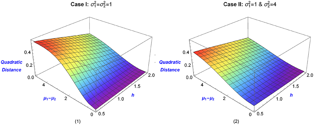
Figure 1. Quadratic Distances of two univariate normal distributions, as a function of the tuning parameter h and the mean difference μ1 − μ2. Graph (1) shows the distance between N(μ1, 1) & N(μ2, 1), while Graph (2) shows the distance between N(μ1, 1) & N(μ2, 4). Blue color corresponds to small distances (as measured by the magnitude of μ1 − μ2), with the change of color indicating a larger difference in means.
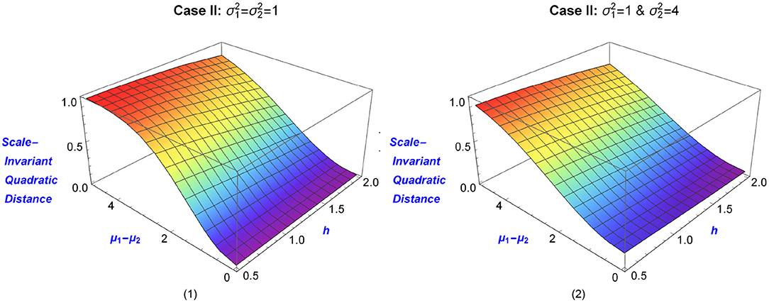
Figure 2. Scale-Invariant Quadratic Distances of two univariate normal distributions, as a function of the tuning parameter h and the mean difference μ1 − μ2. Graph (1) shows the distance between N(μ1, 1) & N(μ2, 1), while Graph (2) shows the distance between N(μ1, 1) & N(μ2, 4). Blue color corresponds to small distances (as measured by the magnitude of μ1 − μ2), with the change of color indicating a larger difference in means.
In the sequel, we take into account only the case of equal variances: , and we plot three distances as a function of the mean difference μ1 − μ2 (μ1 − μ2 ∈ [0, 5]). The solid lines in Figure 3 illustrate the scale-quadratic distance for two different values of the tuning parameter (h = 0.5 and h = 1). When the variances are equal, Equation (12) reduces to
The non-solid lines illustrated in Figure 3 represent the L1 distance (also known as total variation), which is given by the formula
and the scaled L2 distance, which, as mentioned before, can be derived from Equation (12) by setting h = 0.
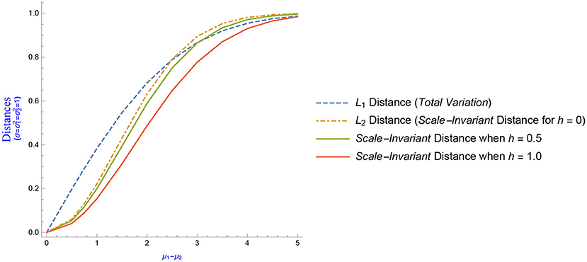
Figure 3. L1, L2 and Scale-Invariant Quadratic Distances between two univariate normal distributions N(μ1, 1) & N(μ2, 1), as a function of the mean difference μ1 − μ2.
The graphs illustrated in Figures 1–3 were created using the Wolfram Mathematica 11.1 program. For this purpose and in order to calculate the values of the depicted points, code was written in Wolfram Language by exploiting the formulae presented above.
In summary, the quadratic distance between two normal populations is an increasing function of the difference between the two parameter means when the two normal populations have equal variability. The shape of the distance does depend on the smoothing parameter that is selected by the user and provides different levels of smoothing, with higher values of h to correspond to greater smoothing. On the other hand, smaller values of h produce quadratic distances that are closer (in shape) to the L2 distance, for which h = 0.
The results presented in this section provide guidance on the performance of these distances in practical applications. The following section presents data examples with the purpose of illustrating these distances as evidence functions for model adequacy.
5. Illustrations and Examples
In this section, we present different examples using both simulated and real-world data with two or six dimensions. Our aim is to provide illustrations related to distances computed under different models so that the interested reader will get a better understanding on how the evidence functions and distances work in practice. Figures 4–6 and the numbers described in Table 1 were generated using the Wolfram Mathematica 11.1 program exploiting multivariate formulae analogous to the (univariate) ones presented in section 4.
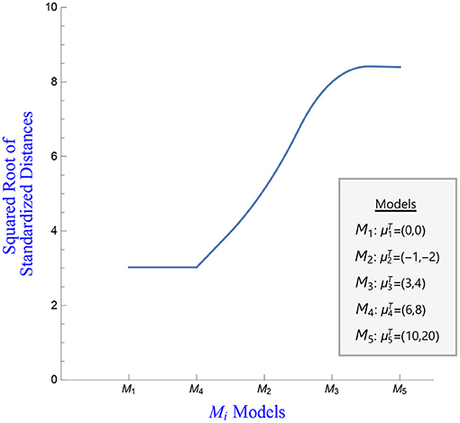
Figure 4. Squared root of the standardized estimates of the distances between model and the various fitted models.
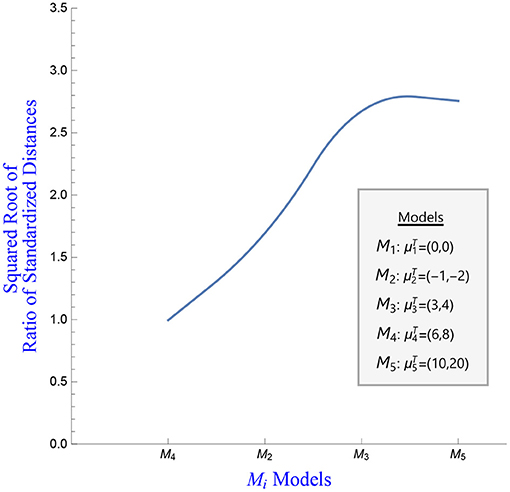
Figure 5. Squared root of the ratio of the standardized distance vs. the various fitted models.
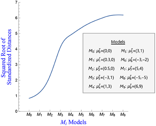
Figure 6. Squared root of the standardized estimates of the distances between model and the various fitted models.
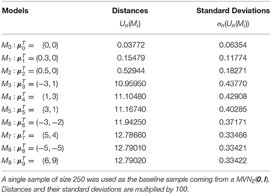
Table 1. Estimates of the distances for ten different models and their associated standard deviations.
5.1. Example # 1
The purpose of this illustration is to understand the behavior of quadratic distances as measures of evidence for model adequacy in various data structures arising when experimental data are generated.
We generate a single sample of size n = 400 from a mixture of two bivariate normal distributions as follows; 200 data points follow a bivariate normal distribution with mean 0 and covariance matrix I (abbrev. MVN2(0, I)). Another 200 data points are generated form a bivariate normal with the same covariance matrix I and mean μT = (6, 8). The different hypotheses postulate that the data are from models Mi, i = 1, 2, 3, 4, 5, where M1 corresponds to a bivariate normal with mean and covariance matrix I and the remaining models are bivariate normal with covariance matrix I and corresponding means , , and . For each case, we compute an estimate of the distance , i = 1, 2, 3, 4, 5 denoted by Un(Mi) and its associated variance. The kernel used to carry out the computation is the density of a multivariate normal with mean the observation xj, j = 1, 2, …, n and covariance matrix h · I. We use h2 = 0.5.
Figure 4 plots the squared root of the standardized estimates of the quadratic distances between data expressed as and the various fitted models. The plot indicates that models M1 and M4 provide an equally good fit to the data (the corresponding standardized distances are equal to 0.032), with the other models providing a worse fit to the data. This is actually expected because 50% of the sample comes from a bivariate normal with mean vector 0 (model M1) and 50% of the sample comes from a bivariate normal with mean μ4 (model M4). The quadratic distance, interpreted as an evidence function, provides evidence that supports equally well the use of models M1 and M4.
Figure 5 presents a plot of the squared root of the standardized distance () vs. the models fitted. This second plot is analogous to the log-likelihood plot of a hypothesis of interest vs. other competing hypothesis. The likelihood function is graphed to provide visual impression of the evidence over the parameter space. In analogy, we plot the ratio of the square root of the standardized distance for the different hypothesis over the standardized distance of the hypotheses of interest. Given that a small distance provides evidence of the model fit, the greater the value of the aforementioned ratio the stronger the evidence against the hypotheses Hi, i = 2, …, 5. A ratio of approximately 1 indicates that both models are almost equally supported by the data, hence both hypotheses are approximately equally supported by the data, so the evidence does not indicate any preference for one hypothesis over the other. For example, the squared root of the standardized distance of model M4 vs. model M1 equals 0.995107, indicating that both models M4 and M1 are equally supported by the data. This is indeed the case since, by design, 50% of the data points come from MVN2(0, I) with the remaining 50% of the data coming from a MVN2(μ, I), where μT = (6, 8).
5.2. Example # 2
A second illustration of quadratic distances as evidence functions for model adequacy is provided below. We generate a single sample of size 250 from a MVN2(0, I). We use this single sample as our baseline data and fit ten different models to obtain estimates of the standardized distances. The fitted models have a covariance matrix I and corresponding means as follows: , , , , , , , , and . We use h2 = 0.5 and a normal kernel as before. Table 1 presents the estimates of the distances for the different models and their associated standard deviations.
Notice that when the mean of the fitted model is the estimate of the distance is close to 0 with a very small standard deviation. Further, the more different the means are, the bigger the value of the distance estimate. Figures 6, 7 plot the squared root of the standardized distance estimates and the standardized ratio distance estimates. Interpretation of these plots is similar to the ones presented before.
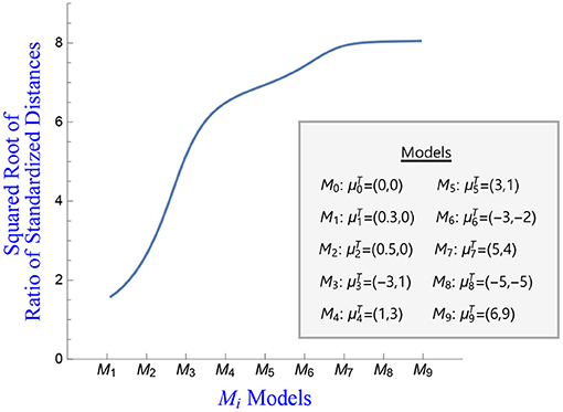
Figure 7. Squared root of the ratio of the standardized distance vs. the various fitted models.
5.3. Example # 3
This example uses a real experimental data set and illustrates that the quadratic distance evidence functions can be easily computed in higher than two dimensions and offer meaningful results. We use a multivariate data set introduced by Lubischew (1962). This data set contains three classes of Chaetocnema, a genus of flea beetles. Each class refers to a different type of species: Chaetocnema Concinna Marsh, Chaetocnema Heikertingeri Lubisch, and Chaetocnema Heptapotamica Lubisch of n1 = 21, n2 = 31 and n3 = 23 instances each. Six features/characteristics were measured from each species: the width of the first and the second joint of the first tarsus in microns (the sum of measurements for both tarsi), the maximal width of the aedeagus in the fore-part (in microns), the front angle of the aedeagus (1 unit = 7.5°), the maximal width of the head between the external edges of the eyes (in 0.01 mm), the aedeagus width from the side (in microns).
In this example, we take two of the chaetocnema species, Chaetocnema Heikertingeri Lubisch and Chaetocnema Heptapotamica Lubisch. Measurements are taken on six dimensions. There are 31 observations in the first group of species and 22 observations in the second group (Heptapotamica), in total 53 observations. To estimate the mean vector μi and the covariance matrix Σi for each group we use the maximum likelihood. Each group, therefore, is described by a six-dimensional normal distribution with corresponding means given as for the Heikertingeri species and for the Heptapotamica species with their associated covariance matrices. In this case, we use the models MVN6(0, I), MVN6(μHr, ΣHr) and MVN6(μHp, ΣHp) and computed their distance from the data set of 53 observations. Again, we used the multivariate normal kernel with h = 0.1. Notice that the standard multivariate normal model is also used in order to clearly indicate the difference in the values of the distance calculations. The fitting of the MVN6(μHr, ΣHr) and MVN6(μHp, ΣHp) offers estimators of the distance of 3.52 × 10⁻⁸ and 8.63 × 10⁻⁸, while the fitting of MVN6(0, I) gives a distance of 0.0005, indicating an estimate several orders of magnitude greater than the one obtained from the previous two cases. That is, the largest quadratic distance observed corresponds to the six-dimensional multivariate standard normal model. Furthermore, the squared root of the ratio of the standardized distances between the fitted Heptapotamica normal model (numerator) and the Heikertingeri normal model equals 1.57, implying that the evidence is inconclusive as to what model is supported. On the other hand, the corresponding quantities when the multivariate normal MVN6(0, I) model is used in the numerator and the Heptapotamica model is used in the denominator is 76.11, and when the Heikertingeri is used the corresponding ratio is 119.18, clearly indicating that the data does not support the MVN6(0, I) model.
6. Discussion and Conclusions
In this paper, we discuss the role of statistical distances as evidence functions. We review two definitions of evidence functions, one proposed by Lele (2004) and a second proposed by Lindsay (2004). We then examine the mathematical properties of some commonly used statistical distances and their suitability as evidence functions for model adequacy. Our investigation indicates that the class of the chi-squared distances and their extension, the class of quadratic distances introduced by Lindsay et al. (2008) and Lindsay et al. (2014) can be used as evidence functions for measuring model adequacy. This is because they can be interpreted as measures of risk, certain members of each class exhibit robustness properties, and if used as inference functions produce estimators that are asymptotically normal.
We propose also an explanatory analysis tool, namely the standardized distance ratio plot, that can be used to visualize the strength of evidence provided for, or against, hypotheses of interest and illustrate its use on experimental and simulated data. Our results indicate that quadratic distances perform well as evidence functions for measuring model adequacy. Furthermore, quadratic distances are of interest for a variety of reasons including the fact that several important distances are quadratic or they can be shown to be distributionally equivalent to a quadratic distance.
One of the reviewers raised the question of error probabilities associated with the use of statistical distances. Specifically, the reviewer asked whether the probabilities of misleading evidence and weak evidence are relevant in our context. We believe that measurement of model misspecification is an important step toward clarifying the suitability of a model class to explain the experimental data. However, we also think that a careful study of the behavior of these probabilities may shine additional light on distinguishing between different distances. The careful study of these questions is the topic of a future paper.
A second reviewer raised the question of potential connections of our work with work on the Focused Information Criterion (FIC) (Jullum and Hjort, 2017). The focus of our paper is on articulating the properties and illustrating, via data examples, the potential of statistical distances in assessing model adequacy. Connections with other model selection methods such as FIC will constitute the topic of future work. Finally, we would like to mention here that statistical distance concepts and ideas can be adapted to address model adequacy and model selection problems in many settings including linear, nonlinear and mixed effects models. Dimova et al. (2018) discuss in detail the case of linear regression and show that AIC and BIC are special cases of a general information criterion, the Quadratic Information Criterion (QIC).
Model assessment, that is, model adequacy and model selection is a fundamental and very important stage of any statistical analysis. Different techniques of model selection have been proposed in the literature describing how one could choose the best model among a spectrum of other competing models which best captures reality. However, provided that data were generated according to that specific model, the next logical step of a statistical analysis is to make statements about the study population. This implies making statistical inferences about the parameters of the chosen (data-dependent) model. Indeed, model selection strategies may have a significant effect or impact on inference of estimated parameters. Consequently, it is also crucial attention to be given to inference after model selection. For more information on estimation and inference after model selection, the interested reader is referred to Shen et al. (2004), Efron (2014), Fithian et al. (2017) and Claeskens and Hjort (2008, Chapters 6,7).
Data Availability Statement
Publicly available datasets were analyzed in this study. This data can be found here: https://www.jstor.org/stable/2527894?seq=1#metadata_info_tab_contents.
Author Contributions
MM developed the structure of the paper and contributed to writing of the paper. ES searched the literature and contributed to writing of the paper.
Funding
The authors acknowledge financial support from the Troup Fund, KALEIDA Health Foundation, award number 82114, in the form of a grant award to MM.
Conflict of Interest
The authors declare that the research was conducted in the absence of any commercial or financial relationships that could be construed as a potential conflict of interest.
References
Ahmad, I. A., and Cerrito, P. B. (1993). Goodness of fit tests based on the l2-norm of multivariate probability density functions. J. Nonparametr. Stat. 2, 169–181. doi: 10.1080/10485259308832550
Blume, J. D. (2002). Likelihood methods for measuring statistical evidence. Stat. Med. 21, 2563–2599. doi: 10.1002/sim.1216
Claeskens, G., and Hjort, N. L. (2008). Model Selection and Model Averaging. Cambridge: Cambridge University Press. doi: 10.1017/CBO9780511790485
Cox, D. R. (1990). Role of models in statistical analysis. Stat. Sci. 5, 169–174. doi: 10.1214/ss/1177012165
Cressie, N., and Read, T. R. (1984). Multinomial goodness-of-fit tests. J. R. Stat. Soc. Ser. B (Methodol.) 46, 440–464. doi: 10.1111/j.2517-6161.1984.tb01318.x
Dimova, R., Markatou, M., and Afendras, G. (2018). Model Selection Based on the Relative Quadratic Risk. Technical report, Department of Biostatistics, University at Buffalo, Buffalo, NY, United States.
Donoho, D. L., and Liu, R. C. (1988). Pathologies of some minimum distance estimators. Ann. Stat. 16, 587–608. doi: 10.1214/aos/1176350821
Efron, B. (2014). Estimation and accuracy after model selection. J. Am. Stat. Assoc. 109, 991–1007. doi: 10.1080/01621459.2013.823775
Fasano, G., and Franceschini, A. (1987). A multidimensional version of the KolmogorovSmirnov test. Month. Notices R. Astron. Soc. 225, 155–170. doi: 10.1093/mnras/225.1.155
Fithian, W., Sun, D., and Taylor, J. (2017). Optimal inference after model selection. arXiv:1410.2597v4 [math.ST].
Jullum, M., and Hjort, N. L. (2017). Parametric or nonparametric: the fic approach. Stat. Sin. 27, 951–981. doi: 10.5705/ss.202015.0364
Justel, A., Peña, D., and Zamar, R. (1997). A multivariate Kolmogorov-Smirnov test for goodness of fit. Stat. Probabil. Lett. 35, 251–259. doi: 10.1016/S0167-7152(97)00020-5
Lehmann, E. L. (1990). Model specification: the views of Fisher and Neyman, and later developments. Stat. Sci. 5, 160–168. doi: 10.1214/ss/1177012164
Lele, S. R. (2004). “Evidence functions and the optimality of the law of likelihood (with comments and rejoinder by the author),” in The Nature of Scientific Evidence, Statistical, Philosophical and Empirical Considerations, eds M. P. Taper and S. R. Lele (Chicago, IL: The University of Chicago Press), 191–216.
Lewin-Koh, N., Taper, M. L., and Lele, S. R. (2004). “A brief tour of statistical concepts,” in The Nature of Scientific Evidence, Statistical, Philosophical and Empirical Considerations, eds M. P. Taper and S. R. Lele (Chicago, IL: The University of Chicago Press), 3–16.
Li, B., and McCullogh, P. (1994). Potential functions and conservative estimating equations. Ann. Stat. 22, 340-356. doi: 10.1214/aos/1176325372
Lindsay, B. G. (1988). Composite likelihood methods. Contemp. Math. 80, 221–239. doi: 10.1090/conm/080/999014
Lindsay, B. G. (1994). Efficiency versus robustness: the case for minimum Hellinger distance and related methods. Ann. Stat. 22, 1081-1114. doi: 10.1214/aos/1176325512
Lindsay, B. G. (2004). “Statistical distances as loss functions in assessing model adequacy,” in The Nature of Scientific Evidence, Statistical, Philosophical and Empirical Considerations, eds M. P. Taper and S. R. Lele (Chicago, IL: The University of Chicago Press), 439–487.
Lindsay, B. G., and Markatou, M. (2002). Statistical Distances: A Global Framework to Inference. New York, NY: Springer.
Lindsay, B. G., Markatou, M., and Ray, S. (2014). Kernels, degrees of freedom, and power properties of quadratic distance goodness-of-fit tests. J. Am. Stat. Assoc. 109, 395–410. doi: 10.1080/01621459.2013.836972
Lindsay, B. G., Markatou, M., Ray, S., Yang, K., and Chen, S. C. (2008). Quadratic distances on probabilities: a unified foundation. Ann. Stat. 36, 983–1006. doi: 10.1214/009053607000000956
Lindsay, B. G., and Qu, A. (2000). Quadratic Inference Functions. Technical report, Pennsylvania State University.
Lubischew, A. A. (1962). On the use of discriminant functions in taxonomy. Biometrics 18, 455–477. doi: 10.2307/2527894
Markatou, M., Basu, A., and Lindsay, B. G. (1998). Weighted likelihood equations with bootstrap root search. J. Am. Stat. Assoc. 93, 740–750. doi: 10.1080/01621459.1998.10473726
Markatou, M., and Chen, Y. (2018). Non-quadratic distances in model assessment. Entropy 20:464. doi: 10.3390/e20060464
Markatou, M., Chen, Y., Afendras, G., and Lindsay, B. G. (2017). “Statistical distances and their role in robustness,” in New Advances in Statistics and Data Science, eds D. G. Chen, Z. Jin, G. Li, Y. Li, A. Liu, and Y. Zhao (New York, NY: Springer), 3–26.
Peacock, J. A. (1983). Two-dimensional goodness-of-fit testing in astronomy. Month. Notices R. Astron. Soc. 202, 615–627. doi: 10.1093/mnras/202.3.615
Royall, R. M. (2000). On the probability of observing misleading statistical evidence (with discussion). J. Am. Stat. Assoc. 94, 760–780. doi: 10.1080/01621459.2000.10474264
Royall, R. M. (2004). “The likelihood paradigm for statistical evidence,” in The Nature of Scientific Evidence, Statistical, Philosophical and Empirical Considerations, eds M. P. Taper and S. R. Lele (Chicago, IL: The University of Chicago Press), 119–152.
Shen, X., Huang, H.-C., and Ye, J. (2004). Inference after model selection. J. Am. Stat. Assoc. 99, 751–762. doi: 10.1198/016214504000001097
Sober, E. (2008). Evidence and Evolution: The Logic Behind the Science. Cambridge: Cambridge University Press.
Taper, M. L., and Lele, S. R. (2004). “The nature of scientific evidence: a forward-looking synthesis,” in The Nature of Scientific Evidence, Statistical, Philosophical and Empirical Considerations, eds M. P. Taper and S. R. Lele (Chicago, IL: The University of Chicago Press), 527–551.
Keywords: evidence functions, inference, kernels, model selection, quadratic and non-quadratic distances, statistical distances, statistical loss measures
Citation: Markatou M and Sofikitou EM (2019) Statistical Distances and the Construction of Evidence Functions for Model Adequacy. Front. Ecol. Evol. 7:447. doi: 10.3389/fevo.2019.00447
Received: 17 February 2019; Accepted: 06 November 2019;
Published: 22 November 2019.
Edited by:
Jose Miguel Ponciano, University of Florida, United StatesReviewed by:
Nils Lid Hjort, University of Oslo, NorwaySubhash Ramkrishna Lele, University of Alberta, Canada
Copyright © 2019 Markatou and Sofikitou. This is an open-access article distributed under the terms of the Creative Commons Attribution License (CC BY). The use, distribution or reproduction in other forums is permitted, provided the original author(s) and the copyright owner(s) are credited and that the original publication in this journal is cited, in accordance with accepted academic practice. No use, distribution or reproduction is permitted which does not comply with these terms.
*Correspondence: Marianthi Markatou, markatou@buffalo.edu