Patterns and Drivers of UV Absorbing Chromophoric Dissolved Organic Matter in the Euphotic Layer of the Open Ocean

Introduction

A fraction of the DOM in the oceans, termed colored DOM (CDOM), is optically active, absorbing light in the ultraviolet (UV) and blue bands of the light spectrum, with absorbance decreasing exponentially toward longer wavelengths (Morel and Maritorena, 2001). CDOM is formed of a complex mixture of organic compounds of terrestrial and marine origin (Coble, 2007; Mostofa et al., 2013; Nelson and Siegel, 2013; Stedmon and Nelson, 2015). Autochthonous sources of CDOM in the euphotic layer of the open ocean include primary producers (Nelson et al., 1998; Romera-Castillo et al., 2010; Fukuzaki et al., 2014), microzooplankton (Strom et al., 1997), zooplankton (Steinberg et al., 2004; Urban-Rich et al., 2006; Ortega-Retuerta et al., 2009), and bacterioplankton (Kramer and Herndl, 2004). Advection (Siegel et al., 2002; Nelson et al., 2007, 2010; Nelson and Siegel, 2013) and vertical mixing (Højerslev et al., 1996; Bracchini et al., 2010; Yamashita et al., 2013) also impact the distribution of CDOM in the ocean surface layer. Although allochthonous terrestrial inputs have a major effect on the distribution of CDOM in coastal areas (Miller and Moran, 1997; Blough and Del Vecchio, 2002; Chen et al., 2004; Coble, 2007), they also contribute to the open ocean CDOM (Andrew et al., 2013; Cartisano et al., 2018). These authors provided evidences that CDOM in Equatorial Atlantic and North Pacific waters is composed of a major terrestrial component. This terrestrial DOM is largely derived from degradation products of lignins (Spencer et al., 2009), possibly tannins and other hydroxyl-(methoxy) and polyhydroxy-aromatic compounds.

Chromophoric dissolved organic matter has received attention because it is the major factor controlling the attenuation of UV radiation and also contributes to attenuate the PAR in the illuminated ocean (Kirk, 1994; Zepp et al., 2007). CDOM is highly photo-reactive, being degraded upon exposure to solar radiation (Mopper et al., 2015). In fact, the main abiotic sink of CDOM in the open ocean is photobleaching (Siegel and Michaels, 1996; Nelson and Siegel, 2001; Del Vecchio and Blough, 2002; Zhang et al., 2009). This process involves the transformation of CDOM into smaller, low MW and less colored molecules (e.g., hydrocarbons, aldehydes, ketones, organic acids) or into inorganic carbon (CO and CO₂), and nutrient salts (NH₄⁺ and HPO₄^2-) (Mopper et al., 1991; Miller and Zepp, 1995; Moran and Zepp, 1997; Moran et al., 2000). Thereby, photobleaching increases the underwater light penetration and, thus, the depth of the photic layer (Mopper et al., 2015). Conversely, solar radiation can also lead to an increase of CDOM through the transformation of biogenic organic compounds, such as triglycerides or the amino acid tryptophan, into more complex aromatic humic-like substances through photohumification (Kieber et al., 1997; Berto et al., 2016). Therefore, the distribution of CDOM in the open ocean is the result of the balance between biogeochemical sources, e.g., photohumification and biogeneration, and sinks, e.g., photobleaching and microbial utilization (Romera-Castillo et al., 2011), together with the physical effect of water mass advection and mixing.

The plethora of studies that describe the optical properties of CDOM in the open ocean have been chiefly focused on the calibration of sensors installed on satellites (Carder et al., 1989; Siegel et al., 2005; Fichot et al., 2008; Morel and Gentili, 2009; Swan et al., 2013) and on the study of light penetration in the ocean (Morel and Prieur, 1977; Johannessen et al., 2003; Tedetti and Sempéré, 2006; Zepp et al., 2007). Whereas the importance of CDOM in ocean biogeochemical cycles is well documented (Mopper et al., 1991; Zepp, 2003; Zepp et al., 2007; Reader and Miller, 2011), analyses based on extensive in situ CDOM spectral measurements are thus far limited for the upper layer of the ocean (Nelson et al., 1998, 2004), being more extensively analyzed in the dark ocean (Nelson et al., 2010; Nelson and Siegel, 2013; Catalá et al., 2015). Open ocean concentrations of CDOM are difficult to estimate due to their low absorption levels, particularly at the upper photic layer of the tropical and subtropical open oceans.

There is an assortment of proxies including different absorption coefficients, spectral slopes and other indices broadly applied in the literature to quantify and characterize CDOM (Twardowski et al., 2004; Helms et al., 2008; Loiselle et al., 2009). More recently, novel approaches to model the spectral properties of CDOM based on separating the exponential decay signal due to humic substances from the spectral shoulders due to other chromophores have been proposed (Röttgers and Koch, 2012; Massicotte and Markager, 2016). The spectral slopes of CDOM in the ranges of 275–295 nm (S_275-295) and 350–400 nm (S_350-400) are widely applied to reveal MW differences and/or the effect of photobleaching (Helms et al., 2008). The absorption coefficient ratio at 254/365 nm, (a_254/365) has also been proven to be a useful proxy for the average MW of CDOM (Dahlen et al., 1996; Engelhaupt et al., 2003). High values of a_254/365 indicate lower average MW compounds (Berggren et al., 2010). The absorption coefficient at a₂₅₄ frequently exhibits a positive linear relationship with the bulk DOC concentration (Weishaar et al., 2003) since conjugated double bonds are one of the most abundant forms of carbon in the DOM pool. This linear relationship has been observed in coastal waters influenced by river plumes (Chen et al., 2011; Spencer et al., 2012) or by continental runoff (Spencer et al., 2009), as well as in open waters of the temperate Eastern North Atlantic (Lønborg and Álvarez-Salgado, 2014) and the Mediterranean Sea (Catalá et al., 2018). Given that very few solar photons of wavelength < 295 nm reach the Earth’s surface (Fichot and Benner, 2011), a₂₅₄ should not be directly influenced by the incident solar UV radiation (Del Vecchio and Blough, 2002). Conversely, the absorption coefficient at 325 nm (a₃₂₅), which represents the aromatic fraction of CDOM, does respond to the absorption of the solar UVA radiation and, therefore, it represents the balance between microbial production and photochemical degradation of this CDOM pool (Nelson et al., 2004).

Such a variety of indices and calculations render comparisons among studies challenging, so that a globally coherent in situ assessment of CDOM properties in the upper layer of the open ocean is still lacking. Here we address this gap by reporting the distribution of CDOM in the euphotic open ocean along the Malaspina 2010 Circumnavigation Expedition (Duarte, 2015), that sampled the tropical Atlantic, Indian, and Pacific Oceans. We aimed to assess the physical and biogeochemical drivers that control the CDOM distribution by firstly comparing CDOM amount and quality indices across the 15 Longhurst’s biogeographic provinces visited. Secondly, we explore the relationships between the different CDOM indexes and nine physical and biogeochemical parameters characterizing the tropical and subtropical euphotic ocean.

Materials and Methods

Cruise Track and Sample Collection

The Malaspina 2010 circumnavigation sailed the subtropical and tropical ocean on board of R/V Hesperides, from the 16th of December 2010 to the 14th of July 2011 (Supplementary Table S1). The expedition occupied a total of 147 hydrographic stations along the Atlantic, Indian, and Pacific oceans, between 40° S and 35° N (Figure 1), including fifteen Longhurst’s biogeographic provinces (Longhurst, 1995, 1998), as classified following Catalá et al. (2016).

FIGURE 1

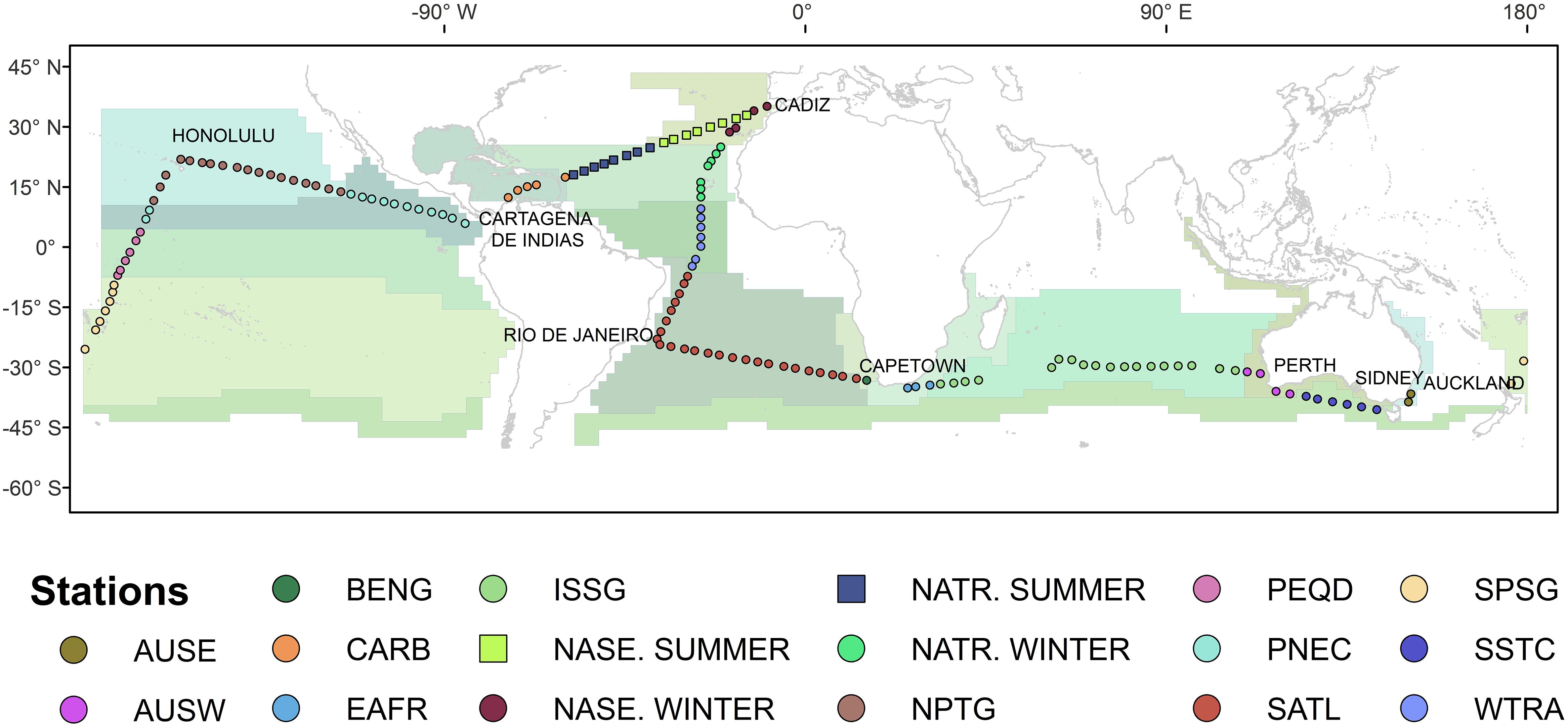
Figure 1. Map of the biogeographic provinces with the 147 stations crossed during Malaspina 2010 expedition. The positions of the stations sampled between 35° N and 40° S are marked with circles. Different colors of the circles indicate the different 15 biogeographic provinces, parceled by Longhurst’s classification (1995, 1998, 2007). AUSE, East Australian Coastal Province; AUSW, Australia-Indonesia Coastal Province; BENG, Benguela Current Coastal Province; CARB, Caribbean Province; EAFR, E. Africa Coastal Province; ISSG, Indian S. Subtropical Gyre Province; NASE, N. Atlantic Subtropical Gyral Province; NATR, N. Atlantic Tropical Gyral Province, NPTG, N. Pacific Gyre Province; PEQD, Pacific Equatorial Divergence Province; PNEC, N. Pacific Equatorial Countercurrent Province; SATL, South Atlantic Gyral Province; SPSG, S. Pacific Subtropical Gyre Province; SSTC, S. Subtropical Convergence Province; WTRA, Western Tropical Atlantic Province. Note the different colors for the same province NASE and NATR, crossed both in winter and in summer. (For more details see Catalá et al., 2016 and Supplementary Table S1).

Water samples were collected through the surface layer up to the DCM. A rosette sampler with 24 Niskin bottles of 12 l was dipped at each station at about 10:00 a.m. (local time) and five nominal depths were sampled according to the profile of PAR. They were 70, 50, 20, 7% PAR and the DCM. The percentage of PAR received at the DCM depth during the study corresponded to 2.9% ± 0.4 (mean ± SE).

The rosette sampler was equipped with a CTD probe Seabird 911, a polarographic membrane oxygen sensor Seabird SBE43, a fluorometer Seapoint and a radiometer Biospherical/Licor to continuously obtain the vertical profiles of salinity (S), potential temperature (𝜃), dissolved oxygen (O₂), in vivo fluorescence of chlorophyll a (FISP) and PAR, respectively. Temperature and pressure sensors were calibrated at the SeaBird laboratory before the circumnavigation. On board, salinity calibration was carried out daily with a Guildline AUTOSAL model 8410B salinometer (Pérez-Hernández et al., 2012), the oxygen sensor was calibrated daily (in μmol kg^-1) with the potentiometric end-point Winkler method (Álvarez et al., 2012) and the fluorescence of Chl a profiles were calibrated by fluorimetry (in mg m^-3) as in Estrada (2012).

Measuring and Processing CDOM Spectra

A total of 700 water samples were collected to record their absorption coefficient spectra of CDOM. They were poured from the Niskin bottles into 125 mL acid-washed glass flasks and stored in the dark to equilibrate at room temperature until measurement within 2–3 h of collection. Aliquots of 50 mL were gently filtered through a 0.2 μm pore size Millex filter (PTFE membrane), in order to remove cells and particles, by means of a syringe, avoiding the development of bubbles. The initial 20 mL were used to flush the syringe and the filter and the remaining 30 mL to fill the quartz cuvette. Absorption measurements were performed immediately after filtration.

The UV-visible absorption spectra of CDOM were collected between 250 and 750 nm at 1 nm intervals in 10-cm path length quartz cuvettes in a double beam Perkin Elmer lambda 850 spectrophotometer. Fresh UV-milli-Q water was used as blank. The mean absorbance from 600 to 750 nm was subtracted from all absorbance measurements to correct the residual scattering caused by micro-air bubbles or colloidal material present in the sample, refractive index differences between the sample and the reference, or light attenuation that was not related to organic matter. The estimated detection limit of the spectrophotometer is 0.001 absorbance units.

The absorbance at any wavelength was converted into Naperian absorption coefficient a_λ (in m^-1) using the equation:

$$\begin{array}{c}{a}_{\text{λ}} = 2.303\frac{[AB{S}_{\text{λ}} - AB{S}_{600--750}]}{l}\left(1\right)\end{array}$$

where ABS_λ is the absorbance at wavelength λ, ABS_600-750 is the average absorbance between 600 and 750 nm, l is the path length of the cuvette (0.1 m) and 2.303 is the factor that converts from decadic to natural logarithms. Given that the detection limit of the instrument in Naperian absorption coefficient units is 0.02 m^-1, we took as reliable a_λ measurements those above 0.05 m^-1, i.e., about 3 times the detection limit. This means that, given the limitations of our instrument, we discarded the visible part of the absorption spectra (wavelengths > 370 nm) and focus on the UV part.

On this basis, three optical parameters recurrently used in the literature were chosen as proxies to describe the variability in the amount (a₂₅₄, a₃₂₅) and quality (a_254/365) of CDOM. As explained in the introduction, there is not a consensus absorption coefficient wavelength for the fluorescent visible chromophores. In this work, we decided to use a₃₂₅ for three reasons. Firstly, to allow direct comparison of our results with Nelson and collaborators, who always report a₃₂₅ in their reference papers about CDOM in open ocean waters (e.g., Nelson et al., 1998, 2004, 2010). Secondly, because a₃₂₅ represents the absorption of marine humic-like marine compounds (Ex/Em, 320 nm/410 nm) better than any other wavelength. And thirdly, it is sufficiently away for 370 nm, the wavelength at which absorption measurements are within the detection limit in our instrument. Furthermore, following Helms et al. (2008), a CDOM spectral slope was calculated over the narrow wavelength range 275–295 nm, S_275-295, using linear regressions of the natural log-transformed a_λ spectra. This range is identified as one of the most dynamic regions of the natural log transformed absorption spectra (Helms et al., 2013) and appears to be particularly sensitive to shifts in MW or DOM origin (Helms et al., 2008). Thus, together with the CDOM spectral slope over 350–400 nm, S_350-400, it is commonly applied as a tool for the structural characterization of CDOM. Steeper slopes indicate a faster decrease in absorption with increasing wavelength, which are inversely correlated to the MW and directly correlated to photobleaching of CDOM. Helms et al. (2008) also proposed a dimensionless parameter, the S_R, which is the ratio between, S_275-295 and S_350-400. However, S_350-400 and S_R were not calculated because of the limitations of our instrument. In any case, the assortment of indices and spectral slopes that will be used in the range 250–370 nm, will provide new insights on CDOM variability in the open tropical and subtropical ocean.

Companion Measurements and Calculations

From the salinity (S) and potential temperature (𝜃) at each sampling depth, we calculated derived variables such as the thermal, haline and total stratification. The thermal and haline stratification were calculated from the gradients of potential temperature and salinity (Δ𝜃 and ΔS) over the upper 150 m as the difference between the potential temperature or salinity at 150 m and the shallowest CTD depth (3–6 m) and divided by the difference in depth (z). Therefore, negative values of Δ𝜃 and positive values of ΔS indicate stratified waters. Total stratification was quantified by the squared Brunt-Väisäla frequency (N², in min^-2) calculated following Millard et al. (1990) between the surface and 150 m.

Apparent oxygen utilization, in μmol kg^-1, was calculated as the difference between the saturation and the measured dissolved oxygen concentrations. Dissolved oxygen saturation was derived from practical salinity and potential temperature applying the equation of Benson and Krause (1984). Inorganic nutrients, and particularly Nitrate (NO₃^-), in μmol kg^-1, were determined on board using standard segmented flow analysis with colorimetric detection (Blasco et al., 2012).

Picophytoplankton abundance of Prochlorococcus (Proc), Synechococcus (Syn) and eukaryotic picoautotrophs (EUK) were determined on board in fresh samples by flow cytometry following Lubián (2012) as detailed in Agusti et al. (2019). BB was also determined by flow cytometry using standard protocols (Gasol and del Giorgio, 2000). A previously published calibration curve relating relative side scatter to cell size (Calvo-Díaz and Morán, 2006) was used to transform the cytometric signal and cell size was converted to biomass using the Gundersen et al. (2002) relationship.

Daily, weekly and monthly shortwave solar radiation, SWR (wavelength range, 175–3850 nm, reported in MJm^-2d^-1), were obtained from the National Centre for Environmental Predictions NCEP/DOE 2 reanalysis database provided by the NOAA/OAR/ESRL PSD, Boulder, CO, United States, from their website at http://www.esrl.noaa.gov/psd/ and interpolated for each location of the CTD stations cruise.

ANOVA Analysis

To evaluate the intra- and inter-province variability, and differences among PAR levels for each environmental and optical parameter, analyses of variance (ANOVA) were performed. The provinces AUSE, BENG, EAFR and NASE_W (see caption of Figure 1 for acronyms) were excluded because they comprised less than 5 stations. To further assess the individual differences among provinces and PAR levels, Tukey post hoc tests were performed after the ANOVAs.

Generalized Additive Models

Generalized Additive Models (GAMs, Wood, 2006) were used to test for the effect of the environmental parameters on the variability of CDOM parameters. A GAM is a non-parametric regression technique that allows inspecting the relationship between a response variable and one (or more) explanatory variable(s) without the need to choose a particular parametric form for describing the shape of the relationship(s). The assortment of environmental drivers to be tested (SWR, S, 𝜃, N², ΔS, Δ𝜃, O₂, NO₃^-, AOU, Chl a, Proc, Syn, EUK, and BB) on each CDOM parameter were first analyzed using VIFs to evaluate their covariance. After this analysis, we excluded N², O₂, NO₃^- and EUK from the analysis as VIFs values were above and acceptable cut-off level of 3 (Zuur et al., 2010). A cut-off level is a selected threshold used to evaluate covariability when calculating VIFs. Therefore, we finally tested a total of 10 candidate predictor variables: SWR, S, 𝜃, ΔS, Δ𝜃, AOU, Chl a, Proc, Syn and BB (Supplementary Table S2). GAMs were formulated as follows:

$$\begin{array}{c}{Y}_{i,l} = \text{α} + {\displaystyle \sum _j }{g}_j (X_{i,l}^j) + {\text{ε}}_{i,l}\left(2\right)\end{array}$$

where Y is the CDOM optical variable (a₂₅₄, a₃₂₅, a₂₅₄/a₃₆₅, S_275-295) measured at a station i and nominal level l, α is the intercept and X is a vector of predictor variables where the superscript j identifies each covariate. g are non-parametric smoothing functions specifying the effect of the covariates on the optical variable and 𝜀_i,l is the error term assumed to be normally distributed. Smoothing functions were fit by penalized cubic regression splines restricted to a maximum of three knots. The smoothness of the functions was estimated by minimizing the gcv criterion and only statistically significant covariates were retained in the final optimal formulations. For the ten explanatory variables tested (see above) all were retained but BB. Weekly SWR was selected among the daily, weekly and monthly SWR options on basis of minimizing the AIC and the gcv. For each individual explanatory variable, we estimated the relative importance using the ‘pvmd’ metric as implemented in the ‘relaimpo 2.2-3’ package (Grömping, 2006), and calculating gcv score changes when deleting covariates sequentially and one at a time while keeping the rest.

Chl a Proc and Syn were ln-transformed, and depth was included in all models as a “catch-all” variable to account for potential unmeasured effects on CDOM parameters. All models were fitted in R 3.5.1 software (R Development Core Team, 2018) and using the ‘mgcv 1.8-27’ package (Wood, 2006).

Results

Physical and Biogeochemical Variability Along the Circumnavigation

The distributions of potential temperature, salinity, dissolved oxygen and fluorescence of Chl a recorded by the sensors attached to the rosette sampler (Figure 2) helped us to define the biogeographic provinces occupied during the circumnavigation (Catalá et al., 2016). Temperature showed homogeneous profiles in some biogeographic provinces such as the North Atlantic Subtropical Gyre in summer (NASE_S), the SSTC and the NPTG, and highly stratified in others, such as the NASE in winter (NASE_W), the WTRA, the PEQD, and the PNEC (Supplementary Figure S2). Salinity was also vertically homogeneous in some provinces as SSTC, EARF and the North Atlantic Tropical Gyre in summer (NATR_S) (Supplementary Figure S3) whilst showing a pronounced gradient in others such as WTRA, PNEC and the CARB (Figure 2B). AOU expanded over a wide range of values (-29.0 to 257.8 μmol kg^-1) from the highly productive surface layer of coastal upwelling systems (BENG) to the aged subsurface waters of the equatorial pacific (PNEC). AOU increased significantly with depth in all provinces, being always positive at the depth of the DCM, except in SSTC (Figure 2C and Supplementary Figure S4). Minimum values of Chl a were found in the center of the oceanic subtropical gyres of the North and South Atlantic (NATR and SATL) and the Indian (ISSG) oceans, whereas the maximum value of 1.71 mg m^-3 was found at the DCM of NPTG (Figure 2D and Supplementary Figure S5). The depth of the DCM ranged from 37 to 159 m, with an average ± SD of 101 ± 31 m. The maximum depth was found in NATR_S whereas the minimum occurred at PNEC, i.e., in the equatorial upwelling of the Pacific Ocean (Figure 3D and Supplementary Figure S1).

FIGURE 2

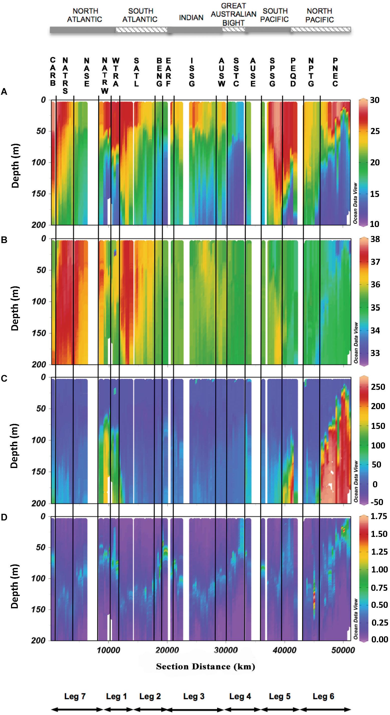
Figure 2. Vertical depth profiles of hydrographic CTD continuum parameters among the biogeographic provinces crossed during the circumnavigation (see caption of Figure 1 for acronyms): (A) potential temperature 𝜃 (°C), (B) Salinity (S), (C) Apparent oxygen utilization (AOU) (μmol kg^-1), and (D) Chlorophyll a (Chl a) (mg m^-3).

FIGURE 3

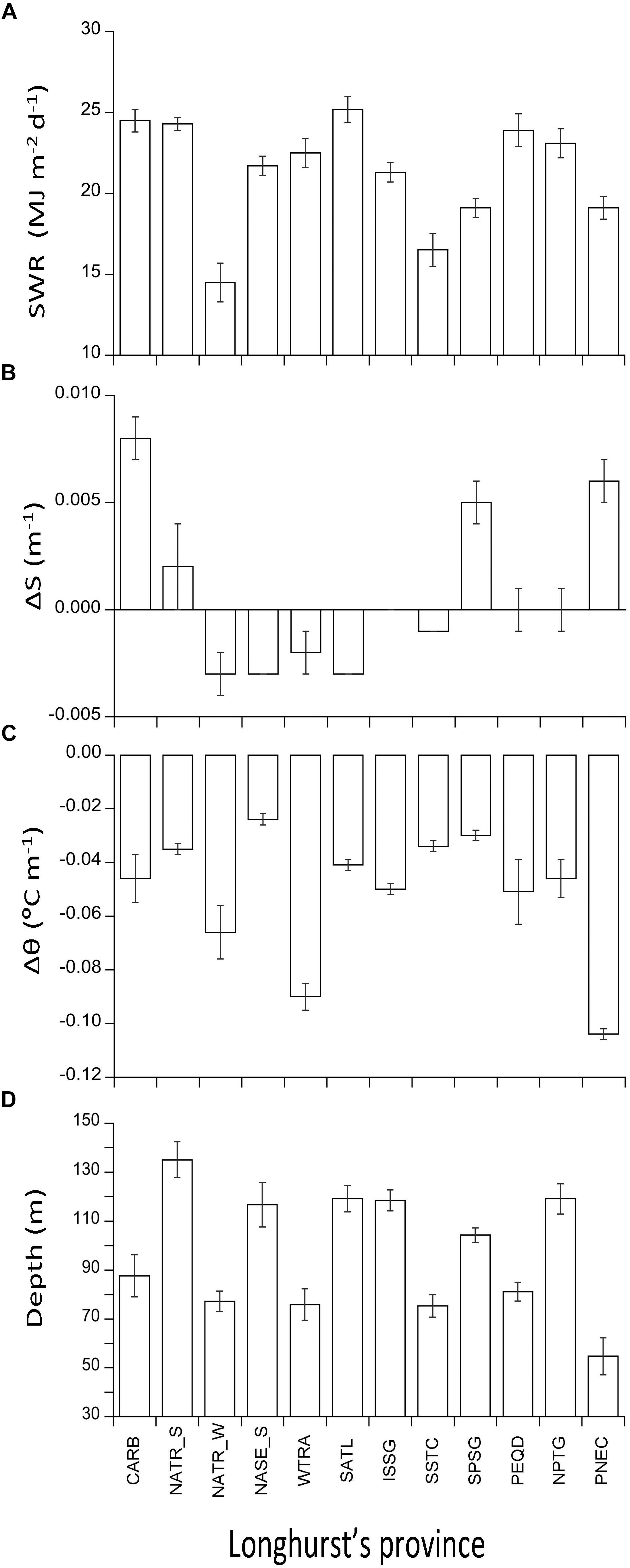
Figure 3. Bar plots of the distribution of selected explanatory variables (average ± SD): (A) weekly shortwave radiation SWR (MJ m^-2 d^-1), (B) Gradient of salinity, DS (m^-1), (C) Gradient of temperature, D𝜃 (°C m^-1), and (D) Depth of the DCM (m) among biogeographic provinces. Note that (B–D) are integrated with depth.

Differences Among Biogeographic Provinces

The weekly average shortwave radiation (SWR) along the cruise ranged from 11.1 MJ m^-2d^-1 in the North Atlantic gyre crossed in winter (NATR_W) to 31.0 MJ m^-2d^-1 in the South Atlantic gyre (SATL), crossed in summer (Figure 3A). The average gradient of salinity (ΔS) was 0.00037 ± 0.0039 m^-1, ranging from -0.0054 m^-1 in NATR_W to WTRA to 0.0122 m^-1 in PNEC and CARB (Figure 3B). The gradient of potential temperature (Δ𝜃) ranged from -0.115°C m^-1 to -0.010°C m^-1 in PNEC and NPTG, respectively (Figure 3C). The combination of the vertical profiles of Δ𝜃 and ΔS defines which provinces are more or less stratified.

The warmest of all provinces crossed during the circumnavigation was CARB, with a mean temperature of 28.05°C and a 25–75% IQR of 27.61–28.80°C. Only PEQD, SPSG (South Pacific Subtropical Gyre) and WTRA were as warm as CARB (Figures 4A, 5, p < 0.05). Conversely, the coldest province was SSTC, with a mean temperature of 16.95°C and an IQR of 15.69–18.44°C (Figure 4A), which was significantly colder than all the other provinces (Figures 4A, 5, p < 0.05). The saltiest province was NASE_S, with mean salinity of 37.04 and an IQR of 36.76–37.37, whilst the fresher province was PNEC, with mean salinity of 34.18 and an IQR of 33.94–34.50 (Figure 4B). Overall, significant differences were observed between almost all provinces (Figure 5). The highest AOU was found in PNEC, with a mean of 43.8 μmol kg^-1 and a wide IQR from -4.9 to 70.9 μmol kg^-1. The lowest AOU was found in SATL, with a mean of -9.4 μmol kg^-1 and a narrow IQR from -13.4 to -7.9 μmol kg^-1 (Figure 4C). When comparing the AOU of provinces with each other, no significant differences were observed, except for PNEC (and SATL with NPTG) (Figure 5). The province with the highest Chl a was PNEC, with a mean of 0.49 mg m^-3 and an IQR of 0.31–0.64 mg m^-3, whilst the province with the lowest Chl a crossed during the circumnavigation was the Indian South Subtropical Gyre (ISSG), with a mean of 0.14 mg m^-3 and a IQR of just 0.06–0.15 mg m^-3 (Figure 4D). Also, when comparing among provinces for Chl a, PNEC was different from all the other provinces except with WTRA (Figure 5). The distributions of Proc and Syn are not presented here because they have been recently reported by Agusti et al. (2019), who found the highest abundances of Proc in NATR and SSTC, although Syn was more abundant in PNEC and SSTC. Both populations showed the lowest abundance in the Indian South Subtropical Gyre (ISSG) (Agusti et al., 2019).

FIGURE 4

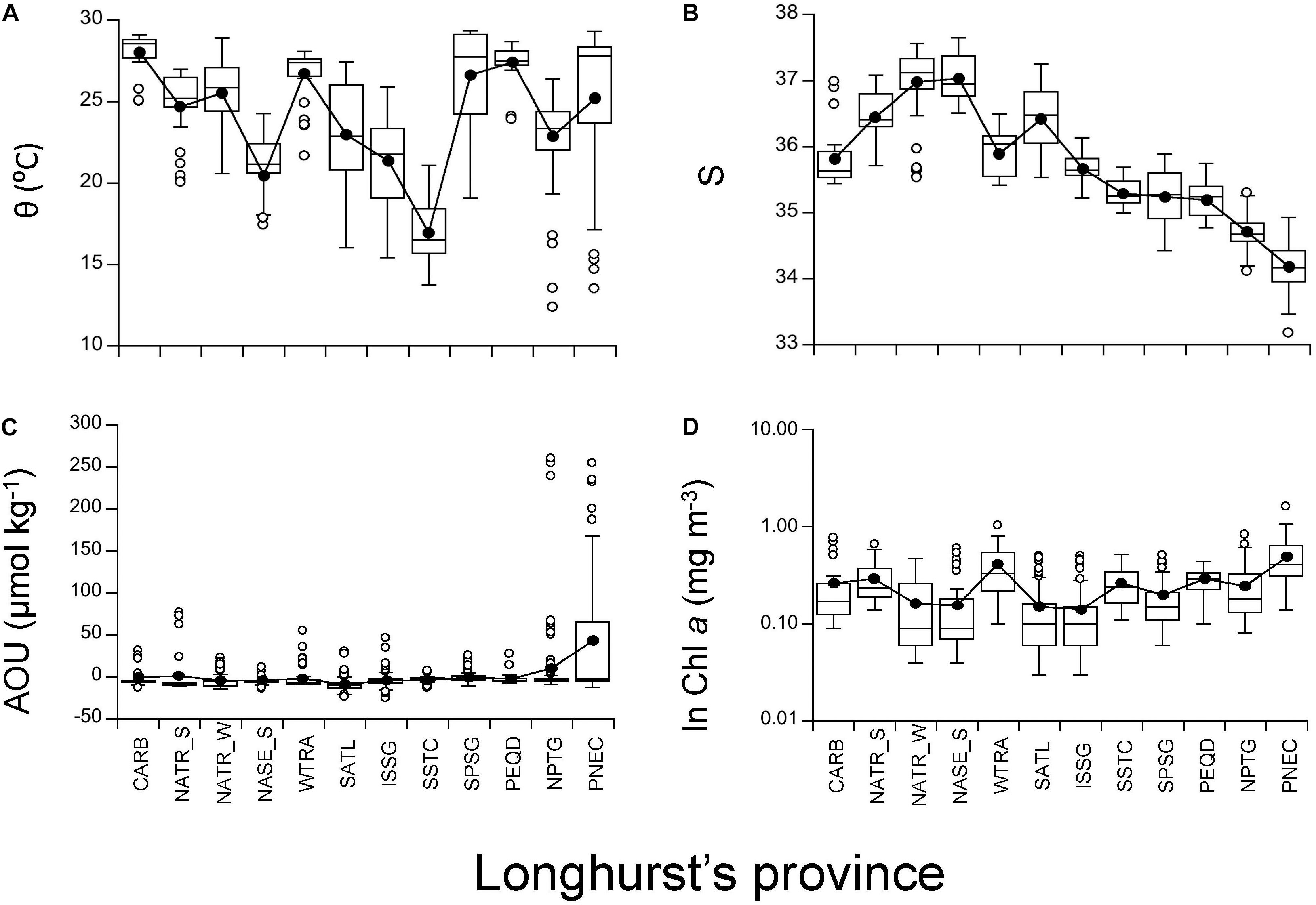
Figure 4. Box and Whisker plots applied to the four physical, chemical and biological explanatory variables at each biogeographic province. Horizontal line represents median; black circles represent means; white-box represent 25–75% percentiles and whiskers extend from the upper (lower) to the highest (lowest) value that is within 1.5x inter-quartile range of the hinge. Solid black line connects all mean values for each Longhurst’s province among the oceans. (A) Potential temperature, (B) Salinity, (C) AOU, and (D) Chl a. Note that Chl a was ln-transformed.

FIGURE 5

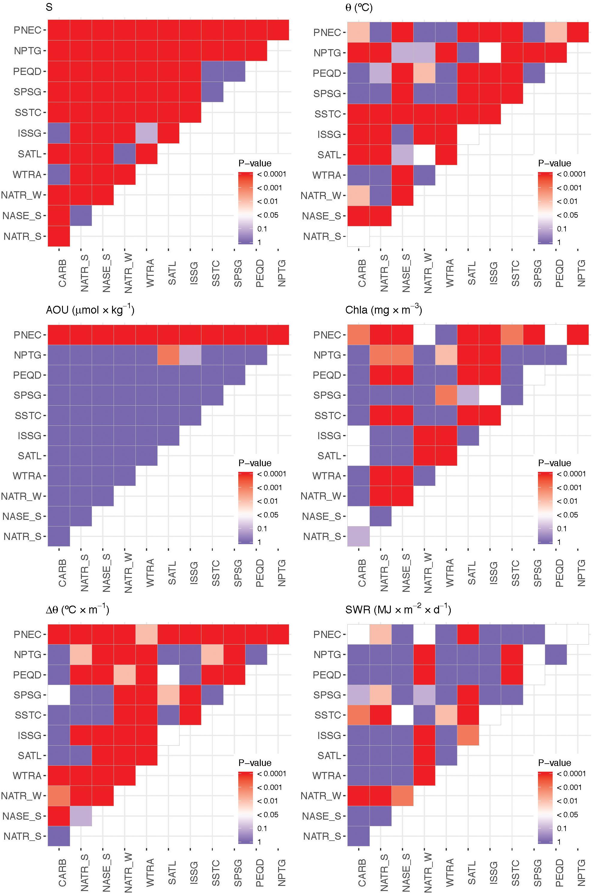
Figure 5. P-value of the F-statistic test resulted from the ANOVA applied to the six environmental variables (Δ𝜃, SWR, S, 𝜃, AOU and Chl a), to evaluate inter-province variability.

Differences With PAR Level

Potential temperature ranged between the highest global mean of 24.79 ± 3.12°C (IQR, 22.63–27.42°C) at the surface and the lowest mean of 20.56 ± 3.82°C (IQR, 17.39–23.53°C) at the DCM, respectively (Figure 6A). Salinity was rather homogeneous with the lowest global mean of 35.64 ± 0.93 (IQR, 34.98–36.33) at the 20% level of PAR (mean depth, 38 ± 11 m) and the highest mean of 35.77 ± 0.79 (IQR, 35.23–36.33) at the DCM (Figure 6B). AOU (Figure 6C) and Chl a (Figure 6D) increased as PAR levels decreased with depth and ranged from the highest global mean of 22.39 ± 52.59 μmol O₂ kg^-1 (IQR, 0.35–18.48 μmol O₂kg^-1) and 0.47 ± 0.24 mg Chl a m^-3 (IQR, 0.33–0.51 mg Chl a m^-3) at the DCM and the lowest global mean of -5.84 ± 5.39 μmol O₂kg^-1 (IQR from -8.77 to -4.02 μmol O₂kg^-1) and 0.16 ± 0.13 mg Chl a m^-3 (IQR, 0.07–0.21 mg Chl a m^-3) at the surface, respectively. There were not significant differences in salinity among PAR levels, AOU was significantly different only at the DCM, and 𝜃 and Chl a at the DCM and the 7% PAR (Supplementary Figure S10). As described in Agusti et al. (2019), Proc and Syn abundance showed a weak but significant trend to increase with Chl a concentration, and a stronger tendency to increase with temperature and PAR. The abundance of picocyanobacteria increased with increasing percent PAR until PAR reached > 10% and showed a tendency for a slight decline at PAR levels > 30% surface irradiance.

FIGURE 6

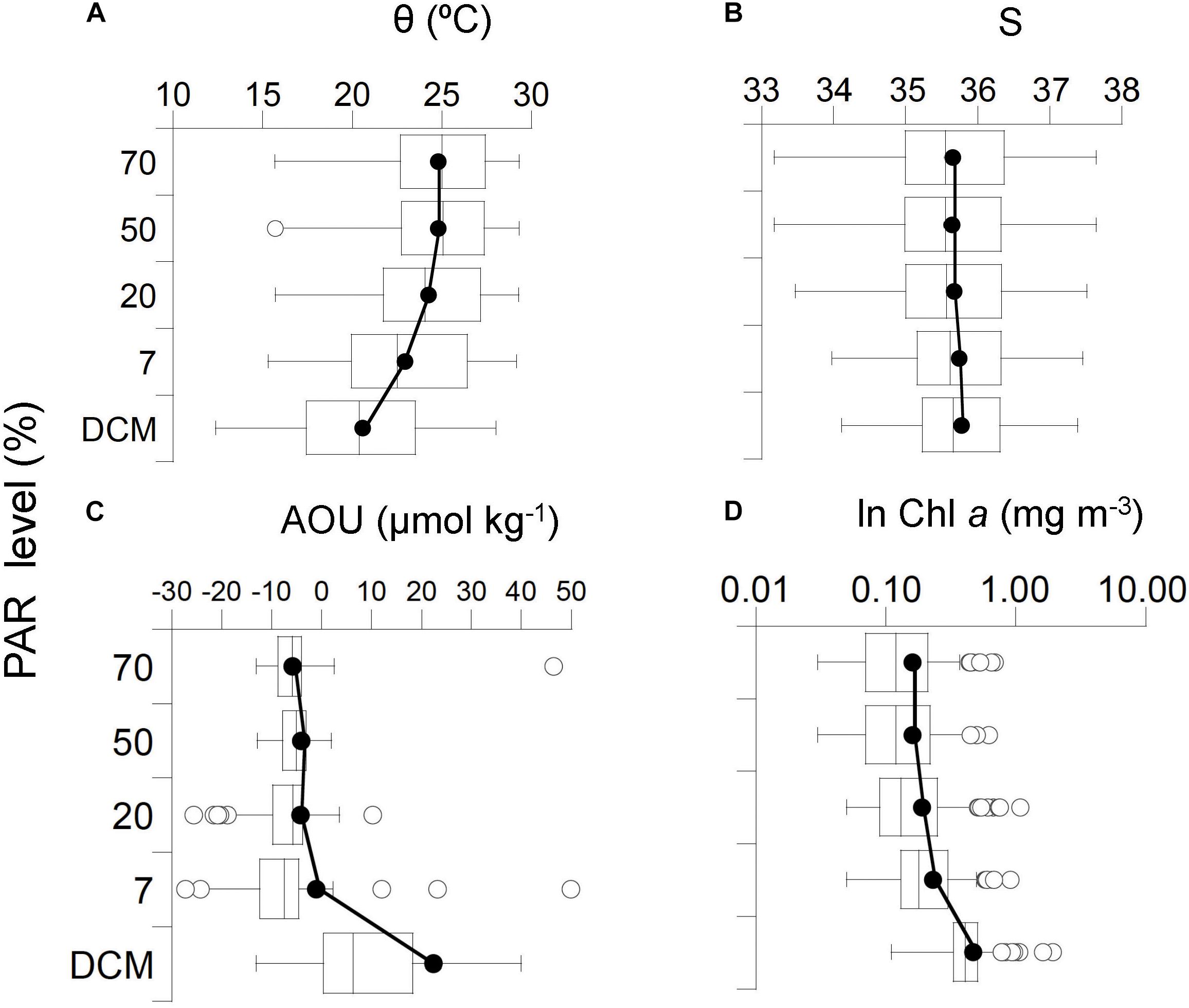
Figure 6. Box and Whisker plots representing average global distribution among the photic layer (five nominal depths) of the physical, chemical and biological explanatory variables: (A) Potential temperature 𝜃, (B) Salinity S, (C) Apparent oxygen utilization AOU, and (D) Chlorophyll a. Note that Chl a was ln-transformed. Horizontal line represents median; black circles represent means; white-box represent 25–75% percentiles and whiskers extend from the upper (lower) to the highest (lowest) value that is within 1.5x inter-quartile range of the hinge. Solid black line connects global mean values within the photic layer.

CDOM Variability Along the Circumnavigation

Differences Among Biogeographic Provinces

Among all the provinces crossed during the circumnavigation, the oligotrophic gyres were characterized by significantly lower a₂₅₄ and a₃₂₅ coefficients (ANOVA F = 107.5, 590 DF, p < 0.0001 for a₂₅₄ and F = 42.14, 590 DF, p < 0.0001 for a₃₂₅) with the ISSG province presenting the lowest values and the equatorial upwelling PNEC province the highest values (Figure 7A and Supplementary Figure S6). The mean value of a₂₅₄ was 1.12 m^-1 (IQR, 1.05–1.17 m^-1) in ISSG and 1.64 m^-1 (IQR, 1.46–1.79 m^-1) in PNEC (Figure 7A). Mean a₃₂₅ was 0.10 m^-1 (IQR, 0.07–0.14 m^-1) in ISSG and 0.33 m^-1 (IQR, 0.24–0.43 m^-1) in PNEC (Figure 7B and Supplementary Figure S7). Coherently, the a_254/365 quality ratio was significantly higher in the oligotrophic gyres (F = 21.9, 590 DF, p < 0.0001; Figure 7C and Supplementary Figure S8). In general, this ratio changed among biogeographic provinces, from the lowest mean of 10 (IQR, 6–13) in PNEC to the highest mean of 32 (IQR, 24–37) in NATR_S (Figure 7C). The UV spectral slope S_275-295 ranged from the lowest mean of 30.02 μm^-1 (IQR, 23.49–35.47 μm^-1) in the PNEC province to the highest mean of 47.19 μm^-1 (IQR, 41.26–53.09 μm^-1) in the ISSG province (Figure 7D and Supplementary Figure S9), with the subtropical gyres presenting significantly higher values (ANOVA F = 37.81, 590 DF, p < 0.0001). Further, the Indian Ocean province was significantly (p < 0.001) different from all the others for all the optical parameters (Figure 8). Conversely, the biogeographic provinces of the Pacific Ocean (including the South Australia convergence, SSTC province) were significantly different from the rest of the provinces showing significantly higher a₃₂₅ coefficient (ANOVA F = 156.7, 590 DF, p < 0.0001) and lower UV spectral slope S_275-295 (ANOVA, F = 160.2, 590 DF, p < 0.0001), despite the highest values measured across the study were found in the South Pacific Subtropical Gyre (SPSG, Figure 7).

FIGURE 7

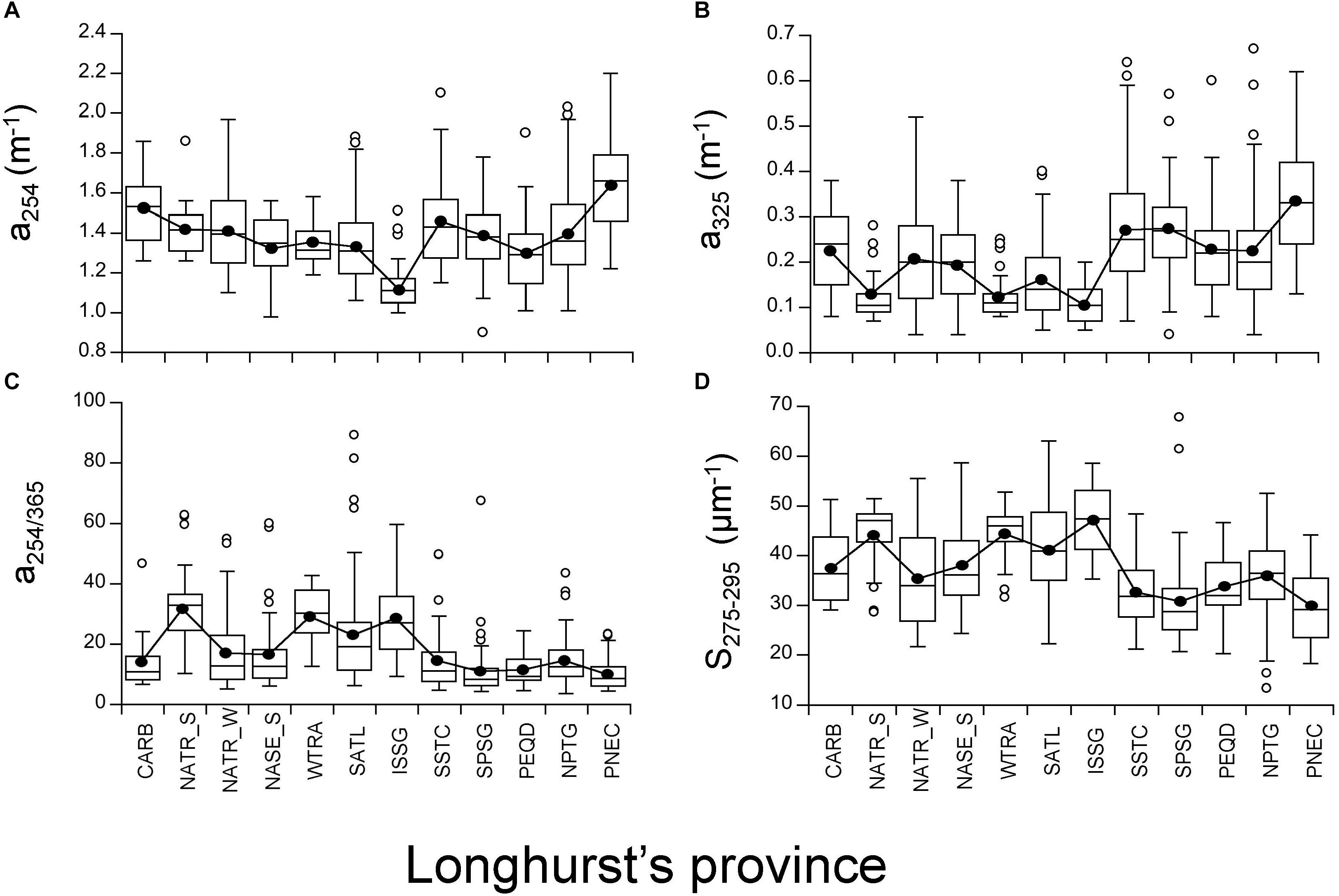
Figure 7. Box and Whisker plots for the four explained optical variables at each biogeographic province. Horizontal line represents median; black circles represent means; white-box represent 25–75% percentiles and whiskers extend from the upper (lower) to the highest (lowest) value that is within 1.5x inter-quartile range of the hinge. Solid black line connects all mean values for each province among the oceans. (A) a₂₅₄, (B) a₃₂₅, (C) a_254/365, and (D) S_275-295.

FIGURE 8

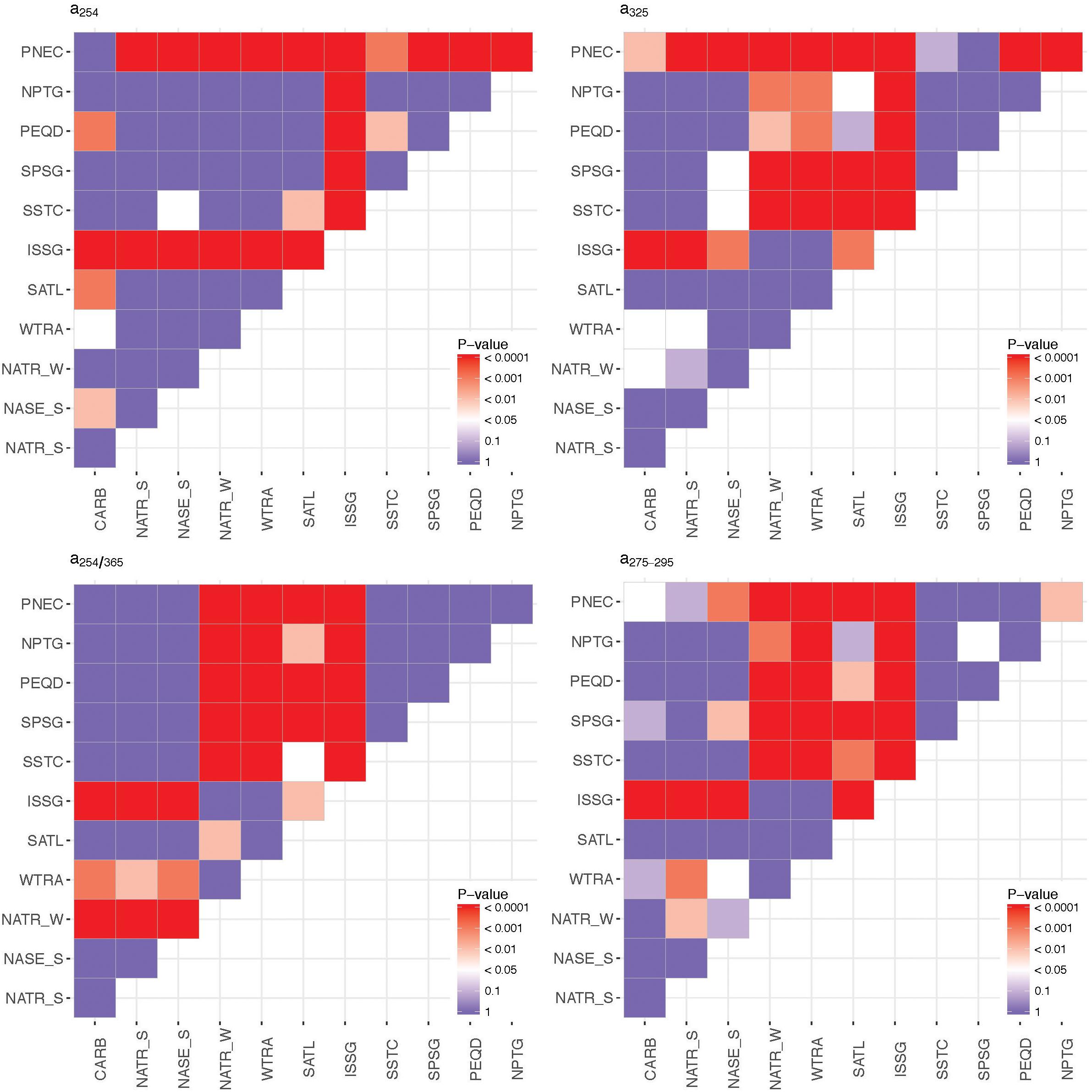
Figure 8. P-value of the F-statistic resulted from the ANOVA applied to the four optical variables a₂₅₄, a₃₂₅, a_254/365, S_275-295 to evaluate inter-province variability.

Differences With PAR Level

Overall, the vertical profiles of a₂₅₄ did not reveal significant variability as a function of PAR levels, except between 7 and 70% PAR (Supplementary Figure S11), and showed a global mean value of 1.36 ± 0.23 m^-1 (IQR, 1.19–1.49 m^-1) (Figure 9A and Supplementary Figure S6). This suggests that photochemical decomposition at this wavelength is not a primary driver of CDOM variability. Otherwise, we detected a significant increase of a₃₂₅ as a function of the PAR levels from the lowest global mean of 0.14 ± 0.08 m^-1 (IQR, 0.08–0.20 m^-1) at the surface to the highest of 0.26 ± 0.13 m^-1 (IQR, 0.15–0.33 m^-1) at the DCM depth (Figure 9B and Supplementary Figures S7, S11). Consistently, the lowest global mean of the CDOM quality ratio a_254/365 of 12.96 ± 8.29 (IQR, 7.15–16.48) was found at the DCM and reached the highest global mean of 25.83 ± 15.83 (IQR, 13.35–34.35) at the surface (Figure 9C). The UV slope S_275-295 values exhibited the lowest mean of 32.4 ± 7.9 μm^-1 at the DCM (IQR, 26.1–38.5 μm^-1) and the highest mean of 42.9 ± 8.8 μm^-1 at the surface (IQR, 35.8–49.6 μm^-1) (Figure 9D). Overall, significant differences between PAR levels were observed for all optical variables, except a₂₅₄ (Supplementary Figure S11), showing the largest differences when comparing the surface and DCM layers. When analyzing the biogeographic provinces individually, differences in the vertical distribution of the absorption coefficients were observed in the provinces where stratification occurs while in those where mixing conditions prevail, like in SSTC, profiles of a₂₅₄ and a₃₂₅ were more homogeneous (Supplementary Figures S6, S7).

FIGURE 9

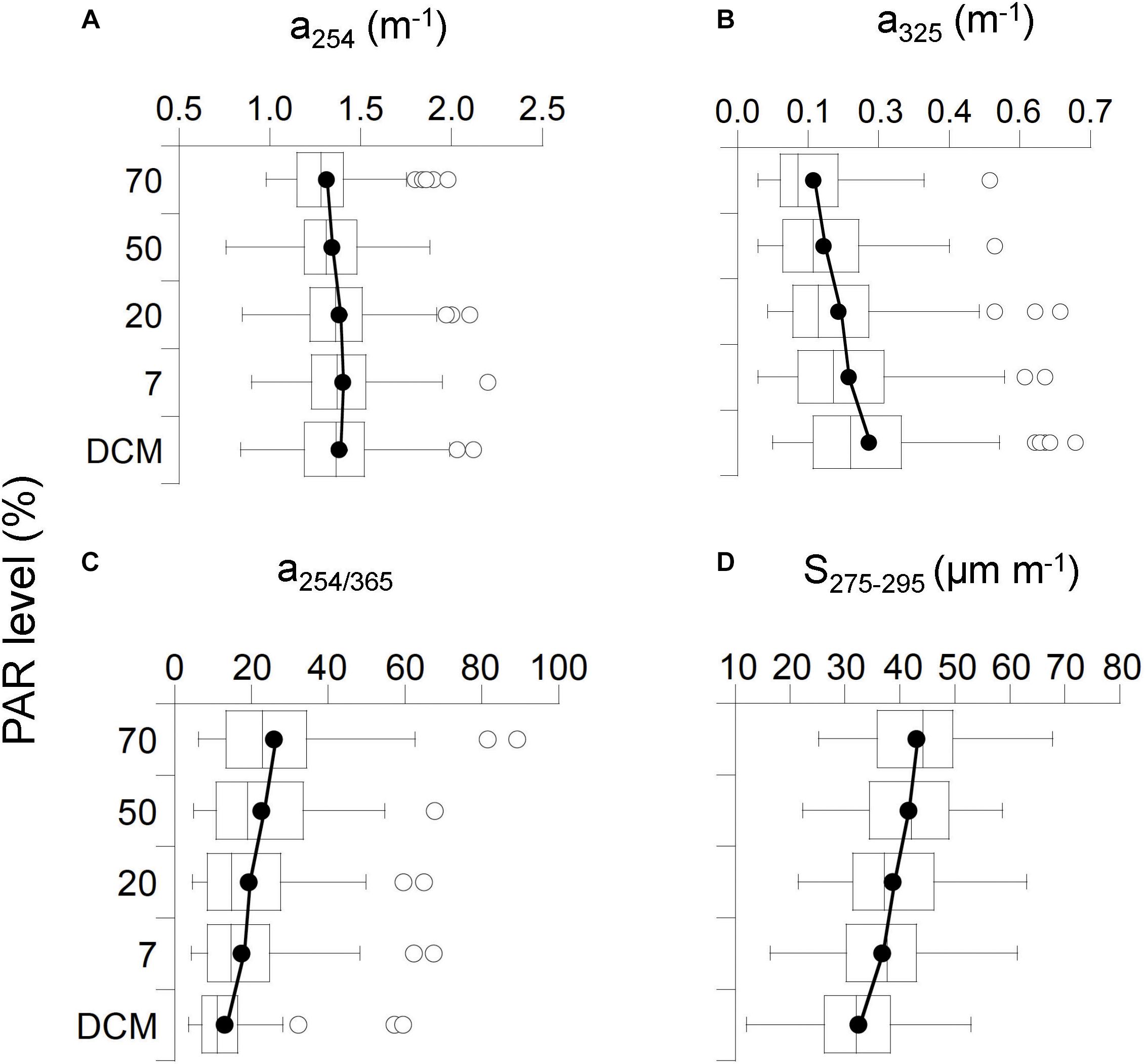
Figure 9. Box and Whisker plots representing average global distribution among the photic layer (five nominal depths) of the optical explained variables: (A) a₂₅₄, (B) a₃₂₅, (C) a_254/365, and (D) S_275-295. Horizontal line represents median; black circles represent means; white-box represent 25–75% percentiles and whiskers extend from the upper (lower) to the highest (lowest) value that is within 1.5x inter-quartile range of the hinge. Solid black line connects global means values within the photic layer.

Linking Optical and Environmental Parameters

Generalized additive models were used to explore the physical and biogeochemical factors that drive the global distribution of optical parameters in the photic layer of the tropical and subtropical open ocean (Figure 10). The total deviance explained by the models for a₂₅₄, a₃₂₅, a_254/365 and S_275-295 was 32, 41, 40, and 49% respectively (Supplementary Table S3). In all instances, BB was not a significant variable (p > 0.05) thus excluded from the final formulations. Interestingly, the direction of the effects (with the exception of AOU) differed from a₂₅₄ and a₃₂₅ to a_254/365 and S_275-295 (Figure 10). The covariates that mainly explained the variability of a₂₅₄ were Chl a, Syn, ΔS and AOU (according to pmvd in Supplementary Table S3), although removing Proc from the model could have a great impact too (Supplementary Table S3). The relationships with Chl a and Syn were nearly linear, whilst that with AOU was inverse. The relationship with ΔS was non-linear and started to be positive at positive values of the haline gradient (Figure 10). a₃₂₅ was explained by all the explanatory variables tested. Chl a, ΔS, AOU and S were the main explanatory variables (Supplementary Table S3). Biogeochemical drivers such as Chl a and AOU showed positive linear and non-linear relationships, respectively. Physical drivers such as S and ΔS showed an inverse and linear relationship until around 35.5 and 0.0, respectively. It should also be highlighted the positive relationship with Syn, as for the case of a₂₅₄. The most important covariate that governs the a_254/365 ratio was again Chl a, showing a nearly inverse relationship (Figure 10). Interestingly, Proc showed an inverse relationship for abundances below 6 × 10⁴ cells mL^-1 and a direct relationship for abundance above that threshold (Figure 10), being this covariate an important contributor to the deviance explained in this model (Supplementary Table S3). The relationship with physical drivers such as 𝜃 and S was non-linear, although a positive linear increase was observed until a threshold around 20°C and 35.5, respectively. Consequently, the relationship of a_254/365 with the gradients of 𝜃 and S decreased as a function of stratification. Finally, solar radiation also contributes to explain the global a_254/365, although through an apparently counterintuitive inverse relationship (Figure 10). The UV slope S_275-295 was explained by all the explanatory variables. The most important drivers were essentially the same drivers than for the a_254/365 ratio (Supplementary Table S3). In this case, it should be highlighted the nearly linear and reverse relationship with Syn, and again this covariate was an important contributor to the deviance explained by this model (Supplementary Table S3).

FIGURE 10

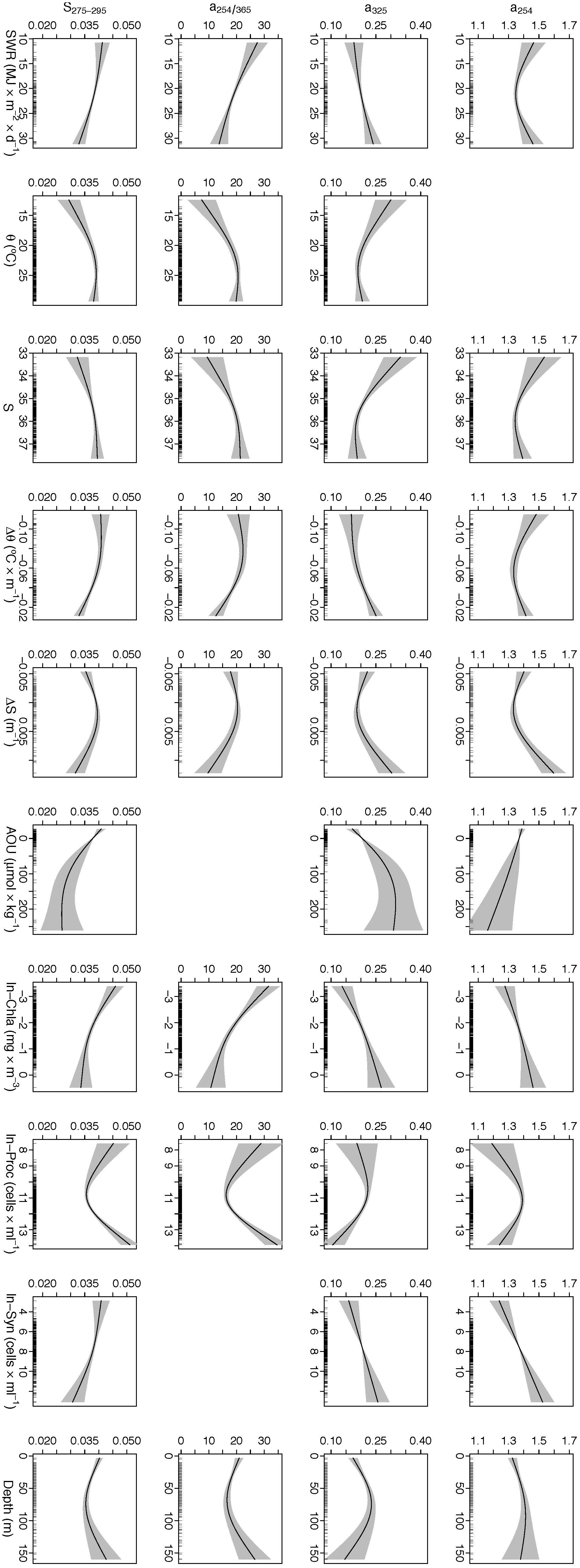
Figure 10. Partial plots derived from GAMs showing the additive effects of the physical, chemical and biological factors on the optical variables. Black lines represent the smoothing functions and the gray shaded areas represent 95% point-wise confidence intervals. Rugs (ticks) on x-axis indicate the distribution of the data.

Discussion

CDOM Extremes in the Tropical and Subtropical Epipelagic Open Ocean

The majority of the Longhurst’s biogeographic provinces sailed during the Malaspina 2010 circumnavigation are located in tropical and subtropical oligotrophic regions. Particularly, the most oligotrophic province intercepted during the expedition was the ISSG as revealed by its low Chl a concentration (Figure 4D and Supplementary Figure S5), deepness of the DCM (Figure 2D) and low CDOM absorption in the UV range of the spectrum (Figures 7A,B). Specifically, at this province we found the lowest CDOM absorption values (Figure 7B and Supplementary Figure S7). Coherently, Catalá et al. (2016) reported that the waters with the lowest fluorescence of CDOM were also found in ISSG. These results improve our current knowledge on the optical properties of these waters, since no previous data were available so far apart from the latitudinal section made by Nelson et al. (2010). According to the present literature, the lowest CDOM values in the epipelagic zone of the world ocean are expected for the eastern South Pacific Subtropical Gyre (SPSG), described as the most UV transparent oceanic waters (Bricaud et al., 2010; Morel et al., 2010; Tedetti et al., 2010), which was not visited during the Malaspina 2010 circumnavigation. Otherwise, we visited some provinces characterized by higher Chl a levels, due to the influence of upwelling systems like the equatorial upwelling provinces WTRA and PNEC (Figure 4D and Supplementary Figure S5). The BENG and EATR coastal upwelling provinces were also sampled during the Malaspina 2010 expedition although they were not included in our analysis as they contain less than 5 stations each (Figure 1 and Supplementary Table S1). Particularly, PNEC was the most singular biogeographic province crossed during the circumnavigation, exhibiting unique hydrographic properties, because of the influence of the equatorial upwelling forced by the trade winds and the Pacific countercurrent that transports eastwards the warm water masses of the Western Pacific, against the mean tropical trade wind forces (Schmitz, 1996). In PNEC we found the most stratified waters of all the circumnavigation and the maximum AOU and CDOM absorption coefficient values were observed. Interestingly, a₃₂₅ in the other equatorial upwelling province, WTRA, was as low as in ISSG. This can be explained by the higher SWR and lower AOU in WTRA compared with PNEC.

Chlorophyll a as a Driver of CDOM Variability in the Surface Open Ocean

Overall, when we gathered our data independently of the biogeographic provinces, Chl a was found to be the most significant biogeochemical driver of CDOM variability in the euphotic layer of the open ocean that we tested (Supplementary Table S3). Indeed, satellite data indicate that the global distribution of CDOM at 443 nm exhibits similar patterns to the distribution of Chl a (e.g., Siegel et al., 2002). In our case, both a₂₅₄ and a₃₂₅ show a positive linear relationship with Chl a (Figure 10). Given that phytoplankton support most of the primary production of organic matter in the open ocean (Falkowski et al., 1998, 2003), a positive correlation between CDOM and Chl a is expected. In this sense, phytoplankton acts as a direct source of CDOM (e.g., Romera-Castillo et al., 2010; Fukuzaki et al., 2014) and also acts as an indirect source because the extracellular release of DOM, cell lysis or grazing processes trigger the heterotrophic activity. In fact, a plethora of studies have already demonstrated the role of grazers (Strom et al., 1997; Steinberg et al., 2004; Urban-Rich et al., 2006; Ortega-Retuerta et al., 2009), virus (Suttle, 2007) and bacteria (Nelson and Siegel, 2001; Rochelle-Newall and Fisher, 2002; Kramer and Herndl, 2004; Nelson et al., 2004) as indirect producers of CDOM. Hence, Chl a traces both the autotrophic and heterotrophic processes contributing to the production of CDOM in the epipelagic ocean. It should be noted too that both Proc and Syn contribute to explain CDOM indices (Figure 10). Particularly, Syn abundance is linear and positively related to both a₂₅₄ and a₃₂₅. The relatively low total explained variance of the absorption indices explained by the GAM models (32–49%; Supplementary Table S3) are likely related to the analytical limitations of the absorption measurements rather than to any environmental driver that we had not tested. Note that the RMSE of the GAM models is 0.09 m^-1 for a₃₂₅, just four times the detection limit and twice the estimated measurement error.

AOU as a Driver Pointing That a₂₅₄ and a₃₂₅ Represent Different CDOM Pools

The AOU in the photic layer represents the cumulative net community respiration, i.e., the autotrophic production of dissolved oxygen minus the respiration by all autotrophs and heterotrophs (Kirchman, 2012). Therefore, negative values of AOU indicate net phytoplankton production and positive values indicate net community respiration. Our results show that a₂₅₄ and a₃₂₅ present an opposite relationship with AOU in the photic layer, suggesting different CDOM pools. On the one side, a₂₅₄ presents an inverse relationship with AOU (Figure 10). Note that the shape of the relationship between a₂₅₄ and AOU does not change in the surroundings of AOU = 0 μmol kg^-1. Therefore, it is not necessary to analyze the samples with negative AOU separately from those with positive AOU. Given that a₂₅₄ reflects the amount of conjugated carbon double bonds, it is expected that it can work as a proxy of DOC not only in coastal (Weishaar et al., 2003) but also in open ocean waters (Lønborg and Álvarez-Salgado, 2014; Catalá et al., 2018). In this sense, an inverse relationship has been observed between DOC and AOU both in the euphotic (Pan et al., 2014) and the dark ocean (Aristegui et al., 2002; Hansell et al., 2009).

Conversely, a₃₂₅ shows a positive linear relationship with AOU (Figure 10). As for the case of a₂₅₄, the relationship between a₃₂₅ and AOU does not change around AOU = 0 μmol kg^-1. Given that the absorption at 325 nm is due to aromatic compounds (Coble, 1996; Jørgensen et al., 2011), the positive relationship with AOU suggests that a₃₂₅ is a tracer for the production of the aromatic humic-like materials that absorb at 320–340 nm and fluoresce at 400–450 nm during the microbial degradation of organic matter (Coble, 1996; Jørgensen et al., 2014; Catalá et al., 2016). Therefore, a₃₂₅ could be considered a tracer of the MCP, which postulates the production of refractory DOM as a consequence of the processing of bioavailable organic matter in the oceans (Ogawa et al., 2001; Jiao et al., 2010; Goto et al., 2017).

Maximum CDOM values were found at the DCM, where the AOU maximum is also found (Supplementary Figure S4), which also coincide with Chl a maximum for the global tropical and subtropical ocean examined in this study, indicating that biological processes are the major autochthonous source of CDOM in the open epipelagic ocean. Previous studies in the Sargasso Sea (Nelson et al., 1998, 2004) and across the NASE and SATL Atlantic provinces (Kitidis et al., 2006) also identified the largest CDOM levels at the DCM zone.

Photobleaching, the Abiotic Counter Partner

The third driver governing the CDOM patterns in the epipelagic layer was solar radiation (Figure 10). The incidence of solar ultraviolet radiation is not equally distributed globally, as the Southern Hemisphere is receiving consistently higher radiation than the Northern (Herman, 2010). There is also seasonal variability, although we expect low influence because the circumnavigation was run in spring and summer (Duarte, 2015). This must influence the potential photobleaching of the surface layer across the different provinces. Yet, oligotrophic tropical and subtropical regions are exposed to high penetration of solar radiation (Tedetti et al., 2007), resulting in enhanced photobleaching rates. The UV slope S_275-295 has been proposed as a tracer of the photobleaching history in the open ocean (Yamashita et al., 2013). The UV slope values described in the literature for oceanic areas ranged between 10 and 30 μm^-1 with a defined pattern of increase with decreasing depth up to 20 and 60 μm^-1, plausibly due to photobleaching. Our values are in accordance with these data ranges reported by Stedmon and Nelson (2015). It is remarkable that the highest values of S_275-295 were found in the ISSG province during the Malaspina 2010 circumnavigation, suggesting that the subtropical waters of the Indian Ocean were the most exposed to photobleaching. By contrast, the Pacific Ocean provinces showed significantly lower values of S_275-295, indicating a lower impact of photobleaching on the distribution of CDOM in those waters (Figure 8).

The vertical variability of a_254/365 (Figures 9B,C) also points to photobleaching in SW. Two opposite processes act on this ratio throughout the photic layer: on the one side the biogeneration of CDOM, higher at the DCM, due to autotrophic production and microbial respiration (Nelson et al., 1998, 2004; Rochelle-Newall and Fisher, 2002), that tends to lower this ratio because of the production of high MW aromatic molecules; on the other side, photobleaching, more intense at the surface layer, tend to increase this ratio, because of the degradation of high MW colored into low MW colorless molecules, CO or CO₂ (Mopper et al., 1991; Miller and Zepp, 1995; Moran and Zepp, 1997; Moran et al., 2000). These coupled effects result in a decrease with PAR of the average MW of CDOM. This change in the molecular composition of CDOM is also suggested by the vertical profiles of fluorescent CDOM in epipelagic open ocean waters (Kowalczuk et al., 2013; Catalá et al., 2016).

Given that depth can be used as a proxy of the light extinction in the water column, a positive linear relationship would be expected between a_254/365 and solar radiation because a₂₅₄ is much less sensitive to solar radiation than a₃₂₅ (Nelson et al., 2004; Fichot and Benner, 2011). Conversely, when the a_254/365 ratio is integrated in the water column, an inverse relationship between SWR and a_254/365 is obtained with the GAM analysis (Figure 10). This means that for a given depth or %PAR level, the waters that received higher solar radiation would present a lower a_254/365 ratio. To observe this reduction in a_254/365 with increasing solar radiation, the biological production of CDOM should exceed the effect of photobleaching. Therefore, our results suggest the predominance of biotic sources (i.e., photosynthetic production and autotrophic plus heterotrophic respiration) on abiotic sinks (i.e., photobleaching) determining the CDOM patterns in the open euphotic ocean. As a result, biological production predominates over photochemical decomposition of CDOM when both processes are integrated over the photic layer to examine the differences among biogeographic provinces.

Up to nine explanatory variables have been retained by the GAMs explaining the dynamics of CDOM in the euphotic layer of the tropical and subtropical open ocean (Figure 10). These GAMs include both physical (SWR, 𝜃, S, N²) and biogeochemical (Chl a, Proc, Syn and AOU) explanatory variables. Comparatively, CDOM dynamics in the deep ocean is essentially different and somewhat simpler. Key drivers in the epipelagic layer such as solar radiation, stratification, Chl a or phytoplankton species do not shape CDOM dynamics in the deep ocean. Key drivers in this case are mostly water mass mixing and aging. Catalá et al. (2015) demonstrated with the deep ocean data from the Malaspina 2010 circumnavigation that water masses of different origin have a different initial CDOM fingerprint and that this fingerprint modifies by mixing with other water masses and by the organic matter degradation processes that take place during that mixing. Given that 𝜃 and S are used for water mass mixing analysis and that AOU is a widely used proxy for biodegradation processes in the ocean, it results that CDOM dynamics in the deep ocean can be modeled by just three explanatory variables: 𝜃 and S and AOU (Nelson et al., 2010; Catalá et al., 2015).

Summary and Conclusion

Absorption indices and spectral slopes (a₂₅₄, a₃₂₅, a_254/365, and S_275-295) in the UV range of the spectrum have allowed us to explore the biogeographic differences in the amount and properties of CDOM across the tropical and subtropical open ocean. Lower a₂₅₄ and a₃₂₅ and higher a_254/365 and S_275-295 values were obtained in the oligotrophic subtropical provinces. The most transparent waters were observed in the ISSG. Conversely, the opposite trend was observed in the eutrophic PNEC. All the Pacific biogeographic provinces were characterized by significantly higher a₂₅₄ and a₃₂₅ and lower a_254/365 values, suggesting a dominance of biological production over photobleaching of CDOM. a₂₅₄ and a₃₂₅ correlate positively with Chl a, and particularly with Syn, suggesting that primary producers and the associated microbial food web act as a significant autochthonous source of CDOM in the open ocean. Conversely, a₂₅₄ decreased with AOU, resembling the behavior of DOC, whereas a₃₂₅ increased with AOU in response to heterotrophic respiration, resembling the behavior of humic-like material. Furthermore, a₃₂₅ is sensitive to UV photobleaching, being also a tracer for photodegradation processes. The relationship of the ratio a_254/365 and the slope S_275-295 with the physical and biogeochemical explanatory variables suggest a balance between an increase in the aromaticity and average MW of CDOM in response to the microbial degradation of organic matter and a decrease of these indexes in response to photobleaching.

Author Contributions

CD and SA designed the research. FI, XÁ-S, TC, CS, CD, and SA participated in sample collection during the circumnavigation. FI, XÁ-S, and JO processed the spectra and did the statistical analyses. FI and XÁ-S wrote the fist draft of the manuscript. All authors read, commented, and improved the draft. All authors approved the final draft of the manuscript.

Funding

This study was funded by the Ingenio-Consolider project Malaspina 2010 Circumnavigation Expedition (MICINN CSD2008-00077). FI and JO were supported by a fellowship from the “Junta para la Ampliación de Estudios” (JAE-preDOC and JAE-postDOC programs 2011, respectively) from the CSIC.

Conflict of Interest Statement

The authors declare that the research was conducted in the absence of any commercial or financial relationships that could be construed as a potential conflict of interest.

Acknowledgments

We thank the chief scientists of the seven legs of the Malaspina expedition, the staff of the Marine Technology Unit (CSIC-UTM), and the captain and crewmembers of the R/V Hesperides for their help. We thank the participants of the physics block for collecting, calibrating, and processing the CTD data, M. Estrada for facilitating Chl a data, M. Alvarez for the dissolved oxygen data, and A. Fuentes Lema and R. Gutierrez for their contribution in sampling the CDOM collection and measurements. We are also grateful to M. Gonzalez Calleja for the support to ArcGIS.

Supplementary Material

The Supplementary Material for this article can be found online at: https://www.frontiersin.org/articles/10.3389/fmars.2019.00320/full#supplementary-material

Abbreviations

𝜃, potential temperature; λ, wavelength; Δ𝜃, thermal stratification; μg, micrograms; μmol, micromoles; ΔS, haline stratification; a₂₅₄, absorption coefficient at 254 nm, optical parameter describing the variability in the amount of CDOM; a_254/365, absorption coefficient ratio at a254 nm/365 nm, an optical parameter describing quality of CDOM; a₃₂₅, absorption coefficient at 325 nm, optical parameter describing the variability in the amount of aromatic CDOM; AIC, Akaike Information Criterion; ANOVA, analysis of variance; AOU, apparent oxygen utilization; AUSE, East Australian Coastal Province; AUSW, Australia-Indonesia Coastal Province; BB, bacterial biomass; BENG, Benguela Current Coastal Province; CARB, Caribbean Province; CDOM, chromophoric dissolved organic matter; Chl a, chlorophyll a; CO, carbon monoxide; CO₂, carbon dioxide; CTD, conductivity, temperature and depth; DCM, deep chlorophyll maximum; df, degrees of freedom; DOC, dissolved organic carbon; DOM, dissolved organic matter; EAFR, East Africa Coastal Province; EUK, eukaryotic picoautotrophs abundance; FDOM, fluorescent dissolved organic matter; FISP, in vivo fluorescence of chlorophyll; GAMs, generalized additive models; gcv, generalized cross validation; h, hours; HMW-DOM, high molecular weight dissolved organic matter; HPO₄^2-, phosphate; IQR, interquartile range; ISSG, Indian South Subtropical Gyre Province; l, path length of the cuvette; LMW- DOM, low molecular weight dissolved organic matter; MCP, microbial carbon pump; min, minutes; MJ, megajoules; MW, molecular weight; n, number; N², squared Brunt-Väisäla frequency; NASE_S, North Atlantic Subtropical Gyral Province Summer; NASE_W, North Atlantic Subtropical Gyral Province Winter; NATR _W, North Atlantic Tropical Gyral Province Winter; NATR_S, North Atlantic Tropical Gyral Province Summer; NH₄⁺, ammonium; nm, nanometers; NO₃^-, nitrate; NPTG, North Pacific Gyre Province; °C, degrees Celsius; PAR, photosynthetically active radiation; PEQD, Pacific Equatorial Divergence Province; PNEC, North Pacific Equatorial Countercurrent Province; Proc, Prochlorococcus abundance; R/V, research vessel; RMSE, Root Mean Square Error; S, salinity; S_275-295, spectral slope of CDOM in the range of 275–295 nm; S_350-400, spectral slope of CDOM in the range of 350–400 nm; SATL, South Atlantic Gyral Province; SD, standard deviation; SPSG, South Pacific Subtropical Gyre Province; S_R, slope ratio; SSTC, South Subtropical Convergence Province; SW, surface water; SWR_W, weekly shortwave solar radiation; Syn, Synechococcus abundance; UV(R), ultraviolet (radiation); VIF, variance inflation factor; WTRA, Western Tropical Atlantic Province; z, depth.

References

Agusti, S., Lubián, L. M., Moreno-Ostos, E., Estrada, M., and Duarte, C. M. (2019). Projected changes in photosynthetic picoplankton in a warmer subtropical ocean. Front. Mar. Sci. 5:506. doi: 10.3389/fmars.2018.00506

CrossRef Full Text | Google Scholar

Álvarez, M., Pelejero, C., Calvo, E., Fernández-Vallejo, P., Movilla, J., López Sanz, A., et al. (2012). “Muestreo y análisis de oxígeno disuelto (O2) en agua de mar,” in Expedición de Circumnavegación Malaspina 2010: Cambio Global y Exploración de la Biodiversidad del Océano. Libro Blanco de Métodos y Técnicas de Trabajo Oceanográfico, ed. E. Moreno-Ostos (Madrid: CSIC), 79–92.

Andrew, A. A., Del Vecchio, R., Subramaniam, A., and Blough, N. V. (2013). Chromophoric dissolved organic matter (CDOM) in the equatorial atlantic ocean: optical properties and their relation to CDOM structure and source. Mar. Chem. 148, 33–43. doi: 10.1016/j.marchem.2012.11.001

CrossRef Full Text | Google Scholar

Aristegui, J., Duarte, C. M., Agustí, S., Doval, M., Álvarez-Salgado, X. A., and Hansell, D. A. (2002). Dissolved organic carbon support of respiration in the dark ocean. Science 298, 1967–1967. doi: 10.1126/science.1076746

PubMed Abstract | CrossRef Full Text | Google Scholar

Benson, B. B., and Krause, D. (1984). The concentration and isotopic fractionation of oxygen dissolved in freshwater and seawater in equilibrium with the atmosphere. Limnol. Oceanogr. 29, 620–632. doi: 10.4319/lo.1984.29.3.0620

CrossRef Full Text | Google Scholar

Berggren, M., Laudon, H., Haei, M., Ström, L., and Jansson, M. (2010). Efficient aquatic bacterial metabolism of dissolved low-molecular-weight compounds from terrestrial sources. ISME J. 4, 408–416. doi: 10.1038/ismej.2009.120

PubMed Abstract | CrossRef Full Text | Google Scholar

Berto, S., De Laurentiis, E., Tota, T., Chiavazza, E., Daniele, P. G., Minella, M., et al. (2016). Properties of the humic-like material arising from the photo-transformation of L-tyrosine. Sci. Total Environ. 546, 434–444. doi: 10.1016/j.scitotenv.2015.12.047

PubMed Abstract | CrossRef Full Text | Google Scholar

Blasco, D., de la Fuente Gamero, P., and Galindo, M. (2012). “Muestreo y análisis de nutrientes inorgánicos disueltos en agua de mar,” in Expedición de Circumnavegación Malaspina 2010: Cambio Global y Exploración de la Biodiversidad del Océano. Libro Blanco de Métodos y Técnicas de Trabajo Oceanográfico, ed. E. Moreno-Ostos (Madrid: CSIC), 107–121.

Blough, N. V., and Del Vecchio, R. (2002). “Chromophoric DOM in the coastal environment,” in Biogeochemistry of Marine Dissolved Organic Organic Matter, eds D. A. Hansell and C. A. Carlson (San Diego, CA: Academic Press), 509–546. doi: 10.1016/b978-012323841-2/50012-9

CrossRef Full Text | Google Scholar

Bracchini, L., Tognazzi, A., Dattilo, A. M., Decembrini, F., Rossi, C., and Loiselle, S. A. (2010). Sensitivity analysis of CDOM spectral slope in artificial and natural samples: an application in the central eastern mediterranean basin. Aquat. Sci. 72, 485–498. doi: 10.1007/s00027-010-0150-y

CrossRef Full Text | Google Scholar

Bricaud, A., Babin, M., Claustre, H., Ras, J., and Tièche, F. (2010). Light absorption properties and absorption budget of Southeast Pacific waters. J. Geophys. Res. 115:C08009. doi: 10.1029/2009JC005517

CrossRef Full Text | Google Scholar

Calvo-Díaz, A., and Morán, X. A. G. (2006). Seasonal dynamics of picoplankton in shelf waters of the southern Bay of Biscay. Aquat. Microb. Ecol. 42, 159–174. doi: 10.3354/ame042159

CrossRef Full Text | Google Scholar

Carder, K. L., Steward, R. G., Harvey, G. R., and Ortner, P. B. (1989). Marine humic and fulvic acids: their effects on remote sensing of ocean chlorophyll. Limnol. Oceanogr. 34, 68–81. doi: 10.4319/lo.1989.34.1.0068

CrossRef Full Text | Google Scholar

Cartisano, C. M., Del Vecchio, R., Bianca, M. R., and Blough, N. V. (2018). Investigating the sources and structure of chromophoric dissolved organic matter (CDOM) in the North Pacific Ocean (NPO) utilizing optical spectroscopy combined with solid phase extraction and borohydride reduction. Mar. Chem. 204, 20–35. doi: 10.1016/j.marchem.2018.05.005

CrossRef Full Text | Google Scholar

Catalá, T. S., Álvarez-Salgado, X. A., Otero, J., Iuculano, F., Companys, B., Horstkotte, B., et al. (2016). Drivers of fluorescent dissolved organic matter in the global epipelagic ocean. Limnol. Oceanogr. 61, 1101–1119. doi: 10.1002/lno.10281

CrossRef Full Text | Google Scholar

Catalá, T. S., Martínez-Pérez, A. M., Nieto-Cid, M., Álvarez, M., Otero, J., Emelianov, M., et al. (2018). Dissolved organic matter (DOM) in the open Mediterranean Sea. I. Basin–wide distribution and drivers of chromophoric DOM. Prog. Oceanogr. 165, 35–51. doi: 10.1016/j.pocean.2018.05.002

CrossRef Full Text | Google Scholar

Catalá, T. S., Reche, I., Álvarez, M., Khatiwala, S., Guallart, E. F., Benítez-Barrios, V. M., et al. (2015). Water mass age and aging driving chromophoric dissolved organic matter in the dark global ocean. Glob. Biogeochem. Cycles 29, 917–934. doi: 10.1002/2014GB005048

CrossRef Full Text | Google Scholar

Chen, R. F., Bissett, P., Coble, P. G., Conmy, R. N., Gardner, G. B., Moran, M. A., et al. (2004). Chromophoric dissolved organic matter (CDOM) source characterization in the Louisiana Bight. Mar. Chem. 89, 257–272. doi: 10.1016/j.marchem.2004.03.017

CrossRef Full Text | Google Scholar

Chen, H., Zheng, B., Song, Y., and Qin, Y. (2011). Correlation between molecular absorption spectral slope ratios and fluorescence humification indices in characterizing CDOM. Aquat. Sci. 73, 103–112. doi: 10.1007/s00027-010-0164-5

CrossRef Full Text | Google Scholar

Coble, P. G. (1996). Characterization of marine and terrestrial DOM in seawater using excitation-emission matrix spectroscopy. Mar. Chem. 51, 325–346. doi: 10.1016/0304-4203(95)00062-3

CrossRef Full Text | Google Scholar

Coble, P. G. (2007). Marine optical biogeochemistry: the chemistry of ocean color. Chem. Rev. 107, 402–418. doi: 10.1021/cr050350

PubMed Abstract | CrossRef Full Text | Google Scholar

Dahlen, J., Bertilsson, S., and Pettersson, C. (1996). Effects of UV-A irradiation on dissolved organic matter in humic surface waters. Environ. Int. 22, 501–506. doi: 10.1016/0160-4120(96)00038-4

CrossRef Full Text | Google Scholar

Del Vecchio, R., and Blough, N. V. (2002). Photobleaching of chromophoric dissolved organic matter in natural waters: kinetics and modeling. Mar. Chem. 78, 231–253. doi: 10.1016/S0304-4203(02)00036-31

CrossRef Full Text | Google Scholar

Duarte, C. M. (2015). Seafaring in the 21st Century: the malaspina 2010 circumnavigation expedition. Limnol. Oceanogr. Bull. 24, 11–14. doi: 10.1002/lob.10008

CrossRef Full Text | Google Scholar

Engelhaupt, E., Bianchi, T. S., Wetzel, R. G., and Tarr, M. A. (2003). Photochemical transformations and bacterial utilization of high-molecular-weight dissolved organic carbon in a southern louisiana tidal stream (Bayou Trepagnier). Biogeochemistry 62, 39–58.

Google Scholar

Estrada, M. (2012). “Determinación fluorimétrica de la clorofila a,” in Expedición de Circumnavegación Malaspina 2010: Cambio Global y Exploración de la Biodiversidad del Océano. Libro Blanco de Métodos y Técnicas de Trabajo Oceanográfico, ed. E. Moreno-Ostos (Madrid: CSIC), 399–405.

Google Scholar

Falkowski, P., Laws, E., Barber, R. T., and Murray, J. W. (2003). “Phytoplankton and their role in primary, new and export production, Chap. 4,” in Ocean Biogeochemistry: The Role of the Ocean Carbon Cycle in Global Change, ed. M. J. R. Fasham (Berlin: Springer), 99–121. doi: 10.1007/978-3-642-55844-3

CrossRef Full Text

Falkowski, P. G., Barber, R. T., and Smetacek, V. (1998). Biogeochemical controls and feedbacks on ocean primary production. Science 281, 200–206. doi: 10.1126/science.281.5374.200

PubMed Abstract | CrossRef Full Text | Google Scholar

Fichot, C. G., and Benner, R. (2011). A novel method to estimate DOC concentrations from CDOM absorption coefficients in coastal waters. Geophys. Res. Lett. 38:L03610. doi: 10.1029/2010GL046152

CrossRef Full Text | Google Scholar

Fichot, C. G., Sathyendranath, S., and Miller, W. L. (2008). SeaUV and SeaUVC: algorithms for the retrieval of UV/Visible diffuse attenuation coefficients from ocean color. Remote Sens. Environ. 112, 1584–1602. doi: 10.1016/j.rse.2007.08.009

CrossRef Full Text | Google Scholar

Fukuzaki, K., Imai, I., Fukushima, K., Ishii, K. I., Sawayama, S., and Yoshioka, T. (2014). Fluorescent characteristics of dissolved organic matter produced by bloom-forming coastal phytoplankton. J. Plankton Res. 36, 685–694. doi: 10.1093/plankt/fbu015

CrossRef Full Text | Google Scholar

Gasol, J. M., and del Giorgio, P. A. (2000). Using flow cytometry for counting natural planktonic bacteria and understanding the structure of planktonic bacterial communities. Sci. Mar. 64, 197–224. doi: 10.3989/scimar.2000.64n2197

CrossRef Full Text | Google Scholar

Goto, S., Tada, Y., Suzuki, K., and Yamashita, Y. (2017). Production and reutilization of fluorescent dissolved organic matter by a marine bacterial strain, Alteromonas macleodii. Front. Microbiol. 8:507. doi: 10.3389/fmicb.2017.00507

PubMed Abstract | CrossRef Full Text | Google Scholar

Grömping, U. (2006). Relative importance for linear regression in R: the package relaimpo. J. Stat. Soft. 17, 1–27. doi: 10.18637/jss.v017.i01

CrossRef Full Text | Google Scholar

Gundersen, K., Heldal, M., Norland, S., Purdie, D. A., and Knap, A. H. (2002). Elemental C, N, and P cell content of individual bacteria collected at the bermuda atlantic time series study (BATS) site. Limnol. Oceanogr. 47, 1525–1530. doi: 10.4319/lo.2002.47.5.1525

CrossRef Full Text | Google Scholar

Hansell, D. A., Carlson, C. A., Repeta, D. J., and Schlitzer, R. (2009). Dissolved organic matter in the ocean a controversy stimulates new insights. Oceanography 22, 202–211. doi: 10.5670/oceanog.2009.109

CrossRef Full Text | Google Scholar

Helms, J. R., Stubbins, A., Perdue, E. M., Green, N. W., Chen, H., and Mopper, K. (2013). Photochemical bleaching of oceanic dissolved organic matter and its effect on absorption spectral slope and fluorescence. Mar. Chem. 155, 81–91. doi: 10.1016/j.marchem.2013.05.015

CrossRef Full Text | Google Scholar

Helms, J. R., Stubbins, A., Ritchie, J. D., Minor, E. C., Kieber, D. J., and Mopper, K. (2008). Absorption spectral slopes and slope ratios as indicators of molecular weight, source, and photobleaching of chromophoric dissolved organic matter. Limnol. Oceanogr. 53, 955–969. doi: 10.4319/lo.2008.53.3.0955

CrossRef Full Text | Google Scholar

Herman, J. R. (2010). Global increase in UV irradiance during the past 30 years (1979-2008) estimated from satellite data. Geophys. Res. Lett. 115:D04203.

Google Scholar

Højerslev, N. K., Holt, N., and Aarup, T. (1996). Optical measurements in the north sea-baltic sea transition zone. I. On the origin of the deep water in the Kattegat. Cont. Shelf Res. 16, 1329–1342. doi: 10.1111/jpy.12428

PubMed Abstract | CrossRef Full Text | Google Scholar

Jiao, N., Herndl, G. J., Hansell, D. A., Benner, R., Kattner, G., Wilhelm, S. W., et al. (2010). Microbial production of recalcitrant dissolved organic matter: long-term carbon storage in the global ocean. Nat. Rev. Microbiol. 8, 593–599. doi: 10.1038/nrmicro2386

PubMed Abstract | CrossRef Full Text | Google Scholar

Johannessen, S. C., Miller, W. L., and Cullen, J. J. (2003). Calculation of UV attenuation and colored dissolved organic matter absorption spectra from measurements of ocean color. J. Geophys. Res. 108:3301. doi: 10.1029/2000JC000514

CrossRef Full Text | Google Scholar

Jørgensen, L., Stedmon, C. A., Granskog, M. A., and Middelboe, M. (2014). Tracing the long-term microbial production of recalcitrant fluorescent dissolved organic matter in seawater. Geophys. Res. Lett. 41, 2481–2488. doi: 10.1002/2013GL058987

CrossRef Full Text | Google Scholar

Jørgensen, L., Stedmon, C. A., Kragh, T., Markager, S., Middelboe, M., and Søndergaard, M. (2011). Global trends in the fluorescence characteristics and distribution of marine dissolved organic matter. Mar. Chem. 126, 139–148. doi: 10.1016/j.marchem.2011.05.002

CrossRef Full Text | Google Scholar

Kieber, R. J., Hydra, L. H., and Seaton, P. J. (1997). Photooxidation of triglycerides and fatty acids in seawater: implication toward the formation of marine humic substances. Limnol. Oceanogr. 42, 1454–1462. doi: 10.4319/lo.1997.42.6.1454

CrossRef Full Text | Google Scholar

Kirchman, D. L. (2012). Processes in Microbial Ecology. Oxford: Oxford University Press, 328.

Google Scholar

Kirk, J. T. O. (1994). Light and Photosynthesis in Aquatic Ecosystems. Cambridge: Cambridge University Press.

Google Scholar

Kitidis, V., Stubbins, A. P., Uher, G., Upstill Goddard, R. C., Law, C. S., and Woodward, E. M. S. (2006). Variability of chromophoric organic matter in surface waters of the Atlantic Ocean. Deep Sea Res. Part II Top. Stud. Oceanogr. 53, 1666–1684. doi: 10.1016/j.dsr2.2006.05.009

CrossRef Full Text | Google Scholar

Kowalczuk, P., Tilstone, G. H., Zabłocka, M., Röttgers, R., and Thomas, R. (2013). Composition of dissolved organic matter along an atlantic meridional transect from fluorescence spectroscopy and parallel factor analysis. Mar. Chem. 157, 170–184. doi: 10.1016/j.marchem.2013.10.004

CrossRef Full Text | Google Scholar

Kramer, G. D., and Herndl, G. J. (2004). Photo- and bioreactivity of chromophoric dissolved organic matter produced by marine bacterioplankton. Aquat. Microb. Ecol. 36, 239–246. doi: 10.3354/ame036239

CrossRef Full Text | Google Scholar

Loiselle, S. A., Bracchini, L., Dattilo, A. M., Ricci, M., Tognazzi, A., Cózar, A., et al. (2009). Optical characterization of chromophoric dissolved organic matter using wavelength distribution of absorption spectral slopes. Limnol. Oceanogr. 54, 590–597. doi: 10.4319/lo.2009.54.2.0590

CrossRef Full Text | Google Scholar

Lønborg, C., and Álvarez-Salgado, X. A. (2014). Tracing dissolved organic matter cycling in the eastern boundary of the temperate North Atlantic using absorption and fluorescence spectroscopy. Deep. Res. Part I 85, 35–46. doi: 10.1016/j.dsr.2013.11.002

CrossRef Full Text | Google Scholar

Longhurst, A. (1995). Seasonal cycles of pelagic production and consumption. Prog. Oceanogr. 36, 77–167. doi: 10.1016/0079-6611(95)00015-1

CrossRef Full Text | Google Scholar

Longhurst, A. R. (1998). Ecological Geography of the Sea. Cambridge, MA: Academic Press.

Google Scholar

Lubián, L. M. (2012). “Determinación de la abundancia de nano y picofitoplancton mediante citometría de flujo,” in Expedición de Circunnavegación Malaspina 2010: Cambio Global y Exploración de la Biodiversidad del Océano. Libro Blanco de Métodos y Técnicas de trabajo Oceanográfico, ed. E. Moreno-Ostos (Madrid: CSIC), 381–385.

Google Scholar

Massicotte, P., and Markager, S. (2016). Using a Gaussian decomposition approach to model absorption spectra of chromophoric dissolved organic matter. Mar. Chem. 180, 24–32. doi: 10.1016/j.marchem.2016.01.008

CrossRef Full Text | Google Scholar

Millard, R. C., Owens, W. B., and Fofonoff, N. P. (1990). On the calculation of the brunt-väisäla frequency. Deep Sea Res A Oceanogr. Res. Pap. 37, 167–181. doi: 10.1016/0198-0149(90)90035-t

CrossRef Full Text

Miller, W. L., and Moran, M. A. (1997). Interaction of photochemical and microbial processes in the degradation of refractory DOM from a coastal marine environment. Limnol. Oceanogr. 42, 1317–1324. doi: 10.4319/lo.1997.42.6.1317

CrossRef Full Text | Google Scholar

Miller, W. L., and Zepp, R. G. (1995). Photochemical production of dissolved inorganic carbon from terrestrial organic matter: significance to the oceanic organic carbon cycle. Geophys. Res. Lett. 22, 417–420. doi: 10.1029/94gl03344

CrossRef Full Text | Google Scholar

Mopper, K., Kieber, D. J., and Stubbins, A. (2015). “Marine Photochemistry of Organic Matter: Processes and Impacts, Chap. 8,” in Biogeochemistry of Marine Dissolved Organic Matter, eds D. A. Hansell and C. A. Carlson (Amsterdam: Elsevier Inc.), 389–450. doi: 10.1016/B978-0-12-405940-5.00008-X

CrossRef Full Text

Mopper, K., Xianliang, Z., Kieber, J., Kieber, D., Sikorski, R., and Jones, R. (1991). Photochemical degradation of dissolved organic carbon and its impact on the oceanic carbon cycle. Nature 353, 60–62. doi: 10.1038/353060a0

CrossRef Full Text | Google Scholar

Moran, M. A., Sheldon, W. M., and Zepp, R. G. (2000). Carbon loss and optical property changes during long-term photochemical and biological degradation of estuarine dissolved organic matter. Limnol. Oceanogr. 45, 1254–1264. doi: 10.4319/lo.2000.45.6.1254

CrossRef Full Text | Google Scholar

Moran, M. A., and Zepp, R. G. (1997). Role of photoreactions in the formation of biologically compounds from dissolved organic matter. Limnol. Oceanogr. 42, 1307–1316. doi: 10.4319/lo.1997.42.6.1307

CrossRef Full Text | Google Scholar

Morel, A., Claustre, H., and Gentili, B. (2010). The most oligotrophic subtropical zones of the global ocean: similarities and differences in terms of chlorophyll and yellow substance. Biogeosciences 7, 3139–3151. doi: 10.5194/bg-7-3139-2010

CrossRef Full Text | Google Scholar

Morel, A., and Gentili, B. (2009). A simple band ratio technique to quantify the colored dissolved and detrital organic material from ocean color remotely sensed data. Remote Sens. Environ. 113, 998–1011. doi: 10.1016/j.rse.2009.01.008

CrossRef Full Text | Google Scholar

Morel, A., and Maritorena, S. (2001). Bio-optical properties of oceanic waters: a reappraisal. J. Geophys. Res. 106, 7163–7180. doi: 10.1029/2000jc000319

CrossRef Full Text | Google Scholar

Morel, A., and Prieur, L. (1977). Analysis of variations in ocean color. Limnol. Oceanogr. 22, 709–722. doi: 10.4319/lo.1977.22.4.0709

CrossRef Full Text | Google Scholar

Mostofa, K. M. G., Yoshioka, T., Mottaleb, A. M., and Vione, D. (2013). Photobiogeochemistry of Organic Matter: Principles and Practices in Water Environments. Berlin: Springer.

Google Scholar

Nelson, N. B., Carlson, C. A., and Steinberg, D. K. (2004). Production of chromophoric dissolved organic matter by sargasso sea microbes. Mar. Chem. 89, 273–287. doi: 10.1016/j.marchem.2004.02.017

CrossRef Full Text | Google Scholar

Nelson, N. B., and Siegel, D. A. (2001). “Chromophoric DOM in the Open Ocean,” in Biogeochemistry of Marine Dissolved Organic Matter, eds D. A. Hansell and C. A. Carlson (San Diego, CA: Academic Press).

Google Scholar

Nelson, N. B., and Siegel, D. A. (2013). The global distribution and dynamics of chromophoric dissolved organic matter. Ann. Rev. Mar. Sci. 5, 447–476. doi: 10.1146/annurev-marine-120710-100751

PubMed Abstract | CrossRef Full Text | Google Scholar

Nelson, N. B., Siegel, D. A., Carlson, C. A., Swan, C., Smethie, W. M., and Khatiwala, S. (2007). Hydrography of chromophoric dissolved organic matter in the North Atlantic. Deep Sea Res. Part I Oceanogr. Res. Pap. 54, 710–731. doi: 10.1016/j.dsr.2007.02.006

CrossRef Full Text | Google Scholar

Nelson, N. B., Siegel, D. A., Carlson, C. A., and Swan, C. M. (2010). Tracing global biogeochemical cycles and meridional overturning circulation using chromophoric dissolved organic matter. Geophys. Res. Lett. 37:L03610. doi: 10.1029/2009GL042325

CrossRef Full Text | Google Scholar

Nelson, N. B., Siegel, D. A., and Michaels, A. (1998). Seasonal dynamics of colored dissolved material in the Sargasso Sea. Deep Sea Res. Part I Oceanogr. Res. Pap. 45, 931–957. doi: 10.1016/s0967-0637(97)00106-4

CrossRef Full Text | Google Scholar

Ogawa, H., Amagai, Y., Koike, I., Kaiser, K., and Benner, R. (2001). Production of refractory dissolved organic matter by bacteria. Science 292, 917–920. doi: 10.1126/science.1057627

PubMed Abstract | CrossRef Full Text | Google Scholar

Ortega-Retuerta, E., Frazer, T. K., Duarte, C. M., Ruiz-Halpern, S., Tovar-Sánchez, A., Arrieta, J. M., et al. (2009). Biogeneration of chromophoric dissolved organic matter by bacteria and krill in the Southern Ocean. Limnol. Oceanogr. 54, 1941–1950. doi: 10.4319/lo.2009.54.6.1941

CrossRef Full Text | Google Scholar

Pan, X., Achterberg, E. P., Sanders, R., Poulton, A. J., Oliver, K. I. C., and Robinson, C. (2014). Dissolved organic carbon and apparent oxygen utilization in the Atlantic Ocean. Deep. Res. Part I 85, 80–87. doi: 10.1016/j.dsr.2013.12.003

PubMed Abstract | CrossRef Full Text | Google Scholar

Pérez-Hernández, M. D., Nuez de la Fuente, M., Vélez Belchi, P., Benitez Barrios, V. M., López Laatzen, F., and Fraile Nuez, E. (2012). “Análisis de muestras de salinidad. Salinómetro de laboratorio Autosal 8400B,” in Expedición de Circumnavegación Malaspina 2010: Cambio Global y Exploración de la Biodiversidad del Océano. Libro Blanco de Métodos y Técnicas de Trabajo Oceanográfico, ed. E. Moreno-Ostos (Madrid: CSIC), 67–76.

R Development Core Team (2018). R: A Language and Environment for Statistical Computing. Vienna: R Foundation for Statistical Computing.

Reader, H. E., and Miller, W. L. (2011). Effect of estimations of ultraviolet absorption spectra of chromophoric dissolved organic matter on the uncertainty of photochemical production calculations. J. Geophys. Res. 116:C08002. doi: 10.1029/2010JC006823

CrossRef Full Text | Google Scholar

Rochelle-Newall, E. J., and Fisher, T. R. (2002). Production of chromophoric dissolved organic matter fluorescence in marine and estuarine environments: an investigation into the role of phytoplankton. Mar. Chem. 77, 7–21. doi: 10.1016/s0304-4203(01)00072-x

CrossRef Full Text | Google Scholar

Romera-Castillo, C., Sarmento, H., Álvarez-Salgado, X. A., Gasol, J. M., and Marrasé, C. (2010). Production of chromophoric dissolved organic matter by marine phytoplankton. Limnol. Oceanogr. 55, 1466–1466. doi: 10.4319/lo.2010.55.3.1466

CrossRef Full Text | Google Scholar

Romera-Castillo, C., Sarmento, H., Álvarez-Salgado, X. A., Gasol, J. M., and Marrasé, C. (2011). Net production and consumption of fluorescent colored dissolved organic matter by natural bacterial assemblages growing on marine phytoplankton exudates. Appl. Environ. Microbiol. 77, 7490–7498. doi: 10.1128/AEM.00200-11

PubMed Abstract | CrossRef Full Text | Google Scholar

Röttgers, R., and Koch, B. P. (2012). Spectroscopic detection of a ubiquitous dissolved pigment degradation product in subsurface waters of the global ocean. Biogeosciences 9, 2585–2596. doi: 10.5194/bg-9-2585-2012

CrossRef Full Text | Google Scholar

Schmitz, W. J. (1996). On the World Ocean Circulation. Volume II, the Pacific and Indian Oceans/a Global Update. Available at: https://hdl.handle.net/1912/356 (accessed June 7, 2019).

Google Scholar

Siegel, D. A., Maritorena, S., and Nelson, N. B. (2002). Global distribution and dynamics of colored dissolved and detrital organic materials. J. Geophys. Res. 107:3228. doi: 10.1029/2001JC000965

CrossRef Full Text | Google Scholar

Siegel, D. A., Maritorena, S., Nelson, N. B., Behrenfeld, M. J., and McClain, C. R. (2005). Colored dissolved organic matter and its influence on the satellite-based characterization of the ocean biosphere. Geophys. Res. Lett. 32:L20605. doi: 10.1029/2005GL024310

CrossRef Full Text | Google Scholar

Siegel, D. A., and Michaels, A. F. (1996). Quantification of non-algal light attenuation in the sargasso sea: implications for biogeochemistry and remote sensing. Deep Sea Res. Part II Top. Stud. Oceanogr. 43, 321–345. doi: 10.1016/0967-0645(96)00088-4

CrossRef Full Text | Google Scholar

Spencer, R. G. M., Butler, K. D., and Aiken, G. R. (2012). Dissolved organic carbon and chromophoric dissolved organic matter properties of rivers in the USA. J. Geophys. Res. 117:G03001. doi: 10.1029/2011JG001928.

CrossRef Full Text | Google Scholar

Spencer, R. G. M., Stubbins, A., Hernes, P. J., Baker, A., Mopper, K., Aufdenkampe, A. K., et al. (2009). Photochemical degradation of dissolved organic matter and dissolved lignin phenols from the Congo River. J. Geophys. Res. 114:G03010. doi: 10.1029/2009JG000968

CrossRef Full Text | Google Scholar

Stedmon, C. A., and Nelson, N. B. (2015). “The Optical Properties of DOM in the Ocean, Chap. 10,” in Biogeochemistry of Marine Dissolved Organic Matter, eds D. A. Hansell and C. A. Carlson (Amsterdam: Elsevier Inc.), 481–508. doi: 10.1016/B978-0-12-405940-5.00010-8

CrossRef Full Text | Google Scholar

Steinberg, D. K., Nelson, N. B., Carlson, C. A., and Prusak, A. C. (2004). Production of chromophoric dissolved organic matter (CDOM) in the open ocean by zooplankton and the colonial cyanobacterium Trichodesmium spp. Mar. Ecol. Prog. Ser. 267, 45–56. doi: 10.3354/meps267045

CrossRef Full Text | Google Scholar

Strom, S. L., Benner, R., Ziegler, S., and Dagg, M. J. (1997). Planktonic grazers are a potentially important source of marine dissolved organic carbon. Limnol. Oceanogr. 42, 1364–1374. doi: 10.4319/lo.1997.42.6.1364

CrossRef Full Text | Google Scholar

Suttle, C. A. (2007). Marine viruses — major players in the global ecosystem. Nat. Rev. Microbiol. 5, 801–812. doi: 10.1038/nrmicro1750

PubMed Abstract | CrossRef Full Text | Google Scholar

Swan, C. M., Nelson, N. B., Siegel, D. A., and Fields, E. A. (2013). A model for remote estimation of ultraviolet absorption by chromophoric dissolved organic matter based on the global distribution of spectral slope. Remote Sens. Environ. 136, 277–285. doi: 10.1016/j.rse.2013.05.009

CrossRef Full Text | Google Scholar

Tedetti, M., Charrière, B., Bricaud, A., Para, J., Raimbault, P., and Sempéré, R. (2010). Distribution of normalized water-leaving radiances at UV and visible wave bands in relation with chlorophyll a and colored detrital matter content in the southeast Pacific. J. Geophys. Res. 115:C02010. doi: 10.1029/2009JC005289

CrossRef Full Text | Google Scholar

Tedetti, M., and Sempéré, R. (2006). Penetration of ultraviolet radiation in the marine environment. a review. Photochem. Photobiol. 82, 389–397. doi: 10.1562/2005-11-09-IR-733

PubMed Abstract | CrossRef Full Text | Google Scholar

Tedetti, M., Sempéré, R., Vasilkov, A., Charrière, B., Nérini, D., Miller, W. L., et al. (2007). High penetration of ultraviolet radiation in the south east Pacific waters. Geophys. Res. Lett. 34:L12610. doi: 10.1029/2007GL029823

CrossRef Full Text | Google Scholar

Twardowski, M. S., Boss, E. S., Sullivan, J. M., and Donaghay, P. L. (2004). Modeling the spectral shape of absorption by chromophoric dissolved organic matter. Mar. Chem. 89, 69–88. doi: 10.1016/j.marchem.2004.02.008

CrossRef Full Text | Google Scholar

Urban-Rich, J., McCarty, J. T., Fernández, D., and Acuña, J. L. (2006). Larvaceans and copepods excrete fluorescent dissolved organic matter (FDOM). J. Exp. Mar. Biol. Ecol. 332, 96–105. doi: 10.1016/j.jembe.2005.11.023

CrossRef Full Text | Google Scholar

Weishaar, J. L., Aiken, G. R., Bergamaschi, B. A., Fram, M. S., Fujii, R., and Mopper, K. (2003). Evaluation of specific ultraviolet absorbance as an indicator of the chemical composition and reactivity of dissolved organic carbon. Environ. Sci. Technol. 37, 4702–4708. doi: 10.1021/es030360x

PubMed Abstract | CrossRef Full Text | Google Scholar

Wood, S. N. (2006). Generalized Additive Models: An Introduction with R. Boca Raton, FL: Chapman and Hall, doi: 10.1111/j.1541-0420.2007.00905_3.x

CrossRef Full Text | Google Scholar

Yamashita, Y., Nosaka, Y., Suzuki, K., Ogawa, H., Takahashi, K., and Saito, H. (2013). Photobleaching as a factor controlling spectral characteristics of chromophoric dissolved organic matter in open ocean. Biogeosciences 10, 7207–7217. doi: 10.5194/bg-10-7207-2013

CrossRef Full Text | Google Scholar

Zepp, R. G. (2003). “Solar UVR and aquatic carbon, nitrogen, sulfur and metals cycles Chap. 5,” in UV Effects in Aquatic Organisms and Ecosystems, eds E. W. Helbling and H. Zagarese (Cambridge: The Royal Society of Chemistry).

Zepp, R. G., Erickson, D. J., Paul, N. D., and Sulzberger, B. (2007). Interactive effects of solar UV radiation and climate change on biogeochemical cycling. Photochem. Photobiol. Sci. 6, 286–300. doi: 10.1039/b700021a

PubMed Abstract | CrossRef Full Text | Google Scholar

Zhang, Y., Liu, M., Qin, B., and Feng, S. (2009). Photochemical degradation of chromophoric-dissolved organic matter exposed to simulated UV-B and natural solar radiation. Hydrobiologia 627, 159–168. doi: 10.1007/s10750-009-9722-z

CrossRef Full Text | Google Scholar

Zuur, A. F., Ieno, E. N., and Elphick, C. S. (2010). A protocol for data exploration to avoid common statistical problems. Methods Ecol. Evol. 1, 3–14. doi: 10.1111/j.2041-210X.2009.00001.x

CrossRef Full Text | Google Scholar