The Utility of Satellites and Autonomous Remote Sensing Platforms for Monitoring Offshore Aquaculture Farms: A Case Study for Canopy Forming Kelps

Introduction

As the global population grows, so do food and energy demands. One possibility for meeting these demands is aquaculture in offshore areas (Lovatelli et al., 2013; Gentry et al., 2017a). This challenging marine environment has become a viable option due to recent developments in engineering, while advancements in offshore marine spatial planning can serve to reduce conflicts and environmental impacts (Shainee et al., 2012; Gentry et al., 2017b; Lester et al., 2018).

Giant kelp (Macrocystis pyrifera) is an ideal candidate for offshore aquaculture because it is among the world's fastest growing autotrophs, with elongation rates in excess of 0.5 m d⁻¹ under ideal conditions, biomass turnover rates of ~12 times per year, and year-round production (Clendenning, 1971; Graham et al., 2007; Reed et al., 2008; Correa et al., 2016; Rassweiler et al., 2018). Biomass can be used as a biofuel feedstock, fertilizer, and animal feed, which all require specific tissue nutrients and sugars to be maximized (Neushul, 1987; Gutierrez et al., 2006; Wargacki et al., 2012). However, the same high growth rate and versatility that makes giant kelp an attractive aquaculture crop necessitates high frequency monitoring to ensure outplant success, maximize production, and optimize the nutritional content of harvested biomass for its various uses.

Since distance from shore, labor costs, and the necessary scale of production makes in person monitoring unrealistic, remote sensing is a practical monitoring solution. Fortunately, the use of remote sensing for the quantification of giant kelp biomass dynamics and tissue composition has progressed in step with advancements in sensor technology and data availability. The advent of freely available, multispectral Landsat imagery in 2008 (Woodcock et al., 2008) enabled the monitoring of the floating surface canopy of giant kelp over large space and time scales. Cavanaugh et al. (2011) used linear unmixing methods to produce a time series of kelp canopy biomass in the Santa Barbara Channel, calibrated using a monthly time series of diver-estimated canopy biomass. Airborne imaging spectroscopy was used to estimate the physiological condition of the floating canopy, which is related to tissue nitrogen content and frond senescence and has implications for optimizing biomass quality and timing of harvest (Card et al., 1988; Bell et al., 2015, 2018; Rodriguez et al., 2016). Acoustic sensors have also been used to successfully estimate the density of subsurface giant kelp plants (Zabloudil et al., 1991; Parnell, 2015). While much of this work has focused on natural populations of giant kelp, these methods are readily adaptable to offshore kelp aquaculture farms and provide an excellent foundation to innovate with emerging technologies.

Leveraging existing and nascent technologies may allow for the development of effective monitoring platforms for offshore kelp aquaculture farms. Several new multispectral satellite systems have started acquiring free, publicly available imagery with increases in pixel resolution and sensor sensitivity (Drusch et al., 2012; Markham et al., 2018). Additionally, a global, repeat imaging spectrometer will likely start acquiring imagery in the mid-2020's (National Academies of Sciences, Engineering, and Medicine, 2018). Furthermore, cloud-based archive and analysis platforms, such as Google Earth Engine, have democratized the processing of satellite imagery by removing the need for expensive software and local computing resources (Gorelick et al., 2017). Nascent autonomous vehicle technologies deploying both optical and acoustic sensors have the potential to provide rapid, repeat monitoring capabilities both above and below the ocean surface (Ackleson et al., 2017; Hardin et al., 2019). Small Unoccupied Aircraft Systems (sUAS; aerial drones) have been rapidly adopted for high temporal and spatial scale monitoring of agriculture and advances in sensor miniaturization have allowed a suite of multispectral and hyperspectral sensors to be carried by these lightweight vehicles (Zhang and Kovacs, 2012). The recent increase in availability of low-cost remotely operated vehicles (ROVs) and autonomous underwater vehicles (AUVs) along with machine learning-based image processing, signal future innovations in subsurface monitoring capabilities (Salman et al., 2016; Fedorov et al., 2017; Manley and Smith, 2017; Lund-Hansen et al., 2018). All of these technologies possess unique advantages that could be leveraged to develop an offshore aquaculture monitoring system.

To assess the ability of spaceborne, aerial, and subsurface remote sensing technologies to provide products necessary for the monitoring of offshore kelp aquaculture farms we ask the following questions: (1) Does cloud cover limit the ability of satellite sensors to monitor kelp farms in the offshore areas of the Southern California Bight? (2) Can commercially available sUAS-mounted optical sensors provide spatial estimates of kelp canopy area, biomass, and tissue nitrogen content? (3) Are deep learning classified underwater color imagery and side scan sonar able to identify kelp outputs on a longline aquaculture farm? Based on the monitoring capabilities of these remote sensing platforms on natural kelp forest canopies and nearshore kelp farms we determine the optimal use of each sensor platform and discuss the operational risks and limitations of these platforms for use in an offshore aquaculture setting.

Materials and Methods

Overview

Here, we use three approaches to examine the capabilities of various remote sensing platforms to monitor offshore kelp aquaculture farms. First, we examine the feasibility of spaceborne monitoring by analyzing several decades of Landsat imagery to produce maps of the mean seasonal cloud cover over the United States portion of the Southern California Bight (SCB). Second, we deploy multiple sUAS-mounted sensors (color camera, multispectral, hyperspectral) to image a natural kelp forest canopy located in the western Santa Barbara Channel (Arroyo Quemado; 34.467°N 120.118°W) and show monitoring products developed using the different types of imagery. All sUAS imagery was acquired on June 30, 2019 between 9 a.m. and 12 p.m. local time with clear skies and light wind at an altitude of 120 m above ground level, and concurrent with a Landsat satellite overpass. Tidal height fell from 1.05 to 0.67 m over the 3-h period as recorded from the Santa Barbara, CA tide station. Third, we image juvenile giant kelp outplants with underwater color imagery and side scan sonar on a longline aquaculture farm located approximately 1.2 km off the coast of Santa Barbara, California (Santa Barbara Mariculture; 34.392°N 119.759°W). We develop deep learning models to classify kelp from the color imagery and assess the acoustic returns before and after the formation of pneumatocysts (gas bladders). Juvenile giant kelp sporophytes (outplanted between microscopic and ~2 cm in length; n = 2,500) were outplanted along long lines over 5 days from May 5 through May 9, 2019 to assess the growth and production of different giant kelp genotypes under farmed conditions. All underwater imagery and diver measurements were collected along a subset of the farm lines between July 11 and August 1, 2019.

Cloud Cover Analysis to Examine Satellite Monitoring Potential

Mean seasonal cloud cover over the SCB was determined using Landsat satellite imagery from 1984 to 2019. The Landsat satellite sensors provide multispectral imagery at a 30 m pixel resolution with a repeat frequency of 16 days during periods with one satellite sensor and 8 days when two sensors are in orbit. Three Landsat sensors were used: Landsat 5 Thematic Mapper (TM; 1984–2011), Landsat 7 Enhanced Thematic Mapper Plus (ETM+; 1999 – present), and Landsat 8 Operational Land Imager (OLI; 2013 – present). Due to the scan line corrector error on the Landsat 7 ETM+ instrument, only data from 1999–May 2003 were used in the cloud cover analysis. All Landsat images were acquired as atmospherically corrected surface reflectance images and the pixel quality assessment band associated with each image was used to determine cloud containing pixels. The analysis was completed for the four Landsat tiles which cover the SCB (path/row: 042/036, 041/036, 041/037, 040/037). Mean cloud cover was then determined for each offshore pixel (USA federal waters; >3 nautical miles from the coast) for each season across all years. All cloud cover analysis was completed in Google Earth Engine (Gorelick et al., 2017).

In order to estimate the number of seasonal cloud-free views of each remote sensing pixel in the offshore region we used:

$\begin{array}{ll}S=(1-\overline{x})\times (L/r)& (1)\end{array}$

where S is the mean number of usable satellite views per season, $\overline{x}$ is the mean cloud covered fraction of all offshore pixels, L is the length of the season in days, and r is each satellite sensor's repeat period in days. Repeat periods for several medium resolution (10–30 m pixel resolution) satellite sensors were used, including the multispectral Landsat sensors (16 days) and Sentinel-2 sensors (twin satellites; 5 days), and the hyperspectral sensor on the planned Surface Biology and Geology (SBG) designated observable (proposed 16 days; Table 1).

TABLE 1

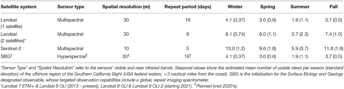
Table 1. Various current and planned satellites systems which are potentially useful for kelp aquaculture.

Canopy Analysis Using Landsat Imagery

Landsat 7 ETM+ imagery from June 30, 2019 was downloaded from the USGS Earth Explorer website (Table 2; earthexplorer.usgs.gov) as atmospherically corrected surface reflectance imagery. Kelp canopy fraction was determined following methods described in Cavanaugh et al. (2011) and Bell et al. (2020). Briefly, Landsat pixels were classified as containing kelp canopy using a binary decision tree using spectral bands 1–5, and 7. The fractional cover of kelp canopy inside each pixel was determined using Multiple Endmember Spectral Mixture Analysis (MESMA; Roberts et al., 1998), where the reflectance spectrum (spectral bands 1–4) of each pixel is iteratively modeled as a linear combination of one kelp canopy spectral endmember and one of 30 seawater endmembers. The 30 seawater endmembers were taken from Landsat pixels classified as seawater to account for varying spectral qualities due to sun glint, phytoplankton blooms, and suspended sediment. The optimal model, and resulting kelp canopy fraction estimate, minimizes the root mean squared error between the modeled and observed pixel reflectance spectrum. Kelp canopy fraction has been found to be linearly correlated with canopy biomass density using the empirical relationship between a time series of Landsat kelp canopy fraction estimates and monthly diver estimated canopy biomass at two permanent transects in the Santa Barbara Channel from 2003 to 2017 (Cavanaugh et al., 2011; Bell et al., 2020).

TABLE 2

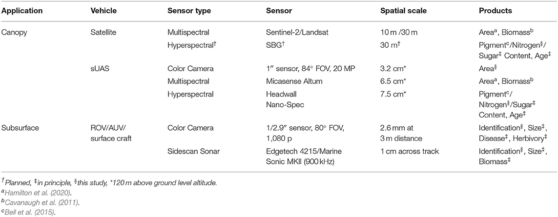
Table 2. Remote sensing technologies that can be used to monitor giant kelp aquaculture farms and the products which can be derived from the imagery.

Canopy Analysis Using sUAS Color Imagery

Aerial color digital imagery was obtained for the Arroyo Quemado kelp forest using a DJI Phantom 4 Pro sUAS, which is equipped with a 20 MP (1″ CMOS sensor, 84° FOV) color camera and can image areas of ~40 hectares in one flight (Table 2). All camera settings were set to automatic and there was no spectral calibration using calibration targets. Photogrammetric software (Agisoft Metashape Pro Version 1.5.0) was used to produce a georeferenced orthomosaic from the color imagery. Georeferencing was validated using known ground control points on land, approximately 200 m from the inshore edge of the kelp canopy. After land and breaking waves were removed from the color orthomosaic, floating kelp canopy was classified using a simple band ratio where Red is the red band and Blue is the blue band of the color image:

$\begin{array}{ll}KelpCanopy,\frac{Red}{Blue}\ge 1& (2)\end{array}$

$\begin{array}{ll}Seawater,\frac{Red}{Blue}<1& (3)\end{array}$

Canopy Analysis Using sUAS Multispectral Imagery

Multispectral aerial imagery was collected for the Arroyo Quemado kelp forest using the MicaSense Altum sensor mounted on a DJI Matrice 200 sUAS, which can also image areas of ~40 hectares in one flight (Table 2). The Altum sensor has five individual 3.2 MP cameras which simultaneously capture images across five spectral bands: blue (475 nm center, 32 nm bandwidth), green (560 nm center, 27 nm bandwidth), red (668 nm center, 14 nm bandwidth), red edge (717 nm center, 12 nm bandwidth), near infrared (840 nm center, 57 nm bandwidth). A 50% gray panel with a known reflectance across each of the five spectral bands was captured before and after the flight to convert each image to reflectance. Agisoft Metashape Pro software was used to produce a georeferenced orthomosaic for each spectral band (version 1.5.0). Kelp canopy density was determined using MESMA across all five spectral bands using one kelp spectral endmember and 10 seawater spectral endmembers (similar to the methods used with Landsat imagery in section Canopy Analysis Using Landsat Imagery). The kelp spectral endmember was determined using the mean spectrum of the 100 kelp canopy pixels with the highest near infrared reflectance (Supplementary Figure 1). Kelp canopy, like all photosynthetic material, displays a high reflectance in the near infrared, while seawater rapidly attenuates near infrared radiation (Cavanaugh et al., 2011; Bell et al., 2015). The 10 seawater endmembers were randomly chosen from seawater areas at least 50 m from the nearest kelp canopy (Supplementary Figure 1).

Canopy Analysis Using sUAS Hyperspectral Imagery

Hyperspectral aerial imagery was collected over the Arroyo Quemado kelp forest using a Headwall Nano-Hyperspec VNIR sensor mounted on a DJI Matrice 600 Pro sUAS, which can image areas of ~20 hectares in one flight (Table 2). The Nano-Hyperspec VNIR sensor measures a continuous reflectance spectrum from 400 to 1,000 nm across 270 contiguous 2.2 nm spectral bands. The sensor is a push broom scanner with 640 spatial bands and a 12 mm focal length lens, delivering a 7.2 cm pixel resolution at an altitude of 120 m. The sensor was calibrated before each flight by capturing a dark reference and a white reference using a 50% gray panel with a known spectral reflectance from 400 to 1,000 nm. A 3 × 3 m spectral reflectance calibration tarp comprised of three 3 × 1 m gray sections (11, 32, and 56% reflectance) was placed on the beach approximately 175 m inshore of the kelp canopy and was captured in the hyperspectral imagery. Image swaths were processed to surface reflectance data by first converting the recorded digital numbers to radiance using the dark reference and a sensor specific radiometric calibration file. Second, radiance was converted to surface reflectance using the three panels of the spectral reflectance calibration tarp captured in the imagery. The processed surface reflectance image swaths were individually orthorectified and georeferenced, and the positioning of each swath was then adjusted to match overlapping pixels between neighboring image swaths. All image processing was completed using the Headwall SpectralView software.

Each georeferenced image swath was then processed further using Matlab (version 2018b) first by smoothing all reflectance spectra using a Savitzky-Golay filter with a three-band window (Savitsky and Golay, 1964). Pixels containing glint were identified as all pixels where reflectance was >30% at the band centered at 731 nm and removed. Pixels were classified as kelp canopy where the ratio of reflectance at the band centered at 731 nm to the band centered at 509 nm was >3. Kelp canopy density was determined using MESMA across the entire reflectance spectrum using one kelp spectral endmember and 10 seawater spectral endmembers. The kelp spectral endmember was determined as the mean of the 100 kelp canopy pixels with the highest near infrared reflectance across all image swaths. The 10 seawater endmembers were randomly chosen from seawater areas at least 50 m from the nearest kelp canopy. After these additional processing steps, the resulting hyperspectral image was then georeferenced for a second time using the orthomosaic captured by the color camera sUAS to correct any spatial discrepancies.

Nitrogen Content Spectral Algorithm Development

In order to use spectral imagery to assess the condition of the kelp canopy using metrics such as tissue nitrogen content, empirical relationships must be developed between the spectra and the condition metric of interest. We used data of giant kelp blade reflectance with corresponding data of blade tissue nitrogen content collected monthly from 2012 to 2015 at three kelp forests in the Santa Barbara Channel to develop these relationships (see Bell et al., 2018 for detailed methods). Briefly, every month 15 mature canopy blades were collected at each of the three sites and their reflectance between 350 and 800 nm (1 nm intervals) was measured in the laboratory using a Shimadzu UV 2401PC spectrometer with an integrating sphere attachment. A 5 cm² disc was excised from the central portion of each blade and placed in a drying oven at 60°C for several days until completely dry. The dried discs were then combined, weighed, ground to a fine powder, and analyzed for nitrogen content using an elemental analyzer (Carlo-Erba Flash EA 1112 series, Thermo-Finnigan Italia, Milano, Italy). The mean reflectance spectra averaged over the 15 blades collected monthly for each site was paired with the pooled tissue nitrogen content of the 15 blades for the purpose of assessing the relationship between blade reflectance spectra and nitrogen content (n = 101 paired reflectance & nitrogen samples).

We focused on changes in the shape of the reflectance spectrum rather than the magnitude since sun glint or the proportion of kelp canopy inside an imaged pixel can have a large effect on reflectance magnitude (Cavanaugh et al., 2011). We first interpolated the 1 nm laboratory reflectance onto the 2.2 nm spectral bands associated with the Nano-Hyperspec sensor (full width at half maximum = 6.6 nm). Normalized reflectance (Nr) was determined by scaling reflectance (between 0 and 1) based on the maximum and minimum reflectance values of the spectral bands between 596 and 670 nm, an area of the spectrum important for diagnosing kelp physiological condition (Bell et al., 2015), and then adding a value of 1 to all spectral bands so that all values were positive. The bands in the range used for normalization represent wavelengths with low and relatively flat seawater reflectance and avoid the rapid increase in reflectance associated with the red edge of kelp canopy reflectance.

The ratio of Nr for all band pairs between 596 and 670 nm were iteratively compared to tissue nitrogen content across all 101 samples using linear and generalized additive models (GAMs; R package mgcv; Wood, 2017). Each GAM was fit between tissue nitrogen content and the predictor variable(s) with a Tweedie error structure (power function = 1.01; k = 5). In the visible light bands, differences in the spectral shape of reflectance are not a direct function of the tissue nitrogen content itself but are due to the additive absorption and fluorescence properties of various pigments (Gates et al., 1965; Woolley, 1971; Gausman, 1983; Hochberg et al., 2004). Photosynthetic pigment concentrations are modulated by both the ambient seawater nitrate concentration and available light, and different relationships may exist between pigment concentration and nitrogen content under nutrient vs. light limited conditions (Laws and Bannister, 1980). Due to these potential differences, photosynthetically active radiation (PAR) during the 30 days prior to sample collection was included as a predictor in the models. We compared model parsimony using the Akaike information criterion (AIC). Photosynthetically active radiation was determined using the closest 4 km daily MODIS Aqua product to each site (oceandata.sci.gsfc.nasa.gov; Bell et al., 2018).

Application of Nitrogen Algorithm to sUAS Hyperspectral Imagery

In order to create maps of kelp canopy nitrogen content, the tissue nitrogen content algorithm must be applied to the reflectance spectra measured by the Nano-Hyperspec VNIR. The hyperspectral image spectra were first normalized in the same manner as the laboratory reflectance spectra. Since each 7.2 cm pixel is a combination of kelp canopy and seawater, we used MESMA to estimate the fractional cover of kelp canopy and removed all pixels with a relative canopy fraction of <0.1 to minimize the effect of seawater on the reflectance spectra. Pixels with excessive noise were removed if the mean coefficient of variation of Nr between 565 and 610 nm (an area of the spectrum with low absorption by chlorophyll a) exceeded 10%. The nitrogen content spectral algorithm determined from the laboratory spectra was then applied to the hyperspectral imagery.

Subsurface Analysis Using Side Scan Sonar Imagery

Acoustic imagery of the aquaculture farm was captured using an Edgetech 4125 400/900 kHz side scan sonar system mounted 1 m below the water surface along the side of a 22-foot vessel moving at 3 km h⁻¹ (Table 2). The system's 900 kHz Compressed High-Intensity Radiated Pulse (CHIRP) pulse delivers an across track resolution of 1 cm and an onboard inertial measurement unit allows for correction of the imagery due to surface motion side scan imagery was collected on July 12 and July 30, 2019 along the length of one of the longlines of the Santa Barbara Mariculture giant kelp facility.

Subsurface Analysis Using Color Imagery

Underwater color imagery and video was captured by a high definition 1,080 p (1/2.9″ sensor, 80° FOV) color camera mounted on a Blue Robotics Remotely Operated Vehicle (ROV) on July 11 and July 29, 2019 along a portion of the same longline surveyed using side-scan sonar (Table 2). Visual analysis of the juvenile kelp growing on the longlines (number of pneumatocysts individual⁻¹) were performed for the portion of the longline surveyed on both dates using video collected by the ROV. The length of each kelp individual growing on the longline was measured by divers on July 12 and August 1, 2019. Elongation rate was determined for each individual kelp outplant that was measured on both dates by dividing the difference in maximum length by the number of days between surveys.

The images collected by the ROV were automatically analyzed for subsurface kelp outplant distribution using deep learning models trained from a set of human annotated imagery (ViQi, Inc.). The models used a Convolutional Neural Network (CNN; CaffeNet), which was pre-trained on the ImageNet dataset and used transfer learning techniques to train the models. Transfer learning was optimized to retrain the neural network while only fine-tuning the convolutional, feature retrieval, layers. This approach is especially useful when training with a small number of samples and when visual features created for natural image recognition are descriptive for the task in hand. Our training dataset consisted of five classes including ocean, kelp, longline, tag, and wire tie (plants were individually marked with tags affixed to the line with wire ties). Each class was manually annotated using polygonal outlines (405 ocean, 370 kelp, 316 long line, 338 tag, and 230 wire tie polygons). Since small numbers of training samples require additional methods to render good models, we exacted multiple samples from polygons using uniform gridding. The final training set consisted of >125,000 samples of ocean, >11,000 of kelp, >12,000 longline, >4,000 tags and >2,000 wire ties. The augmented dataset was then randomly partitioned into a training subset using 60% of the samples, withholding 20% for testing, and the final 20% for validation.

Results

Effect of Cloud Cover on the Usefulness of Satellite Observations

Cloud cover, which limits the ability of satellites to observe the ocean surface, displayed seasonal variability in the SCB over decadal time scales. Cloud cover over offshore areas was generally lowest in the winter ($\overline{x}=29.0\%$), increased in spring ($\overline{x}=47.2\%$) to a maximum in summer ($\overline{x}=67.5\%$) and declined in fall ($\overline{x}=35.4\%$). The seasonal pattern of cloud cover varied spatially (Figure 1), as cloud cover was fairly consistent in winter, spring, and fall (σ = 3.3, 5.0, and 4.3%, respectively), while offshore areas and windward coasts were generally cloudier than the leeward coasts of the mainland and islands during the summer (σ = 10.0%). The various satellite systems produced different numbers of usable images ranging from ~2 to 13 per season depending on their repeat time, number of satellites in a system, and seasonal cloud cover (Table 1).

FIGURE 1

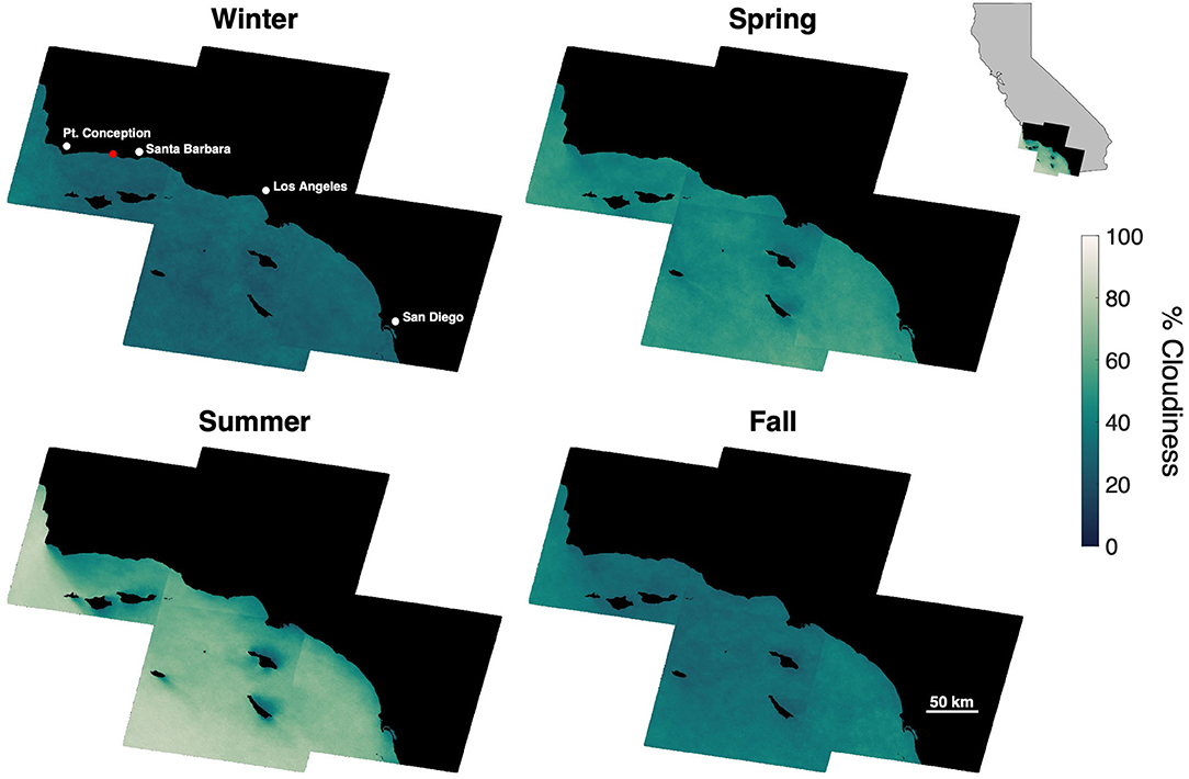
Figure 1. Mean seasonal cloud cover for areas offshore of Southern California at a 30 × 30 m pixel resolution, determined from 35 years of Landsat imagery (1984–2019). Red dot shows the location of the kelp forest in Figure 4.

Kelp Canopy Nitrogen Content Spectral Algorithm

Several spectral band ratios displayed strong linear and non-linear relationships with tissue nitrogen content. The ratio of Nr for any band located between 603 and 644 nm, and any band located between 665 and 680 nm was significantly and strongly linearly correlated with tissue nitrogen content. The changes in spectral shape in this region of the spectrum were superior for the estimation of tissue nitrogen content compared to spectral features in the blue, green, and near infrared wavelengths (Figure 2). The use of GAMs to incorporate the non-linearity of the relationship between the spectral band ratios and tissue nitrogen content led to the selection of the bands centered at 640 and 670 nm as the optimized wavelengths for the model:

$\begin{array}{ll}N{r}_{670nm}/N{r}_{640nm}& (4)\end{array}$

where Nr_670nm and Nr_640nm are the normalized reflectance at the bands centered at 670 and 640 nm, respectively (r² = 0.57; p < 0.0001; Figure 3A). Using both Nr_670nm/Nr_640nm and PAR as predictor variables (R² = 0.60; p < 0.0001, p = 0.015, respectively) decreased the AIC from 142.9 to 130.9, indicating a more parsimonious model. The effect of PAR on tissue nitrogen is demonstrated by the different relationships between Nr_670nm/Nr_640nm and tissue nitrogen content during high light (April–September) and low light (October–March) periods of the year (Figure 3A). The non-linear relationship between Nr_670nm/Nr_640nm and tissue nitrogen content displayed an effect size range of −0.48 to 0.68, and the relationship became positive at values >0.62 (Figure 3B). Photosynthetically active radiation displayed a linear relationship with tissue nitrogen content where the effect size of the relationship became positive at values >41 E m⁻² d⁻¹, with an effect size range of −0.11 to 0.09 (Figure 3C).

FIGURE 2

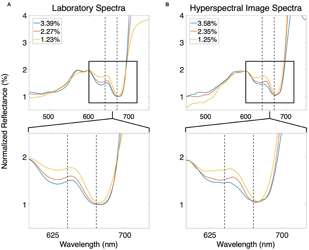
Figure 2. (A) Smoothed normalized reflectance spectra of giant kelp canopy blades with different tissue nitrogen contents measured in the laboratory. (B) Smoothed normalized reflectance spectra of the giant kelp canopy using the sUAS hyperspectral sensor. Tissue nitrogen content estimated using the ratio of the spectral bands centered at 670 and 640 nm (dashed black lines). The bottom panels show enlargements of the areas inside the black boxes in the top panels.

FIGURE 3

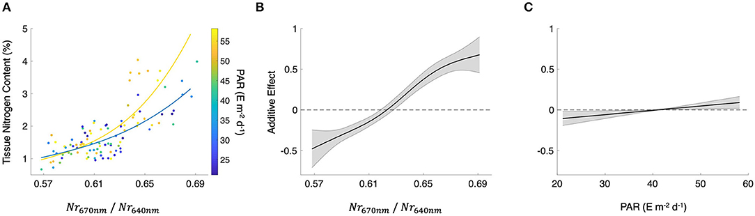
Figure 3. (A) Scatterplot of the spectral band ratio of normalized reflectance for bands centered at 670 and 640 nm (Nr_670nm/Nr_640nm) and tissue nitrogen content. Colored lines represent best fit lines between Nr_670nm/Nr_640nm and tissue nitrogen content in the high light season (yellow; April–September) and low light season (blue; October–March). Mean photosynthetically active radiation (PAR) for 30 days prior to the sampling date. (B) The additive effect of Nr_670nm/Nr_640nm on tissue nitrogen content and (C) the additive effect of PAR on tissue nitrogen content produced using a generalized additive model estimating tissue nitrogen content from both Nr_670nm/Nr_640nm and PAR. Black lines show the mean relationship and shaded gray areas show the standard error.

Assessment of Kelp Canopy Characteristics From Satellite and Aerial Imagery

In order to compare the various types of imagery and derived products, we surveyed a 10-hectare area containing kelp forest canopy with four different sensors over the course of a 3-h period. We first imaged the kelp canopy using the color camera on the Phantom 4 Pro sUAS, which produced a color orthomosaic with a final pixel resolution of 3.2 cm (Figure 4A). Kelp canopy and seawater were then classified from the color orthomosaic using (Equations 2 and 3) for a total estimated canopy area of 1.39 hectares (Figure 4B). The multispectral sensor onboard the Matrice 200 sUAS then imaged the study area, which produced an orthomosaic with a final pixel resolution of 6.5 cm. Kelp canopy fraction was then estimated using MESMA for the entire survey area ($\overline{x}=$ 0.059; σ= 0.174) and from all pixels containing kelp canopy (kelp canopy fraction >0; $\overline{x}=$ 0.424; σ= 0.250) for a total estimated canopy area of 1.41 hectares (Figure 4C). The hyperspectral sensor on the Matrice 600 Pro sUAS then imaged the study area to produce a map of canopy tissue nitrogen content ($\overline{x}=$ 2.32%; σ= 0.465%). The native 7.2 cm pixels were then interpolated onto a 25 cm grid, and all grid cells with less than three tissue nitrogen estimates were discarded (Figure 4D).

FIGURE 4

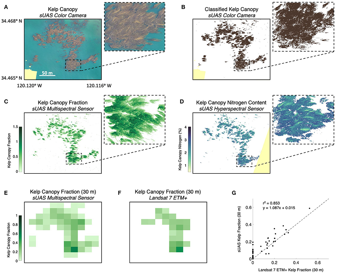
Figure 4. (A) Color orthomosaic of the Arroyo Quemado kelp forest canopy using the color camera on the Phantom 4 Pro sUAS (pixel resolution of 3.2 cm). (B) Kelp canopy classified from the color orthomosaic. (C) Fraction of each pixel covered by kelp canopy determined using Multiple Endmember Spectral Mixture Analysis (MESMA) with imagery from the sUAS multispectral sensor (pixel resolution of 6.5 cm). (D) Kelp canopy nitrogen content determined using the nitrogen content spectral algorithm with imagery from the sUAS hyperspectral sensor (pixel resolution 25 cm). (E) The mean kelp canopy fraction from the multispectral sensor binned into 30 m pixels to compare with (F). Kelp canopy fraction determined from the Landsat 7 ETM+ multispectral satellite sensor. (G) Comparison of the kelp canopy fraction from the multispectral sUAS sensor binned into 30 m pixels and the Landsat 7 ETM+ sensor. Pale yellow color shows areas not imaged by the sensor. All imagery acquired between 9:30 a.m. and 12 p.m. local time on June 30, 2019.

The Landsat 7 ETM+ satellite sensor imaged the survey area simultaneous to the sUAS flights and kelp canopy fraction was estimated from the entire survey area (Figure 4F; $\overline{x}=$ 0.037; σ= 0.088) and for all pixels classified as containing kelp canopy ($\overline{x}=$ 0.196; σ= 0.099). Kelp canopy fraction ranged from 0.074 to 0.523, corresponding to a 0.78–3.71 kg m⁻² range of canopy biomass density. Kelp canopy fractions from the multispectral sUAS imagery (6.5 cm) were interpolated to the 30 m Landsat grid and were compared using a linear regression (Figures 4E–G; r² = 0.853, p < 0.0001; y = 1.087 + 0.015). Overall, Landsat underestimated kelp canopy fractional cover by 33% when fractions were summed (6.71 vs. 4.50 summed kelp canopy fraction, respectively).

Acoustic Analysis of Juvenile Kelp Outplants on Farm Longlines

Kelp outplants increased in size between the two acoustic survey dates and diver measurements of the kelp outplants displayed an average elongation rate of 0.55 cm d⁻¹ (σ = 0.38; n = 50). Video analysis showed an increase in the number of pneumatocysts per outplant from 1.15 (σ = 1.87; n = 108) on July 11 to 6.18 (σ = 6.12; n = 97) on July 29, 2019 (Figure 5A). Side scan sonar imagery showed high acoustic returns for the longline and its structural buoys and weights during the survey on July 12, 2019. The subsequent side scan sonar survey on Jul 30, 2019 showed high acoustic returns for the same farm structures, as well as many objects attached to the top of the farm line (Figure 5B). These high acoustic returns were regularly spaced along the farm line and correspond to the general distance between the kelp outplants (~0.5 m).

FIGURE 5

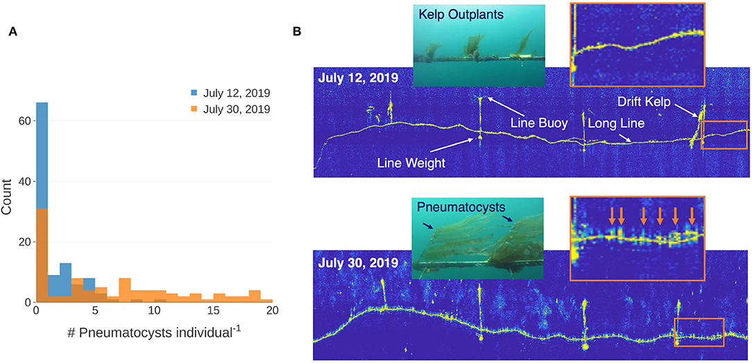
Figure 5. (A) Histogram showing the number of pneumatocysts per individual determined from video captured by a remotely operated vehicle (ROV) on a section of each line at each date. (B) Side scan sonar imagery of the line on July 12 and July 30, 2019 showing farm structures and a drifting kelp frond caught on the farm buoy. Insets inside the orange boxes show enlarged areas of sonar returns along the farm lines between the two dates. Orange arrows show high acoustics returns at the locations of probable kelp outplants. Color images captured by the ROV showing typical size of individual kelp outplants for each date.

Kelp Outplant Visualization Using Deep Learning Models

The resulting deep learning classification model, which included all five object classes, detected kelp with 72% accuracy (percent of kelp class polygons correctly identified) and 32% error (percent of non-kelp class polygons incorrectly identified as kelp). After initial validation, we refined the model by disabling poorly performing classes (accuracy <25%). Since our primary objective was to detect kelp outplants, we also disabled classes deemed unnecessary (background ocean and wire tie). Disabling the ocean and wire tie classes reduced errors introduced to other classes and positively affected model performance, with the final model detecting kelp with 91% accuracy and 7% error, while longline detection demonstrated 68% accuracy and 2% error. The model produced polygonal annotations of kelp and longline classes that visually resembled human annotations (Figure 6).

FIGURE 6

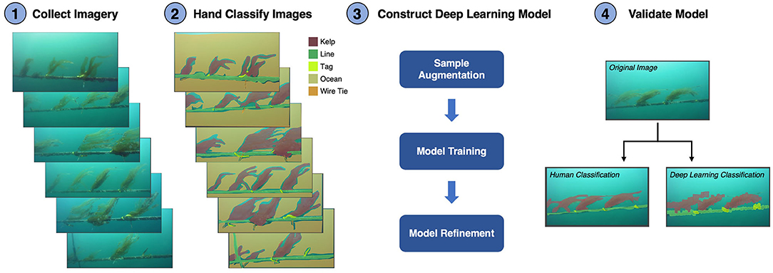
Figure 6. Schematic showing the steps to develop and validate the deep learning model used to automatically classify giant kelp juveniles on an aquaculture farm. (1) Collect imagery of the farm lines using a color camera mounted on an underwater vehicle. (2) The images (n = 137) were classified by hand into five classes: Kelp, Line, Tag, Ocean, and Wire Tie. Light blue areas show sections of the background ocean which were not classified by hand. (3) The number of samples for model training was augmented by extracting multiple samples from inside the polygons of each class. The model was then trained using 60% of the images with a convolutional neural network and refined using 20% of the images. Model refinement involves identifying and removing poorly performing classes. (4) The final model was validated using the final 20% of the imagery by comparing hand classifications to the deep learning classifications.

Discussion

Remote Monitoring of the Kelp Canopy

Aerial and spaceborne imaging of the floating kelp canopy have the potential to deliver several actionable products to offshore aquaculture managers (Table 2 and Figure 4). Satellite observations of the kelp canopy represent the most mature sector of the aquaculture monitoring platforms examined in this study as these sensors have been used to assess natural kelp forest dynamics over 100's of km (Cavanaugh et al., 2019). The spectral and spatial resolution (30 m) of the Landsat satellite sensors can provide estimates of canopy biomass that compare well to over a decade of in situ diver estimates (Bell et al., 2020). However, because existing operational multispectral satellites were primarily designed for terrestrial targets (Table 1), only the area or biomass of canopy forming kelp species can be determined. The mixture of kelp canopy and seawater in each 10–30 m pixel limits their ability to use common multispectral band ratios to estimate plant physiological condition or the elemental content of the tissue (Table 2; Cavanaugh et al., 2010, Cavanaugh et al., 2011; Bell et al., 2015). In the near future, opportunities exist for more comprehensive spaceborne monitoring of kelp aquaculture farms using global, repeat hyperspectral imaging. The Surface Biology and Geology (SBG) designated observable (a set of targeted observation capabilities from a future spaceborne mission) will provide the spectral coverage and resolution necessary to estimate the physiology and macromolecular content of the kelp canopy in the presence of seawater (Bell et al., 2015; Lee et al., 2015). For example, the spectral bands centered at 640 and 670 nm will be measured by the proposed satellite sensor and can assess the physiological condition and nitrogen content of the kelp canopy without relying on bands in the red edge (680–750 nm) and near infrared (>750 nm) regions, which are rapidly attenuated by seawater (Mobley, 1994).

The temporal resolution of satellite imagery and the lack of flexibility in image acquisition timing restrict the monitoring capabilities of satellite imagery for offshore aquaculture. Publicly available imagery (Table 1) are acquired on a 5 to 16 day repeat cycle regardless of cloud cover. Cloud cover in offshore areas of the Southern California Bight is considerably higher than coastal areas especially in the summer (Figure 1), a period when frequent monitoring may be vital to optimize production and harvest timing. However, by combining the imagery of multiple satellite systems there is an enhanced opportunity of a cloud-free view in any season (Li and Roy, 2017). Additionally, spatial resolution may also be problematic since pixel resolution is typically between 10 and 30 m (Table 2). Fine scale canopy features will likely be lost as the reflectance signal is averaged over larger areas, which may include floating farm structures (Figures 4E–G; Cui et al., 2019). Higher resolution satellite imagery (0.5–3 m) can be expensive to acquire, not publicly available, and/or not feasible for repeat imaging on the time scales necessary to deliver actionable information (Fan et al., 2018; Fu et al., 2019; Zhu et al., 2019). Despite the increased cloud cover in the offshore zone, moderate spatial resolution satellite sensors (daily repeat interval, more consistent coverage) could be used to monitor the farm environment (e.g., sea surface temperature). While these sensors cannot provide direct observations of the kelp canopy, valuable products such as seawater nitrate concentration can be empirically derived from satellite determinations of sea surface temperature (Kamykowski and Zentara, 1986; Snyder et al., 2020).

While there has been an increased use of sUAS for agricultural crop monitoring over the past decade (reviewed in Puri et al., 2017), their use in aquaculture has been rare (Reshma and Kumar, 2016). Despite their paucity of use, quality imagery of the kelp canopy can be acquired with a variety of sUAS mounted sensors, delivering maps of canopy area, canopy biomass, and physiological metrics such as tissue nitrogen content (Figures 4A–D). Commercially available color and multispectral sensors can rapidly capture imagery over ~40 hectares in a single flight, and canopy area can be classified without the need for sophisticated analysis or expensive sensors (Figure 4B). The considerable differences in reflectance between seawater and the floating kelp canopy allows for a simple band ratio of the red and blue spectral bands to differentiate the classes. Furthermore, the high spatial resolution (~5 cm) of this imagery can quantify sparse canopy which may be missed by the lower resolution imagery acquired by satellite sensors (Figures 4E–G). Hyperspectral sensors can provide the spectral data necessary to estimate the physiological and tissue content metrics of the kelp canopy through the quantification of photosynthetic pigment concentrations (Figure 4D; Bell et al., 2015; Adão et al., 2017). The chlorophyll a pigment absorbs blue and red wavelengths to drive the photosynthetic process, with absorption peaks at 430 nm and 662 nm. Giant kelp lacks the chlorophyll b pigment (absorption peaks at 453 and 642 nm) but possesses the chlorophyll c pigment (absorption peaks at 444 and 626 nm; Wheeler, 1980). The absence of the chlorophyll b pigment produces a peak in the kelp reflectance spectrum at ~640 nm and provides a reference point to assess the relative spectral absorption associated with the chlorophyll a pigment at ~670 nm (Figure 2). While the spectral information at 640 and 670 nm can be used to assess the concentration of the chlorophyll a pigment (Bell et al., 2015), the relationship between pigment concentration and tissue nitrogen content is also a function of the amount of sunlight reaching the surface canopy (Figure 4). Marine photosynthetic organisms optimize pigment concentrations in response to available light through photoacclimation, where increased solar irradiance lessens the need for high pigment concentrations to maximize photosynthesis (Laws and Bannister, 1980). While an increase in photosynthetic pigment is positively associated with a higher tissue nitrogen content, this relationship is modulated by light (Figure 3), and these functions can be applied to spectral imagery to generate maps of tissue nitrogen content across large areas of kelp canopy (Figure 4D). Knowledge of the spatial patterns of physiological condition and tissue content metrics of the kelp canopy can be used to map farm production and time harvest to maximize desired biomass quality (i.e., nitrogen content). However, the sheer volume of data collected by hyperspectral sensors is immense, spectra are difficult to process, and pre-flight calibration procedures make these sensors challenging to use in an operational capacity. Research using hyperspectral imaging to identify the specific spectral bands necessary for the simultaneous estimation of valuable canopy traits (e.g., biomass, nitrogen/sugar content, age) could lead to user-friendly multispectral sensors with specific bands tailored for kelp canopy monitoring (Figure 2).

Remote Quantification of Subsurface Kelp Outplants

Since juvenile kelp stages are especially sensitive to changing environmental conditions, competition, and herbivory, it may be important to assess the state of kelp outplants prior to canopy development using subsurface sensors (Dean et al., 1984; Hernández-Carmona et al., 2001; Gorman and Connell, 2009). The automated analysis of underwater color imagery using deep learning models could enable repeat monitoring of kelp juveniles on offshore farms. Machine learning based methods have already been successfully applied to underwater color imagery to classify fish species and quantify the biodiversity of marine sessile communities (Rahimi et al., 2014; Salman et al., 2016). In this study, a small set of underwater imagery collected by an inexpensive color camera mounted on an ROV was used to train a deep learning model and successfully classify kelp, tags, and longlines despite changes in kelp orientation due to water motion (Figure 6). These methods have advantages over spectral analyses as depth, bottom reflectance, and standoff distance of the sensor can significantly change the measured reflectance spectrum (Mobley, 1994). These tools should also be adaptable to other kelp aquaculture monitoring tasks such as quantifying epibiont load or identifying the presence of herbivores. Capturing usable underwater color imagery requires clear water and sufficient solar illumination to produce satisfactory results. Fortunately, suspended particle concentrations are reduced in the offshore environments off the Southern California coast which should lead to greater opportunities for underwater image collection (Henderikx Freitas et al., 2017). Additionally, offshore farm structures can be equipped with inexpensive turbidity or light sensors in order to optimize the timing of image acquisition.

Acoustic measurements do not require light and are also less sensitive to water clarity than optical imaging and high-quality measurements can be acquired at any time of day and across a range of seawater conditions (Gonzalez-Socoloske et al., 2009). Side scan sonar is particularly useful to identify kelp outplants once the juveniles produce gas filled pneumatocysts, which lead to enhanced acoustic returns (Figure 5; Wilson, 2011). Since a pneumatocyst exists at the base of each giant kelp blade, there is a strong linear relationship between total gas volume and kelp biomass, such that acoustic imagery is ideal for monitoring the spatial arrangement and growth of subsurface stages of giant kelp on aquaculture farms (Wilson, 2011). Future development of these technologies also brings new opportunities, as many farmed kelp species never produce a floating canopy and require subsurface monitoring using acoustic sensors or color imaging (Fischell et al., 2019). These techniques could be deployed to survey numerous species and have potential for monitoring across aquaculture industries.

Operational Risks and Limitations

While the use of remote sensing platforms for offshore aquaculture monitoring reduces risks and costs related to in situ monitoring there are several limitations to these platforms that must be addressed before they are used in an operational context (Table 3). At the present time, monitoring with satellite platforms presents the fewest operational limitations. Sensor hardware failures are rare, though they may occasionally lead to missing data or failure of the sensor system (Markham et al., 2004; Chan et al., 2018). While the advent of freely available imagery has led to massive increases in both research and commercial remote sensing applications, there is no guarantee that these policies will exist in perpetuity (Zhu, 2019).

TABLE 3

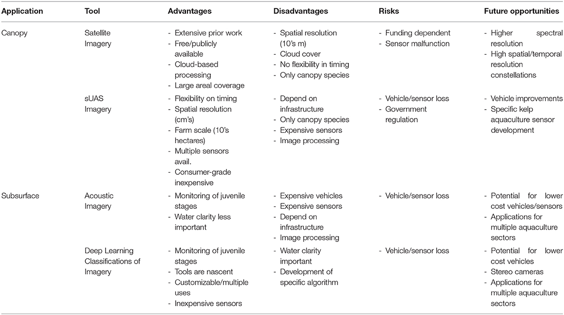
Table 3. The advantages, disadvantages, risks, and future opportunities of various remote sensing technologies applicable to offshore kelp aquaculture farms.

A major limiting factor for sUAS monitoring of offshore kelp aquaculture farms is the lack of available docking, charging, and data downlink infrastructure necessary for the autonomous and repeat deployment of these systems. However, there are several recent patents outlining the design of these systems, suggesting that such capabilities may be available in the near future (Garrec and Cornic, 2012; Yu et al., 2016; Gentry et al., 2018). While consumer grade sUAS equipped with color cameras are relatively inexpensive (< $1,500 USD), multispectral sensors can cost several thousand dollars. Processing of the individual images (e.g., orthorectification, mosaicking) is the responsibility of the user and precise georeferencing and radiometric calibration must be performed before mosaics and their derived products can be compared (Cruzan et al., 2016; Doughty and Cavanaugh, 2019). These tasks have been greatly simplified for users without image analysis training by several companies who offer cloud-based image processing through subscription services. Any autonomous vehicle carries a risk of loss associated with mechanical failure, GPS signal interference, and an inability to react to novel situations (Milanés et al., 2008). Additionally, while the U.S. Federal Aviation Administration adopted regulations allowing for extensive agricultural monitoring activities by sUAS in 2016, current regulations only allow for ‘line of sight’ operation where the pilot must maintain visual observation of the vehicle (Patel, 2016). Such rules will need to be adjusted for the sUAS monitoring of offshore aquaculture to become a reality.

While autonomous underwater vehicles are a promising monitoring platform for both acoustic and color imaging, there are both significant cost and operational risk barriers that must be crossed before these systems become viable monitoring options. Research-grade side scan sonar systems cost tens of thousands of dollars, although there has been recent success in monitoring submerged aquatic vegetation with less expensive consumer-grade systems (Greene et al., 2018). While the cost of autonomous underwater vehicles is currently prohibitive to most aquaculture operations, several small and low-cost vehicles are entering the market space and may revolutionize the collection of acoustic and color imagery in the coming years, and the development cost-effective infrastructure for docking, charging, and data downlink for these vehicles is an active area of research (Hobson et al., 2003; Pyle et al., 2012; Manley and Smith, 2017). Due to these high costs, the loss of underwater vehicles and their associated sensors a paramount concern. New statistical approaches to inform the probability of vehicle loss could be used to determine low risk conditions and provide adaptive mission management for these autonomous platforms (Brito and Griffiths, 2016).

Additionally, it is important to assess the risks these monitoring platforms and large-scale offshore aquaculture farms present to the environment. While sUAS carry limited risk to the environment outside of vehicle loss, their potential effects on the behavior of seabirds is an often-cited concern. Studies have found minimal negative effects of sUAS while censusing nesting colonies (Brisson-Curadeau et al., 2017) however aquaculture operations should be situated away from wildlife areas to avoid potential interactions. Below water, the acoustic imaging systems examined in this study (side scan sonar) generate high-frequency sound at the upper limit of the audible spectrum and are unlikely to cause a behavioral response from marine mammals (MacGillivray et al., 2013). Potential negative impacts of large-scale offshore aquaculture structures including wildlife interactions, shipping hazards, and the generation of marine debris are valid concerns and robust spatial planning should be prioritized to reduce conflicts and avoid environmental impacts (Gentry et al., 2017b; Lester et al., 2018).

Conclusions

This examination of remote sensing technologies guides the best uses of these platforms to deliver actionable products for offshore kelp aquaculture farms. Kelp outplant viability and growth are most readily assessed using underwater color imagery classified with deep learning models. This combination of inexpensive cameras and machine learning leads to the rapid identification and sizing of small juvenile kelps, measuring survivorship and growth much earlier than other subsurface monitoring technologies. The use of deep learning models to detect kelp in color imagery could be enhanced by future research developing additional models that quantify the abundance of kelp herbivores and epibionts. Acoustic imaging from side scan sonar is most effective once pneumatocysts have developed and used to track the growth of subsurface kelp fronds that are too large to be imaged using color imagery (Wilson, 2011). While the monitoring of kelp farms with underwater side scan sonar and color imaging shows great promise, their implementation relies on the development of low-cost AUVs and docking infrastructure (Hobson et al., 2003; Pyle et al., 2012; Manley and Smith, 2017). Additional research using consumer-grade side scan sonar sensors to quantify subsurface kelp will also reduce costs (Greene et al., 2018). Due to high summertime cloud cover in offshore areas, satellite imagery is most useful for large-scale monitoring of the farm environment using daily, moderate spatial resolution estimates of sea surface temperature and derived products such as seawater nitrate concentration (Snyder et al., 2020). Due to the rapid growth, turnover, and senescence rates of giant kelp, observations of kelp canopy biomass quantity and condition, such as tissue nitrogen content, are most readily achieved using sUAS imagery (Clendenning, 1971; Rodriguez et al., 2013; Rassweiler et al., 2018). Improvements in sUAS infrastructure, multispectral sensors customized for estimating kelp canopy traits, and a relaxation of the ‘line of sight’ regulation for offshore areas will strengthen the role of kelp canopy monitoring by sUAS.

Data Availability Statement

The datasets generated for this study are available on request to the corresponding author.

Author Contributions

TB, RM, NNi, and DS conceived the study and wrote the manuscript. TB, JS, and MG processed satellite imagery for the cloud cover analysis. TB, JS, and CM collected and processed the sUAS imagery of kelp canopy. DS, TB, KyC, and KaC developed the color and multispectral sUAS algorithms. TB, JS, NNe, and DR collected the laboratory spectral measurements and performed the pigment and elemental analyses. TB, NNe, and MG developed the tissue nitrogen content spectral algorithm. NNi and CM collected and processed the underwater color and acoustic imagery of the kelp outplants. DF and CM developed the deep learning algorithms. DR, RM, and CY collected and processed the in situ data of the kelp outplants. All authors contributed to interpreting the results and revising the manuscript.

Funding

This was supported by the US Department of Energy's Advanced Research Projects Agency–Energy (ARPA-E; DE-AR0000922 and DE-AR0000914), the US National Science Foundation (OCE 1831937), and by the National Aeronautics and Space Administration (NNX14AR62A).

Conflict of Interest

DF was employed by the company ViQi, Inc.

The remaining authors declare that the research was conducted in the absence of any commercial or financial relationships that could be construed as a potential conflict of interest.

Acknowledgments

We would like to thank all individuals involved with the UCSB/USC/UWM ARPA-E MARINER kelp genetics project who outplanted and maintained the kelp farm off the coast of Santa Barbara. We would also like to extend a sincere thanks to the many field technicians and student volunteers who conduct field and laboratory work for the Santa Barbara Coastal LTER. Special thanks go to guest editors Dr. Stephanie Palmer, Dr. Pierre Gernez, Dr. Rodney Forster, and Dr. Yoann Thomas.

Supplementary Material

The Supplementary Material for this article can be found online at: https://www.frontiersin.org/articles/10.3389/fmars.2020.520223/full#supplementary-material

References

Ackleson, S. G., Smith, J. P., Rodriguez, L. M., Moses, W. J., and Russell, B. J. (2017). Autonomous coral reef survey in support of remote sensing. Front. Mar. Sci. 4:325. doi: 10.3389/fmars.2017.00325

CrossRef Full Text | Google Scholar

Adão, T., Hruška, J., Pádua, L., Bessa, J., Peres, E., Morais, R., et al. (2017). Hyperspectral imaging: a review on uav-based sensors, data processing and applications for agriculture and forestry. Remote Sens. 9:1110. doi: 10.3390/rs9111110

CrossRef Full Text | Google Scholar

Bell, T. W., Allen, J. G., Cavanaugh, K. C., and Siegel, D. A. (2020). Three decades of variability in California's giant kelp forests from the Landsat satellites. Remote Sens. Environ. 238:110811. doi: 10.1016/j.rse.2018.06.039

CrossRef Full Text | Google Scholar

Bell, T. W., Cavanaugh, K. C., and Siegel, D. A. (2015). Remote monitoring of giant kelp biomass and physiological condition: an evaluation of the potential for the Hyperspectral Infrared Imager (HyspIRI) mission. Remote Sens. Environ. 167, 218–228. doi: 10.1016/j.rse.2015.05.003

CrossRef Full Text | Google Scholar

Bell, T. W., Reed, D. C., Nelson, N. B., and Siegel, D. A. (2018). Regional patterns of physiological condition determine giant kelp net primary production dynamics. Limnol. Oceanogr. 63, 472–483. doi: 10.1002/lno.10753

CrossRef Full Text | Google Scholar

Brisson-Curadeau, É., Bird, D., Burke, C., Fifield, D. A., Pace, P., Sherley, R. B., et al. (2017). Seabird species vary in behavioural response to drone census. Sci. Rep. 7:17884. doi: 10.1038/s41598-017-18202-3

PubMed Abstract | CrossRef Full Text | Google Scholar

Brito, M., and Griffiths, G. (2016). A Bayesian approach for predicting risk of autonomous underwater vehicle loss during their missions. Reliab. Eng. Syst. Saf. 146, 55–67. doi: 10.1016/j.ress.2015.10.004

CrossRef Full Text | Google Scholar

Card, D. H., Peterson, D. L., Matson, P. A., and Aber, J. D. (1988). Prediction of leaf chemistry by the use of visible and near infrared reflectance spectroscopy. Remote Sens. Environ. 26, 123–147. doi: 10.1016/0034-4257(88)90092-2

CrossRef Full Text | Google Scholar

Cavanaugh, K., Siegel, D., Kinlan, B., and Reed, D. (2010). Scaling giant kelp field measurements to regional scales using satellite observations. Mar. Ecol. Prog. Ser. 403, 13–27. doi: 10.3354/meps08467

CrossRef Full Text | Google Scholar

Cavanaugh, K., Siegel, D., Reed, D., and Dennison, P. (2011). Environmental controls of giant kelp biomass in the Santa Barbara Channel, California. Mar. Ecol. Prog. Ser. 429, 1–17. doi: 10.3354/meps09141

CrossRef Full Text | Google Scholar

Cavanaugh, K. C., Reed, D. C., Bell, T. W., Castorani, M. C. N., and Beas-Luna, R. (2019). Spatial variability in the resistance and resilience of giant kelp in southern and Baja California to a multiyear heatwave. Front. Mar. Sci. 6:413. doi: 10.3389/fmars.2019.00413

CrossRef Full Text | Google Scholar

Chan, S. K., Bindlish, R., O'Neill, P., Jackson, T., Njoku, E., Dunbar, S., et al. (2018). Development and assessment of the SMAP enhanced passive soil moisture product. Remote Sens. Environ. 204, 931–941. doi: 10.1016/j.rse.2017.08.025

PubMed Abstract | CrossRef Full Text | Google Scholar

Clendenning, K. A. (1971). “Photosynthesis and general development,” in The Biology of Giant Kelp Beds (Macrocystis) in California. Beihefte Zur Nova Hedwigia. Lehre, ed W. J. North (Coley: Verlag Von J. Cramer), 169–190.

Google Scholar

Correa, T., Gutiérrez, A., Flores, R., Buschmann, A. H., Cornejo, P., and Bucarey, C. (2016). Production and economic assessment of giant kelp Macrocystis pyrifera cultivation for abalone feed in the south of Chile. Aquac. Res. 47, 698–707. doi: 10.1111/are.12529

CrossRef Full Text | Google Scholar

Cruzan, M. B., Weinstein, B. G., Grasty, M. R., Kohrn, B. F., Hendrickson, E. C., Arredondo, T. M., et al. (2016). Small unmanned aerial vehicles (micro-uavs, drones) in plant ecology. Appl. Plant Sci. 4:1600041. doi: 10.3732/apps.1600041

CrossRef Full Text | Google Scholar

Cui, B., Fei, D., Shao, G., Lu, Y., and Chu, J. (2019). Extracting raft aquaculture areas from remote sensing images via an improved U-Net with a PSE structure. Remote Sens. 11:2053. doi: 10.3390/rs11172053

CrossRef Full Text | Google Scholar

Dean, T. A., Schroeter, S. C., and Dixon, J. D. (1984). Effects of grazing by two species of sea urchins (Strongylocentrotus franciscanus and Lytechinus anamesus) on recruitment and survival of two species of kelp (Macrocystis pyrifera and Pterygophora californica). Mar. Biol. 78, 301–313. doi: 10.1007/BF00393016

CrossRef Full Text | Google Scholar

Doughty, C., and Cavanaugh, K. (2019). Mapping coastal wetland biomass from high resolution unmanned aerial vehicle (UAV) imagery. Remote Sens. 11:540. doi: 10.3390/rs11050540

CrossRef Full Text | Google Scholar

Drusch, M., Del Bello, U., Carlier, S., Colin, O., Fernandez, V., Gascon, F., et al. (2012). Sentinel-2: ESA's Optical High-Resolution Mission for GMES Operational Services. Remote Sens. Environ. 120, 25–36. doi: 10.1016/j.rse.2011.11.026

CrossRef Full Text | Google Scholar

Fan, J., Zhao, J., Song, D., Wang, X., Wang, X., and Su, X. (2018). Marine floating raft aquaculture dynamic monitoring based on multi-source GF Imagery. in 2018 7th International Conference on Agro-geoinformatics (Agro-geoinformatics) (Hangzhou: IEEE), 1–4. doi: 10.1109/Agro-Geoinformatics.2018.8476085

CrossRef Full Text | Google Scholar

Fedorov, D. V., Kvilekval, Kristian, G., Doheny, B., Sampson, S., Miller, R. J., and Manjunath, B. S. (2017). Deep Learning for All: Managing and Analyzing Underwater and Remote Sensing Imagery on the Web Using BisQue. UC Santa Barbara. Retrieved from: https://escholarship.org/uc/item/9z73t7hv (accessed November 29, 2020).

Google Scholar

Fischell, E. M., Gomez-ibanez, D., Lavery, A., Stanton, T., and Kukulya, A. (2019). “Autonomous underwater vehicle perception of infrastructure and growth for aquaculture,” in IEEE ICRA Workshop, Underwater Robotic Perception 2019 (Montreal, QC), 1–7

Fu, Y., Ye, Z., Deng, J., Zheng, X., Huang, Y., Yang, W., et al. (2019). Finer resolution mapping of marine aquaculture areas using worldview-2 imagery and a hierarchical cascade convolutional neural network. Remote Sens. 11:1678. doi: 10.3390/rs11141678

CrossRef Full Text | Google Scholar

Garrec, P., and Cornic, P. (2012). Autonomous and Automatic Landing System for Drones. U.S. Patent No. 8,265,808 B2. Washington, DC: U.S. Patent and Trademark Office.

Google Scholar

Gates, D. M., Keegan, H. J., Schleter, J. C., and Weidner, V. R. (1965). Spectral properties of plants. Appl. Opt. 4:11. doi: 10.1364/AO.4.000011

CrossRef Full Text | Google Scholar

Gausman, H. W. (1983). Visible light reflectance, transmittance, and absorptance of differently pigmented cotton leaves. Remote Sens. Environ. 13, 233–238. doi: 10.1016/0034-4257(83)90041-X

CrossRef Full Text | Google Scholar

Gentry, N., Hsieh, R., and Nguyen, L. (2018). Multi-Use UAV Docking Station Systems and Methods. U.S. Patent No. 9,387,928 B1. Washington, DC: U.S. Patent and Trademark Office.

Google Scholar

Gentry, R. R., Froehlich, H. E., Grimm, D., Kareiva, P., Parke, M., Rust, M., et al. (2017a). Mapping the global potential for marine aquaculture. Nat. Ecol. Evol. 1, 1317–1324. doi: 10.1038/s41559-017-0257-9

PubMed Abstract | CrossRef Full Text | Google Scholar

Gentry, R. R., Lester, S. E., Kappel, C. V., White, C., Bell, T. W., Stevens, J., et al. (2017b). Offshore aquaculture: spatial planning principles for sustainable development. Ecol. Evol. 7:2637. doi: 10.1002/ece3.2637

PubMed Abstract | CrossRef Full Text

Gonzalez-Socoloske, D., Olivera-Gomez, L. D., and Ford, R. E. (2009). Detection of free-ranging West Indian manatees Trichechus manatus using side-scan sonar. Endanger. Species Res. 8, 249–257. doi: 10.3354/esr00232

CrossRef Full Text | Google Scholar

Gorelick, N., Hancher, M., Dixon, M., Ilyushchenko, S., Thau, D., and Moore, R. (2017). Google earth engine: planetary-scale geospatial analysis for everyone. Remote Sens. Environ. 202, 18–27. doi: 10.1016/j.rse.2017.06.031

CrossRef Full Text | Google Scholar

Gorman, D., and Connell, S. D. (2009). Recovering subtidal forests in human-dominated landscapes. J. Appl. Ecol. 46, 1258–1265. doi: 10.1111/j.1365-2664.2009.01711.x

CrossRef Full Text | Google Scholar

Graham, M. H., Vasquez, J. A., and Buschmann, A. H. (2007). Global ecology of the giant kelp Macrocystis: from ecotypes to ecosystems. Oceanogr. Mar. Biol. An Annu. Rev. 45, 39–88. doi: 10.1201/9781420050943.ch2

CrossRef Full Text | Google Scholar

Greene, A., Rahman, A. F., Kline, R., and Rahman, M. S. (2018). Side scan sonar: A cost-efficient alternative method for measuring seagrass cover in shallow environments. Estuar. Coast. Shelf Sci. 207, 250–258. doi: 10.1016/j.ecss.2018.04.017

CrossRef Full Text | Google Scholar

Gutierrez, A., Correa, T., Muñoz, V., Santibañez, A., Marcos, R., Cáceres, C., et al. (2006). Farming of the giant kelp Macrocystis pyrifera in southern chile for development of novel food products. J. Appl. Phycol. 18, 259–267. doi: 10.1007/s10811-006-9025-y

CrossRef Full Text | Google Scholar

Hamilton, S. L., Bell, T. W., Watson, J. R., Grorud-Colvert, K. A., and Menge, B. A. (2020). Remote sensing: generation of long-term kelp bed data sets for evaluation of impacts of climatic variation. Ecology 101:e03031. doi: 10.1002/ecy.3031

PubMed Abstract | CrossRef Full Text | Google Scholar

Hardin, P. J., Lulla, V., Jensen, R. R., and Jensen, J. R. (2019). Small Unmanned Aerial Systems (sUAS) for environmental remote sensing: challenges and opportunities revisited. GIScience Remote Sens. 56, 309–322. doi: 10.1080/15481603.2018.1510088

CrossRef Full Text | Google Scholar

Henderikx Freitas, F., Siegel, D. A., Maritorena, S., and Fields, E. (2017). Satellite assessment of particulate matter and phytoplankton variations in the Santa Barbara Channel and its surrounding waters: role of surface waves. J. Geophys. Res. Ocean. 122, 355–371. doi: 10.1002/2016JC012152

CrossRef Full Text | Google Scholar

Hernández-Carmona, G., Robledo, D., and Serviere-Zaragoza, E. (2001). Effect of nutrient availability on Macrocystis pyrifera recruitment and survival near its southern limit off Baja California. Bot. Mar. 44, 221–229. doi: 10.1515/BOT.2001.029

CrossRef Full Text | Google Scholar

Hobson, B., Schulz, B., Pinnix, H., and Moody, R. (2003). Low-Cost UUVs for Task Specific and Expendable Missions. Technol. [C/CD], 2–5. Available online at: https://www.researchgate.net/publication/228902666_Low-cost_UUVs_for_task_specific_and_expendable_missions (accessed November 29, 2020).

Google Scholar

Hochberg, E. J., Atkinson, M. J., Apprill, A., and Andréfouët, S. (2004). Spectral reflectance of coral. Coral Reefs 23, 84–95. doi: 10.1007/s00338-003-0350-1

CrossRef Full Text | Google Scholar

Kamykowski, D., and Zentara, S.-J. (1986). Predicting plant nutrient concentrations from temperature and sigma-t in the upper kilometer of the world ocean. Deep Sea Res. Part A Oceanogr. Res. Pap. 33, 89–105. doi: 10.1016/0198-0149(86)90109-3

CrossRef Full Text | Google Scholar

Laws, E., and Bannister, T. (1980). Nutrient and light-limited growth of Thalassiosira fluviatilis in continuous culture, with implications for phytoplankton growth in the ocean. Limnol. Oceanogr. 25, 457–473. doi: 10.4319/lo.1980.25.3.0457

CrossRef Full Text | Google Scholar

Lee, C. M., Cable, M. L., Hook, S. J., Green, R. O., Ustin, S. L., Mandl, D. J., et al. (2015). An introduction to the NASA hyperspectral InfraRed imager (HyspIRI) mission and preparatory activities. Remote Sens. Environ. 167, 6–19. doi: 10.1016/j.rse.2015.06.012

CrossRef Full Text | Google Scholar

Lester, S. E., Stevens, J. M., Gentry, R. R., Kappel, C. V., Bell, T. W., Costello, C. J., et al. (2018). Marine spatial planning makes room for offshore aquaculture in crowded coastal waters. Nat. Commun. 9:945. doi: 10.1038/s41467-018-03249-1

PubMed Abstract | CrossRef Full Text | Google Scholar

Li, J., and Roy, D. P. (2017). A global analysis of sentinel-2A, sentinel-2B and landsat-8 data revisit intervals and implications for terrestrial monitoring. Remote Sens. 9:902. doi: 10.3390/rs9090902

CrossRef Full Text | Google Scholar

Lovatelli, A., Aguilar-Manjarrez, J., and Soto, D. (2013). Expanding mariculture farther offshore: Technical, environmental, spatial and governance challenges. FAO Technical Workshop (p. 73). Orbetello: FAO Fisheries and Aquaculture Department.

Google Scholar

Lund-Hansen, L. C., Juul, T., Eskildsen, T. D., Hawes, I., Sorrell, B., Melvad, C., et al. (2018). A low-cost remotely operated vehicle (ROV) with an optical positioning system for under-ice measurements and sampling. Cold Reg. Sci. Technol. 151, 148–155. doi: 10.1016/j.coldregions.2018.03.017

CrossRef Full Text | Google Scholar

MacGillivray, A. O., Racca, R., and Li, Z. (2013). Marine mammal audibility of selected shallow-water survey sources. J. Acoust. Soc. Am. 135, EL35–EL40. doi: 10.1121/1.4838296

PubMed Abstract | CrossRef Full Text | Google Scholar

Manley, J. E., and Smith, J. (2017). Rapid Development and Evolution of a Micro-UUV. Ocean. 2017 – Anchorage.

Google Scholar

Markham, B., Barsi, J., Montanaro, M., McCorkel, J., Gerace, A., Pedelty, J., et al. (2018). “Landsat-8 on-orbit and Landsat-9 pre-launch sensor radiometric characterization,” in Proc. SPIE 10781, Earth Observing Missions and Sensors: Development, Implementation, and Characterization, Vol. 1078104. doi: 10.1117/12.2324715

CrossRef Full Text | Google Scholar

Markham, B. L., Storey, J. C., Williams, D. L., and Irons, J. R. (2004). Landsat sensor performance: history and current status. IEEE Trans. Geosci. Remote Sens. 42, 2691–2694. doi: 10.1109/TGRS.2004.840720

CrossRef Full Text | Google Scholar

Milanés, V., Naranjo, J. E., González, C., Alonso, J., and De Pedro, T. (2008). Autonomous vehicle based in cooperative GPS and inertial systems. Robotica 26, 627–633. doi: 10.1017/S0263574708004232

CrossRef Full Text | Google Scholar

Mobley, C. D. (1994). Light and Water: Radiative Transfer in Natural Waters. New York, NY: Academic Press.

PubMed Abstract

National Academies of Sciences, Engineering, and Medicine. (2018). Thriving on Our Changing Planet: A Decadal Strategy for Earth Observation from Space. Washington, DC: The National Academies Press.

Google Scholar

Neushul, M. (1987). “Energy from marine biomass: the historical record,” in Seaweed Cultivation for Renewable Resources, eds K. T. Bird and P. H. Benson (Amsterdam: Elsevier Science Publishers), 1–37.

Google Scholar

Parnell, P. E. (2015). The effects of seascape pattern on algal patch structure, sea urchin barrens, and ecological processes. J. Exp. Mar. Biol. Ecol. 465, 64–76. doi: 10.1016/j.jembe.2015.01.010

CrossRef Full Text | Google Scholar

Patel, P. (2016). Agriculture drones are finally cleared for takeoff [News]. IEEE Spectr. 53, 13–14. doi: 10.1109/MSPEC.2016.7607013

CrossRef Full Text | Google Scholar

Puri, V., Nayyar, A., and Raja, L. (2017). Agriculture drones: a modern breakthrough in precision agriculture. J. Stat. Manag. Syst. 20, 507–518. doi: 10.1080/09720510.2017.1395171

CrossRef Full Text | Google Scholar

Pyle, D., Granger, R., Geoghegan, B., Lindman, R., and Smith, J. (2012). “Leveraging a large UUV platform with a docking station to enable forward basing and persistence for light weight AUVs,” in OCEANS 2012 MTS/IEEE: Harnessing the Power of the Ocean (Hampton Roads, VA: IEEE), 1–8. doi: 10.1109/OCEANS.2012.6404932

CrossRef Full Text | Google Scholar

Rahimi, A. M., Miller, R. J., Fedorov, D. V., Sunderrajan, S., Doheny, B. M., Page, H. M., et al. (2014). “Marine biodiversity classification using dropout regularization,” in Proceedings - 2014 ICPR Workshop on Computer Vision for Analysis of Underwater Imagery, CVAUI 2014 (Stockholm), 80–87. doi: 10.1109/CVAUI.2014.17

CrossRef Full Text | Google Scholar

Rassweiler, A., Reed, D. C., Harrer, S. L., and Nelson, J. C. (2018). Improved estimates of net primary production, growth, and standing crop of Macrocystis pyrifera in Southern California. Ecology 99, 2132–2132. doi: 10.1002/ecy.2440

PubMed Abstract | CrossRef Full Text | Google Scholar

Reed, D. C., Rassweiler, A., and Arkema, K. K. (2008). Biomass rather than growth rate determines variation in net primary production by giant kelp. Ecology 89, 2493–2505. doi: 10.1890/07-1106.1

PubMed Abstract | CrossRef Full Text | Google Scholar

Reshma, B., and Kumar, S. S. (2016). “Precision aquaculture drone algorithm for delivery in sea cages,” Proc. 2nd IEEE Int. Conf. Eng. Technol. ICETECH 2016 (Coimbatore), 1264–1270. doi: 10.1109/ICETECH.2016.7569455

CrossRef Full Text | Google Scholar

Roberts, D., Gardner, M., Church, R., Ustin, S., Scheer, G., and Green, R. O. (1998). Mapping chaparral in the Santa Monica Mountains using multiple endmember spectral mixture models. Remote Sens. Environ. 65, 267–279. doi: 10.1016/S0034-4257(98)00037-6

CrossRef Full Text | Google Scholar

Rodriguez, G., Rassweiler, A., Reed, D., and Holbrook, S. (2013). The importance of progressive senescence in the biomass dynamics of giant kelp (Macrocystis pyrifera). Ecology 94, 1848–1858. doi: 10.1890/12-1340.1

PubMed Abstract | CrossRef Full Text | Google Scholar

Rodriguez, G. E., Reed, D. C., and Holbrook, S. J. (2016). Blade life span, structural investment, and nutrient allocation in giant kelp. Oecologia 182, 397–404. doi: 10.1007/s00442-016-3674-6

PubMed Abstract | CrossRef Full Text | Google Scholar

Salman, A., Jalal, A., Shafait, F., Mian, A., Shortis, M., Seager, J., et al. (2016). Fish species classification in unconstrained underwater environments based on deep learning. Limnol. Oceanogr. Methods 14, 570–585. doi: 10.1002/lom3.10113

CrossRef Full Text | Google Scholar

Savitsky, A., and Golay, M. J. E. (1964). Smoothing and differentiation of data by simplified least squares procedures. Anal. Chem. 36, 1627–1639. doi: 10.1021/ac60214a047

PubMed Abstract | CrossRef Full Text

Shainee, M., Haskins, C., Ellingsen, H., and Leira, B. J. (2012). Designing offshore fish cages using systems engineering principles. Syst. Eng. 15, 396–406. doi: 10.1002/sys.21200

CrossRef Full Text | Google Scholar

Snyder, J. N., Bell, T. W., Siegel, D. A., Nidzieko, N. J., and Cavanaugh, K. C. (2020). Sea surface temperature imagery elucidates spatiotemporal nutrient patterns and serves as a tool for offshore aquaculture siting in the Southern California Bight. Front. Marine Sci. 7, 1–14. doi: 10.3389/fmars.2020.00022

CrossRef Full Text | Google Scholar

Wargacki, A. J., Leonard, E., Win, M. N., Regitsky, D. D., Santos, C. N. S., Kim, P. B., et al. (2012). An engineered microbial platform for direct biofuel production from brown macroalgae. Science 335, 308–313. doi: 10.1126/science.1214547

PubMed Abstract | CrossRef Full Text | Google Scholar

Wheeler, W. N. (1980). Pigment content and photosynthetic rate of the fronds of macrocystis pyrifera. Mar. Biol. 56, 97–102. doi: 10.1007/BF00397127

CrossRef Full Text | Google Scholar

Wilson, C. J. (2011). The acoustic ecology of submerged macrophytes (Ph.D. dissertation), Department of Marine Science. University of Texas at Austin. Available online at: https://repositories.lib.utexas.edu/handle/2152/ETD-UT-2011-12-4742 (accessed November 29, 2020).

Google Scholar

Wood, S. N. (2017). Generalized Additive Models: An Introduction with R, 2nd Edn. New York, NY: Chapman and Hall/CRC.

Google Scholar

Woodcock, C. E., Allen, R., Anderson, M., Belward, A., Bindschadler, R., Cohen, W., et al. (2008). Free access to landsat imagery. Science 320:1011. doi: 10.1126/science.320.5879.1011a

PubMed Abstract | CrossRef Full Text | Google Scholar

Woolley, J. T. (1971). Reflectance and transmittance of light by leaves. Plant Physiol. 47, 656–662. doi: 10.1104/pp.47.5.656

PubMed Abstract | CrossRef Full Text | Google Scholar

Yu, Y., Lee, S., Lee, J., Cho, K., and Park, S. (2016). Design and implementation of wired drone docking system for cost-effective security system in IoT environment. 2016 IEEE Int. Conf. Consum. Electron. ICCE 2016 (Las Vegas, NV), 369–370. doi: 10.1109/ICCE.2016.7430651

CrossRef Full Text | Google Scholar

Zabloudil, K. F., Reitzel, S., Schroeter, S. C., Dixon, D., Dean, T. A., and Norall, T. L. (1991). “Sonar mapping of giant kelp density and distribution, coastal zone '91,” in Proc., 7th Symp. on Coast. and Dc. Mgmt., ASCE (New York, NY).

Google Scholar

Zhang, C., and Kovacs, J. M. (2012). The application of small unmanned aerial systems for precision agriculture: a review. Precis. Agric. 13, 693–712. doi: 10.1007/s11119-012-9274-5

CrossRef Full Text | Google Scholar

Zhu, H., Li, K., Wang, L., Chu, J., Gao, N., and Chen, Y. (2019). spectral characteristic analysis and remote sensing classification of coastal aquaculture areas based on GF-1 data. J. Coast. Res. 90:49. doi: 10.2112/SI90-007.1

CrossRef Full Text | Google Scholar

Zhu, Z. (2019). Science of landsat analysis ready data. Remote Sens. 11:2166. doi: 10.3390/rs11182166

CrossRef Full Text | Google Scholar