Consistency and Challenges in the Ocean Carbon Sink Estimate for the Global Carbon Budget

1. Introduction

The Global Carbon Project provides annual budgets of the anthropogenic perturbations to the global carbon cycle. It assesses CO₂ emissions from burning of fossil fuels, cement production and land-use change as well as the evolution of the ocean and land carbon sinks, and of the atmospheric CO₂ inventory. The Global Carbon Project has published annual updates of the Global Carbon Budget (GCB) since 2007 (Canadell et al., 2007; Le Quéré et al., 2009) with more detailed documentations since 2013 (e.g., Le Quéré et al., 2013, 2014; Friedlingstein et al., 2019).

Fossil fuel CO₂ emissions reached 10.0 PgC yr⁻¹ in 2018, but the fraction of the CO₂ remaining in the atmosphere has been remarkably stable at 45% on average since 1958. Land and ocean have sequestered 29 ± 5 and 23 ± 5%, respectively, of total fossil and land-use change emissions over the last decade, 2009–2018 (Friedlingstein et al., 2019). The ocean figures prominently in the Global Carbon Budget by having sequestered 25% of cumulative CO₂ emissions since 1850. Over the same period, the land has sequestered 30% of cumulative emissions, but has also released a comparable amount of CO₂ by land-use change emissions (Friedlingstein et al., 2019).

The ocean carbon sink (S_OCEAN) has been estimated from global ocean biogeochemical models (GOBMs) since the start of the GCB activity. Initially, the land sink was calculated from the balance of the CO₂ emissions, the increase in the atmospheric inventory and the flux into the ocean (Le Quéré et al., 2013). Due to the decisive role of the ocean sink estimate for the calculated land sink, the ocean models were scaled to the mean ocean anthropogenic carbon sink for the 1990s of 2.2 ± 0.4 PgC yr⁻¹ as estimated by the IPCC based on three selected methods after examination of seven independent observational-based methods (Denman et al., 2007). Hence, the GOBMs were only used to estimate the year-to-year change around the mean 1990s anthropogenic carbon sink. Since 2017, the land sink is estimated independently, based on Dynamic Global Vegetation Models (DGVMs), and the GOBMs are not scaled anymore to the 1990s sink (Le Quéré et al., 2018b). This change in methodology has reduced the ocean carbon sink estimate in the GCB by roughly 0.2 PgC yr⁻¹ and the independence of land and ocean sink estimates allowed for the introduction of the budget imbalance (B_IM) in the Global Carbon Budget. The B_IM quantifies the gap between the best estimates of emissions and sinks, and hence reflects limitations in our understanding of the global carbon cycle. The B_IM is 0.4 PgC yr⁻¹ or 4% of CO₂ emissions for the decade 2009–2018 and could either be due to overestimated emissions or underestimated sinks. The uncertainties in the sinks (land and/or ocean) are more likely to play an important role for the B_IM given that it has the same magnitude now as in the 1960s, when the emissions were a lot smaller.

The estimate of the mean S_OCEAN and its year-to-year variability is discussed in comparison with ocean carbon sink estimates from data-based pCO₂ mapping methods, which are referred to as pCO₂-based data-products in the GCB or data-products in short. The mapping methods use statistical interpolation or neural network regression to map the global sea-surface pCO₂ field based on pCO₂ measurements from the Surface Ocean CO₂ Atlas (SOCAT, Bakker et al., 2016) and other environmental data-sets (Rödenbeck et al., 2015). Despite SOCATv2019 containing more than 25 million observations, they cover only a tiny fraction of the spatio-temporal pCO₂ field (on the order of 2% of the monthly 1 × 1° pixels in 1982–2018). The spatial and temporal autocorrelation of the pCO₂ field around the data locations, with a global median spatial autocorrelation length of 400 ± 250 km (Jones et al., 2012), suggests that the observations also include information about a larger region than the actual sampling site and hence the implicitly observed ocean area is substantially larger than 2%. Nevertheless, the sparsity of the observations and their highly uneven coverage in space and time remain a major challenge. In order to upscale these scarce observations to a globally gridded product, the mapping methods make use of a range of assumptions and input data sets (Rödenbeck et al., 2015).

GOBMs and mapping methods approach the estimation of the ocean carbon sink from opposite sides. The GOBMs simulate the carbon transport with large-scale ocean circulation and resolve carbon source and sink processes on large spatial and temporal scales. The GOBMs thereby constrain the air-sea CO₂ flux by the transport of carbon into the ocean interior, which is also the controlling factor of ocean carbon uptake in the real world. When carbon is transported from the surface mixed layer into the ocean interior, more CO₂ can be taken up at the surface. The air-sea CO₂ flux in GOBMs therefore depends strongly on the simulated large-scale ocean circulation. In contrast, the data-products are based on statistical tools to map scarce pCO₂ observations and derive the ocean sink with the use of gas-exchange parameterizations. They are more closely linked to observations, but their estimated air-sea CO₂ flux depends strongly on uncertainties in the gas-exchange parameterization (e.g., Wanninkhof, 2014; Woolf et al., 2019) and gridded wind products, and there is no constraint from the ocean interior perspective. Ocean inversion and data-assimilated models that combine the process understanding of the GOBMs and are tied to observations are becoming available, but are so far limited to estimating the (decadal) mean ocean sink, annual estimates for the last 10 years, and/or regional estimates (e.g., Mikaloff Fletcher et al., 2006; Verdy and Mazloff, 2017; DeVries et al., 2019).

As the estimates of S_OCEAN are not tied to an observational estimate any more since the GCB 2017, an accurate simulation of the mean ocean carbon sink by the models has become more important. Model evaluation was introduced in 2018 (Le Quéré et al., 2018a, Figure B1) as a single mismatch metric between surface ocean pCO₂ (partial pressure of CO₂) observations from the Surface Ocean CO₂ Atlas (SOCAT, Bakker et al., 2016). A thorough documentation of the strengths and weaknesses of the CO₂ source and sink characteristics modeled by the GOBMs used in the GCB has been lacking thus far. In this study, we aim to assess the performance and spread of the GOBMs with respect to simulations of surface pCO₂ and air-sea CO₂ exchange, on different time-scales (preindustrial mean; historical: monthly, annual including the trend, and multi-year variability), document the effects of recent changes in methodology in the GCB 2019 ocean carbon sink estimate, and highlight consistencies and challenges across GOBMs and data-based pCO₂ mapping methods.

2. Methods

2.1. Definition of Air-Sea CO₂ Fluxes

The contemporary air-sea CO₂ flux (F_net) can be decomposed into multiple terms:

$\begin{array}{ll}{\text{F}}_{\text{net}}={\text{F}}_{\text{ant},\text{ss}}+{\text{F}}_{\text{ant},\text{ns}}+{\text{F}}_{\text{nat},\text{ss}}+{\text{F}}_{\text{nat},\text{ns}}+{\text{F}}_{\text{riv},\text{ss}}+{\text{F}}_{\text{riv},\text{ns}}& (1)\end{array}$

where the subscript ant denotes anthropogenic, nat natural, riv rivers, ss steady state, and ns denotes non-steady state. Anthropogenic refers to the direct effect of atmospheric CO₂ increase only. The annotation steady state stands for fluxes in a constant or preindustrial climate and non-steady state for climate change and natural climate variability effects on the respective flux. Based on the assumption that ocean and atmosphere were in equilibrium in preindustrial times, the global total of F_nat,ss is supposed to be zero, although regional fluxes are different from zero. The steady-state preindustrial state, i.e., the sum of F_nat,ss and F_riv,ss, is characterized by net outgassing of CO₂.

The ocean sink S_OCEAN as defined in the GCB accounts for a subset of terms in F_net. This is motivated to capture those terms directly influenced by anthropogenic perturbations, including climate change, but also comprises climate variability:

$\begin{array}{ll}{\text{S}}_{\text{OCEAN}}={\text{F}}_{\text{ant},\text{ss}}+{\text{F}}_{\text{ant},\text{ns}}+{\text{F}}_{\text{nat},\text{ns}}& (2)\end{array}$

with F_ant,ss being the flux in response to the atmospheric CO₂ increase only, F_ant,ns the effect of climate change and variability on F_ant,ss, and F_nat,ns being the effect of climate change and variability on the natural CO₂ flux. Note that this definition of the ocean carbon sink S_OCEAN in the GCB is different from the definition of the “anthropogenic CO₂ sink” referred to as the change in ocean carbon content only due to the direct effect of increasing CO₂ concentration in the atmosphere (F_ant,ss + F_ant,ns), often used in the observational ocean carbon cycle community (e.g., Gruber et al., 2019).

The steady-state river flux, F_riv,ss, i.e., the ocean outgassing due to carbon transport from land to sea, is estimated to be between 0.45 ± 0.18 PgC yr⁻¹ (Jacobson et al., 2007) and 0.78 ± 0.41 PgC yr⁻¹ (Resplandy et al., 2018). The steady-state outgassing of riverine carbon reflects the balance between the input into the ocean of inorganic and organic carbon by rivers and the burial of inorganic and organic carbon in the oceanic sediments (Sarmiento and Sundquist, 1992). Riverine carbon is transported to the open ocean in the form of particulate or dissolved organic carbon and subsequently remineralized to inorganic carbon, which can be exchanged with the atmosphere. In the pre-industrial state, the riverine outgassing is considered to occur in the open ocean with the coastal ocean being neither a source nor a sink for CO₂ (Regnier et al., 2013). We thus consider that the underrepresentation of coastal data points in SOCAT and hence in the data-based products does not justify omitting the river flux adjustment.

The non-steady state river flux component, F_riv,ns, consists of anthropogenic perturbations of river fluxes and natural variability. These non-steady state components should conceptually be included in the GCB, but are not accounted for due to a lack of annually resolved and regularly updated estimates. The organic carbon export from terrestrial ecosystems into aquatic systems has increased by 1.0 ± 0.5 PgC yr⁻¹ since pre-industrial times (Regnier et al., 2013). This exported carbon is partly respired in the land-ocean aquatic continuum (freshwaters, estuaries, coastal areas), partly buried in sediments, and to a smaller extent transferred to the open ocean (Regnier et al., 2013).

2.2. Global Ocean Biogeochemistry Models Contributing to the Global Carbon Budget

The Global Ocean Biogeochemical Models used in the GCB are general ocean circulation models with coupled ocean biogeochemistry. The nine contributing models in GCB2019 are NEMO-PlankTOM5 (Buitenhuis et al., 2013), MICOM-HAMOCC (NorESM-OC, Schwinger et al., 2016), MPIOM-HAMOCC6 (Paulsen et al., 2017), NEMO3.6-PISCESv2-gas (CNRM, Berthet et al., 2019), CSIRO (Law et al., 2017), MITgcm-REcoM2 (Hauck et al., 2018), MOM6-COBALT (Princeton, Adcroft et al., 2019), CESM-ETHZ (Doney et al., 2009), and NEMO-PISCES (IPSL, Aumont et al., 2015). A detailed overview table of model spin-up, initial conditions and forcing can be found as Table A2 in Friedlingstein et al. (2019). Here, we only summarize the main features. The GOBMs use a fixed resolution in longitude of between 0.5 and 2° and eight out of the nine models use a varying resolution in latitude between 0.17 and 2° (see Table A2 in Friedlingstein et al., 2019). The number of depth levels varies between 30 and 75. The models are spun-up with varying spin-up procedures for a period ranging from 28 to 1,000 years. All models except for MPI initialize from alkalinity and pre-industrial dissolved inorganic carbon (DIC) fields from either GLODAPv1 (Key et al., 2004) or GLODAPv2 (Lauvset et al., 2016). MPI initializes from a uniform distribution followed by a long spin-up (several 1,000 years). The time-step of the models varies between 15 and 96 min and CO₂ flux and surface pCO₂ are saved with a monthly frequency (Supplementary Table 2).

Here, we add FESOM-REcoM to this suite of GOBMs, which will replace MITgcm-REcoM in future releases of the GCB. It consists of the biogeochemical model REcoM2 (Hauck et al., 2013, 2018; Schourup-Kristensen et al., 2014) coupled to the finite element ocean circulation model FESOM-1.4 (Wang et al., 2014). The model previously described by Schourup-Kristensen et al. (2014, 2018) has been updated to use the mocsy2.0 routines for carbonate chemistry including water vapor correction (Orr and Epitalon, 2015), the photodamage parameterization by Álvarez et al. (2018), and the dust fields from Albani et al. (2014) as surface forcing for iron. River fluxes of carbon and nutrients are switched off to comply with the GCB protocol. The multi-resolution mesh configuration is based on a coarse mesh with a global nominal resolution of 1°, which is increased to about 25 km north of 50°N and to about 1/3° in the equatorial belt, and is also moderately refined along the coasts (REF mesh in Sidorenko et al., 2015; Rackow et al., 2018). The simulation shown here is the second cycle of JRA-55-do forcing 1958–2017. Alkalinity and preindustrial DIC are initialized from GLODAPv2 (Lauvset et al., 2016). In the following, we include FESOM-REcoM in all analyses, and give total budget numbers with and without FESOM-REcoM to document the effects of methodological changes on the GCB2019 ocean sink estimate exactly as in Friedlingstein et al. (2019).

The GOBMs are forced with atmospheric reanalysis data sets and observed atmospheric CO₂ concentration. As the model simulations are updated once a year for the latest calendar year, only atmospheric reanalysis data sets that are regularly updated within few months can be used. Five out of the ten models are forced with either JRA-55 or JRA55-do (Kobayashi et al., 2015; Tsujino et al., 2018, CSIRO, MITgcm-REcoM, FESOM-REcoM, MOM6-COBALT, CESM-ETHZ, IPSL), two models are forced with NCEP/NCAR-R1 (Kalnay et al., 1996, MPIOM-HAMOCC and NEMO-PlankTOM5) and two models use NCEP/NCAR-R1 with CORE-II corrections (CNRM and NorESM). CORE-II (Yeager and Large, 2008) and ERA-20C (Poli et al., 2013) forcing data sets are used for the spin-up by single groups.

The monthly atmospheric CO₂ mixing ratio (xCO₂, in ppm, including the seasonal cycle) is an average of Mauna Loa and South Pole stations for the 1958–1979 period and of multiple stations with well-mixed background air thereafter (Ballantyne et al., 2012; Dlugokencky and Tans, 2019). Data prior to March 1958 are estimated with a cubic spline fit to ice core data from Joos and Spahni (2008). As the seasonality in this global time-series is dominated by the northern hemisphere land, some modeling groups (CNRM, IPSL) derive an annual mean xCO₂ from the provided monthly fields to avoid an out-of phase seasonal cycle in the southern hemisphere. The provided atmospheric xCO₂ is converted to pCO₂ by accounting for atmospheric sea-level pressure p_atm (CESM-ETH, NEMO-PlankTOM5, MOM6-COBALT, IPSL, FESOM-REcoM, CSIRO) or with a constant sea-level pressure (CNRM: 1,000 hPa, NorESM: 1013.25 hPa). Two models use xCO₂ without conversion to pCO₂ (MITgcm-REcoM, MPI, Table 1). Five models (CNRM, NEMO-PlankTOM5, MOM6-COBALT, IPSL, FESOM-REcoM) further take into account the water vapor pressure (pH₂O) correction as

$\begin{array}{ll}p\text{C}{\text{O}}_2=\text{xC}{\text{O}}_2·({\text{p}}_{atm}-p{\text{H}}_2\text{O})& (3)\end{array}$

TABLE 1

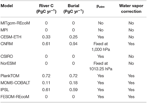
Table 1. Specifications of Global Ocean Biogeochemical Models: River carbon input, net burial and conversion from xCO₂ (ppm) to pCO₂ (μatm) using atmospheric sea-level pressure p_atm and water vapor correction.

The GOBMs do not consider river fluxes of carbon, alkalinity and nutrients into the ocean in the versions used here (MITgcm-REcoM, FESOM-REcoM, NorESM-OC, MPIOM-HAMOCC6, CSIRO) or their river fluxes are approximately balanced by burial in sediments (NEMO-PlankTOM5, IPSL, Princeton, CESM-ETHZ). In this case, these river fluxes do not induce a river-driven net sea-to-air CO₂ flux. Only in CNRM is the burial substantially larger than the lateral inflow of carbon into the ocean (Table 1).

2.2.1. GOBM Simulations and Analysis

Two simulations are performed by each modeling group. Simulation A is designed to reproduce the interannual variability and trend in the ocean carbon uptake in response to changes in both atmospheric CO₂ and climate. Simulation A is forced with interannual varying atmospheric forcing and increasing atmospheric CO₂. This is the contemporary CO₂ flux simulation and it includes the following terms:

$\begin{array}{ll}{\text{F}}_{\text{simA}}={\text{F}}_{\text{ant},\text{ss}}+{\text{F}}_{\text{ant},\text{ns}}+{\text{F}}_{\text{nat},\text{ss}}+{\text{F}}_{\text{nat},\text{ns}}+{\text{F}}_{\text{drift}+\text{bias}}& (4)\end{array}$

Simulation B is a control simulation with constant atmospheric forcing (normal year or repeated year forcing) and constant preindustrial atmospheric CO₂ (modeling groups use either 278 or 284 ppm). It represents the natural steady-state flux plus any flux due to bias and drift:

$\begin{array}{ll}{\text{F}}_{\text{simB}}={\text{F}}_{\text{nat},\text{ss}}+{\text{F}}_{\text{drift}+\text{bias}}& (5)\end{array}$

All models except CNRM and IPSL use a climatology or single year forcing for simulation B. Simulation B of CNRM is forced by cycling over the first 10 years of the NCEP/NCAR-R1 forcing. IPSL instead contributed a simulation with constant atmospheric CO₂ and interannual varying atmospheric forcing that corresponds to F_nat,ss + F_nat,ns + F_drift+bias.

In order to derive S_OCEAN from the model simulations, we subtract the annual time-series of simulation B from the annual time-series of simulation A for all models that used single year or climatological forcing for their simulation B. Assuming that F_drift+bias is the same in simulations A and B, we thereby correct for any model drift. Further, this difference also removes the F_nat,ss, which is often a major source of biases. Simulations B of IPSL and CNRM have to be treated differently due to their different protocols. For these models, we fit a linear trend to the simulation B and subtract this linear trend from simulation A. This approach assures that the interannual variability is not removed from IPSL simulation A. It will also remove a potential trend in F_nat,ns, which tends to be substantially smaller than the trend in F_ant,ss, but is still of potential interest in the context of decadal variability in the ocean carbon sink.

Modeling groups submit global and regional annual time-series of the ocean carbon sink integrated from their native model grids. This procedure avoids errors in the integrated carbon sink due to interpolation. These data are used for all time-series figures. Three regions are considered: north (>30°N), tropics (30°S-30°N) and south (<30°S). Further, gridded fields of pCO₂ and air-sea CO₂ flux on a 1x1 degree grid are used for model evaluation. The regional CO₂ fluxes are not corrected for bias and drift of the control simulation, as the assumption of zero F_nat,ss only holds on the global level. The submitted time-series and gridded fields for simulation A and B are published in the data repository Pangaea (Hauck et al., 2020).

2.3. Data-Based pCO₂ Mapping Methods

Three mapping methods are used here: the MPI-SOMFFN (Landschützer et al., 2016), the Jena-MLS (Rödenbeck et al., 2014), and the CMEMS (Denvil-Sommer et al., 2019) methods. The products are regularly updated, now covering the period 1982–2018 (Jena-MLS, MPI-SOMFFN) or 1985-2018 (CMEMS). All methods are based on SOCATv2019 surface ocean fugacity of CO₂ (pCO₂ corrected for the non-ideal behavior of the gas) as input data set, which is an update of SOCAT version 3 (Bakker et al., 2016). CMEMS used only two thirds of the SOCATv2019 data for training the method and the rest for validation. We refer to the resulting data sets as pCO₂-based data-products. From these gridded pCO₂ products, the contributing groups calculated the air-sea CO₂ flux using their own methods, and integrated their global and regional ocean carbon sink estimates over their native grids to provide the resulting air-sea CO₂ flux time-series. MPI-SOMFFN and CMEMS use the global monthly atmospheric xCO₂ time-series. Jena-MLS uses the spatially and temporally explicit xCO2 boundary conditions from the Jena Carbo Scope atmospheric inversion (Rödenbeck et al., 2018). All methods convert xCO₂ to pCO₂ using sea-level pressure and the water vapor correction. All three mapping methods use a quadratic gas-exchange formulation (k·U²·(Sc/660)^−0.5) with the transfer coefficient k scaled to match a global mean transfer rate of 16 cm/h (Wanninkhof, 1992; Naegler, 2009) and the Schmidt number Sc estimated with a third-order polynomial fit of sea surface temperature. The mapping methods use different wind speed products [Jena-MLS: NCEP/NCAR-R1 (Kalnay et al., 1996), MPI-SOMFFN: ERA-INTERIM (Dee et al., 2011), CMEMS: ERA5 (Hersbach et al., 2020; Simmons et al., 2020)] for the calculation of the CO₂ flux (Supplementary Table 1). Gridded fields of pCO₂ and air-sea CO₂ flux were submitted for the evaluation, where MPI-SOMFFN and CMEMS submitted monthly 1 × 1° fields. The daily 4 × 5° Jena-MLS fields were regridded to monthly 1 × 1° fields using nearest neighbor interpolation with the griddata function from the python SciPy module. The submitted time-series and gridded fields are published in the data repository Pangaea (Hauck et al., 2020).

The data-products are based on contemporary sea surface pCO₂ observations and thus estimate F_net (see Equation 1). In order to compare them with the S_OCEAN estimate, they have to be adjusted for the riverine flux F_riv,ss (using 0.78 ± 0.41 PgC yr⁻¹, Resplandy et al., 2018). The riverine adjustment is attributed to three latitudinal bands using the spatial distribution of Aumont et al. (2001) with the caveat that the regional boundaries are defined at 20°N and 20°S as opposed to the latitudinal boundaries of 30°N/S used in the GCB otherwise. This results in additive river flux adjustment terms of F_riv,ss of 0.20 PgC yr⁻¹ (north), 0.19 PgC yr⁻¹ (tropics), and 0.38 PgC yr⁻¹ (south).

2.4. Area Weighting

GOBMs and mapping methods all cover different amounts of ocean surface area. To close the Global Carbon Budget with CO₂ sources and sinks, the total ocean area has to be considered. Hence, the total ocean area covered by each GOBM and mapping method on their native grids was requested and compared to the global ocean area of 361,900,000 km² from ETOPO1 (Amante and Eakins, 2009; Eakins and Sharman, 2010).

The ocean area covered by the ocean models range between 352,050,000 km² for MITgcm-REcoM which excludes the Arctic north of 80°N to 365,980,000 km² for MPI. The ocean models hence cover 97.3–101.1% of the global ocean area. These differences in ocean coverage originate from the grid specifications in coastal regions, besides the missing Arctic and Mediterranean Sea in MITgcm-REcoM. As none of the models resolves coastal processes explicitly, we scale the annual time-series of the total ocean carbon sink by the ratio of the ETOPO1 global ocean area (Amante and Eakins, 2009; Eakins and Sharman, 2010) to the modeled ocean area.

The covered ocean area ranges from 88.9% of the global ETOPO1 ocean area in two data-products (MPI-SOMFFN and CMEMS) to 101.4% in the Jena-MLS. The non-mapped ocean area in MPI-SOMFFN and CMEMS are located all along the coasts and in marginal seas, including the Mediterranean Sea and the Arctic Ocean. We apply the same area-scaling procedure to the data-products as to the models to yield a consistent estimate of the global ocean carbon sink.

The areal correction is not applied to the regional fluxes due to the lack of information on area coverage per region. The effects of this area-correction or its omission are described and discussed in sections 3.2 and 4.5.

Global and regional time-series of GOBMs and data-products after area weighting but without river flux adjustment are archived in ICOS (Global Carbon Project, 2019).

2.5. Quantification of Temporal Variability

To quantify agreement of GOBMs and mapping methods on the multi-year variability of the GCB ocean sink estimate, we define four distinct periods. We chose the years 1992, 2001, and 2011 as boundaries for the four phases following Landschützer et al. (2015). These years also mark cusps in the ensemble mean of data-products, most pronounced in the Southern Ocean. We tested the trend significance within these multi-year periods from start year to end year with a Mann-Kendall test using the python module pyMannKendall (Hussain and Mahmud, 2019).

Furthermore, we calculate the amplitude of interannual variability (AIAV, Rödenbeck et al., 2015) as the temporal standard deviation of the air-sea CO₂ exchange derived from the gridded fields as follows: (1) air-sea CO₂ exchange filtered for water depth exceeding 400 m (not subsampled for SOCAT sampling sites), (2) spatially-integrated, (3) 12-months running mean filter applied, and (4) detrended. Our AIAV calculation differs from Rödenbeck et al. (2015) only by the detrending which is used to separate out the variability from the trend. It differs from the AIAV shown in Friedlingstein et al. (2019) by the detrending and also by the time period considered (1992–2018), which is shorter but has a larger data density.

2.6. Evaluation Metrics

We use the gridded pCO₂ fields for model evaluation on which we apply two filters. First, we follow Rödenbeck et al. (2015) by using only open ocean data points where water depth exceeds 400 m (thereby excluding 8% of the ocean area). Second, we subsample data-points from models and mapping methods for which there is a matching f CO₂ (fugacity of CO₂) value from the binned SOCATv2019 product (gridded, on a monthly 1 × 1° resolution; Bakker et al., 2016), which we refer to as pCO₂ in the following. The fugacity of CO₂ is 3–4‰smaller than the partial pressure of CO₂ (Zeebe and Wolf-Gladrow, 2001). We acknowledge the importance of this distinction in the observational community, but consider it negligible for the model evaluation.

We generate global and regional monthly mean pCO₂ time-series by averaging over all subsampled pCO₂ data points in a given region. All data points are weighted equally. Monthly correlation coefficient and root mean squared error (RMSE) between simulated and observed pCO₂ are calculated from the subsampled data sets before calculating the spatial average. Statistics are calculated for the period 1992–2018, due to the limited data availability of surface pCO₂ observations prior to 1992 (Bakker et al., 2016).

Annual time-series are calculated from the monthly mean subsampled time-series after integration over regions. Annual RMSE and correlation coefficient are calculated from these time-series, contrary to the monthly statistics. We consider this to be more robust than to calculate the annual mean at each pixel given the data sparsity. Hence, the annual metrics are to be interpreted as a measure of the misfit on the large regional or global spatial scale and on the multi-year time-scale (mean and trend). RMSE and correlation coefficient were additionally calculated from detrended annual mean time-series to separate out the mismatch of interannual variability on large spatial scales. For the GOBMs and data-products, a second annual time-series is calculated from the full data set to distinguish “true” variability from a potentially biased variability stemming from the sparse and inhomogeneous sampling.

The pCO₂ mismatch is calculated as simulated or mapped pCO₂ minus SOCAT pCO₂ at each data-point of the subsampled data set. It is then spatially averaged into a monthly time-series and temporally averaged into an annual time-series. The mean bias is calculated as the average of the annual mean mismatch.

3. Results

3.1. Control Simulation—Global and Regional CO₂ Flux

The ten GOBMs simulate a preindustrial ocean carbon sink F_nat,ss + F_drift+bias (simulation B) between −0.21 to 0.37 PgC yr⁻¹ with a mean of 0.1 PgC yr⁻¹ (0.08 PgC yr⁻¹ without FESOM as in Friedlingstein et al., 2019, a positive number indicates a flux into the ocean; Table 2, Figure 1). It follows from the definition of F_nat,ss = 0, that any deviation of CO₂ flux in simulation B from zero is considered a model bias. The drift of CO₂ flux in the control simulations varies between −0.0026 and 0.0034 PgC yr⁻² and is thus small compared to the trend of CO₂ flux in the historical simulation. The smallest drifts are found in two models with long spin-up (1,000 years, NorESM and MPI). CNRM and IPSL show more variability due to their forcing choices. FESOM-REcoM falls within the range of the other GOBMs with a positive bias and drift (Table 2).

TABLE 2

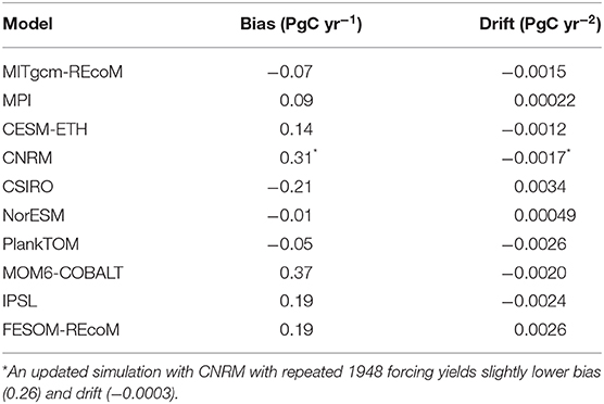
Table 2. Global bias and drift of annual air-sea CO₂ flux in control simulation of individual Global Ocean Biogeochemical Models. The drift is calculated as a linear fit to the full annual time-series 1959–2018.

FIGURE 1

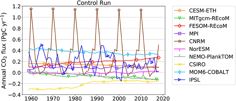
Figure 1. Annual air-sea CO₂ flux in control simulation (simulation B) of individual Global Ocean Biogeochemical Models. This is equivalent to F_simB = F_nat,ss + F_drift+bias (Equation 5), where any flux different from zero is considered a bias and any temporal change in the control simulation is considered a drift. Positive: CO₂ flux into the ocean.

The strong positive bias in CNRM can be explained by the burial flux which is larger than the river carbon input and leads to a CO₂ flux into the ocean in the preindustrial state. The burial is also larger than the river input in MOM6-COBALT, but not large enough to explain the bias of 0.37 PgC yr⁻¹. Other positive or negative biases cannot be explained by an imbalance of burial and river fluxes.

There are substantial natural CO₂ fluxes into and out of the ocean on a regional level that have previously been assessed using ocean inversions and ocean models (Mikaloff Fletcher et al., 2007). All GOBMs reproduce the natural CO₂ outgassing flux in the tropics, particularly the large flux to the atmosphere in the equatorial Pacific (Figure 2). There is less agreement on the relative contributions to natural CO₂ outgassing in the tropical Indian Ocean vs. the tropical Atlantic with a slightly larger contribution from the tropical Atlantic in MPI, NorESM, CSIRO, CESM-ETH, MOM6-COBALT, and FESOM-REcoM as in Mikaloff Fletcher et al. (2007). NEMO-PlankTOM simulates a much larger outgassing in the tropical Indian Ocean, whereas MITgcm-REcoM has close to zero flux and CNRM even a slight CO₂ uptake in the tropical Indian Ocean.

FIGURE 2

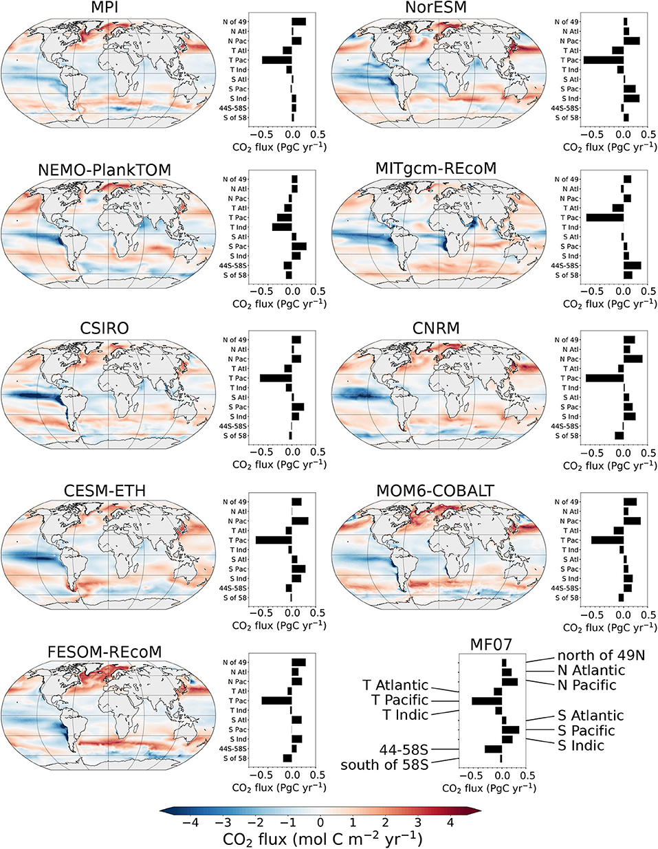
Figure 2. Natural air-sea CO₂ flux in individual Global Ocean Biogeochemical Models as derived from control simulation B. The air-sea CO₂ flux is averaged over the last 10 years of the control simulation. The bar plots exhibit integrated air-sea CO₂ fluxes over the regions used in Mikaloff Fletcher et al. (2007). The lower right bar plot shows the ocean inversion results from Mikaloff Fletcher et al. (2007, MF07). Positive numbers indicate a flux into the ocean.

There are differences between the models on the relative contributions of certain regions also in the northern extra-tropics, where the inversion showed the strongest CO₂ uptake in the low- and mid-latitude North Pacific, followed by the low- and mid-latitude North Atlantic and then high-latitudes (north of 49°N). This pattern is only reproduced by NorESM. Other models (MPI, CSIRO, CNRM, CESM-ETH, MOM6-COBALT, FESOM-REcoM) simulate a larger uptake in the high-latitudes than in the low- and mid-latitude North Atlantic. NEMO-PlankTOM5 and MITgcm-REcoM exhibit a small net outgassing signal in the low- and mid-latitude North Pacific or the low- and mid-latitude North Atlantic, respectively.

In the southern extra-tropics, the inversion exhibited CO₂ uptake with the strongest signal in the South Pacific, followed by the Southern Indian Ocean and the South Atlantic. This pattern is reproduced by NEMO-PlankTOM, CSIRO and CESM-ETH. Other models found a stronger CO₂ sink in the Southern Indian Ocean than in the Southern Pacific Ocean (NorESM, CNRM, MOM6-COBALT). In contrast, MPI and MITgcm-REcoM show weak outgassing signals in the South Pacific or South Atlantic, respectively. FESOM-REcoM produces a net zero flux in the South Pacific.

Previously identified discrepancies between ocean models and the ocean inversion estimates on the natural CO₂ flux prevail in the Southern Ocean (Mikaloff Fletcher et al., 2007, models: roughly zero flux, ocean inversion: outgassing). MPI and MITgcm-REcoM models have no net natural CO₂ outgassing in the regions 44–58°S or south of 58°S, all other models have net outgassing in at least one of these regions. The total natural CO₂ outgassing signal in the Southern Ocean is smaller in all models than in the ocean inversion.

3.2. Historical Simulation—Global CO₂ Flux

Since models are not scaled to the observational constraint of the 1990s anymore, their bias and drift as determined with the control simulation has to be subtracted to satisfy our definition of S_OCEAN. The mean correction applied in the GCB2019 (Friedlingstein et al., 2019) varies between −0.36 and +0.16 PgC yr⁻¹ when averaged over the 1990s and the multi-model mean CO₂ flux is thereby reduced by 0.07 PgC yr⁻¹. The correction leads to a larger model spread with a standard deviation of 0.27 PgC yr⁻¹. Similar reductions and larger spreads of the ensemble mean CO₂ flux result for other time periods, e.g., a reduction of 0.06 and 0.05 PgC yr⁻¹ for the 2000s and the period 2009–2018, respectively (Table 3).

TABLE 3

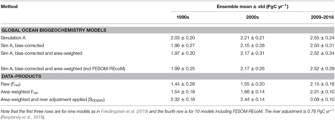
Table 3. Ensemble mean and standard deviation of air-sea CO₂ flux before and after applying corrections.

To close the Global Carbon Budget, the total ocean area has to be considered, and we scale all GOBMs to the same global ocean area. This has a small effect on the ocean carbon sink estimate with corrections of −0.02 PgC yr⁻¹ for the MPI model to +0.05 PgC yr⁻¹ for MITgcm-REcoM, when averaged over the 1990s. The multi-model mean increases by 0.01, 0.01, and 0.02 PgC yr⁻¹ when averaged over the 1990s, 2000s, and 2009–2018, respectively (Table 3). The model spread is further enlarged as the CO₂ flux in the MPI model which has already the lowest ocean carbon sink, is further reduced and the CO₂ flux in the two models with the largest ocean carbon sink (CSIRO, NorESM) is further increased.

Taken together, the bias-correction and area-weighting reduce the multi-model mean ocean carbon sink estimate slightly and increase the model spread (Table 3). All models are within the observational constraint of anthropogenic ocean CO₂ uptake for the 1990s of 2.2 ± 0.6 PgC yr⁻¹ before and after applying these corrections. This observational constraint is based on an assessment taking into account indirect observations with seven different methodologies (Denman et al., 2007). These methods include the observed atmospheric O₂/N₂ concentration trends (Manning and Keeling, 2006; Keeling and Manning, 2014), an ocean inversion method constrained by ocean biogeochemistry data (Mikaloff Fletcher et al., 2006), and a method based on chlorofluorocarbons (McNeil et al., 2003). In the GCB, the confidence interval was adjusted to 90% to avoid rejecting models that may be outliers but are still plausible (2.2 ± 0.6 PgC yr⁻¹, Friedlingstein et al., 2019).

The spread in the covered ocean area is larger in the data-products than in the GOBMs and area-scaling has a pronounced effect on their ocean carbon sink estimate. The area-scaling changes the 1990s ocean carbon sink by +0.15, −0.02, and +0.18 PgC yr⁻¹ in MPI-SOMFFN, Jena-MLS, and CMEMS, respectively. The ensemble mean increases by 0.10 PgC yr⁻¹ and the standard deviation is substantially reduced from 0.26 to 0.18 PgC yr⁻¹ (Table 3). The area-weighting effect increases over time to 0.16 PgC yr⁻¹ over the period 2009–2018. The standard deviation of the data-products decreases over time, but is still reduced by a third through area-weighting in the decade 2009–18.

The ocean carbon sink estimate from data-products is the contemporary CO₂ flux, hence an adjustment for the preindustrial CO₂ outgassing due to river carbon flux has to be applied to comply with S_OCEAN. The river flux adjustment of 0.78 ± 0.41 PgC yr⁻¹ (Resplandy et al., 2018) to the data-products results in a larger ocean carbon uptake compared to the GOBMs. The data-products mean of 2.32 ± 0.18 PgC yr⁻¹ (±1 standard deviation) of the 1990s falls within the observational constraint for the 1990s. The discrepancy between model and data-based estimates varies between 0.35 PgC yr⁻¹ in the 1990s and 0.27 PgC yr⁻¹ in the 2000s, to 0.57 PgC yr⁻¹ in 2009–2018, and 0.82 PgC yr⁻¹ in the last year 2018. The uncertainty in the river flux adjustment of ±0.41 PgC yr⁻¹ (Resplandy et al., 2018) can explain a large part of the mean discrepancy. Due to a backlog in submissions to the SOCAT database, the total amount of observations used to constrain the last year has a third less observations (1.3 million observations in 2019 and 2 million observations in 2018) than in previous years. Therefore, 2018 also shows quite a remarkable spread between the mapping methods.

The models generally simulate an enhanced CO₂ uptake during El Niño events, though not all models show a response to all strong and very strong El Niño events (e.g., NorESM and MPI El Niño 1997/98, Figure 3 lower panel). Models and data-products show the same patterns of variability, but differences exist in the mean S_OCEAN and in the decadal trends. This is particularly pronounced since 2005, but also applies to earlier decades 1980–2000 (Figure 3). While the uncertainty in the river flux adjustment can account for a large part of the mean discrepancy, it cannot explain the difference in trends since 2005. The discrepancy in trends could only be explained through the riverine term by a reduced riverine outgassing over time, which would mean a reduced river carbon inflow into the ocean under the assumption of a constant ratio of river carbon inflow to riverine outgassing. There is, however, no indication of a decreased river transport of carbon into the ocean (Regnier et al., 2013).

FIGURE 3

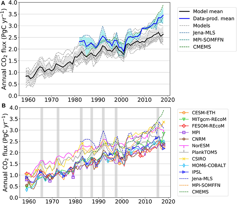
Figure 3. Annual air-sea CO₂ flux from Global Ocean Biogeochemistry Models (GOBMs) and data-products used in the Global Carbon Budget 2019, after applying bias and area-corrections and river flux adjustment of 0.78 PgC yr⁻¹ (Resplandy et al., 2018). (A) Mean of model ensemble and data-product ensemble as thick lines, individual models and data-products as thin dashed lines. (B) Individual models and data-products in color. Gray bars indicate strong and very strong El Niño events with the extended Multivariate ENSO index (MEI) being above 1.5 for at least 3 months in a row (Wolter and Timlin, 2011). Positive numbers indicate a flux into the ocean.

3.3. Historical Simulation: Regional CO₂ Flux

Separating the global S_OCEAN into large-scale regional bands reveals substantial differences in our understanding of the mean ocean carbon sink and its variability. In the tropics, GOBMs and data-products agree well on the mean of S_OCEAN and its variability (Figure 4). Models simulate a mean uptake of 0.01 PgC yr⁻¹ in 2018 with a spread from outgassing of 0.16 PgC yr⁻¹ in NEMO-PlankTOM to an uptake of 0.32 PgC yr⁻¹ in CNRM. The data-products agree on a small tropical CO₂ sink of 0.04–0.19 PgC yr⁻¹. The ensemble of data-products and GOBMs agree that the tropics are in the process of turning from a CO₂ source to a CO₂ sink. The first occurrence of the tropical CO₂ sink was in 2015 in the data-product ensemble and in 2014 in the GOBM ensemble.

FIGURE 4

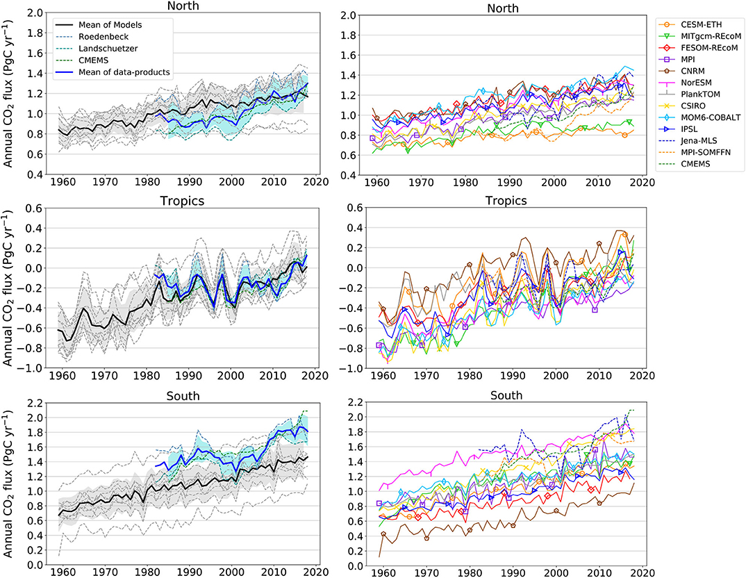
Figure 4. Annual air-sea CO₂ flux integrated over the regions North (north of 30°N, top), Tropics (30°S-30°N, center), South (south of 30°S, bottom). These time-series are taken from the historical simulation A and are not corrected for biases or covered area. Note the different scales for different regions. Horizontal lines have the same distance in all subfigures (0.2 PgC yr⁻¹). Positive: CO₂ flux into the ocean. Left: Ensemble mean of Global Ocean Biogeochemical Models and data-products. Individual models in gray. Right: Individual models and data-products color coded.

In the north, GOBMs simulate a CO₂ sink of 0.85–1.45 PgC yr⁻¹ in 2018. Seven models and all data-products fall within an envelope of 1.15–1.45 PgC yr⁻¹. The CO₂ sink in the MITgcm-REcoM set-up without the Arctic and CESM are lower with 0.89 and 0.85 PgC yr⁻¹, respectively, and stagnate since 2000. The data-product ensemble mean yields a CO₂ sink lower than the model ensemble mean by 0.1–0.2 PgC yr⁻¹ between 1985 and 2001 and good agreement since 2005.

The largest model spread occurs in the Southern Ocean with the models simulating a CO₂ sink between 1.11 PgC yr⁻¹ (CNRM) and 1.84 PgC yr⁻¹ (CSIRO) in 2018. Six models fall in an envelope of 1.16–1.50 PgC yr⁻¹. One model (CNRM) is lower than the multi-model mean by about 0.3 PgC yr⁻¹ throughout the entire period, although it comes closer in 2018 with a simulated sink of 1.11 PgC yr⁻¹. Two models are higher with NorESM simulating higher CO₂ uptake by about 0.3 PgC yr⁻¹ throughout the entire period with 1.78 PgC yr⁻¹ in 2018 and CSIRO branching off the other models in 1980 to reach 1.84 PgC yr⁻¹ in 2018. The data-products have the largest temporal variability and different patterns of interannual variability in the south and result in CO₂ uptake estimated between 1.67 and 2.09 PgC yr⁻¹ in 2018, after river flux adjustments. The data-product mean is higher by 0.3 PgC yr⁻¹ than the model ensemble mean. The only exception is the early 2000s where the data-product mean comes close to the model ensemble mean due to the low CO₂ sink in the MPI-SOMFFN product in the late 1990s and early 2000s. The Jena-MLS exhibits similar variability but on a higher mean level and the CMEMS and the GOBMs show weaker internannual and multi-year variability.

The ocean carbon sink in FESOM-REcoM is close to the multi model mean globally and in the tropics. The simulated ocean carbon uptake in the north is at the high end of the simulated range, clustering with the CNRM, NorESM, MOM6-COBALT, and IPSL models. In the south, FESOM-REcoM is in the lower range of simulated carbon uptake, but still on average 0.24 PgC yr⁻¹ above CNRM.

3.4. Historical Simulation: Multi-Year Variability of CO₂ Flux

All models and data-products show a slower growth or stagnation of the ocean sink in the 1990s and a reinforcement in the 2000s (Figure 3). Here, we test the consistency of multi-year variability of the ocean carbon sink among the GOBMs and the data-products in the three regions (Figure 5). We use the term multi-year variability to describe variability on a time-scale longer than interannual variability (1–3 years), but not strictly restricted to a decade (decadal variability, DeVries et al., 2019).

FIGURE 5

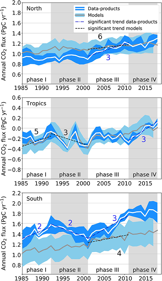
Figure 5. Multi-year variability of regional air-sea CO₂ flux with agreement among methods on no significant or a decreasing trend in phase II and an increasing trend in the extratropics in phase III. Shown are the average and standard deviation of annual CO₂ flux for the ensemble of data-products and the ensemble of Global Ocean Biogeochemical Models (GOBMs) in the north (top), tropics (center) and south (bottom). Broken lines represent significant trend over that time-period. Numbers indicate the number of individual data-products and GOBMs that agree on the significant trend and are only given if the trend of the ensemble average is also significant. Note the different scales for different regions. Horizontal lines have the same distance in all subfigures (0.2 PgC yr⁻¹). Positive: CO₂ flux into the ocean.

In the data-products, phase I (1985–1992) is characterized by a positive trend in the south (p = 0.013) and no significant trends in the tropics and the north. The significant trend for the south in the data-products does not coincide with a significant trend in the models. The model ensemble mean also suggests a positive trend in the tropics, although with less certainty (p = 0.036). It is noteworthy that there is least confidence in data-products in phase I due to lower data availability, and the highest confidence in phases III and IV.

In phase II (1992–2001), the trend in the south is reversed (p = 0.001) in the data-product ensemble, and is zero in the north and in the tropics. The model ensemble mean also suggests a negative trend in the tropics, although with less certainty (p = 0.032). The significant trend for the south in the data-products does not coincide with a significant trend in the models. Although there are discrepancies on whether or not the ocean carbon sink was decreasing, GOBMs and data-products agree remarkably well on the slow-down or stagnation of the ocean carbon sink in phase II (1992–2001) with no GOBM or data-product exhibiting a significantly increasing trend. All GOBMs and data-products agree on the absence of a significant trend in the north.

Phase III (2001–2011) is again characterized by a sign reversal and strong positive trend in the south (p = 0.006) in the data-product ensemble mean, accompanied by a positive trend in the north (p = 0.006) and no trend in the tropics with a remarkable agreement of all data-products. The model ensemble mean agrees with positive trends of CO₂ flux in the north (p = 0.008) and south (p = 0.020).

Finally, in phase IV (2011–2018) the data-product ensemble mean exhibits a positive trend in the tropics (p = 0.004), which is however only matched by one GOBM out of the full ensemble. The ensemble means of data-products or GOBMs indicate no significant trend in the north and south, although few individual GOBMs and data-products do so. Phase IV is shorter than the other phases and therefore potentially less conclusive.

While models and data-products agree on the large-scale (quasi-)decadal variability (Figure 5), the strength of the interannual variability and its hot spots differ largely (Figures 6, 7 y-axis). Among the data-products, MPI-SOMFFN and CMEMS show similar patterns of variability with the largest amplitude of interannual variability per pixel in the subpolar regions of all basins and the equatorial Pacific (Figure 6). The same spatial pattern although generally higher variability is visible in the Jena-MLS product. The data-products generally distribute the variability roughly equally between these regions. In the model suite, only MOM6-COBALT and MITgcm-REcoM distribute the variability similarly among these regions, although in MITgcm-REcoM the variability is not limited to these regions. Some models place most of the variability in the tropical Pacific (CSIRO, PlankTOM, CESM-ETH, NorESM), in other models the northern subpolar regions and the equatorial Pacific are dominant regions of variability (FESOM-REcoM, IPSL and CNRM). MPI exhibits strong variability in the Southern Ocean and the North Atlantic.

FIGURE 6

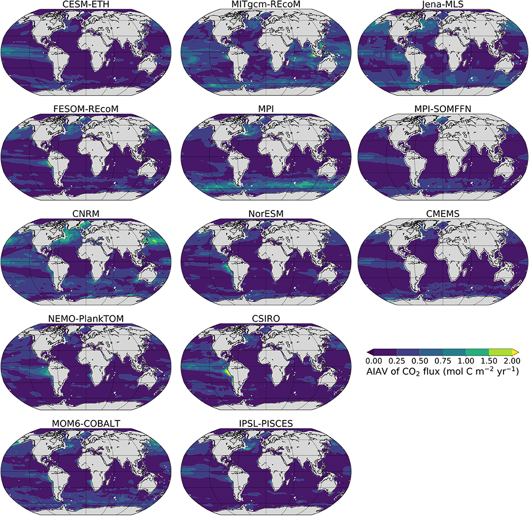
Figure 6. Spatially resolved amplitude of interannual variability (AIAV) of annual air-sea CO₂ flux calculated as the standard deviation of the detrended annual CO₂ flux for all GOBMs and data-products.

FIGURE 7

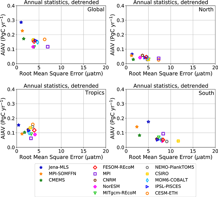
Figure 7. Summary figure of temporal variability (y-axis) and model-data mismatch (x-axis). Mismatch of simulated or mapped pCO₂ and observed sea surface pCO₂ for the period 1992–2018 on the time-scale of multi-year variability and amplitude of interannual variability (AIAV) of CO₂ flux. x-axis: RMSE of spatially-averaged detrended annual time-series. y-axis: amplitude of interannual variability, defined as the standard deviation of the detrended annual time-series of air-sea CO₂ flux. These statistics are shown globally, and regionally for north, tropics, and south as indicated in the figure panels.

The amplitude of interannual variability (AIAV) of the global and regional CO₂ flux time-series of GOBMs and data-products is summarized in Figure 7 (y-axis). The interannual variability as reproduced by GOBMs and data-products fall into similar ranges in the north (0.02–0.08 PgC yr⁻¹) and in the tropics (0.05–0.16 PgC yr⁻¹). There is disagreement among GOBMs and data-products on the AIAV in the south with the data-products varying between 0.08 and 0.18 PgC yr⁻¹ while all GOBMs are below 0.1 PgC yr⁻¹.

3.5. Historical Simulation: Model and Data Comparison

Model evaluation was introduced as a single mismatch metric using monthly surface ocean pCO₂ observations from the Surface Ocean CO₂ Atlas (SOCAT, Bakker et al., 2016) in Le Quéré et al. (2018a, their Figure B1). Here, we show a detailed model-data comparison for models and data-products with the SOCAT pCO₂ data set on three time-scales: (i) monthly, (ii) annual + trend, and (iii) multi-year variability. The latter is the approach most closely quantifying interannual to multi-year variability, and therefore, we argue, the most appropriate metric for the Global Carbon Budget, with the aim to quantify the mean S_OCEAN and the deviation from previous years (i.e., multi-year variability).

Annual time-series of subsampled pCO₂ from GOBMs and data-products are compared to SOCATv2019 for the ensemble mean of the GOBMs and data-products (Figure 8 with statistics on annual + trend time-scale), and for all individual models and data-products in the Appendix (Supplementary Figures 3–15). The data-products follow the SOCAT pCO₂ closely, with the best agreement in the tropics (RMSE = 2.0 μatm, r = 0.991, Figure 8), followed by the north (RMSE = 4.0 μatm, r = 0.985), and slightly lower agreement in the south (RMSE = 5.5 μatm, r = 0.968). As expected, the average of the subsampled pCO₂ of the data-products deviates from the average of the fully gridded product. It is, however, remarkable, that this difference is smallest in the north and largest in the south, confirming that data coverage is best in the north and sampled pCO₂ can represent the entire area reasonably well. In the tropics and the south, larger differences between subsampled mean pCO₂ and average over the full domain suggest that data coverage is insufficient to adequately represent these large areas.

FIGURE 8

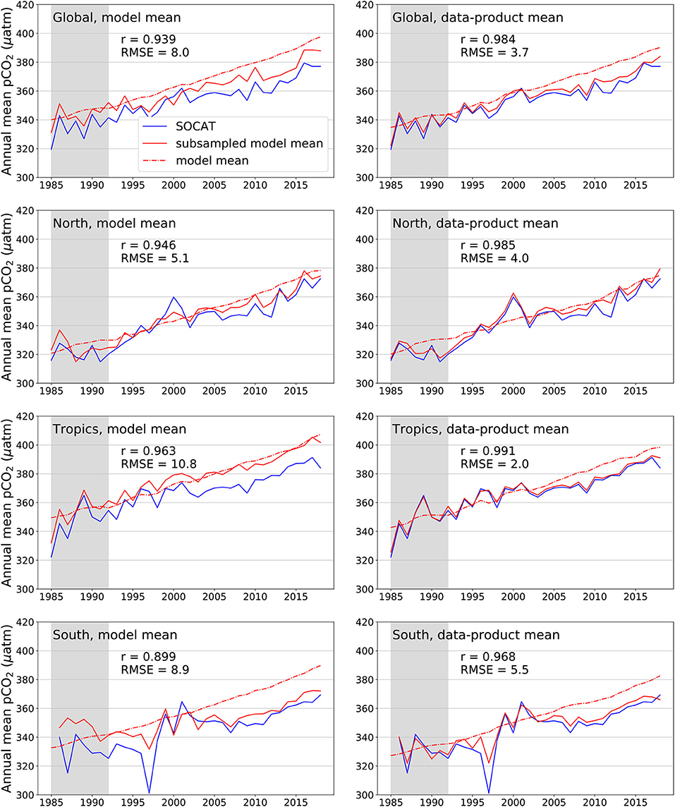
Figure 8. Comparison between annual sea-surface pCO₂ from SOCATv2019 (Bakker et al., 2016) and the model ensemble mean (left) or data-product ensemble mean (right) globally (top), and in the different regions North, Tropics, South as indicated in the figures. Red solid line shows model or data-product mean from subsampled models/data-products at SOCAT sampling sites. Broken lines indicate the area-weighted average from the full models (not subsampled). Correlation coefficient r and Root Mean Squared Error RMSE are calculated from the annual time-series 1992–2018, i.e., the white area in the figures. These figures are shown for all models and data-products separately in the Supplementary Material.

The subsampled GOBM pCO₂ captures the variability of SOCAT pCO₂ remarkably well (Figure 8), given that SOCAT pCO₂ is an independent data set for the models. The model ensemble mean shows the highest correlation in the tropics (r = 0.963), but the lowest RMSE in the north (5.1 μatm). While the high correlation in the tropics indicates that the variability is well-captured, the RMSE is higher here as the water vapor correction, which is not included in some models, has a stronger effect at higher temperatures (see discussion on mean bias below). It is noteworthy that the mismatch between modeled and observed pCO₂ in the south is lower since 1999. Similar to the data-products, the difference between subsampled and full domain average pCO₂ is largest in the south.

In the following, we will show that the RMSE in comparison with SOCAT pCO₂ time-series is smaller on the relevant time-scale of multi-year variability (GOBMs: <10 μatm, data-products: <5 μatm, Figure 9) than on the time-scale annual + trend (GOBMs: <20 μatm, data-products: <7 μatm) and substantially smaller than on the monthly time-scale (GOBMs: 20–80 μatm, data-products: <20 μatm).

FIGURE 9

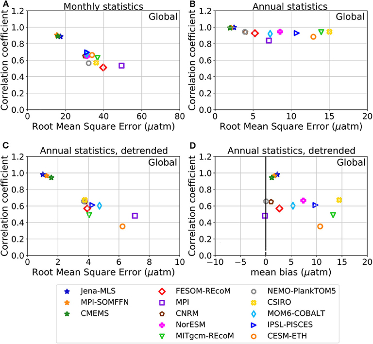
Figure 9. Mismatch of simulated or mapped pCO₂ and observed sea surface pCO₂ for the period 1992–2018 on different time-scales: (A) monthly, (B) annual + trend as derived from annual statistics, (C) multi-year variability as derived from detrended annual statistics, (D) long term mean. (A–C) Display the mismatch as RMSE and correlation coefficient. In (D) the mean bias is plotted against the correlation coefficient. Global figures are shown here, regional figures (north, tropics, south) are displayed in the Supplementary Material. Note the different scales on the x-axis.

The monthly means of modeled surface ocean pCO₂ cover a large range of simulated realizations, from smaller (e.g., PlankTOM, north, Supplementary Figure 6) to larger seasonal cycles (e.g., MPI, south, Supplementary Figure 4) compared to the observations, pointing to model deficiencies in representing the seasonal cycle correctly, especially in the Southern Ocean (Kessler and Tjiputra, 2016; Mongwe et al., 2016, 2018). Most models exhibit larger variability than in the observations on a monthly basis. This is mirrored in correlations of modeled and observed monthly pCO₂ ranging from 0.2 to 0.8 and the RMSE from 20 to 80 μatm (Figure 9A and Supplementary Figure 1). The data-products are inter- and extrapolations of SOCAT data, and hence have higher correlation coefficients and lower RMSEs than the GOBMs. However, they also have RMSEs of 15–20 μatm (see also Gregor et al., 2019) and correlation coefficients of 0.8–1.0 with lower correlation values in the southern and northern extratropics (Figure 9A, Supplementary Figures 1, 3–15 for individual models and data-products). Comparison on monthly time-scales is a common approach to measure misfit between estimated and observed pCO₂ (e.g., Le Quéré et al., 2018a; Friedlingstein et al., 2019; Gregor et al., 2019).

On the time-scale annual + trend, correlations for annual time-series are between 0.8 and 1 for all models, except in the Southern Ocean with values down to 0.6 (Figure 9B and Supplementary Figure 1). Despite all models having similarly high correlation values, the RMSEs range between 4 and 20 μatm. Data-products have correlation coefficients close to 1 and RMSE lower than 4 μatm. As the pCO₂ signal on the annual + trend time-scale is dominated by the continuous atmospheric CO₂ increase, we conclude that models and data-products capture the climate trend of increasing surface pCO₂ reasonably well.

Finally, on the time-scale of interannual and multi-year variability (statistics of detrended annual time-series, Figures 7, 9C, and Supplementary Figure 2), RMSEs between GOBMs and SOCAT are small (globally: 3.5–7 μatm); with the lowest mismatch in the tropics (2–4 μatm), and the largest mismatch in the south (6.5–9.5 μatm). On this time-scale, correlation coefficients are generally higher for GOBMs with lower RMSE, with highest correlation coefficients in the tropics (0.5–0.9) and lower in the extratropics (0.2–0.9 in the north and 0.2–0.8 in the south). The data-products are by design closer to the observations and have RMSEs below 2 μatm, except in the Southern Ocean with RMSEs up to 5 μatm, and correlation coefficients of above 0.8 in the south and above 0.9 elsewhere. The data-products cluster closely together in the north, with a wider range in the tropics and the south; again suggesting that data-availability can constrain the data-products better in the north than elsewhere.

The mean bias (Figure 9D, x-axis) is a measure of how well the models capture the mean pCO₂. It ranges between −1 and +15 μatm globally and up to 20 μatm in the tropics. Some models show a consistent positive bias as expected from the missing water vapor correction. The water vapor correction would reduce the modeled pCO₂ by 2 μatm at 0°C and by 15 μatm at 30°C. Including the water vapor correction in all models would substantially reduce the bias and would therefore allow for more detailed interpretation of model biases, e.g., in comparison to the regional CO₂ flux in the preindustrial control simulation. The mean bias of the data-products is always positive and small by design with a maximum of 5 μatm in the south.

4. Discussion

The ocean mitigates climate change by sequestering anthropogenic CO₂. A high-quality assessment of the ocean carbon sink is critical for assessing changes in the contemporary carbon cycle and to robustly project its evolution into the future. Sudden changes in the ocean carbon sink would immediately affect the allowable emissions for limiting global warming to well below 2°C. Furthermore, reliable quantification of the ocean carbon sink is also an important constraint on the land carbon sink estimate when combined with accurately reported emissions. The latter contributes 60–90% of the observed decadal variability in the natural carbon sinks (DeVries et al., 2019), but cannot be directly observed.

The ocean carbon cycle community is blessed with an annually-updated global compilation of quality-controlled surface ocean pCO₂ observations (the Surface Ocean CO₂ Atlas, SOCAT, Bakker et al., 2016), which can be used to derive the ocean carbon sink and to evaluate global ocean biogeochemical models (GOBMs). The ocean carbon sink can be assessed currently within <2 years delay through ocean surface pCO₂ observations combined with mapping methods and additional data sets and parameterizations, and by global ocean biogeochemical models. We demonstrated that these different tools agree reasonably well when enough high-quality observations are available. It has to be noted though, that the discrepancy between GOBMs and data-products is increasing over time, being larger in 2018 than in any year before.

The biggest discrepancies exist in the Southern Ocean, where model biases are largest and high-quality ship-board measurements are scarce and biased toward summer. Novel autonomous methods are starting to fill data gaps, e.g., pH sensors on biogeochemical Argo floats in the Southern Ocean (Bushinsky et al., 2019), but the uncertainty of calculated pCO₂ from pH sensors is higher than from direct pCO₂ observations (Williams et al., 2017). A global-scale high-quality ocean pCO₂ observation network combining traditional and novel observation systems is needed to improve the accuracy of the ocean carbon sink from observations.

4.1. The Mean Ocean Carbon Sink

The GOBMs best estimate for the mean ocean carbon sink is 2.1 ± 0.5 PgC yr⁻¹ between 1994 and 2007, which is 0.5 PgC yr⁻¹ lower than a recent anthropogenic carbon estimate of 2.6 ± 0.3 PgC yr⁻¹ based on ocean interior observations (Gruber et al., 2019). The two estimates overlap within the given uncertainties. More importantly, the 2.6 ± 0.3 PgC yr⁻¹ in Gruber et al. (2019) is equivalent to the geochemical increase in ocean inorganic carbon or F_ant,ss + F_ant,ns (Clement and Gruber, 2018). Gruber et al. (2019), however, also estimate outgassing of natural carbon, F_nat,ns, to be −0.4 ± 0.24 PgC yr⁻¹ over the same period. This is based on the difference of the net flux from a data-product (Landschützer et al., 2016) adjusted for riverine outgassing (i.e., F_ant + F_nat = F_net − F_riv) and two estimates of temporally-resolved F_ant [transient steady state scaled Landschützer et al. (2016) and ocean inversion Mikaloff Fletcher et al., 2006]. Hence, in order to compare the same conceptual S_OCEAN flux (F_ant,ss + F_ant,ns + F_nat,ns, Equation 2), the GOBM's S_OCEAN estimate has to be compared with the sum of Gruber's F_ant and F_nat,ns fluxes; and the resulting 2.2 ± 0.4 PgC yr⁻¹ are in good agreement with the numbers presented here and in the GCB releases (Friedlingstein et al., 2019). It is not a circular argument to use Gruber's F_ant plus F_nat,ns to compare to the GOBMs which are independent of both the F_ant and F_nat,ss estimates in Gruber et al. (2019). There would be some circularity when comparing to the data-based products, which is not done here.

On a regional level, global ocean biogeochemical models and data-products agree reasonably well on the mean ocean carbon sink in the tropics and in the northern exratropics. An exception to that is the offset between 1985 and 2003 in the northern extratropics. The better agreement since the early 2000s coincides with a large increase in number of (global) observations from 400,000 to 1,300,000 observations between 2003 and 2006 (Bakker et al., 2016), and a jump from a few hundred to a few thousand observations in the North Atlantic in 2002 (Lebehot et al., 2019). There is substantial disagreement on the mean ocean carbon sink in the Southern Ocean between GOBMs and data-products. This offset might be related to the high uncertainty of the river-flux adjustment, to an overestimate of the ocean carbon sink based on SOCAT observations due to a sampling bias or to model biases. Bushinsky et al. (2019) demonstrated that adding biogeochemical Argo floats to the input data set for two of the three mapping methods used here, reduces the Southern Ocean carbon sink by 0.39–0.75 PgC yr⁻¹ south of 35°S due to added winter-time data with previously underrepresented outgassing of CO₂. However, a systematic bias of 4 μatm well within the float pCO₂ uncertainty of around 11 μatm (Williams et al., 2017) would half the impact of the additional data from floats (Bushinsky et al., 2019). The global river flux adjustment (Resplandy et al., 2018) is distributed across the ocean based on one ocean circulation model study (Aumont et al., 2001). How much CO₂ outgasses in which ocean region depends on model assumptions, such as the remineralization time-scale of organic carbon and the burial. Further sensitivity studies on the effect of model assumptions are needed to constrain the regional river flux adjustments better.

4.2. Multi-Year Variability of the Ocean Carbon Sink

There is growing evidence for a multi-year variability of the ocean carbon sink with remarkable consistency among data-products and GOBMs on a global stagnation of the ocean carbon sink in the period 1992–2001 and an extra-tropical strengthening between 2001 and 2011 (Figure 5, Rödenbeck et al., 2015; Landschützer et al., 2016; DeVries et al., 2019; McKinley et al., 2020). Explanations for this multi-year variability range from the ocean's response to changes in atmospheric circulation (Le Quéré et al., 2007; Landschützer et al., 2015; Keppler and Landschützer, 2019), especially the variations in the upper ocean overturning (DeVries et al., 2017) to external forcing through surface cooling associated with volcanic eruptions and variations in atmospheric CO₂ growth rate (McKinley et al., 2020). The mapping methods and an ocean inverse model suggest that the GOBMs underestimate the magnitude of the multi-year variability (DeVries et al., 2019). Cooling due to volcanic eruptions and variations in atmospheric growth rate are included in the model forcing and the ocean circulation's response to climate variability is part of the model dynamics. Which of the two is the dominant factor is not distinguished in our analysis.

In the most recent period since 2011, all data-products yield a strong increasing trend of S_OCEAN in the tropics. This is not reproduced by the GOBMs, even though they generally represent the same amplitude of interannual variability (AIAV) as the data-products (Figure 7). In the northern extra-tropics, the AIAV of the data-products is smallest of all regions (<0.08 PgC yr⁻¹), but nevertheless varies by a factor of two between the data-products. The GOBMs fall within the same range. In the southern extratropics, the magnitude of the variability is by no means understood, with a large range of AIAV among data-products and GOBMs.

4.3. Lessons Learned From pCO₂ Data Mismatch

The pCO₂ data mismatch has to be interpreted in the context of high spatial and temporal ocean pCO₂ variability. The 1998–2011 mean pCO₂ varies spatially between 280 μatm in the high-latitude North Atlantic and North Pacific to over 440 μatm in the equatorial Pacific (Landschützer et al., 2014). Seasonal and interannual variability of surface pCO₂ can be 100 μatm or more (Wanninkhof et al., 2013). The zonal mean ΔpCO₂, i.e., the difference between surface ocean pCO₂ and atmospheric pCO₂ ranges from 40 μatm just south of the equator (outgassing) to −20 μatm at 40° of both hemispheres and −60 μatm (uptake) in the northern high latitudes (Wanninkhof et al., 2013). The global mean ΔpCO₂ varied only between −2 to +1 μatm between 1990 to 2009 according to Wanninkhof et al. (2013) and between −3 to 1 μatm from 1982 to 2000 and have since then increased to −6 μatm in the MPI-SOMFFN data-product used here (not shown). Over the same period, the global mean CO₂ flux has always been into the ocean and has not changed sign in the same product. This illustrates that the global mean ΔpCO₂ is dominated by the large areas in the tropics whereas the CO₂ flux is dominated by the subpolar regions with the highest wind speeds. We conclude from this context, that it is difficult to quantify an uncertainty of the CO₂ flux based on the pCO₂ bias or RMSE, but that it is encouraging that the GOBMs show only slightly weaker correlation with the SOCAT pCO₂ (0.94 globally) than the data-products (0.98) indicating that interannual and multi-year changes are captured reasonably well (Figure 8).

The detailed comparison of mapped and simulated pCO₂ with SOCAT data at sampling locations reveals that there is no relation between the RMSE or bias of the GOBM or data-product with the magnitude of temporal variability (Figure 7). We can therefore not constrain the “true” multi-year variability by choosing models with lower pCO₂ biases. Our analysis further assesses the fidelity of the GOBMs and data-products on different time-scales. While GOBMs have clear weaknesses on resolving the seasonal cycle (Figure 7A, Supplementary Figures 1, 3–15, Kessler and Tjiputra, 2016; Mongwe et al., 2016, 2018), they capture the pCO₂ on annual + trend time-scale reasonably well, and even better on the time-scale of multi-year variability (Figures 7, 9, and Supplementary Figure 2). We argue that the detrended annual statistic is more informative for the evaluation of annual estimates of S_OCEAN with the aim to robustly estimate the mean S_OCEAN and multi-year variability. The monthly statistics, which are most commonly used to evaluate GOBMs and data-products (Rödenbeck et al., 2015; Friedlingstein et al., 2019; Gregor et al., 2019) quantify to a large extent the representation of the seasonal cycle. Based on our analysis of model-data mismatch, we conclude that misrepresentations of the seasonal cycle in GOBMs have little effect on the global annual estimate of S_OCEAN. Yet, they illustrate the weaknesses of GOBMs to represent the underlying mechanisms correctly, which questions their ability to produce robust projections into the future.

4.4. Constraints on the Regional CO₂ Flux

Some models are clear outliers in the regional S_OCEAN time-series, e.g., CESM and MITgcm show the lowest S_OCEAN in the north, CNRM shows the highest flux in the tropics, and CNRM and NorESM exhibit a very low and very high S_OCEAN in the south, respectively. These models simulate very similar RMSEs and correlation coefficients in comparison to SOCAT pCO₂ as the other GOBMs and hence the regional fluxes cannot be constrained by the pCO₂ mismatch. In fact, CNRM shows the lowest RMSE in the south and in the tropics, but this assessment is hampered by the large global S_OCEAN bias in CNRM.

Similarly, the regionally resolved comparison of the preindustrial control air-sea CO₂ flux with ocean inversion estimates (Mikaloff Fletcher et al., 2007) is not conclusive on which models are more realistic than others, e.g., there is no obvious explanation for the low S_OCEAN in CESM in the north to be found in the preindustrial air-sea CO₂ flux in CESM in this region. However, a few impressions can be noted. MITgcm and MPI have clear issues with no net CO₂ outgassing in the preindustrial Southern Ocean. Models with a high CO₂ uptake in the north show this also in the preindustrial simulation (NorESM, CNRM, MOM6-COBALT, FESOM-REcoM), indicating that the model set-up and parameter choices lead to a vigorous overturning in the north. CNRM and FESOM-REcoM, which simulate the lowest historical S_OCEAN in the south, are the models with the strongest preindustrial outgassing south of 58°S, but still lower than in Mikaloff Fletcher et al. (2007).

4.5. Changes in Methodology in GCB2019

GOBMs have biases and they drift, which can be quantified with a control simulation that is required for the GCB since 2019 (Friedlingstein et al., 2019). The global ocean carbon sink estimate for the GCB can be corrected for model bias and drift and the effect of this correction is small on the ensemble global mean sink as some GOBMs have positive and others negative biases. Regional and subregional biases are, however, not quantified and cannot be corrected for as the assumption of net zero steady state natural flux only holds globally. Therefore, regional estimates of S_OCEAN are associated with a higher uncertainty and uncorrected gridded fields from historical model simulation A are used for model evaluation. This introduces an inconsistency between adjusted global estimates for S_OCEAN on the one hand and unadjusted regional S_OCEAN estimates and model evaluation on the other hand. Model simulations with reduced global biases are desirable for a more robust model-data comparison and reduced uncertainty of regional ocean carbon sink estimates.

Two of the mapping methods represent <90% of the global ocean area. This results from unmapped areas all along the coast lines, the Mediterranean and other marginal seas, including the Arctic Ocean. This mirrors the poor data coverage in some marginal seas (Mediterranean Sea, Canadian archipelago, Chinese Sea, Malaysian Archipelago) and in the Arctic Ocean. Thus, ideally, these gaps would be closed by data collection or data sharing for these regions, as well as mapping. This correction is on the order of 0.1–0.15 PgC yr⁻¹ and is considered conservative as it is smaller than the estimate for the Arctic Ocean of 0.12 ± 0.06 PgC yr⁻¹ (Schuster et al., 2013) and the global coastal ocean carbon sink of 0.2 PgC yr⁻¹ (Roobaert et al., 2019), which, however, overlaps partly with the area covered by the global data-products (37% of the area in the coastal product is already represented in the global product of Landschützer et al., 2016) and by the Arctic Ocean. This simple approach uses the maximally covered area of the data-products, i.e., regions which are mapped in some months of the year are not filled (e.g., parts of the Southern Ocean which are mapped in summer but not in winter). While this approach might tend to overestimate the flux in the permanently ice-covered parts of the Arctic Ocean, the region north of 80°N covers only 1% of the global ocean area. The area correction is dominated by the coastal ocean, which has a similar flux density as the open ocean (0.39 mol C m⁻²yr⁻¹ coastal south of 60°N vs. 0.35 mol C mr⁻²yr⁻¹ globally Wanninkhof et al., 2013; Roobaert et al., 2019). The simplistic area-scaling approach to fill data gaps is hence considered conservative, also in comparison to the 60% higher area correction from a time-resolved gap-filling using ocean models (McKinley et al., 2020).

While the effect of the area correction on the mean ocean carbon sink is small (0.1–0.15 PgC yr⁻¹) compared to the uncertainties, e.g., from the river flux adjustment (±0.41 PgC yr⁻¹; Resplandy et al., 2018) or the gas-exchange calculation (±0.6 PgC yr⁻¹; Woolf et al., 2019), the spread between data-products can be reduced by a third when taking the area-correction into account and is thus considered an important correction.

4.6. Strengths, Weaknesses, and Ways Forward

Both approaches have uncertainties, and both have strengths and weaknesses. An ensemble of GOBMs is a robust tool to estimate the global ocean mean carbon sink and anthropogenic trends, with their spread likely being driven by differences in the strength of the simulated overturning circulation (e.g., Doney et al., 2004; Goris et al., 2018). Large-scale multi-year variability is driven by the interplay of external forcing and ocean circulation (McKinley et al., 2020). The smaller the spatial and temporal scale of interest, the more important it becomes that the GOBMs simulate the delicate interplay between physical and biological processes appropriately. The seasonal cycle is a testbed for how well GOBMs reproduce these interactions, and most GOBMs fail to reproduce the seasonal cycle of air-sea CO₂ flux satisfyingly, especially in the Southern Ocean (Figure 9, Supplementary Figure 1, Kessler and Tjiputra, 2016; Mongwe et al., 2016, 2018). Data-products, in turn, are closely tied to surface ocean observations, which carry imprints of temporal and spatial variability. Their key strength is therefore the assessment of interannual and multi-year variability, particularly in regions with high data densities.

We see potential for improvement in all contributions to the ocean carbon sink estimate: (1) Extending and sustaining the high-quality surface ocean observing network is pivotal to reduce uncertainty in the data products obtained with mapping methods from surface pCO₂ observations, especially in data-poor regions; (2) mapping methods should represent the full global ocean including coastal areas, marginal seas and the Arctic and work toward including data from novel observation platforms, such as biogeochemical Argo floats and saildrones, which is to date still hampered by lower accuracy for pCO₂ data from novel platforms; (3) a robust understanding of river carbon, alkalinity and nutrient input into the ocean and of the partitioning of river carbon fluxes in burial and carbon outgassing and its regional distribution is critically needed. A spatially-resolved field of river-induced effects on surface pCO₂ by current generation ocean biogeochemical models along with sensitivities to assumptions, e.g., on remineralization time-scale would be highly desirable to take riverine fluxes into account for the assessment of model-data mismatch; (4) GOBMs are to reduce bias and drift for a more robust regional assessment and model evaluation. Further model improvement is needed to reduce the model-data mismatch, particularly in the high latitudes; including the water vapor correction in all models is a simple but crucial step to allow for interpretation of other model biases; (5) and finally, remaining discrepancies in multi-year variability from data-products and GOBMs remain to be resolved.

Data Availability Statement

The datasets analyzed in this study are available under the following links: the global and regional time-series of the ocean sink analyzed for this study can be found in ICOS: https://doi.org/10.18160/GCP-2019. Gridded fields, raw time-series, and FESOM-REcoM output is available under https://doi.pangaea.de/10.1594/PANGAEA.920753.

Author Contributions

JH designed the study and wrote the manuscript. MZ and JH analyzed the data and produced the figures. JH, CL, NG, DB, LB, TC, ÖG, TI, PL, AL, LR, CR, JS, and RS contributed data or model output. All authors commented on the manuscript.

Funding

This research has received funding from the Helmholtz Young Investigator Group Marine Carbon and Ecosystem Feedbacks in the Earth System (MarESys), grant number VH-NG-1301, the European Union's Horizon 2020 research and innovation programme under grant agreement nos. 820989 (COMFORT), 821003 (4C), and 730944 (RINGO). CL received funding from the UK Natural Environment Research Council SONATA project (no. NE/P021417/1). LB received funding from the ANR project SOBUMS (ANR-16-CE01-0014) and from the Chanel Research Chair. LR gratefully acknowledged the support of the Sloan Foundation Research Fellowship program. JS acknowledged funding from the Research Council of Norway through project INES (270061) and HPC resources provided by the National Infrastructure for HPC and Data Storage in Norway, UNINETT Sigma2 (nn/ns2980k).

Conflict of Interest

The authors declare that the research was conducted in the absence of any commercial or financial relationships that could be construed as a potential conflict of interest.

The handling editor declared a past co-authorship with one of the authors NG.

Acknowledgments

The Surface Ocean CO₂ Atlas (SOCAT) is an international effort, endorsed by the International Ocean Carbon Coordination Project (IOCCP), the Surface Ocean Lower Atmosphere Study (SOLAS) and the Integrated Marine Biosphere Research (IMBeR) program, to deliver a uniformly quality-controlled surface ocean CO₂ database. The many researchers and funding agencies responsible for the collection of data and quality control are thanked for their contributions to SOCAT. We thank Amanda Fay and Marion Gehlen for discussions on technical aspects of the ocean carbon sink estimate and its evaluation and two reviewers for their constructive comments. JH thanks Cara Nissen and Hanna Ewen for their contributions to the plotting scripts.

Supplementary Material

The Supplementary Material for this article can be found online at: https://www.frontiersin.org/articles/10.3389/fmars.2020.571720/full#supplementary-material

References

Adcroft, A., Anderson, W., Balaji, V., Blanton, C., Bushuk, M., Dufour, C. O., et al. (2019). The GFDL global ocean and sea ice model OM4.0: model description and simulation features. J. Adv. Model. Earth Syst. 11, 3167–3211. doi: 10.1029/2019MS001726

CrossRef Full Text | Google Scholar

Albani, S., Mahowald, N. M., Perry, A. T., Scanza, R. A., Zender, C. S., Heavens, N. G., et al. (2014). Improved dust representation in the community atmosphere model. J. Adv. Model. Earth Syst. 6, 541–570. doi: 10.1002/2013MS000279

CrossRef Full Text | Google Scholar

Álvarez, E., Thoms, S., and Völker, C. (2018). Chlorophyll to carbon ratio derived from a global ecosystem model with photodamage. Glob. Biogeochem. Cycles 32, 799–816. doi: 10.1029/2017GB005850

CrossRef Full Text | Google Scholar

Amante, C., and Eakins, B. W. (2009). ETOPO1 1 Arc-Minute Global Relief Model: Procedures, Data Sources and Analysis. NOAA Technical Memorandum NESDIS, NGDC-24. Amante C. Eakins B. W. (2009). ETOPO1 1 Arc-Minute Global Relief Model: Procedures, Data Sources and Analysis. NOAA Technical Memorandum NESDIS NGDC-24. Washington, DC: National Geophysical Data Center, NOAA. doi: 10.7289/V5C8276M

CrossRef Full Text | Google Scholar

Aumont, O., Ethé, C., Tagliabue, A., Bopp, L., and Gehlen, M. (2015). PISCES-v2: an ocean biogeochemical model for carbon and ecosystem studies. Geosci. Model Dev. 8, 2465–2513. doi: 10.5194/gmd-8-2465-2015

CrossRef Full Text | Google Scholar

Aumont, O., Orr, J. C., Monfray, P., Ludwig, W., Amiotte-Suchet, P., and Probst, J.-L. (2001). Riverine-driven interhemispheric transport of carbon. Glob. Biogeochem. Cycles 15, 393–405. doi: 10.1029/1999GB001238

CrossRef Full Text | Google Scholar

Bakker, D. C. E., Pfeil, B., Landa, C. S., Metzl, N., O'Brien, K. M., Olsen, A., et al. (2016). A multi-decade record of high-quality fCO₂ data in version 3 of the surface ocean CO₂ Atlas (SOCAT). Earth Syst. Sci. Data 8, 383–413. doi: 10.5194/essd-8-383-2016

CrossRef Full Text | Google Scholar

Ballantyne, A., Alden, C., Miller, J., Tans, P., and White, J. (2012). Increase in observed net carbon dioxide uptake by land and oceans during the past 50 years. Nature 488, 70–72. doi: 10.1038/nature11299

PubMed Abstract | CrossRef Full Text | Google Scholar

Berthet, S., Séférian, R., Bricaud, C., Chevallier, M., Voldoire, A., and Ethé, C. (2019). Evaluation of an online grid-coarsening algorithm in a global Eddy-admitting ocean biogeochemical model. J. Adv. Model. Earth Syst. 11, 1759–1783. doi: 10.1029/2019MS001644

CrossRef Full Text | Google Scholar

Buitenhuis, E. T., Hashioka, T., and Le Quere, C. (2013). Combined constraints on global ocean primary production using observations and models. Glob. Biogeochem. Cycles 27, 847–858. doi: 10.1002/gbc.20074

CrossRef Full Text | Google Scholar

Bushinsky, S. M., Landschützer, P., Rödenbeck, C., Gray, A. R., Baker, D., Mazloff, M. R., et al. (2019). Reassessing Southern Ocean air-sea CO₂ flux estimates with the addition of biogeochemical float observations. Glob. Biogeochem. Cycles 33, 1370–1388. doi: 10.1029/2019GB006176

PubMed Abstract | CrossRef Full Text | Google Scholar

Canadell, J. G., Le Quéré, C., Raupach, M. R., Field, C. B., Buitenhuis, E. T., Ciais, P., et al. (2007). Contributions to accelerating atmospheric CO₂ growth from economic activity, carbon intensity, and efficiency of natural sinks. Proc. Natl. Acad. Sci. U.S.A. 104, 18866–18870. doi: 10.1073/pnas.0702737104

PubMed Abstract | CrossRef Full Text | Google Scholar

Clement, D., and Gruber, N. (2018). The eMLR(C*) method to determine decadal changes in the global ocean storage of anthropogenic CO₂. Glob. Biogeochem. Cycles 32, 654–679. doi: 10.1002/2017GB005819

CrossRef Full Text | Google Scholar

Dee, D. P., Uppala, S. M., Simmons, A. J., Berrisford, P., Poli, P., Kobayashi, S., et al. (2011). The ERA-Interim reanalysis: configuration and performance of the data assimilation system. Q. J. R. Meteorol. Soc. 137, 553–597. doi: 10.1002/qj.828

CrossRef Full Text | Google Scholar

Denman, K. L., Brasseur, G., Chidthaisong, A., Ciais, P., Cox, P. M., Dickinson, R. E., et al. (2007). “Couplings between changes in the climate system and biogeochemistry,” in Climate Change 2007: The Physical Science Basis. Contribution of Working Group I to the Fourth Assessment Report of the Intergovernmental Panel on Climate Change, eds S. Solomon, D. Qin, M. Manning, M. Marquis, K. Averyt, M. M. B. Tignor, et al. (Cambridge; New York, NY: Cambridge University Press), 499–587.

Google Scholar

Denvil-Sommer, A., Gehlen, M., Vrac, M., and Mejia, C. (2019). LSCE-FFNN-v1: a two-step neural network model for the reconstruction of surface ocean pCO₂ over the global ocean. Geosci. Model Dev. 12, 2091–2105. doi: 10.5194/gmd-12-2091-2019

CrossRef Full Text | Google Scholar

DeVries, T., Holzer, M., and Primeau, F. (2017). Recent increase in oceanic carbon uptake driven by weaker upper-ocean overturning. Nature 542, 215–218. doi: 10.1038/nature21068

PubMed Abstract | CrossRef Full Text | Google Scholar

DeVries, T., Le Quéré, C., Andrews, O., Berthet, S., Hauck, J., Ilyina, T., et al. (2019). Decadal trends in the ocean carbon sink. Proc. Natl. Acad. Sci. U.S.A. 116, 11646–11651. doi: 10.1073/pnas.1900371116

PubMed Abstract | CrossRef Full Text | Google Scholar

Dlugokencky, E., and Tans, P. (2019). Trends in Atmospheric Carbon Dioxide. Boulder, CO: National Oceanic & Atmospheric Administration, Earth System Research Laboratory (NOAA/ESRL). Available online at: http://www.esrl.noaa.gov/gmd/ccgg/trends/global.html (accessed November 3, 2019).

Google Scholar

Doney, S. C., Lima, I., Feely, R. A., Glover, D. M., Lindsay, K., Mahowald, N., et al. (2009). Mechanisms governing interannual variability in upper-ocean inorganic carbon system and air-sea CO₂ fluxes: physical climate and atmospheric dust. Deep Sea Res. II Top. Stud. Oceanogr. 56, 640–655. doi: 10.1016/j.dsr2.2008.12.006

CrossRef Full Text | Google Scholar

Doney, S. C., Lindsay, K., Caldeira, K., Campin, J.-M., Drange, H., Dutay, J.-C., et al. (2004). Evaluating global ocean carbon models: the importance of realistic physics. Glob. Biogeochem. Cycles 18, GB3017. doi: 10.1029/2003GB002150

CrossRef Full Text | Google Scholar

Eakins, B. W., and Sharman, G. F. (2010). Volumes of the World's Oceans from ETOPO1. Washington, DC: NOAA National Geophysical Data Center. Available online at: http://www.ngdc.noaa.gov/mgg/global/etopo1_ocean_volumes.html (accessed September 27, 2019).

Google Scholar

Friedlingstein, P., Jones, M. W., O'Sullivan, M., Andrew, R. M., Hauck, J., Peters, G. P., et al. (2019). Global carbon budget 2019. Earth Syst. Sci. Data 11, 1783–1838. doi: 10.5194/essd-11-1783-2019

CrossRef Full Text | Google Scholar

Global Carbon Project (2019). Supplemental Data of Global Carbon Budget 2019 (Version 1.0). Global Carbon Project, ICOS. Available online at: https://doi.org/10.18160/gcp-2019

Google Scholar

Goris, N., Tjiputra, J. F., Olsen, A., Schwinger, J., Lauvset, S. K., and Jeansson, E. (2018). Constraining projection-based estimates of the future North Atlantic carbon uptake. J. Clim. 31, 3959–3978. doi: 10.1175/JCLI-D-17-0564.1

CrossRef Full Text | Google Scholar

Gregor, L., Lebehot, A. D., Kok, S., and Scheel Monteiro, P. M. (2019). A comparative assessment of the uncertainties of global surface ocean CO₂ estimates using a machine-learning ensemble (CSIR-ML6 version 2019a)-have we hit the wall? Geosci. Model Dev. 12, 5113–5136. doi: 10.5194/gmd-12-5113-2019

CrossRef Full Text | Google Scholar

Gruber, N., Clement, D., Carter, B. R., Feely, R. A., van Heuven, S., Hoppema, M., et al. (2019). The oceanic sink for anthropogenic co₂ from 1994 to 2007. Science 363, 1193–1199. doi: 10.1126/science.aau5153

PubMed Abstract | CrossRef Full Text | Google Scholar

Hauck, J., Lenton, A., Langlais, C., and Matear, R. (2018). The fate of carbon and nutrients exported out of the Southern Ocean. Glob. Biogeochem. Cycles 32, 1556–1573. doi: 10.1029/2018GB005977

CrossRef Full Text | Google Scholar

Hauck, J., Völker, C., Wang, T., Hoppema, M., Losch, M., and Wolf-Gladrow, D. A. (2013). Seasonally different carbon flux changes in the Southern Ocean in response to the southern annular mode. Glob. Biogeochem. Cycles 27, 1236–1245. doi: 10.1002/2013GB004600

PubMed Abstract | CrossRef Full Text | Google Scholar

Hauck, J., Zeising, M., Le Quéré, C., Gruber, N., Bakker, D. C. E., Bopp, L., et al. (2020). The Ocean Carbon Sink Estimate in the Global Carbon Budget 2019. PANGAEA. Available online at: https://doi.org/10.1594/PANGAEA.920753

Google Scholar

Hersbach, H., Bell, B., Berrisford, P., Hirahara, S., Horányi, A., Muñoz-Sabater, J., et al. (2020). The ERA5 global reanalysis. Q. J. R. Meteorol. Soc. 146, 1999–2049. doi: 10.1002/qj.3803

CrossRef Full Text | Google Scholar

Hussain, M., and Mahmud, I. (2019). pyMannKendall: a python package for non parametric Mann Kendall family of trend tests. J. Open Source Softw. 4:1556. doi: 10.21105/joss.01556

CrossRef Full Text | Google Scholar

Jacobson, A. R., Fletcher, S. E. M., Gruber, N., Sarmiento, J. L., and Gloor, M. (2007). A joint atmosphere-ocean inversion for surface fluxes of carbon dioxide: 2. Regional results. Glob. Biogeochem. Cycles 21, GB1020. doi: 10.1029/2006GB002703

CrossRef Full Text | Google Scholar

Jones, S. D., Le Quéré, C., and Rödenbeck, C. (2012). Autocorrelation characteristics of surface ocean pCO₂ and air-sea CO₂ fluxes. Glob. Biogeochem. Cycles 26, GB2042. doi: 10.1029/2010GB004017

CrossRef Full Text | Google Scholar

Joos, F., and Spahni, R. (2008). Rates of change in natural and anthropogenic radiative forcing over the past 20,000 years. Proc. Natl. Acad. Sci. U.S.A. 105, 1425–1430. doi: 10.1073/pnas.0707386105

PubMed Abstract | CrossRef Full Text | Google Scholar

Kalnay, E., Kanamitsu, M., Kistler, R., Collins, W., Deaven, D., Gandin, L., et al. (1996). The NCEP/NCAR 40-year reanalysis project. Bull. Am. Meteorol. Soc. 77, 437–471. doi: 10.1175/1520-0477(1996)077<0437:TNYRP>2.0.CO;2

CrossRef Full Text | Google Scholar

Keeling, R. F., and Manning, A. C. (2014). “Studies of recent changes in atmospheric O₂ content,” in Treatise on Geochemistry, Vol. 5, eds H. D. Holland and K. K. Turekian (Oxford: Elsevier), 385–404. doi: 10.1016/B978-0-08-095975-7.00420-4

CrossRef Full Text | Google Scholar

Keppler, L., and Landschützer, P. (2019). Regional wind variability modulates the Southern Ocean carbon sink. Sci. Rep. 9:7384. doi: 10.1038/s41598-019-43826-y

PubMed Abstract | CrossRef Full Text | Google Scholar

Kessler, A., and Tjiputra, J. (2016). The Southern Ocean as a constraint to reduce uncertainty in future ocean carbon sinks. Earth Syst. Dyn. 7, 295–312. doi: 10.5194/esd-7-295-2016

CrossRef Full Text | Google Scholar

Key, R., Kozyr, A., Sabine, C., Lee, K., Wanninkhof, R., Bullister, J., et al. (2004). A global ocean carbon climatology: results from Global Data Analysis Project (GLODAP). Glob. Biogeochem. Cycles 18, GB4031. doi: 10.1029/2004GB002247

CrossRef Full Text | Google Scholar

Kobayashi, S., Ota, Y., Harada, Y., Ebita, A., Moriya, M., Onoda, H., et al. (2015). The JRA-55 reanalysis: general specifications and basic characteristics. J. Meteorol. Soc. Jpn. 93, 5–48. doi: 10.2151/jmsj.2015-001

CrossRef Full Text | Google Scholar

Landschützer, P., Gruber, N., and Bakker, D. C. E. (2016). Decadal variations and trends of the global ocean carbon sink. Glob. Biogeochem. Cycles 30, 1396–1417. doi: 10.1002/2015GB005359

CrossRef Full Text | Google Scholar

Landschützer, P., Gruber, N., Bakker, D. C. E., and Schuster, U. (2014). Recent variability of the global ocean carbon sink. Glob. Biogeochem. Cycles 28, 927–949. doi: 10.1002/2014GB004853

CrossRef Full Text | Google Scholar

Landschützer, P., Gruber, N., Haumann, A., Rödenbeck, C., Bakker, D. C. E., van Heuven, S., et al. (2015). The reinvigoration of the Southern Ocean carbon sink. Science 349, 1221–1224. doi: 10.1126/science.aab2620

PubMed Abstract | CrossRef Full Text | Google Scholar

Lauvset, S. K., Key, R. M., Olsen, A., van Heuven, S., Velo, A., Lin, X., et al. (2016). A new global interior ocean mapped climatology: the 1 degrees × 1 degrees GLODAP version 2. Earth Syst. Sci. Data 8, 325–340. doi: 10.5194/essd-8-325-2016

CrossRef Full Text | Google Scholar

Law, R. M., Ziehn, T., Matear, R. J., Lenton, A., Chamberlain, M. A., Stevens, L. E., et al. (2017). The carbon cycle in the Australian Community Climate and Earth System Simulator (ACCESS-ESM1)–part 1: model description and pre-industrial simulation. Geosci. Model Dev. 10, 2567–2590. doi: 10.5194/gmd-10-2567-2017

CrossRef Full Text | Google Scholar

Le Quéré, C., Andres, R. J., Boden, T., Conway, T., Houghton, R. A., House, J. I., et al. (2013). The global carbon budget 1959–2011. Earth Syst. Sci. Data 5, 165–185. doi: 10.5194/essd-5-165-2013

CrossRef Full Text | Google Scholar

Le Quéré, C., Andrew, R. M., Friedlingstein, P., Sitch, S., Hauck, J., Pongratz, J., et al. (2018a). Global carbon budget 2018. Earth Syst. Sci. Data 10, 2141–2194. doi: 10.5194/essd-10-2141-2018

CrossRef Full Text | Google Scholar

Le Quéré, C., Andrew, R. M., Friedlingstein, P., Sitch, S., Pongratz, J., Manning, A. C., et al. (2018b). Global carbon budget 2017. Earth Syst. Sci. Data 10, 405–448. doi: 10.5194/essd-10-405-2018

CrossRef Full Text | Google Scholar

Le Quéré, C., Peters, G. P., Andres, R. J., Andrew, R. M., Boden, T. A., Ciais, P., et al. (2014). Global carbon budget 2013. Earth Syst. Sci. Data 6, 235–263. doi: 10.5194/essd-6-235-2014

CrossRef Full Text | Google Scholar

Le Quéré, C., Raupach, M., Canadell, J., and Marland, G. (2009). Trends in the sources and sinks of carbon dioxide. Nat. Geosci. 2, 831–836. doi: 10.1038/ngeo689

CrossRef Full Text | Google Scholar

Le Quéré, C., Rödenbeck, C., Buitenhuis, E. T., Conway, T. J., Langenfelds, R., Gomez, A., et al. (2007). Saturation of the Southern Ocean CO₂ sink due to recent climate change. Science 316, 1735–1738. doi: 10.1126/science.1136188

PubMed Abstract | CrossRef Full Text | Google Scholar

Lebehot, A. D., Halloran, P. R., Watson, A. J., McNeall, D., Ford, D. A., Landschützer, P., et al. (2019). Reconciling observation and model trends in North Atlantic surface CO₂. Glob. Biogeochem. Cycles 33, 1204–1222. doi: 10.1029/2019GB006186

CrossRef Full Text | Google Scholar

Manning, A., and Keeling, R. (2006). Global oceanic and land biotic carbon sinks from the Scripps atmospheric oxygen flask sampling network. Tellus B 58, 95–116. doi: 10.1111/j.1600-0889.2006.00175.x

CrossRef Full Text | Google Scholar

McKinley, G. A., Fay, A. R., Eddebbar, Y. A., Gloege, L., and Lovenduski, N. S. (2020). External forcing explains recent decadal variability of the ocean carbon sink. AGU Adv. 1:e2019AV000149. doi: 10.1029/2019AV000149

CrossRef Full Text | Google Scholar

McNeil, B., Matear, R., Key, R., Bullister, J., and Sarmiento, J. (2003). Anthropogenic CO₂ uptake by the ocean based on the global chlorofluorocarbon data set. Science 299, 235–239. doi: 10.1126/science.1077429

PubMed Abstract | CrossRef Full Text | Google Scholar

Mikaloff Fletcher, S., Gruber, N., Jacobson, A., Doney, S., Dutkiewicz, S., Gerber, M., et al. (2006). Inverse estimates of anthropogenic CO₂ uptake, transport, and storage by the ocean. Glob. Biogeochem. Cycles 20, GB2002. doi: 10.1029/2005GB002530

CrossRef Full Text | Google Scholar

Mikaloff Fletcher, S. E., Gruber, N., Jacobson, A. R., Gloor, M., Doney, S. C., Dutkiewicz, S., et al. (2007). Inverse estimates of the oceanic sources and sinks of natural CO₂ and the implied oceanic carbon transport. Global Biogeochemical Cycles 21, GB1010. doi: 10.1029/2006GB002751

CrossRef Full Text | Google Scholar

Mongwe, N. P., Chang, N., and Monteiro, P. M. (2016). The seasonal cycle as a mode to diagnose biases in modelled CO₂ fluxes in the Southern Ocean. Ocean Model. 106, 90–103. doi: 10.1016/j.ocemod.2016.09.006

CrossRef Full Text | Google Scholar

Mongwe, N. P., Vichi, M., and Monteiro, P. M. S. (2018). The seasonal cycle of pCO₂ and CO₂ fluxes in the Southern Ocean: diagnosing anomalies in CMIP5 earth system models. Biogeosciences 15, 2851–2872. doi: 10.5194/bg-15-2851-2018

CrossRef Full Text | Google Scholar

Naegler, T. (2009). Reconciliation of excess ¹4C-constrained global CO₂ piston velocity estimates. Tellus B 61, 372–384. doi: 10.1111/j.1600-0889.2008.00408.x

CrossRef Full Text | Google Scholar

Orr, J. C., and Epitalon, J.-M. (2015). Improved routines to model the ocean carbonate system: mocsy 2.0. Geosci. Model Dev. 8, 485–499. doi: 10.5194/gmd-8-485-2015

CrossRef Full Text | Google Scholar

Paulsen, H., Ilyina, T., Six, K. D., and Stemmler, I. (2017). Incorporating a prognostic representation of marine nitrogen fixers into the global ocean biogeochemical model HAMOCC. J. Adv. Model. Earth Syst. 9, 438–464. doi: 10.1002/2016MS000737

CrossRef Full Text | Google Scholar

Poli, P., Hersbach, H., Tan, D., Dee, D., Thepaut, J.-N., Simmons, A., et al. (2013). ERA Report Series Number 14: The Data Assimilation System and Initial Performance Evaluation of the ECMWF Pilot Reanalysis of the 20th-Century Assimilating Surface Observations Only (ERA-20C). Reading: European Centre for Medium-Range Weather Forecasts.

Google Scholar

Rackow, T., Goessling, H. F., Jung, T., Sidorenko, D., Semmler, T., Barbi, D., et al. (2018). Towards multi-resolution global climate modeling with ECHAM6-FESOM. Part II: climate variability. Clim. Dyn. 50, 2369–2394. doi: 10.1007/s00382-016-3192-6

CrossRef Full Text | Google Scholar

Regnier, P., Friedlingstein, P., Ciais, P., Mackenzie, F. T., Gruber, N., Janssens, I. A., et al. (2013). Anthropogenic perturbation of the carbon fluxes from land to ocean. Nat. Geosci. 6, 597–607. doi: 10.1038/ngeo1830

CrossRef Full Text | Google Scholar

Resplandy, L., Keeling, R. F., Roedenbeck, C., Stephens, B. B., Khatiwala, S., Rodgers, K. B., et al. (2018). Revision of global carbon fluxes based on a reassessment of oceanic and riverine carbon transport. Nat. Geosci. 11, 504–509. doi: 10.1038/s41561-018-0151-3

CrossRef Full Text | Google Scholar

Rödenbeck, C., Bakker, D. C. E., Gruber, N., Iida, Y., Jacobson, A. R., Jones, S., et al. (2015). Data-based estimates of the ocean carbon sink variability first–results of the surface ocean pCO₂ mapping intercomparison (SOCOM). Biogeosciences 12, 7251–7278. doi: 10.5194/bg-12-7251-2015

CrossRef Full Text | Google Scholar

Rödenbeck, C., Bakker, D. C. E., Metzl, N., Olsen, A., Sabine, C., Cassar, N., et al. (2014). Interannual sea-air CO₂ flux variability from an observation-driven ocean mixed-layer scheme. Biogeosciences 11, 4599–4613. doi: 10.5194/bg-11-4599-2014

CrossRef Full Text | Google Scholar

Rödenbeck, C., Zaehle, S., Keeling, R., and Heimann, M. (2018). How does the terrestrial carbon exchange respond to inter-annual climatic variations? A quantification based on atmospheric CO₂ data. Biogeosciences 15, 2481–2498. doi: 10.5194/bg-15-2481-2018

CrossRef Full Text | Google Scholar

Roobaert, A., Laruelle, G. G., Landschützer, P., Gruber, N., Chou, L., and Regnier, P. (2019). The spatiotemporal dynamics of the sources and sinks of CO₂ in the global coastal ocean. Glob. Biogeochem. Cycles 33, 1693–1714. doi: 10.1029/2019GB006239

CrossRef Full Text | Google Scholar

Sarmiento, J. L., and Sundquist, E. (1992). Revised budget for the oceanic uptake of anthropogenic carbon dioxide. Nature 356, 589–593. doi: 10.1038/356589a0

CrossRef Full Text | Google Scholar

Schourup-Kristensen, V., Sidorenko, D., Wolf-Gladrow, D. A., and Völker, C. (2014). A skill assessment of the biogeochemical model REcoM2 coupled to the finite element sea ice-ocean model (FESOM 1.3). Geosci. Model Dev. 7, 2769–2802. doi: 10.5194/gmd-7-2769-2014

CrossRef Full Text | Google Scholar

Schourup-Kristensen, V., Wekerle, C., Wolf-Gladrow, D. A., and Völker, C. (2018). Arctic Ocean biogeochemistry in the high resolution FESOM 1.4-REcoM2 model. Prog. Oceanogr. 168, 65–81. doi: 10.1016/j.pocean.2018.09.006

CrossRef Full Text | Google Scholar

Schuster, U., McKinley, G. A., Bates, N., Chevallier, F., Doney, S. C., Fay, A. R., et al. (2013). An assessment of the Atlantic and Arctic sea-air CO₂ fluxes, 1990–2009. Biogeosciences 10, 607–627. doi: 10.5194/bg-10-607-2013

CrossRef Full Text | Google Scholar

Schwinger, J., Goris, N., Tjiputra, J. F., Kriest, I., Bentsen, M., Bethke, I., et al. (2016). Evaluation of NorESM-OC (versions 1 and 1.2), the ocean carbon-cycle stand-alone configuration of the Norwegian Earth System Model (NorESM1). Geosci. Model Dev. 9, 2589–2622. doi: 10.5194/gmd-9-2589-2016

CrossRef Full Text | Google Scholar

Sidorenko, D., Rackow, T., Jung, T., Semmler, T., Barbi, D., Danilov, S., et al. (2015). Towards multi-resolution global climate modeling with ECHAM6-FESOM. Part I: model formulation and mean climate. Clim. Dyn. 44, 757–780. doi: 10.1007/s00382-014-2290-6

CrossRef Full Text | Google Scholar

Simmons, A. J., Soci, C., Nicolas, J., Bell, B., Berrisford, P., Dragani, R., et al. (2020). Global Stratospheric Temperature Bias and Other Stratospheric Aspects of ERA5 and ERA5.1. Technical Memorandum 859. Reading: ECMWF.

Google Scholar

Tsujino, H., Urakawa, S., Nakano, H., Small, R. J., Kim, W. M., Yeager, S. G., et al. (2018). JRA-55 based surface dataset for driving ocean-sea-ice models (JRA55-do). Ocean Model. 130:79–139. doi: 10.1016/j.ocemod.2018.07.002

CrossRef Full Text | Google Scholar

Verdy, A., and Mazloff, M. R. (2017). A data assimilating model for estimating Southern Ocean biogeochemistry. J. Geophys. Res. Oceans 122, 6968–6988. doi: 10.1002/2016JC012650

CrossRef Full Text | Google Scholar

Wang, Q., Danilov, S., Sidorenko, D., Timmermann, R., Wekerle, C., Wang, X., et al. (2014). The finite element sea ice-ocean model (FESOM) v.1.4: formulation of an ocean general circulation model. Geosci. Model Dev. 7, 663–693. doi: 10.5194/gmd-7-663-2014

CrossRef Full Text | Google Scholar

Wanninkhof, R. (1992). Relationship between wind speed and gas exchange over the ocean. J. Geophys. Res. Oceans 97, 7373–7382. doi: 10.1029/92JC00188

CrossRef Full Text | Google Scholar

Wanninkhof, R. (2014). Relationship between wind speed and gas exchange over the ocean revisited. Limnol. Oceanogr. Methods 12, 351–362. doi: 10.4319/lom.2014.12.351

CrossRef Full Text | Google Scholar

Wanninkhof, R., Park, G.-H., Takahashi, T., Sweeney, C., Feely, R., Nojiri, Y., et al. (2013). Global ocean carbon uptake: magnitude, variability and trends. Biogeosciences 10, 1983–2000. doi: 10.5194/bg-10-1983-2013

CrossRef Full Text | Google Scholar

Williams, N. L., Juranek, L. W., Feely, R. A., Johnson, K. S., Sarmiento, J. L., Talley, L. D., et al. (2017). Calculating surface ocean pCO₂ from biogeochemical Argo floats equipped with pH: an uncertainty analysis. Glob. Biogeochem. Cycles 31, 591–604. doi: 10.1002/2016GB005541

CrossRef Full Text | Google Scholar

Wolter, K., and Timlin, M. S. (2011). El Niño/southern oscillation behaviour since 1871 as diagnosed in an extended multivariate ENSO index (MEI.ext). Int. J. Climatol. 31, 1074–1087. doi: 10.1002/joc.2336

CrossRef Full Text | Google Scholar

Woolf, D., Shutler, J., Goddijn-Murphy, L., Watson, A., Chapron, B., Nightingale, P., et al. (2019). Key uncertainties in the recent air-sea flux of CO₂. Glob. Biogeochem. Cycles 33, 1548–1563. doi: 10.1029/2018GB006041

CrossRef Full Text | Google Scholar

Yeager, S. G., and Large, W. G. (2008). CORE.2 Global Air-Sea Flux Dataset. Research Data Archive at the National Center for Atmospheric Research, Computational and Information Systems Laboratory.

Google Scholar

Zeebe, R., and Wolf-Gladrow, D. (2001). CO₂ in Seawater: Equilibrium, Kinetics, Isotopes, Vol. 65. Amsterdam: Elsevier.

Google Scholar