Sensitivity of a Satellite Algorithm for Harmful Algal Bloom Discrimination to the Use of Laboratory Bio-optical Data for Training

1. Introduction

Toxic phytoplankton species impact human health and the economy world wide (Kudela et al., 2015; Sanseverino et al., 2016). Events of enhanced growth of toxic phytoplankton (or Harmful algal blooms, HABs) are expected to be more frequent in a climate change scenario (Griffith and Gobler, 2020). Because of their event-like nature it is difficult to design monitoring and early-warning systems using solely in situ sampling (Babin et al., 2008). However, the optical properties of some HABs species favor the use of ocean colour satellite remote sensing as a tool for detection (Cullen et al., 1997; Dierssen et al., 2015). In order to improve HABs satellite algorithms, a better understanding of the variability of the phytoplankton inherent optical properties (IOP) is, therefore, crucial.

The variability of optical properties among phytoplankton species has been studied through laboratory experiments (Bricaud et al., 1983, 1988; Ahn et al., 1992). In the context of HAB species, some authors have focused on the absorption coefficient, showing potential for detection using the fourth-derivative of the phytoplankton absorption coefficient (a_phy, m⁻¹) (Millie et al., 1995, 1997; Stæhr and Cullen, 2003). Indeed, this technique has been applied to the discrimination among phytoplankton groups using hyperspectral remote sensing reflectance, (R_rs, sr⁻¹), in preparation for new sensors (Xi et al., 2015, 2017). Other laboratory studies have taken into account the optical backscattering coefficient (b_bp, m⁻¹) (Vaillancourt et al., 2004; Whitmire et al., 2010; Harmel et al., 2016), including the effects of different light regimes (Stramski and Morel, 1990; Poulin et al., 2018).

However, few studies have implemented bio-optical knowledge into practical remote sensing applications for HAB detection. From in situ sampling, a HAB dominated by dinoflagellate Karenia brevis in the Eastern Gulf of Mexico (Cannizzaro et al., 2008) presented lower than expected chlorophyll-specific backscattering coefficient and backscattering ratio (i.e., ${\tilde{b}}_{bp}$= b_bp/b_p), which was used to establish a HAB detection criteria. These criteria were not applicable to the East China Sea (Shang et al., 2014), and a different index had to be developed regionally. Further, laboratory experiments showed a wide dispersion among phytoplankton species for chlorophyll-specific backscattering and demonstrated a relationship between ${\tilde{b}}_{bp}$ and cell size (Whitmire et al., 2010). Given the regional and biological differences recorded, it is therefore necessary to develop algorithms and approaches that can take into account these sources of variability to further develop HAB detection capabilities.

A regional HAB detection algorithm developed for the European Shelf (Kurekin et al., 2014) was developed to allow for these factors. It employs a fully automatic data-driven approach to identify key characteristics of R_rs and derived quantities, and then applies these characteristics to classify pixels in satellite images into no bloom, non-harmful bloom, and harmful bloom categories (Miller et al., 2006). The performance of this algorithm depends on the choice of the training data. In the original implementation (Kurekin et al., 2014), the training data were defined by manually selecting regions of interest with a priori harmful phytoplankton species (i.e., Karenia mikimotoi and Phaeocystis globosa) from MODIS and MERIS sensor measurements. Thus, the algorithm was adapted to specific optical conditions, phytoplankton species and sensor characteristics. If any of these changed, the algorithm would need to be re-trained, in addition to the subjective component introduced by the manual selection of the areas in the image.

In this study, we propose an alternative approach to constructing a training dataset for the Kurekin et al. (2014) algorithm in the European Shelf by using laboratory bio-optical experiments, aiming to incorporate regional and species-specific variability of optical properties. In particular, we focused as an example species on the dinophyceae K. mikimotoi as it is known to occur in blooms on the Western English Channel on the European continental shelf (Barnes et al., 2015). Laboratory experiments on this species were used to retrieve chlorophyll specific IOP. These in turn were used to compute simulations of R_rs to augment the training dataset for the classifier by incorporating other optically active components and making it more representative of natural conditions. We further performed a numerical experiment, a sensitivity study, using different configurations of the training datasets to investigate the benefit of using laboratory and modeled data. Simulations included a range of phytoplankton concentrations, as well as other optically active components (detritus and yellow substance or gelbstoff) in the absence of other blooms of non-harmful algae. The results of our sensitivity study confirm the potential of this approach to detect HABs based on species-specific bio-optical information, which is applicable to many ocean color sensors.

2. Methods

The Kurekin et al. (2014) algorithm is a statistic operator that requires training data based on spectral features of the targeted phytoplankton species. It then calculates discrimination function parameters in the feature hyperspace (Miller et al., 2006). The original set of ocean color features was limited to arbitrary combinations of R_rs from specific spectral bands of a particular satellite sensor. In this study, spectral ratios of R_rs were also used.

The features are then automatically processed to select a reduced subset of the most relevant features by applying a Stepwise Discriminant Analysis (SDA) algorithm implemented in the statistical package “klaR” (Weihs et al., 2005). The best combination of features is selected iteratively, by adding more significant or removing less significant features one by one. The significance of features is estimated by applying the probability of correct classification criterion. By reducing the number of classification features, improvement of accuracy and computational efficiency was achieved. The features are used to classify pixels into the original classes no bloom, non-harmful, and harmful. For the current study, the unknown class has been added to represent data that cannot be related to any of known classes.

For this kind of statistical algorithm, in addition to the statistical method, the choice of training datasets representative of the different classes is critical and is the focus of this work. In the Kurekin et al. (2014) work the training datasets were subjectively defined from satellite images. Here, alternative ways to produce training datasets are presented using modeled and experimental data.

2.1. Model of R_rs

As in previous studies (Shang et al., 2014), the above surface remote sensing reflectance (R_rs) was calculated with (Gordon et al., 1988):

$\begin{array}{ll}{R}_{rs}(\lambda )=\frac{0.52\times r_{rs}(\lambda )}{1-1.7\times r_{rs}(\lambda )}& (1)\end{array}$

where the remote sensing reflectance just below the water surface (r_rs) is modeled as a function of the absorption (a(λ)) and backscattering (b_b(λ)) coefficients:

$\begin{array}{ll}{r}_{rs}(\lambda )=\left(g_0+g_1\times \frac{b_b(\lambda )}{a(\lambda )+b_b(\lambda )}\right)\times \frac{b_b(\lambda )}{a(\lambda )+b_b(\lambda )}& (2)\end{array}$

with g₀= 0.089 and g₁ = 0.125, respectively. The spectrally varying a (m⁻¹) and b_b(m⁻¹) were modeled as:

$\begin{array}{ll}a=a_w+a_{bg}+a_{km}& (3)\end{array}$

$\begin{array}{ll}{b}_b=b_{bw}+b_{bp,bg}+b_{bp,km}& (4)\end{array}$

Here a_w and b_bw were the absorption and backscattering coefficients of pure seawater (Pope and Fry, 1997), the km sub-index refers to K. mikimotoi, and the bg sub-index refers to the background component. The background component was assumed to covary with chlorophyll concentration including: phytoplankton, gelbstoff (or colored dissolved organic matter) and detritus. The background component was therefore modeled using a generic phytoplankton model: the “new Case I model” as described in Hydrolight (Mobley and Sundman, 2016), where the inherent optical properties of particles solely co-vary with chlorophyll concentration, TChla_bg in mgm⁻¹(Bricaud et al., 1998; Loisel and Morel, 1998). With this assumption, Equation (3) was rewritten as:

$\begin{array}{ll}a=a_w+a_{p,bg}+a_{g,bg}+a_{p,km}+a_{g,km}& (5)\end{array}$

$\begin{array}{ll}{b}_b=b_{bw}+b_{bp,bg}+b_{bp,km}& (6)\end{array}$

where the contributions to background and K. mikimotoi to the particulate (p), and dissolved (g), compartments were modeled as follows. The absorption coefficients of background had contributions from living phytoplankton and detrital components (a_{p, bg}= a_{phy, bg}+a_{det, bg}) as well as from dissolved matter (a_{g, bg}). Only phytoplankton (a_{phy, km}) and dissolved matter (a_{g, km}) were considered as contributors to the absorption coefficient due to K. mikimotoi, but not particulate detritus. Particle backscattering for the background (b_{bp, bg}) and for K. mikimotoi were not further separated in other particulate compartments. Optical absorption and backscattering coefficients for background were described as a function of TChla_bg using well validated models (see Supplementary Material, section 1).

Absorption and particle backscattering coefficients for K. mikimotoi were computed using the formulae below and parameterized using results from a laboratory experiment (section 2.2).

The a_{ph, km} was modeled as a function of its chlorophyll concentration (TChla_km):

$\begin{array}{ll}{a}_{ph,km}(\lambda )=A_a(\lambda )\times {(TChl{a}_{km})}^{B_a(\lambda )}& (7)\end{array}$

where the values of A_a(λ) and B_a(λ) were derived from measurements. The a_{dg, km} was modeled in the same way as a_{g, bg} (see Supplementary Material, section 1) but with a range of f from 0.2 to 1.0 with a step of 0.2, to cover more variability of a_{g, km}.

The backscattering coefficient of K. mikimotoi (b_{bp, km}) was modeled as Equation (7):

$\begin{array}{ll}{b}_{bp,km}(\lambda )=A_{bb}(\lambda ){(TChl{a}_{km})}^{B_{bb}(\lambda )}& (8)\end{array}$

where the values of parameters A_bb(λ) and B_bb(λ) were derived from measurements. Data from the reflectance model were re-sampled to 0.1 nm spectral resolution by spline interpolation, multiplied by MERIS spectral response coefficients and integrated over the full wavelength range to obtain band-averaged R_rs.

2.2. Laboratory Measurements of Optical Properties of Karenia mikimotoi

The optical properties and TChla_km were obtained through sequential additions of a Karenia mikimotoi culture to a flow-through system (Slade et al., 2010; Browning et al., 2015) following the method detailed in this section.

Karenia mikimotoi is a naked unicellular dinoflagellate with diameter between 15 and 40 μm (K-0260, SCCAP). For this experiment it was grown at the University of Lisbon, where also the optical measurements took place. The culturing chamber had a light:dark cycle of 14:10 h. Karenia mikimotoi was grown at a temperature of 15°C and salinity of 30 psu, in a L1 media and a photon flux density of 43 μmolm⁻²s⁻¹. The health of the culture was monitored using microscopy counts and the optical experiment was performed when they reached exponential growth phase. The experimental setup consisted of a peristaltic pump (Watson Marlow 603S) connected to a hyperspectral absorption and attenuation meter (Wetlabs acs), and to a black chamber housing a three wavelengths backscatter meter (Wetlabs ECO-BB3). The system was cleaned successively with de-ionized water, diluted Extran and diluted HCl, then rinsed with de-ionized water previous to the experiment. After the cleaning cycle, the system was filled with pre-filtered seawater (Pall Acropak 0.2 μm/0.2 μm) and recirculated at 1 lmin⁻¹ (or 30 r.p.m.) for the whole experiment. Different flow speed were tested (10 and 60 r.p.m.) with no significant changes in the data. Data were recorded for at least 3 min for each addition of culture (Browning et al., 2015). After each addition of the culture into the experimental setup the system was left to stabilize for 1–2 min, then data were recorded for 3 min with the acs and ECO-BB3, and finally water was collected for laboratory analysis.

Temperature, T, and salinity, S, were measured with a probe (YSI-85, Model 85/50 FT) before and after each culture addition and the average was used to correct the optical measurements.

Data from the acs and ECO-BB3 instruments were processed following standard protocols (Wetlabs, 2009; Whitmire et al., 2010). Median and interquartile range (IQR) for the inherent optical properties were calculated for each concentration of culture and the median values from the blank were subtracted (see Supplementary Material, section 2 for further details on data processing and data quality control procedures).

Water samples (100–500 ml) were collected from the system after each Karenia mikimotoi culture addition for particulate absorption, pigment analysis, and microscopy. Samples for spectrophotometric and HPLC pigment analysis were filtered onto Whatman GF/F 25 mm filters using low pressure pumps, flash frozen in liquid nitrogen and kept at −80°C for <3 months. Spectrophotometric measurements (Shimazdu UV2450 with 0.5 nm resolution) of the particulate absorption coefficient of the sample retained on the filter (a_{p, km}) was used to derive the phytoplankton (a_{ph, km}) and particulate detritus, (a_{d, km}) absorption coefficients (Tassan and Ferrari, 1995) with β-correction from laboratory experiments (Finkel and Irwin, 2001). High performance liquid chromatography (HPLC) analysis was done to determine phytoplankton pigments concentrations (Zapata et al., 2000; Mendes et al., 2007). Total chlorophyll a concentration (TChla_km) was defined as the sum of Chl-a + Chl-a allomers + Chl-a epimers concentrations. The health of the cultures was confirmed as the percentage of phaeopigments to TChla_km plus phaeopigments, which was always ≤ 3%. Cell concentration of the culture was determined by microscopy counts. Depending on cell size and cell concentration, different counting chambers were used (Palmer-Maloney and Sedgwick-Rafter) following the standard procedures (Andersen, 2005).

Linear regressions on the log₁₀-transformed inherent optical data and TChla_km were used to compute the coefficients needed for Equations (5) and (6). Spectral interpolation was necessary to match the inherent optical properties. Backscattering coefficient (b_{bp, km}) was interpolated to 0.5 nm interval to match the spectrophotometric a_{phy, km} measurements by fitting a power-law (i.e., $b_{bp,km}(\lambda )=b_{bp,km}(532)\times {(\lambda /532)}^{-\gamma }$).

2.3. Simulation Experiments and Evaluation

Three separate simulation experiments were performed using different training datasets combinations (Table 1). This section describes the training datasets for each Experiment, the evaluation dataset and the statistics used to measure algorithm performance.

TABLE 1

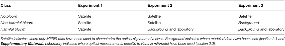
Table 1. Summary of combination of training datasets for the simulation experiments.

2.3.1. Training Datasets

The training dataset in Experiment 1 was taken as the reference. It was generated from MERIS sensor measurements of R_rs at wavelengths 413, 443, 490, 510, 560, 620, 665, 681, and 709 nm. Absorption and backscattering coefficients derived from inversion algorithms (e.g., Smyth et al., 2007) were not used in this training dataset. Using IOP derived from MERIS data introduced additional uncertainty (Defoin-Platel and Chami, 2007; Werdell et al., 2018). Historical MERIS scenes with documented K. mikimotoi bloom events in the English Channel in years 2002–2004, were selected (Kelly-Gerreyn et al., 2004; Vanhoutte-Brunier et al., 2008). Areas of these scenes were manually delineated and labeled into no bloom, non-harmful, and harmful classes. In total five MERIS scenes were selected on 19 July 2002, 1 and 7 July 2003, 10 and 23 July 2004. To compose a training dataset the images were first sub-sampled by a factor of 4. Overall, 6.25% of satellite pixels were used for training and 93.75% were used for evaluation (section 2.3.2). The data in the training dataset were arranged in a 2D table format with R_rs values and class labels of individual image pixels stored in rows. In total the training table contained 14,072 records of no bloom class, 12,116 records of non-harmful bloom class, and 10,294 records of harmful bloom class.

In Experiment 2, the records in the training table labeled as harmful bloom were removed. R_rs spectra harmful bloom class results from the addition of the background optical properties from bio-optical models (section 2.1) to the K. mikimotoi optical properties derived from laboratory experiments (section 2.2), to include in the training dataset the effect of a mixed particle assemblage in a HAB event. Values used for TChla_km varied from 1 to 15 mgm⁻³ with a constant step in logarithm scale resulting in 500 concentrations. TChla_bg varied from 0.01 to 2 mgm⁻³ having 10 concentrations with an identical interval in logarithm scale, therefore a total of 5,000 combinations were obtained.

Experiment 3, was the same as Experiment 2 but with the non-harmful bloom class defined by the background optical properties from bio-optical models (section 2.1), with TChla_bg between 1 and 10 mgm⁻³. From each experiment, a set of classifier coefficients was obtained after training. In all the Experiments, the no bloom class was defined using the manual selection of parts of the satellite images.

2.3.2. Evaluation Dataset

Due to lack of in situ data to perform an independent validation of the classification, the results from each Experiment were evaluated with the part of the training images that had been reserved (i.e., not used for training). The performance was quantified through statistical comparisons with the manually classified pixels. The same 5 MERIS scenes as those used for training were used to generate training and evaluation datasets for the HAB classifier (see section 2.3.1). The same evaluation dataset was applied in all three experiments, but the classification results were different because the training data were different.

The measures of performance included a confusion matrix and derived statistical measures: overall accuracy, kappa coefficient, errors of commission, and producer accuracy. Overall accuracy was calculated as the number of correctly classified pixels divided by the total number of classified pixels. The kappa coefficient measures the agreement between the evaluation dataset and the classification results in the range from 0 to 1. The data can be considered to be in perfect statistical agreement when kappa is 1 and disagree when kappa equals 0. Errors of commission is the measure of false positive, estimated for each class as the fraction of pixels that were classified incorrectly. Producer accuracy is calculated for each class as the probability that the pixels in this class were classified correctly.

Not all of the classified image pixels were used for estimation of the confusion matrix. If the probability of unknown class was higher than 0.6 or the probability of any of other three classes was lower that 0.6, the pixel was considered as unreliable and discarded.

3. Results and Discussion

3.1. Optical Properties: Modeled Data for Background and Laboratory Experiments for Karenia mikimotoi

The background model is constructed with the underlying hypothesis that at lower TChl_bg, the smaller phytoplankton sizes dominate the optical properties. For absorption (Figure 1A) this means that there is a higher slope for lower chlorophyll concentrations (i.e., less than ~2 mg Chla m⁻³). Larger cells are expected to have lower per-chlorophyll absorption due to the package effect (Bricaud et al., 2004). Values from this laboratory experiment are greater than those predicted by the model, pointing toward higher TChla per cell in the culture. However, the values are close to other studies for HAB-forming dinoflagellates (Cannizzaro et al., 2008).

FIGURE 1

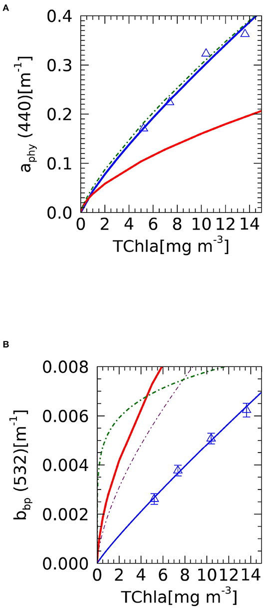
Figure 1. Relationship between measured TChla and optical properties at a given wavelength. Red solid line is the background model and blue solid triangles and line are experimental results from this study for Karenia mikimotoi: (A) Phytoplankton absorption. Green dot-dash line are Cannizzaro et al. (2008) predictions of a_phy(443) for >10⁻⁴ cells l⁻¹; (B) b_bp,km(532). Green dotted-dash line are Cannizzaro et al. (2008) predictions of b_bp(532) for >10⁻⁴ cells l⁻¹; purple alternate-dash is Antoine et al. (2011). Symbols are median experimental values and error bars are IQR. Solid lines are power law fit to these data (Table 2).

The backscattering coefficient is also modeled as a power law for the background (Figure 1B), following the same underlying assumption of smaller cells dominating optical properties of lower chlorophyll concentrations (Loisel and Morel, 1998). Measurements from the current laboratory experiment are lower than those predicted by the background model, but similar to other laboratory experiments. For example, $b_{bp,km}^{*}(470)$ = 0.000525 m⁻² mg Chla⁻¹ is comparable to the lower values obtained for other species of dinophyceae ($b_{bp}^{*}(442)$ from 0.0005786 to 0.0009194 m⁻² mg Chla⁻¹ ) (Whitmire et al., 2010). These laboratory values are low in comparison with other field studies in coastal waters (Antoine et al., 2011) and in areas with HAB blooms (Cannizzaro et al., 2008). This disagreement is to be expected, as the in situ studies incorporate the b_bp signal from the whole population, which is an assemblage of phytoplankton and other particles (Stramski et al., 2001; Martinez-Vicente et al., 2010, 2012). In fact, for Experiment 2, the harmful class b_bp(532) can vary from 0.00718 m⁻¹ for 1.01 mg Chla m⁻³ to 0.01112 m⁻¹ for 17 mg Chla m⁻³, when the contributions of background and K. mikimotoi were added. As a comparison, Cannizzaro et al. (2008) predicts b_bp(532) = 0.00855 m⁻¹ for 17 mg Chla m⁻³. The coefficients resulting from the power law fit to the laboratory data, used by the classifier, are summarized in Table 2.

TABLE 2

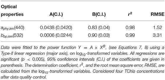
Table 2. Regression coefficients and statistics of the fit for a_phy,km(440) and b_bp,km(532), as a function of chlorophyll concentration, TChla.

The second set of parameters needed in Equations (7) and (8) are the chlorophyll-specific spectrally varying inherent optical properties (Supplementary Figure 1). For chlorophyll-specific absorption, the model predicts a flattening of the spectra at higher chlorophyll concentrations. The median values obtained from the laboratory experiment are consistent with this prediction for the blue part of the spectra (400–500 nm) but they are higher for the red. However, the experiment is in close agreement with previous laboratory experiments, in particular with observations under low light conditions (see Figure 4 in Stæhr and Cullen, 2003). Concerning the spectral chlorophyll-specific backscattering coefficient (Supplementary Figure 1), modeled values for the background follow also the assumption of smaller phytoplankton sizes dominating at lower TChl_bg. This leads to higher chlorophyll-specific backscattering values (i.e., smaller phytoplankton is more efficient at backscattering light) and more features due to absorption effects on the backscattering spectral shape.

Backscattering ratio (Figure 2) shows that the laboratory measurements are 6% higher than other experimental data from the literature specific to the same species (Harmel et al., 2016), and within range for other dinophyceae algae [${\tilde{b}}_{bp}(442)$ from 0.0061 to 0.0210] (Whitmire et al., 2010). The laboratory experiment results also aligns with in situ observations (Whitmire et al., 2007; Cannizzaro et al., 2008).

FIGURE 2

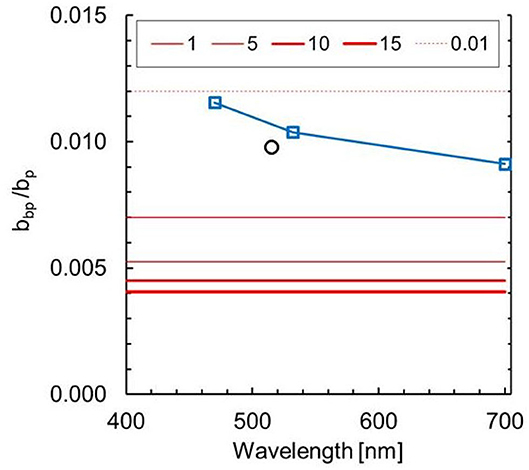
Figure 2. Spectral backscattering ratio (${\tilde{b}}_{bp}$= b_bp/b_p) for background model and for Karenia mikimotoi from laboratory. Red lines are modeled values at different TChla. Blue squares and line are median values from experimental data. Black circle is value reported by Harmel et al. (2016).

3.2. Training Dataset From Modeled and Laboratory Data

The forward calculated R_rs from background and laboratory experiments are shown in Figure 3, for different chlorophyll concentrations, alongside the training dataset derived from pixels in the satellite image manual selection. The no bloom class is defined in all Experiments from the manual selection in the satellite image. Figures 3B,D display the results for the background model reflectances. Increase in TChla controls the shape of the spectra. These data are used for training class non-harmful bloom and harmful bloom (Table 1). Figure 3F shows modeled R_rs spectra for K. mikimotoi using the specific optical properties derived from the laboratory experiments.

FIGURE 3

Figure 3. R_rs spectra used for training the HAB classifier. (A,C,E) Median and standard deviation R_rs from MERIS pixels for no bloom, no harmful, and harmful classes, respectively (section 2.3). (B,D,F) R_rs spectra at different TChla concentrations for background (B,D) and Karenia mikimotoi (F) datasets used to train the classifier in Experiments 2 and 3. MERIS bands are indicated by stars.

The median R_rs spectrum for the no bloom class from satellite (Figure 3A) compares well in magnitude and shape to R_rs modeled for the lower TChl_bg (Figure 3B). Median TChla for no bloom from satellite, computed using OC5, is 0.35 mg Chla m⁻³ and dispersion (half the inter-decile range = (Q90-Q10)/2) is 0.13 mg Chla m⁻³. The harmful class from satellite (Figure 3E) and from the laboratory experiments (Figure 3F) are also in agreement of scale and spectral shape. TChla from the satellite is 8.15 ± 10.6 mg Chla m⁻³, which encompasses the range of TChla_km simulated. However, R_rs spectra of the harmless bloom class from satellite (Figure 3C) is lower than the R_rs modeled (Figure 3D). Satellite TChla is 1.01 ± 0.52 mg Chla m⁻³ and is representative of the lower limit of the simulated range (i.e., from 1 mg Chla m⁻³) for the background, which could explain some differences in the results below. The classifier coefficients are available and attached to this paper (Supplementary Material, section 3).

3.3. Detection of HABs in Satellite Data

Figure 4 presents two examples of MERIS scenes with documented K. mikimotoi blooms. These scenes were selected to train and to compare the sensitivity of the classifier to training datasets in Experiments 1, 2, and 3 (see section 2.3). The enhanced MERIS true color images of the bloom are shown in Figures 4A,B. The harmful bloom class can be seen in the images as a reddish patch close to the center of the images. Figures 4C,D show the TChla as retrieved by standard chlorophyll algorithm for the area, highlighting the co-location of elevated TChla with harmful bloom class. The manual delineation of the area around those blooms for harmful bloom is shown in red in Figures 4E,F.

FIGURE 4

Figure 4. MERIS images showing a Karenia mikimotoi bloom in the English Channel on 19 July 2002 (A,C,E) and 1 July 2003 (B,D,F). Enhanced true colour images (A,B) and chlorophyll concentration from Algorithm OC5 for MERIS (C,D) (Tilstone et al., 2017). Image masks used for training and evaluation of Karenia mikimotoi HAB classifier (E,F). Blue areas indicate data selected to construct the training dataset for no bloom class. Green areas are for non-harmful bloom training dataset. Red areas for a generic harmful bloom class training dataset.

The turquoise and darker greenish colors, mostly toward the Atlantic Ocean, are associated with no bloom and non-harmful bloom classes (Figures 4A,B). They match low to medium TChla (Figures 4C,D). The manually selected areas for these classes are blue and green respectively (Figures 4E,F). In these examples, the pixels manually selected for the non-harmful bloom class are mostly toward the Atlantic Ocean, with TChla~1 mgm⁻³, which explains the R_rs (Figure 3C). A special case is the white bright patch on the Western English Channel, close to the coast of England (Figure 4A). This corresponds to a bloom of non-toxic coccolithophores species, which has not been identified as high TChla (Figure 4C) and has not been labeled as a separate class in the classifier. However, the chlorophyll algorithm is not always capable to discern “bright” waters from high chlorophyll concentrations. For instance, toward the North, in the Bristol Channel, an orangy-white patch, is a well documented location of high riverine contributions of suspended particulate matter (Neil et al., 2011) (Figures 4A,B). Finally, at the center of the Western English Channel, dark red patches (Figures 4A,B) match the corresponding extremely high chlorophyll concentration images (Figures 4C,D) from documented blooms (Kelly-Gerreyn et al., 2004; Vanhoutte-Brunier et al., 2008). These patches were used to define the harmful bloom class manually from satellite (Figures 4E,F). are distinguishable. Overall, high TChla can be considered a good indicator of areas with potential HAB, however, highly turbid waters in coastal areas can produce misleading high TChla when chlorophyll algorithms fail. Lack of in situ data to verify high-chlorophyll non-harmful bloom areas, preclude drawing any conclusion about the validity of using the current algorithm and training datasets to identify those, and it is an extension for this study.

The scenes in Figure 4 were further processed using the K. mikimotoi classifier, trained with the datasets in Experiments 1–3 to generate risk maps (Figure 5). Qualitatively, the three experiments produced overall similar maps with some interesting localized differences (Figure 5). The classification results were different in the Bristol Channel, where concentration of sediments was relatively high. No collocated in situ suspended particulate matter are available, but this is well known area of intense bottom resuspension of sediments and river runoff (Uncles, 2010; Uncles et al., 2015). In Experiment 1 (Figures 5A,B) the classifier, trained on satellite data, discriminated this region as HAB. This false positive detection disappeared in Experiments 2 and 3 (Figures 5C–F), highlighting an improvement of performance in this optically complex region. Another observation in these examples is that the coverage by grey areas increased from Experiments 1 to 3. Indeed, the percentage of unknown class pixels (Table 3) shows a slight increase from Experiment 1 to Experiment 2. It has the highest value for Experiment 3, indicating where the algorithm fails to classify a pixel among one of the known categories. Figures 5E,F point to greater areas of grey (unknown class) coinciding with areas of lower TChla (Figures 4C,D). The increase in unknown class for Experiment 3 can be related to using a range of chlorophyll for modeling the non-harmful class with higher values than what is normally encountered in the area (i.e., ~1.5 mg Chla m⁻³ from Smyth et al., 2010). It is worth noting that the coccolithophore bloom was classified as unknown in Figures 5A,C,E for the three Experiments. None of the satellite training images or simulated data for the three training classes included the coccolithophore bloom examples and in all three experiments the algorithm correctly discriminated these data as unknown class.

FIGURE 5

Figure 5. Karenia mikimotoi HAB classification maps of the English Channel on 19 July 2002 (left column) and 1 July 2003 (right column): (A,B) Experiment 1, (C,D) Experiment 2, and (E,F) Experiment 3. Pixels classified as Harmful bloom are shown in red, non-harmful bloom in green, and no bloom in blue. Pixels classified as unknown, are presented in gray and black is land within contours and missing data over water, due to cloud cover or sun glint.

TABLE 3

Table 3. The percentage of image pixels, classified as unknown.

Numerically, the comparisons of the classification algorithm was assessed using the confusion matrix and statistical measures derived from the confusion matrix. The results of classifier assessment in Experiments 1–3 are summarized in Tables 4, 5. Due to the limited availability of in situ data for validation, the evaluation of the experiments has been made using satellite data (see section 2.3), the focus being on the relative changes in the results.

TABLE 4

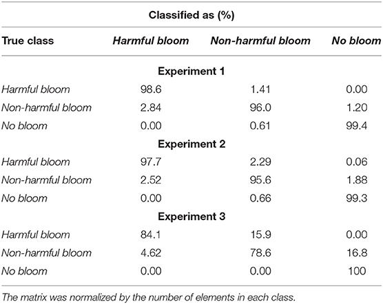
Table 4. The confusion matrix for Karenia mikimotoi classifier.

TABLE 5

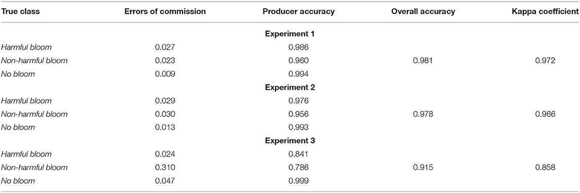
Table 5. Performance measures derived from the confusion matrix.

Overall, there are small differences among the results from the Experiments. Importantly, Experiment 1 and 2 percentage classification of harmful bloom class is <1% and the greatest difference is <15% (Table 4). The confusion matrix demonstrates that the accuracy of non-harmful bloom classification is lower for the Experiment 3. The differences in results between Experiment 1 and 3 may be due to the difference in the range of R_rs for the ranges of TChla considered for the non-harmful bloom class, as discussed above. The small differences between Experiment 1 and 2 may point to expected variability of the optical properties within the K. mikimotoi culture. It follows from Table 4 that the classifier results in Experiment 2 have the lowest false positive rate for non-harmful blooms being classified as K. mikimotoi (i.e., 2.52). This observation is in good agreement with the classified maps in Figure 5 that showed reduced false alarms in the Bristol Channel for Experiment 2 and even fewer in Experiment 3.

According to the results, all three classifiers performed well, achieving overall accuracy above 0.91 and kappa value above 0.85 (Table 5). The best performance was demonstrated by the classifier in Experiment 1 and the worst for the classifier in Experiment 3 with 7% lower overall accuracy, highlighting the importance of the choice of ranges in chlorophyll adapted to the region of study. However, the fact that the difference among using different training datasets was low (i.e., subjective in Experiment 1 vs. laboratory-derived in Experiment 2), supports the use of laboratory data to train this type of classifier.

The errors of commission and producer accuracy statistical measures for different classes are summarized in Table 5. These values are quite similar for Experiment 1 and Experiment 2, indicating that the performance loss is relatively small when the satellite training data for harmful bloom are replaced with laboratory derived data in Experiment 2. This points to a small degradation of the classification accuracy using laboratory data. A more significant loss in accuracy can be observed in Experiment 3, where the producer accuracy for non-harmful bloom class is reduced by almost 20% by using the bio-optical model instead of satellite-derived data for training.

Overall, the results demonstrate that the novel approach based on laboratory experiments can be used for simulation of R_rs values and training of a HAB classifier with only slight degradation of the classification accuracy while reducing false positives due to turbid coastal waters. This study has highlighted the impact of the selection ranges for no bloom conditions that should be fit to simulate TChla similar to those found in the environment where the model is deployed. A smaller source of uncertainty could be related to the use of laboratory conditions as representative of natural conditions for K. mikimotoi. A wider set of culture conditions of the phytoplankton could allow for increasing the training dataset to be able to deal with the natural environmental variability to which the phytoplankton is exposed in the real ocean. We speculate that the low light culture conditions in our experiment could have affected the optical properties of the phytoplankton. While they are in agreement with other studies under similar conditions (Whitmire et al., 2010; Harmel et al., 2016), the variability with light intensity and adaptation should be considered and included in subsequent training datasets (Poulin et al., 2018). More complex modeling of R_rs by different mixes of phytoplankton species and use of more advanced radiative transfer modeling (Mobley and Stramski, 1997; Stramski and Mobley, 1997) could also make our training dataset more robust. However, it is the lack of in situ observations co-incident with either radiometry from in situ and/or satellite platforms that limits further advance (Tomlinson et al., 2009), as we were unable to validate our results against real-world observations. Therefore, more efforts to collate existing data and to gather new ones are required.

4. Conclusions and Further Work

In this work, a novel approach, tested through a sensitivity study, to produce training datasets for HAB classification using machine learning methods has been proposed. The novelty of the approach consists in injecting the bio-optical knowledge from the literature and from a purpose built laboratory experiment into a training dataset for detection of a specific phytoplankton species that can cause health and economic harm to the coastal communities.

The potential advantages of this approach include moving away from subjectivity in terms of selection of training datasets as well as not being sensor or even region specific. It is easy to envisage that this approach can be applied to radiometric sensors installed in multiple platforms such as ferries, drones or different satellites.

Laboratory measurements of absorption and backscattering coefficients for different concentrations of K. mikimotoi chlorophyll have been performed, matching existing observations at low light conditions of the culture. When these data were used to train a HABs classifier and applied to MERIS images from the European coastal shelf, there was <1% degradation of the capacity to detect the harmful bloom in comparison to using satellite data, but there was a better discrimination of false positives in turbid coastal waters. Further tests on the ability to separate non-harmful from harmful algal blooms when both have high chlorophyll concentrations are needed. Even replacing most of the training datasets with a combination of modeled and laboratory derived R_rs did not degrade HAB detection significantly, although regional average chlorophyll concentrations need to be known a priory to improve the results.

The limited availability of suitable datasets to ground truth the results, constrains the conclusions of this study to a sensitivity analysis. If HAB detection from satellite is to progress to become an operational satellite product, in a similar way radiometry or Chla products are, the construction and open availability of standardized and purpose built relevant validation datasets should be the focus of future work. Indeed, when in situ observations are available (Caballero et al., 2020), local tuning of an algorithm can be achieved. The approach proposed here could be ported to different species by modifying the training datasets.

Data Availability Statement

The datasets presented in this study can be found in online repositories. The names of the repository/repositories and accession number(s) can be found at: https://doi.org/10.5281/zenodo.4075095.

Author Contributions

VM-V designed the experiment, carried out the experiment, and wrote the first draft of the manuscript. VB, CS, AA, and VV helped out with the experiment in the laboratory. AK and JL did the numerical experiments. PM discussed initial ideas. All co-authors provided comments to the manuscript.

Funding

This work benefited from funding from EC-FP7 AQUA-USERS (Grant 607325), Interreg Atlantic Area project PRIMROSE (Grant EAPA 182/2016), NERC ShellEye (Grant NE/P011004/1), Fundação para a Ciência e Tecnologia through the strategic project UIDB/04292/2020. This work was also supported by funding from the European Union's Horizon 2020 Research and Innovation Programme under grant agreement N 810139: Project Portugal Twinning for Innovation and Excellence in Marine Science and Earth Observation—PORTWIMS. Also supported by HABWAVE project LISBOA-01-0145-FEDER-031265, co-funded by EU ERDF funds, within the PT2020 Partnership Agreement and Compete 2020, and national funds through FCT, I.P.

Conflict of Interest

The authors declare that the research was conducted in the absence of any commercial or financial relationships that could be construed as a potential conflict of interest.

Acknowledgments

Thanks to C. Beltran for the analysis of HPLC samples and G.Dall'Olmo for initial advice on the setup of the optical chamber. We acknowledge the comments and suggestions from three reviewers who have contributed to improve this work.

Supplementary Material

The Supplementary Material for this article can be found online at: https://www.frontiersin.org/articles/10.3389/fmars.2020.582960/full#supplementary-material

References

Ahn, Y. H., Bricaud, A., and Morel, A. (1992). Light backscattering efficiency and related properties of some phytoplankters. Deep-Sea Res. Part A Oceanogr. Res. Pap. 39, 1835–1855. doi: 10.1016/0198-0149(92)90002-B

CrossRef Full Text | Google Scholar

Andersen, R. A. (2005). Algal Culturing Techniques. London: Elsevier.

Google Scholar

Antoine, D., Siegel, D. A., Kostadinov, T. S., Maritorena, S., Nelson, N. B., Gentili, B., et al. (2011). Variability in optical particle backscattering in contrasting bio-optical oceanic regimes. Limnol. Oceanogr. 56, 955–973. doi: 10.4319/lo.2011.56.3.0955

CrossRef Full Text | Google Scholar

Babin, M., Roesler, C., and Cullen, J. J. (2008). Real-Time Coastal Observing Systems for Marine Ecosystem Dynamics and Harmful Algal Blooms. Oceanographic Methodology Series. Paris: UNESCO.

Google Scholar

Barnes, M. K., Tilstone, G. H., Smyth, T. J., Widdicombe, C. E., Gloël, J., Robinson, C., et al. (2015). Drivers and effects of Karenia mikimotoi blooms in the western English channel. Prog. Oceanogr. 137, 456–469. doi: 10.1016/j.pocean.2015.04.018

CrossRef Full Text | Google Scholar

Bricaud, A., Bedhomme, A. L., and Morel, A. (1988). Optical-properties of diverse phytoplanktonic species - experimental results and theoretical interpretation. J. Plankt. Res. 10, 851–873. doi: 10.1093/plankt/10.5.851

CrossRef Full Text | Google Scholar

Bricaud, A., Claustre, H., Ras, J., and Oubelkheir, K. (2004). Natural variability of phytoplanktonic absorption in oceanic waters: influence of the size structure of algal populations. J. Geophys. Res. 109:C11010. doi: 10.1029/2004JC002419

CrossRef Full Text | Google Scholar

Bricaud, A., Morel, A., Babin, M., Allali, K., and Claustre, H. (1998). Variations of light absorption by suspended particles with chlorophyll a concentration in oceanic (case 1) waters: analysis and implications for bio-optical models. J. Geophys. Res. 103, 31033–31044. doi: 10.1029/98JC02712

CrossRef Full Text | Google Scholar

Bricaud, A., Morel, A., and Prieur, L. (1983). Optical-efficiency factors of some phytoplankters. Limnol. Oceanogr. 28, 816–832. doi: 10.4319/lo.1983.28.5.0816

CrossRef Full Text | Google Scholar

Browning, T. J., Stone, K., Bouman, H. A., Mather, T. A., Pyle, D. M., Moore, C. M., et al. (2015). Volcanic ash supply to the surface ocean?remote sensing of biological responses and their wider biogeochemical significance. Front. Mar. Sci. 2:14. doi: 10.3389/fmars.2015.00014

CrossRef Full Text | Google Scholar

Caballero, I., Fernández, R., Escalante, O. M., Mamán, L., and Navarro, G. (2020). New capabilities of sentinel-2a/b satellites combined with in situ data for monitoring small harmful algal blooms in complex coastal waters. Sci. Rep. 10:8743. doi: 10.1038/s41598-020-65600-1

PubMed Abstract | CrossRef Full Text | Google Scholar

Cannizzaro, J. P., Carder, K. L., Chen, F. R., Heil, C. A., and Vargo, G. A. (2008). A novel technique for detection of the toxic dinoflagellate, karenia brevis, in the Gulf of Mexico from remotely sensed ocean color data. Contin. Shelf Res. 28, 137–158. doi: 10.1016/j.csr.2004.04.007

CrossRef Full Text | Google Scholar

Cullen, J. J., Ciotti, u. M., Davis, R. F., and Lewis, M. R. (1997). Optical detection and assessment of algal blooms. Limnol. Oceanogr. 42(5 Part 2), 1223–1239. doi: 10.4319/lo.1997.42.5_part_2.1223

CrossRef Full Text | Google Scholar

Defoin-Platel, M., and Chami, M. (2007). How ambiguous is the inverse problem of ocean color in coastal waters? J. Geophys. Res. 112, 1–16. doi: 10.1029/2006JC003847

CrossRef Full Text | Google Scholar

Dierssen, H., McManus, G. B., Chlus, A., Qiu, D., Gao, B.-C., and Lin, S. (2015). Space station image captures a red tide ciliate bloom at high spectral and spatial resolution. Proc. Natl. Acad. Sci. U.S.A. 112, 14783–14787. doi: 10.1073/pnas.1512538112

PubMed Abstract | CrossRef Full Text | Google Scholar

Finkel, Z., and Irwin, A. (2001). Light absorption by phytoplankton and the filter amplification correction: cell size and species effects. J. Exp. Mar. Biol. Ecol. 259, 51–61. doi: 10.1016/S0022-0981(01)00225-8

PubMed Abstract | CrossRef Full Text | Google Scholar

Gordon, H. R., Brown, O. B., Evans, R. H., Brown, J. W., Smith, R. C., Baker, K. S., et al. (1988). A semianalytic radiance model of ocean color. J. Geophys. Res. 93, 10909–10924. doi: 10.1029/JD093iD09p10909

CrossRef Full Text | Google Scholar

Griffith, A. W., and Gobler, C. J. (2020). Harmful algal blooms: A climate change co-stressor in marine and freshwater ecosystems. Harmf. Algae 91:101590. doi: 10.1016/j.hal.2019.03.008

PubMed Abstract | CrossRef Full Text | Google Scholar

Harmel, T., Hieronymi, M., Slade, W., Rottgers, R., Roullier, F., and Chami, M. (2016). Laboratory experiments for inter-comparison of three volume scattering meters to measure angular scattering properties of hydrosols. Opt. Exp. 24, A234–A256. doi: 10.1364/OE.24.00A234

PubMed Abstract | CrossRef Full Text | Google Scholar

Kelly-Gerreyn, B., Qurban, M., Hydes, D., Miller, P., and Fernand, L. (2004). “Coupled ferrybox ship of opportunity and satellite data observations of plankton succession across the European shelf sea and Atlantic Ocean,” in International Council for the Exploration of the Sea (ICES) Annual Science Conference, Vigo.

Google Scholar

Kudela, R. M., Berdelet, E., Bernard, S., Burford, M., Fernand, L., Lu, S., et al. (2015). Harmful Algal Blooms. A Scientific Summary for Policy Makers. Paris: IOC/UNESCO, (IOC/INF-1320).

Google Scholar

Kurekin, A., Miller, P. I., and Van der Woerd, H. J. (2014). Satellite discrimination of Karenia mikimotoi and phaeocystis harmful algal blooms in European coastal waters: Merged classification of ocean colour data. Harmf. Algae 31, 163–176. doi: 10.1016/j.hal.2013.11.003

PubMed Abstract | CrossRef Full Text | Google Scholar

Loisel, H., and Morel, A. (1998). Light scattering and chlorophyll concentration in case 1 waters: a reexamination. Limnol. Oceanogr. 43, 847–858. doi: 10.4319/lo.1998.43.5.0847

CrossRef Full Text | Google Scholar

Martinez-Vicente, V., Land, P. E., Tilstone, G. H., Widdicombe, C., and Fishwick, J. R. (2010). Particulate scattering and backscattering related to water constituents and seasonal changes in the western English channel. J. Plankton Res. 32, 603–619. doi: 10.1093/plankt/fbq013

CrossRef Full Text | Google Scholar

Martinez-Vicente, V., Tilstone, G. H., Sathyendranath, S., Miller, P. I., and Groom, S. B. (2012). Contributions of phytoplankton and bacteria to the optical backscattering coefficient over the mid-Atlantic ridge. Mar. Ecol. Prog. Ser. 445, 37–51. doi: 10.3354/meps09388

CrossRef Full Text | Google Scholar

Mendes, C. R., Cartaxana, P., and Brotas, V. (2007). HPLC determination of phytoplankton and microphytobenthos pigments: comparing resolution and sensitivity of a C18 and a C8 method. Limnol. Oceanogr. 5, 363–370. doi: 10.4319/lom.2007.5.363

CrossRef Full Text | Google Scholar

Miller, P. I., Shutler, J. D., Moore, G. F., and Groom, S. B. (2006). Seawifs discrimination of harmful algal bloom evolution. Int. J. Rem. Sens. 27, 2287–2301. doi: 10.1080/01431160500396816

CrossRef Full Text | Google Scholar

Millie, D. F., Schofield, O. M., Kirkpatrick, G. J., Johnsen, G., Tester, P. A., and Vinyard, B. T. (1997). Detection of harmful algal blooms using photopigments and absorption signatures: a case study of the florida red tide dinoflagellate, gymnodinium breve. Limnol. Oceanogr. 42(5 Part 2), 1240–1251. doi: 10.4319/lo.1997.42.5_part_2.1240

CrossRef Full Text | Google Scholar

Millie, F, D., Kirkpatrick, J, G., and Vinyard, T, B. (1995). Relating photosynthetic pigments and in vivo optical density spectra to irradiance for the florida red-tide dinoflagellate gymnodinium breve. Mar. Ecol. Prog. Ser. 120, 65–75. doi: 10.3354/meps120065

CrossRef Full Text | Google Scholar

Mobley, C., and Sundman, L. (2016). HydroLight 5.3.0- EcoLight 5.3.0 Technical Documentation. Sequoia Inc.

Google Scholar

Mobley, C. D., and Stramski, D. (1997). Effects of microbial particles on oceanic optics: methodology for radiative transfer modeling and example simulations. Limnol. Oceanogr. 42, 550–560. doi: 10.4319/lo.1997.42.3.0550

CrossRef Full Text | Google Scholar

Neil, C., Cunningham, A., and McKee, D. (2011). Relationships between suspended mineral concentrations and red-waveband reflectances in moderately turbid shelf seas. Rem. Sens. Environ. 115, 3719–3730. doi: 10.1016/j.rse.2011.09.010

CrossRef Full Text | Google Scholar

Pope, R., and Fry, E. (1997). Absorption spectrum (380-700 nm) of pure water. II. integrating cavity measurements. Appl. Opt. 36, 8710–8723. doi: 10.1364/AO.36.008710

PubMed Abstract | CrossRef Full Text | Google Scholar

Poulin, C., Antoine, D., and Huot, Y. (2018). Diurnal variations of the optical properties of phytoplankton in a laboratory experiment and their implication for using inherent optical properties to measure biomass. Opt. Exp. 26, 711–729. doi: 10.1364/OE.26.000711

PubMed Abstract | CrossRef Full Text | Google Scholar

Sanseverino, I., Conduto, D., Pozzoli, L., Dobricic, S., and Lettieri, T. (2016). Algal Bloom and Its Economic Impact. Number EUR 27905 EN. Library Catalog: ec.europa.eu.

Google Scholar

Shang, S., Wu, J., Huang, B., Lin, G., Lee, Z., Liu, J., et al. (2014). A new approach to discriminate dinoflagellate from diatom blooms from space in the East China Sea. J. Geophys. Res. 119, 4653–4668. doi: 10.1002/2014JC009876

CrossRef Full Text | Google Scholar

Slade, W. H., Boss, E., Dall'Olmo, G., Langner, M. R., Loftin, J., Behrenfeld, M. J., et al. (2010). Underway and moored methods for improving accuracy in measurement of spectral particulate absorption and attenuation. J. Atmos. Ocean. Technol. 27, 1733–1746. doi: 10.1175/2010JTECHO755.1

CrossRef Full Text | Google Scholar

Smyth, T. J., Fishwick, J. R., AL-Moosawi, L., Cummings, D. G., Harris, C., Kitidis, V., et al. (2010). A broad spatio-temporal view of the western English channel observatory. J. Plankton Res. 32, 585–601. doi: 10.1093/plankt/fbp128

CrossRef Full Text | Google Scholar

Smyth, T. J., Moore, G. F., Hirata, T., and Aiken, J. (2007). Semianalytical model for the derivation of ocean color inherent optical properties: description, implementation, and performance assessment: erratum. Appl. Opt. 46, 429–430. doi: 10.1364/AO.46.000429

CrossRef Full Text | Google Scholar

Stæhr, P. A., and Cullen, J. J. (2003). Detection of Karenia mikimotoi by spectral absorption signatures. J. Plankton Res. 25, 1237–1249. doi: 10.1093/plankt/fbg083

CrossRef Full Text | Google Scholar

Stramski, D., Bricaud, A., and Morel, A. (2001). Modeling the inherent optical properties of the ocean based on the detailed composition of the planktonic community. Appl. Opt. 40, 2929–2945. doi: 10.1364/AO.40.002929

PubMed Abstract | CrossRef Full Text | Google Scholar

Stramski, D., and Mobley, C. D. (1997). Effects of microbial particles on oceanic optics: a database of single-particle optical properties. Limnol. Oceanogr. 42, 538–549. doi: 10.4319/lo.1997.42.3.0538

CrossRef Full Text | Google Scholar

Stramski, D., and Morel, A. (1990). Optical properties of photosynthetic picoplankton in different physiological states as affected by growth irradiance. Deep Sea Res. Part A Oceanogr. Res. Pap. 37, 245–266. doi: 10.1016/0198-0149(90)90126-G

CrossRef Full Text | Google Scholar

Tassan, S., and Ferrari, G. M. (1995). An alternative approach to absorption measurements of aquatic particles retained on filters. Limnol. Oceanogr. 40, 1358–1368. doi: 10.4319/lo.1995.40.8.1358

CrossRef Full Text | Google Scholar

Tilstone, G., Mallor-Hoya, S., Gohin, F., Couto, A. B., Sá, C., Goela, P., et al. (2017). Which ocean colour algorithm for MERIS in North West European waters? Rem. Sens. Environ. 189, 132–151. doi: 10.1016/j.rse.2016.11.012

CrossRef Full Text | Google Scholar

Tomlinson, M. C., Wynne, T. T., and Stumpf, R. P. (2009). An evaluation of remote sensing techniques for enhanced detection of the toxic dinoflagellate, Karenia Brevis. Rem. Sens. Environ. 113, 598–609. doi: 10.1016/j.rse.2008.11.003

CrossRef Full Text | Google Scholar

Uncles, R. J. (2010). Physical properties and processes in the Bristol channel and Severn estuary. Mar. Pollut. Bull. 61, 5–20. doi: 10.1016/j.marpolbul.2009.12.010

PubMed Abstract | CrossRef Full Text | Google Scholar

Uncles, R. J., Stephens, J. A., and Harris, C. (2015). Estuaries of southwest England: salinity, suspended particulate matter, loss-on-ignition and morphology. Prog. Oceanogr. 137, 385–408. doi: 10.1016/j.pocean.2015.04.030

CrossRef Full Text | Google Scholar

Vaillancourt, R. D., Brown, C. W., Guillard, R. R. L., and Balch, W. M. (2004). Light backscattering properties of marine phytoplankton: relationships to cell size, chemical composition and taxonomy. J. Plankton Res. 26, 191–212. doi: 10.1093/plankt/fbh012

CrossRef Full Text | Google Scholar

Vanhoutte-Brunier, A., Fernand, L., Ménesguen, A., Lyons, S., Gohin, F., and Cugier, P. (2008). Modelling the Karenia mikimotoi bloom that occurred in the western English channel during summer 2003. Ecol. Model. 210, 351–376. doi: 10.1016/j.ecolmodel.2007.08.025

CrossRef Full Text | Google Scholar

Weihs, C., Ligges, U., Luebke, K., and Raabe, N. (2005). “KLAR analyzing German business cycles,” in Data Analysis and Decision Support, eds D. Baier, R. Decker, and L. Schmidt-Thieme (Berlin: Springer-Verlag), 335–343. doi: 10.1007/3-540-28397-8_36

CrossRef Full Text | Google Scholar

Werdell, P. J., McKinna, L. I. W., Boss, E., Ackleson, S. G., Craig, S. E., Gregg, W. W., et al. (2018). An overview of approaches and challenges for retrieving marine inherent optical properties from ocean color remote sensing. Prog. Oceanogr. 160, 186–212. doi: 10.1016/j.pocean.2018.01.001

PubMed Abstract | CrossRef Full Text | Google Scholar

Wetlabs (2009). Ac-Meter Protocol Revision p. Technical report.

Whitmire, A. L., Boss, E., Cowles, T. J., and Pegau, W. S. (2007). Spectral variability of the particulate backscattering ratio. Opt. Exp. 15, 7019–7031. doi: 10.1364/OE.15.007019

PubMed Abstract | CrossRef Full Text | Google Scholar

Whitmire, A. L., Pegau, W. S., Karp-Boss, L., Boss, E., and Cowles, T. J. (2010). Spectral backscattering properties of marine phytoplankton cultures. Opt. Exp. 18, 15073–15093. doi: 10.1364/OE.18.015073

PubMed Abstract | CrossRef Full Text | Google Scholar

Xi, H., Hieronymi, M., Krasemann, H., and Röttgers, R. (2017). Phytoplankton group identification using simulated and in situ hyperspectral remote sensing reflectance. Front. Mar. Sci. 4:272. doi: 10.3389/fmars.2017.00272

CrossRef Full Text | Google Scholar

Xi, H., Hieronymi, M., Röttgers, R., Krasemann, H., and Qiu, Z. (2015). Hyperspectral differentiation of phytoplankton taxonomic groups: a comparison between using remote sensing reflectance and absorption spectra. Remote Sens. 7:14781. doi: 10.3390/rs71114781

CrossRef Full Text | Google Scholar

Zapata, M., Rodríguez, F., and Garrido, J. (2000). Separation of chlorophylls and carotenoids from marine phytoplankton: a new HPLC method using a reversed phase C8 column and pyridine-containing mobile phases. Mar. Ecol. Prog. Ser. 195:29-45. doi: 10.3354/meps195029

CrossRef Full Text | Google Scholar