Dispersion of Surface Drifters in the Tropical Atlantic

Introduction

The surface currents in the Tropical Atlantic Ocean are among the least sampled in the world’s ocean (Ardhuin et al., 2019), mostly because surface drifters are quickly expelled from the region by the divergent currents associated with the Equatorial upwelling (Lumpkin and Garzoli, 2005) and also because the area is often cloud-covered, obscuring remote sensing. Yet, knowledge of the ocean surface currents in the Tropical Atlantic, and in particular their vertical shear; is very important for the ocean-atmosphere heat flux (Hummels et al., 2014), which is tightly controlled by the currents shear (Schlundt et al., 2014). The region is also recently identified as the most likely source of the holopelagic Sargassum macroalgae genotypes (Sargassum fluitans III and Sargassum natans I and VIII) that have recently started to inundate the Gulf of Mexico, Florida, the Caribbean Islands, the western coast of Africa, and northern Brazil (Amaral-Zettler et al., 2017; Gower and King, 2019; Wang et al., 2019; Johns et al., 2020). While there are many potential factors that contribute to these increased inundations, including ocean warming and eutrophication (Schell et al., 2015; Johns et al., 2020), is it still unclear how the surface ocean currents control the distribution and connectivity of the Sargassum and the probability of these open ocean ecosystems stranding on shorelines (Coston-Clements et al., 1991).

Knowledge of the surface circulation and transport mechanisms for floating material like Sargassum through the Tropical Atlantic Ocean is an important step in predicting Sargassum inundations (Putman et al., 2018, 2020; Michotey et al., 2020). While the exact depth at which Sargassum floats varies with its physiology, degree of fouling, and the sea state (Johnson and Richardson, 1977), the gas-filled vesicles provide sufficient buoyancy so that the organisms are almost always in the upper meter (Putman et al., 2020). This transport depends on current shear (Haza et al., 2008; Laxague et al., 2018), windage and wave-driven Stokes drift (e.g., Fraser et al., 2018; Onink et al., 2019). Furthermore, better understanding of the mechanisms behind particulate transport will also aid in understanding the pathways of floating plastic through the region, and the extent to which interhemispheric transport controls the accumulation of plastic (van Sebille et al., 2011, 2020; Wichmann et al., 2019).

Here, we present results of a drifter release experiment undertaken during RV Pelagia Sargassum Cruise PE-455 in July and August of 2019. Pairs of drogued and undrogued drifters were deployed in the Tropical Atlantic Ocean between (6°N, 30°W) and (12°N, 55°W). From the GPS-trajectories of the 38 drifters, we computed the difference in dispersion for custom-built undrogued drifters at the very surface of the ocean and for drogued SVP drifters that more closely follow the currents at nominally 15 m depth.

Materials and Methods

Drifters

For this project, we deployed 20 custom-built surface drifters (Morey et al., 2018) that were designed to follow the Total Surface Currents (Ardhuin et al., 2018) as much as possible. These Total Surface Currents include the geophysically forced currents, the tidal currents, and the wave-driven Stokes drift (van den Bremer and Breivik, 2018). These drifters, hereafter called Stokes drifters, were made from 15-cm diameter Polyvinyl Chloride (PVC) pipe and each had a SPOT TRACE (GlobalStar, Canada) tracker to send GPS coordinates (Figure 1). The Stokes drifters were 10-cm tall, ballasted such that only the top 1–2 cm were above the water surface (to allow for GPS reception and data transmission), and the SPOT TRACE tracker would always face upward. The Stokes drifters were designed to keep windage to a minimum: compared to the 5.1 cm-thick Osker-1 drifter in Sutherland et al. (2020), for example, our 10 cm-hull even further reduced the windage effect because a large fraction of the drifters is below the water. Furthermore, winds were generally weak (“gentle winds,” 3 on Beaufort scale) in the days following deployment so that windage is a negligible effect for the analysis presented here. Before deployment, the drifter caps were sealed with Tangit PVC glue (Henkel, Germany).

FIGURE 1

Figure 1. Photos of the Stokes drifters, in their unassembled components (left) and once assembled (right). The Stokes drifters were built from a 10-cm long piece of PVC pipe, with two caps. Each contained a GlobalStar SPOT TRACE tracker with GPS receiver powered by 12 D-cells. Photos by Daan Reijnders.

The twenty Stokes drifters were deployed in 10 sets (Supplementary Figure 1): Most drifters were deployed as pairs except Stokes 13, that was deployed on its own, and Stokes 18, 19, and 20, which were deployed as a triplet. The GlobalStar SPOT TRACE trackers inside the Stokes drifters were programmed for maximum sensitivity to motion and to transmit their GPS position every 30 min for device numbers 1, 2, 14, and 16; and every hour for all other devices. Devices 14, 16, 18, and 19 were loaded with custom firmware so that they would be “always on,” transmitting even if no position change were detected. These changes to the transmission rate and firmware were made at sea just before deployment to try to improve transmission rates because transmission success rates of the Stokes drifters varied widely (Supplementary Figure 1). Some of the drifters only returned a handful of transmissions, while others lasted almost a year.

In addition to the custom-built undrogued Stokes drifters, we deployed eighteen drogued Surface Velocity Program (SVP) drifters (Lumpkin et al., 2017). Eight of these were provided by the United States National Oceanic and Atmospheric Administration’s (NOAA) Global Drifter Program (GDP) and 10 were provided by MétéoFrance. The NOAA and MétéoFrance were the same except that the MétéoFrance ones also included a barometer, which will not impact the hydrodynamics of the drifters so that for this analysis the 18 SVP drifters are all considered the same. Each pair consisted of one NOAA and one MétéoFrance SVP drifter, except for the last deployment of two MétéoFrance SVP drifters. While the NOAA SVP drifters were transmitting right from deployment, the MétéoFrance drifters only started transmitting the day after deployment. This unfortunately implied that we were not always able to compute SVP dispersion for the first few hours after deployment. Here, we used the hourly location data of these SVP drifters until April 6, 2020, processed and quality-controlled by the NOAA GDP following the Elipot et al. (2016) method (v1.04). All four drifters launched at each location were deployed simultaneously from the stern of the vessel by a team of launchers from the port and starboard sides (12.8 m apart).

GDP Drifter Dataset

To place the trajectories of the 38 drifters that we deployed during the RV Pelagia Sargassum Cruise PE-455 into context, we use the full Global Drifter Program or GDP dataset at 6-h resolution (Lumpkin and Pazos, 2007; Lumpkin et al., 2017), available from Lumpkin and Centurioni (2019). For the Equatorial Atlantic region analyzed here, this includes a total of 3444 drifters, spanning the time period July 1979 to April 2020 (although the coverage is not uniform throughout these years).

Simulations

To further investigate the processes controlling the drifter dispersion, we compared their trajectories to those of virtual drifters advected in a numerically obtained flow field, the novel Surface and Merged Ocean Currents (SMOC) product from the Copernicus Marine Environmental Service (CMEMS). This SMOC product provides hourly surface flow fields for the Navier-Stokes currents from the Nucleus for European Modeling of the Ocean (NEMO, Madec and NEMO Team, 2016) Mercator PSY4 1/12° operational system (Gasparin et al., 2018), barotropic tides from the FES2014 tidal model (Carrere et al., 2015) and Stokes drift from the MétéoFrance Wave Action Model (MFWAM, Ardhuin et al., 2010). All surface flow fields were provided on a 1/12° global regular grid with hourly temporal resolution.

To compute the pathways of virtual drifters, we then used the Parcels v.2.2.0 framework (Delandmeter and van Sebille, 2019), which allows simulations with different hydrodynamic fields (e.g., Jutzeler et al., 2020). For each of the three different flow fields (Navier-Stokes currents, Stokes drift and tides), as well as the sum of the three (“Total currents”), we advected one particle at each release location and time, and then advected the particles forward using the respective flow field, with a Runge-Kutta4 time step of 10 min and for a maximum of 5 days. We output the virtual particle positions every hour.

Results

Drifter Pathways

Figure 2 gives an overview of the trajectories of the 20 undrogued Stokes drifters and 18 drogued SVP drifters deployed during PE-455. An animation of these drifters for their first 180 days is available in the Supplementary Material. All but one of the drifters deployed east of 44°W moved eastward, and all but one of the drifters deployed west of 44°W moved westward.

FIGURE 2

Figure 2. Map of the trajectories of the 20 undrogued Stokes drifters and 18 drogued SVP drifters deployed during the RV Pelagia PE-455 in July and August 2019 and their trajectories are shown through April 2020. Black triangles indicate the release locations in the Tropical Atlantic Ocean, see Supplementary Figure 1 for their labeling. The three red squares indicate locations where beached Stokes drifters were found and reported.

While most of the Stokes drifters did not transmit their positions much longer than a few weeks, we also received three reports from people finding the drifters on beaches (red squares in Figure 2). Stokes drifter 10 was found on Mes-Meheux, Banana Islands, Sierra Leone on December 28, 2019; Stokes drifter 15 was found on Utila, Honduras on March 15, 2020, and Stokes drifter 16 was found in Port Aransas, TX on July 10, 2020. Furthermore, Stokes drifters 14 and 18 seemed (from their GPS fixes) to have ended on coastlines of Jamaica and Panama, respectively.

Four of the undrogued Stokes drifters entered the Caribbean Sea, of which three passed between St. Lucia and Martinique, and one passed first between Antigua and Barbuda and then between St. Kitts and Anguilla (see Supplementary Figure 2). These four all moved westward on the northern half of the eastern Caribbean Sea, closer to Hispaniola than South America. One Stokes drifter then moved northwestward into the Gulf of Mexico, while the other entered the Panama-Colombia Gyre east of Costa Rica. On the other hand, none of the drogued SVP drifters penetrated far into the Caribbean Sea. Three of the SVPs came close to the Lesser Antilles, but each of them stopped transmitting when close to an island (Supplementary Figure 2).

Drifters From the Full GDP Dataset

The probability for drifters in the full six-hourly global GDP dataset (see section “GDP Drifter Dataset”) to enter the Caribbean Sea from east of 61°W was also lower for drogued drifters (Figure 3A, typically 40–60%) than it was for the drifters that had lost their drogues (Figure 3B, typically 60–80%, with the difference in Figure 3C), confirming the results from our 38 drifters. The undrogued drifters were expected to move in a similar fashion to both our Stokes drifters and Sargassum mats. In this analysis, we have calculated for each 1° × 1° grid cell the fraction of GDP drifters that subsequently enter the Caribbean Sea past a polygon, drawn slightly within the Caribbean Sea to exclude drifters which run aground on the Lesser Antilles. One possible explanation for this difference in drifter behavior may be that the flow at 15 m is more likely to deflect the drogued drifters to the north (on average) east of the Lesser Antilles, while the undrogued drifters that are more affected by wind are blown into the Caribbean Sea by the trade winds.

FIGURE 3

Figure 3. Probability for drifters in the full six-hourly global GDP dataset to enter the Caribbean Sea, calculated for each 1° × 1° grid cell as the fraction of GDP drifters that subsequently enter the Caribbean Sea past a defined polygon (white line). Panel (A) is for the GDP drifters that still have their drogue attached; panel (B) is for the GDP drifters that have lost their drogues; panel (C) shows the difference between the undrogued and drogued probabilities.

The striking separation at 44°W, with eastward-traveling drifters east of that longitude and westward-traveling drifters west of that longitude, agrees reasonably well with the drifter-derived bin-averaged velocity reported in Lumpkin and Garzoli (2005). In Figure 4A, the zonal velocity of all drifters in the Tropical Atlantic in the entire GDP six-hourly dataset shows that the eastward movement of our drifters that were released east of 44°W is in line with all other GDP drifters in the historical data set (section “GDP Drifter Dataset”). However, the drifters that we deployed west of 44°W are in regions where the zonal velocity of the other GDP drifters is sometimes eastward and sometimes westward. The same is true (and even clearer) for the subset of SVP drifter velocity measurements made in the months of June–August only (Figure 4B).

FIGURE 4

Figure 4. Maps depicting the zonal velocity (in cm/s) for all the SVP drifters in NOAA’s Global Drifter Program six-hourly dataset. Panel (A) shows the velocities for all SVPs, panel (B) shows the velocities for only these SVPs that were reporting in June, July, or August. Black triangles depict the launch locations of our drifters in July 2019.

Drifter Pair Separation

Most of the drifters were deployed in pairs-of-pairs, where two SVP drifters and two Stokes drifters were deployed at the same time and location. This allowed for an analysis of the pair-dispersion of the drifters (e.g., LaCasce, 2008), and in particular an analysis of how this pair dispersion differed between the undrogued Stokes and drogued SVP drifters.

Figure 5 shows the drifter trajectories for the first 5 days after deployment, on the same scale for each of the nine pairs-of-pairs release locations (ordered from east to west across the Tropical Atlantic Ocean). In general, the separation within each pair was much smaller than the common advection for the pairs. The only exception to this was the SVP pair in release location 7 (Figure 5G), where the two SVP drifters had already started to separate from each other a few hours after release.

FIGURE 5

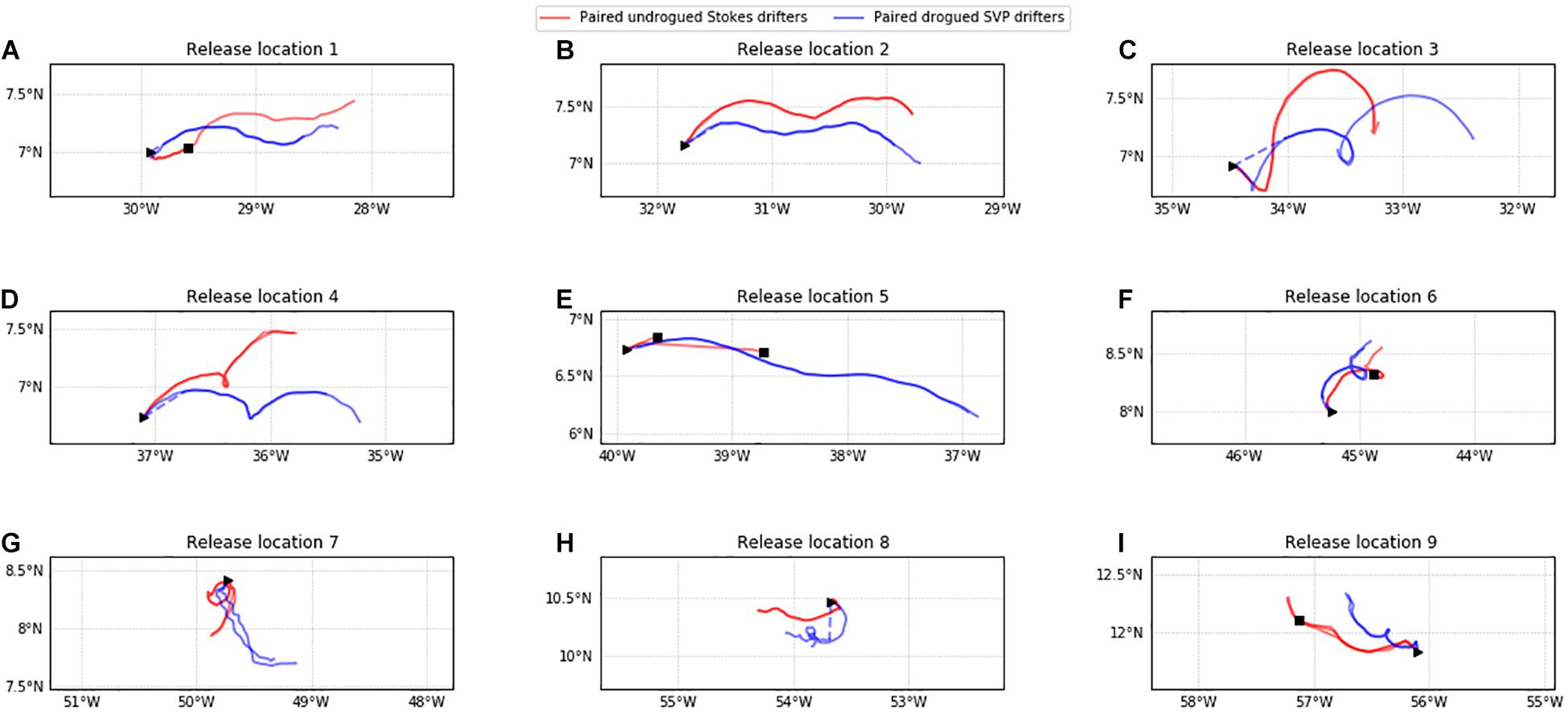
Figure 5. Maps of the drifter trajectories in the first 5 days after deployment for the nine release locations from easternmost location (A) to westernmost location (I) (black triangles), with the undrogued Stokes drifters trajectories shown in red and the drogued SVP drifters trajectories shown in blue. Note that some of the SVP drifters only started transmission a few hours to a day after deployment; the displacement between the deployment location and this first transmission is indicated by blue dashed lines. Further note that not all Stokes drifters transmitted for 5 days; locations where drifters stopped transmitting are indicated by black squares.

The separation between the different pairs (i.e., the separation between the Stokes and SVP drifters) was much larger than the within-pair separation, for all nine release locations. While the general direction of drift was similar for the Stokes and the SVP drifters, and some looping behavior was coherent between the pairs (in, e.g., release location 6), the pairs did diverge within hours of deployment.

Following the analyses in van Sebille et al. (2015), Figure 6 shows both the separation-with-time and Finites Scale Lyapunov Exponent (FSLE) analyses of the drifter dispersions. While separation-with-time, which is simply the drifter separation D (i.e., the shortest distance between the two drifters) in each pair as a function of time, is more robust to inertial oscillations (e.g., Beron-Vera and LaCasce, 2016), the FSLE analysis provided crucial information on scale-dependence of the drifter dispersion that separation-with-time cannot provide.

FIGURE 6

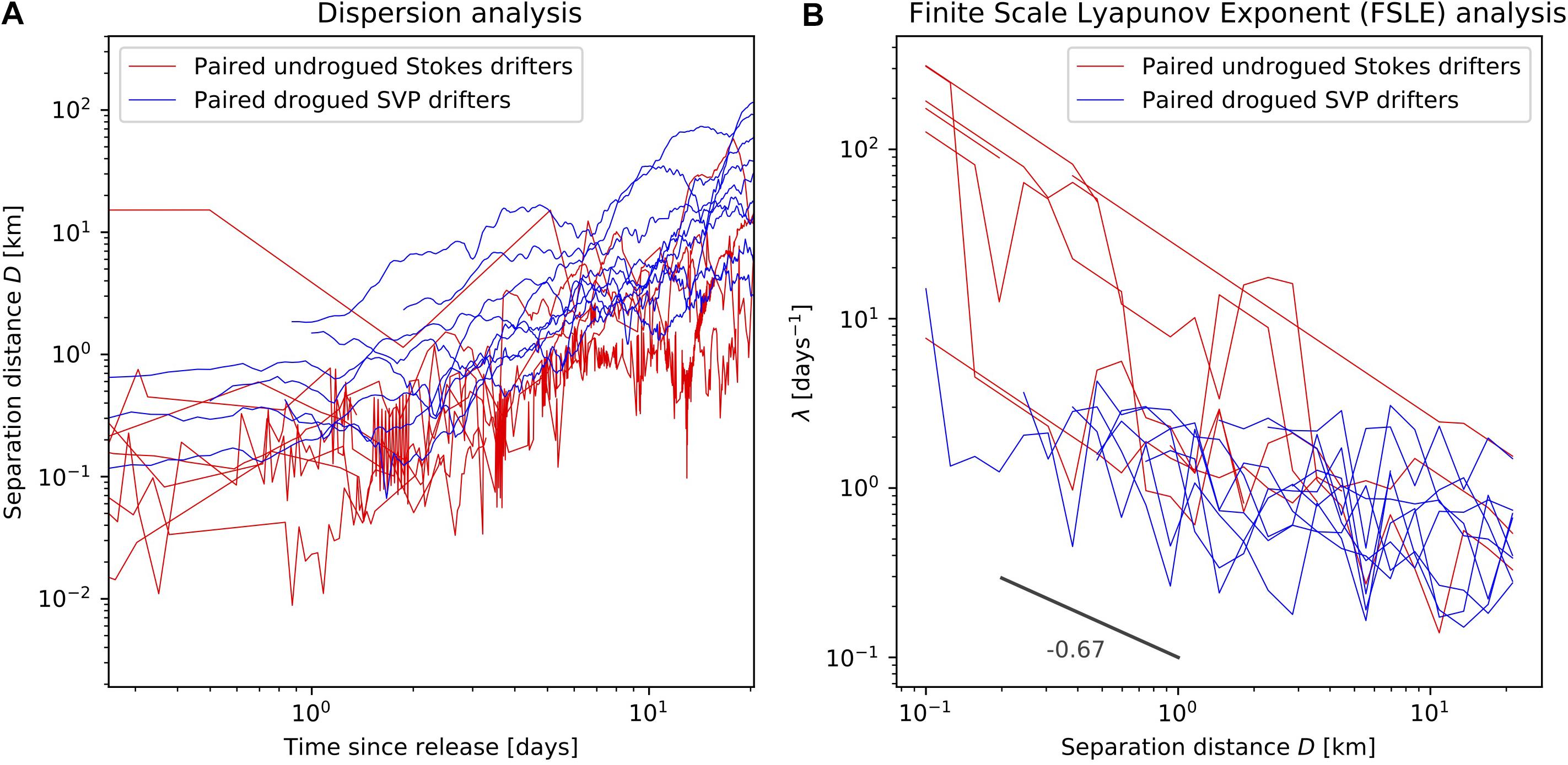
Figure 6. Pair-wise dispersion analysis for the undrogued Stokes (red) and drogued SVP (blue) drifters, shown both as separation-with-time [panel (A)] and as Finite Scale Lyapunov Exponent [FSLE, panel (B)] analyses, for the first 20 days after deployment.

In the FSLE analysis, λ(D) is the separation rate, calculated as the shortest time τ(D) on which the drifter separation D increases by a factor r, as:

$$\mathrm{\lambda }\left(D\right)=\frac{lnr}{\mathrm{\tau }(D)}$$

where we choose r = 1.25 as an optimum between reducing noise on the individual FSLE lines while maintaining resolution (see Supplementary Figure 3).

For some of the release locations (notably release locations 3, 4, and 8; see Figures 5C,D,H), the delay in start of transmission for the MétéoFrance SVP drifters meant that the first day or more of the trajectory was missed. These first hours could thus not be used for the dispersion analysis and for that reason three of the blue lines start only after one day in Figure 6A.

A very clear signal in these pairwise dispersion analyses was that the SVP drifters diverged faster than the Stokes drifters, for a given time since release. The SVP’s separation distance was on average larger than that of the Stokes drifters in Figure 6A, and for a given separation distance the separation rate was shorter in Figure 6B. This is a somewhat surprising find, which suggests that the turbulence experienced by the undrogued Stokes drifters was smaller than that experienced by the drogued SVP drifters.

One reason for the larger separation in the drogued SVP drifters could be that wind rows associated with Langmuir circulation led to stronger convergence right at the surface than at 15 m depth (e.g., Laxague et al., 2018; van Sebille et al., 2020). Indeed, Figure 6B suggests that the largest differences in FSLE separation rates between drogued and undrogued buoys occurred for scales smaller than ∼1 km, while for scales larger than ∼10 km the differences are far less striking (although data coverage for the undrogued Stokes drifters is limited beyond ∼5 km separation). This also points to dynamics on scales of hundreds seconds of meters to kilometers being the driver of these dispersion differences.

In previous work on drifter dispersion (e.g., Lumpkin and Elipot, 2010; Poje et al., 2014; van Sebille et al., 2015; Meyerjürgens et al., 2020), different scaling regimes have been identified in the FSLE analysis: A Richardson regime predicted by Surface Quasi-Geostrophic (SQG) theory where λ∝D^−2/3 (Held et al., 1995), an exponential regime predicted by Quasi-Geostrophic (QG) theory where λ is constant (e.g., Pedlosky, 1996), and a diffusive regime where λ∝D⁻² (LaCasce, 2008).

Here, we saw only the D^−2/3 Richardson regime, and possibly a shallower regime for the SVP drifters on scales between 5 and 20 km. The diffusive regime was not observed in our results, which is not a surprise as it typically only appears on length scales larger than those investigated here. That we did not find an exponential regime suggests that both the drogued SVP drifters and the undrogued Stokes drifters may follow SQG theory, and are not consistent with 2D QG turbulence, in this region. The slope in the FSLE from the undrogued Stokes drifters seemed to be slightly steeper than that in the FSLE of the drogued SVP drifters.

Comparison to Virtual Drifter Trajectories

The role of wave-driven Stokes drift on the difference in drifter transport can be further explored by comparing the observed Stokes drifter trajectories to those of virtual surface particles computed from the CMEMS-SMOC flow fields (see also section “Simulations”).

Figure 7 shows the same 5-day long trajectories as Figure 5, but now also overlays the virtual particle trajectories advected using the surface Navier-Stokes Currents, the Stokes Currents, and the Tidal Currents from CMEMS-SMOC, as well as the sum of these three components (“Total Currents”). Even though the drifter data have not been used in the SMOC data assimilation, the general pathway patterns of at least some of the virtual particles agreed well with the drifters. For some others (e.g., release locations 7 and 8), the virtual particles moved in a different direction than the drifters. Interestingly, release locations 7 and 8 were both in the Amazon plume; it could be that the edge of this plume was not captured well in SMOC.

FIGURE 7

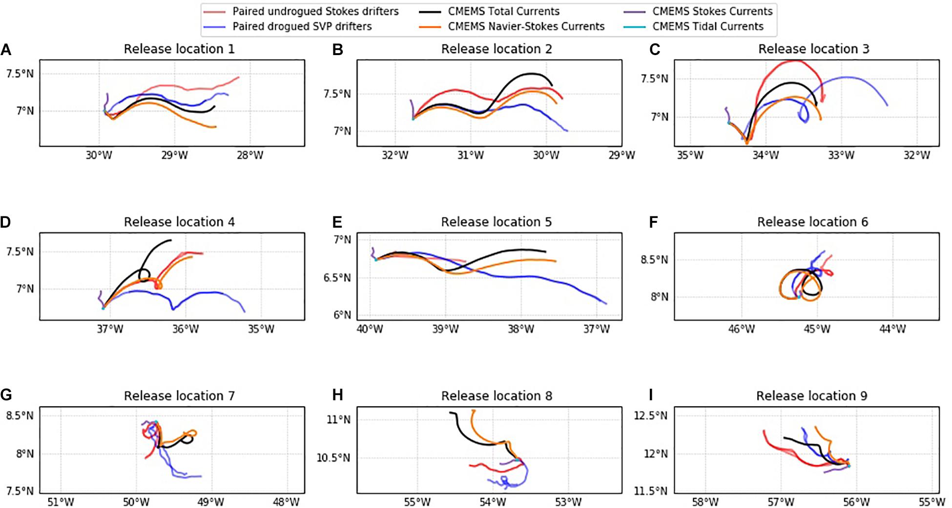
Figure 7. Comparison of observed Stokes and SVP drifters with virtual surface particles computed from the Surface and Merged Ocean Currents (SMOC) product from the Copernicus Marine Environmental Service (CMEMS). Panels (A–I) show results for easternmost location (A) to westernmost location (I).

Since we were using the surface flow fields only, our expectation was that the SMOC flow fields were in better agreement with the Stokes drifter trajectories than with the drogued SVP drifters. To quantify how the four different SMOC-based trajectories compared to the two types of drifters, we computed the mean cumulative separation distance L (Haza et al., 2019; van der Mheen et al., 2020):

$$L_i=\frac{1}{T}\sum _{t=0}^{T-1}\left|{\overrightarrow{x}}_i\left(t\right)-{\overrightarrow{x}}_{\mathit{obs}}\left(t\right)\right|$$

where ${\overrightarrow{x}}_i\left(t\right)$ is the location of virtual particle i at time t, ${\overrightarrow{x}}_{\mathit{obs}}\left(t\right)$ is the corresponding drifter location and T is the number of timesteps in the drifter trajectory. Since this metric sums over all steps in the trajectories, it provides a better measure of skill than the separation distance at the end of the trajectory alone.

The mean cumulative separation distances are shown in Figure 8. This shows, for all drifters that have transmitted at least 5 days (i.e., the ones without a black square in Figure 5), the value of L between the Stokes drifters (red S, upper rows) and SVP drifters (blue D, lower rows) and each of the four SMOC simulations, for the first 5 days and for each of the nine release locations.

FIGURE 8

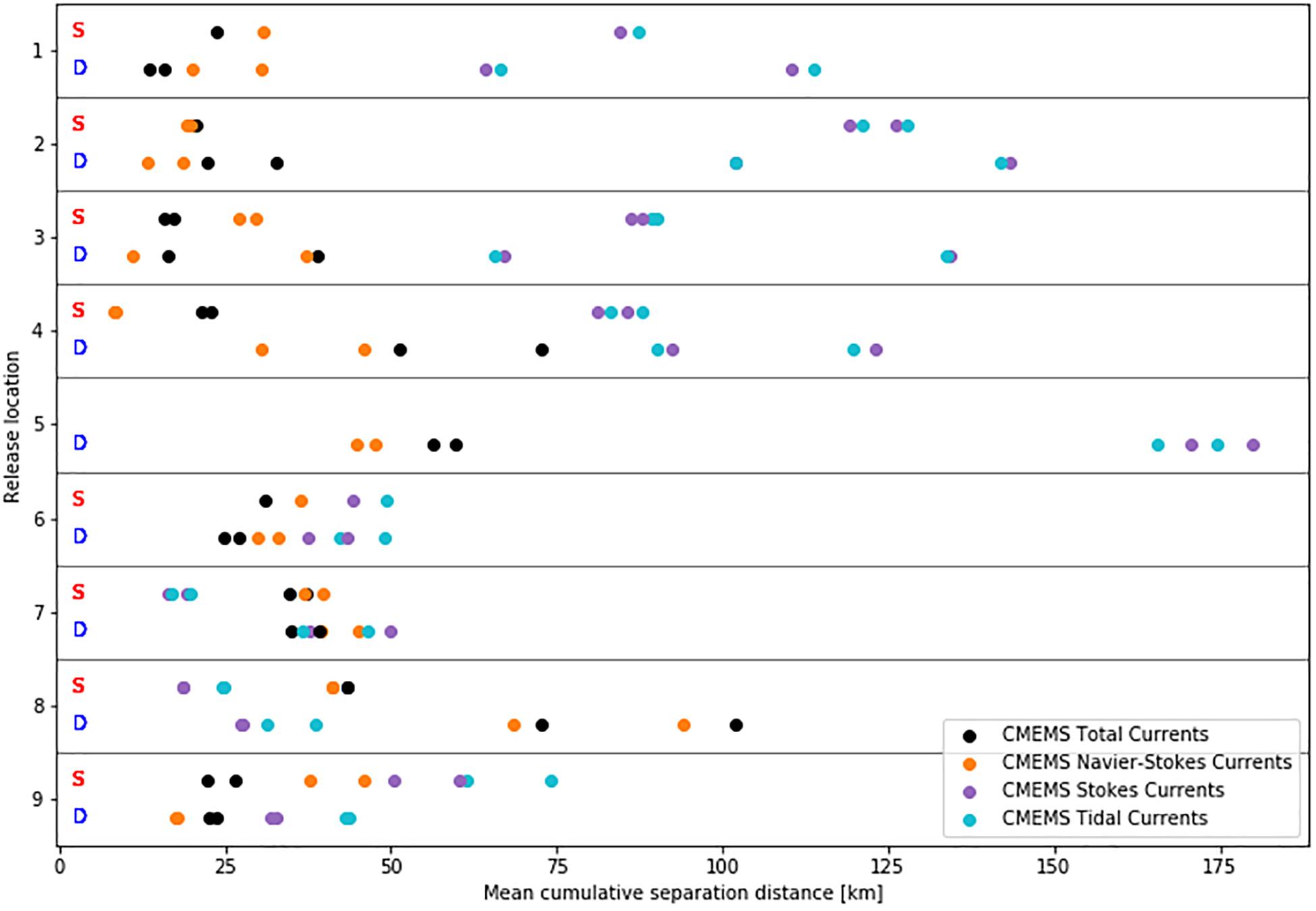
Figure 8. Mean cumulative separation distance for the first 5 days between the virtual particles advected in the CMEMS-SMOC flow fields, and the two types of drifters (undrogued Stokes drifters on the lines with red “S,” drogued SVP drifters on the lines with blue “D”), shown for each of the nine release locations. Distances were only computed for drifters that have at least 5 days of transmissions.

For most release locations, the Navier-Stokes and Total Currents yielded the smallest separation distances. For release location 7 and 8, however, the Stokes and Tidal Currents had smaller separation distances with the drifters than the Total and Navier-Stokes Currents, as could also already be seen in Figure 7. This may have to do with errors in the SMOC Navier-Stokes fields, perhaps because the release locations were on the edge of the Amazon plume, although a full investigation is beyond the scope of this work.

Unexpectedly, there was no clear pattern between the separation distances for the Stokes and SVP drifters. For three of the release locations, the smallest separation distance was with the Stokes drifters, and for five of the release locations, the smallest separation distance was with the SVP drifters (the Stokes drifters in release location 5 transmitted for less than 5 days). From this analysis alone, we could therefore not conclude that the SMOC surface currents were more representative of the Stokes drifters than of the SVP drifters, as one would expect.

Discussion and Conclusion

Here, we have presented a first analysis of the pathways and dispersion of 20 custom-built Stokes drifters and 18 regular SVP drifters in the Tropical Atlantic. This was not nearly a large enough amount to draw firm conclusions about the pathways of Sargassum into the Caribbean Sea, but it did provide insights into the difference between surface and subsurface separation. We found that the drogued SVPs separated faster than the undrogued Stokes drifters. From analyzing the full GDP data set we found that SVP drifters that had lost their drogue were more likely to enter the Caribbean Sea. We also found that the dispersion was bigger between instruments of different types (e.g., between SVP-Stokes by comparison to Stokes-Stokes and SVP-SVP), meaning that they are sensitive to different forcings.

The increase in Sargassum biomass as seen by satellites (Wang et al., 2019) has resulted in widespread strandings of sargassum mats and severe economic and environmental impacts in the Caribbean, and July 2019 satellite images estimated the largest accumulation of this macroalgae ever measured. Our drifters were deployed within that record “Great Sargassum Belt.” Despite the small dataset, because most Sargassum floats in the upper meter of the water column, our hypothesis is that the movement of Stokes drifters better represents the drift of Sargassum.

The new SMOC surface current data set from CMEMS did not capture the general pathway of the Stokes drifters that well, even though we acknowledge that individual-trajectory comparisons provide a very demanding test for models because the drifter trajectories are so sensitive to initial conditions. While for some of the release locations, the virtual and observed pathways matched nicely, for others they did not. Furthermore, the Total Currents product was not even consistently the one with the lowest mean cumulative separation distance. In some cases, the Total Currents at the surface were more similar to the drogued SVP drifters than to the undrogued Stokes drifters. This means that there is a clear need for further improvements of the surface currents product in the Tropical Atlantic Ocean, a region that plays an important role in global climate and the life cycle and fate of Sargassum.

Data Availability Statement

All codes used in this analysis are available under an MIT license at https://github.com/OceanParcels/Sargassum_Drifters. The data of the Stokes drifters is available at http://doi.org/10.5281/zenodo.4298716. The SVP data are available at ftp.aoml.noaa.gov/phod/pub/lumpkin/hourly/v1.04. The CMEMS SMOC fields are available through the motu client at http://nrt.cmems-du.eu/motu-web/Motu, using service-id GLOBAL_ANALYSIS_FORECAST_PHY_001_024-TDS and product-id global-analysis-forecast-phy-001-024-hourly-merged-uv.

Author Contributions

ES performed all analysis except for those in Figure 3 and wrote the first version of the manuscript. RL performed the analysis in Figure 3. LA-Z and EZ deployed the drifters. EZ and NW designed and constructed the Stokes drifters. All co-authors edited and revised the manuscript.

Funding

ES was partly supported through the IMMERSE project from the European Union Horizon 2020 Research and Innovation Program (grant agreement no. 821926) and the ESA World Ocean Circulation project, ESA Contract No. 4000130730/20/I-NB. RL was supported by NOAA’s Global Ocean Monitoring and Observing Program and the Atlantic Oceanographic and Meteorological Laboratory.

Conflict of Interest

The authors declare that the research was conducted in the absence of any commercial or financial relationships that could be construed as a potential conflict of interest.

Acknowledgments

The NIOZ machine and electronics shops assisted with design and construction advice for the Stokes drifters, and Philippe Delandmeter, Daan Reijnders, and Michiel Klaassen helped with final assembly. Thanks to GlobalStar for advice, and to the crew and scientists aboard NIOZ RV Pelagia cruise 64PE455.

Supplementary Material

The Supplementary Material for this article can be found online at: https://www.frontiersin.org/articles/10.3389/fmars.2020.607426/full#supplementary-material

References

Amaral-Zettler, L. A., Dragone, N. B., Schell, J., Slikas, B., Murphy, L. G., Morrall, C. E., et al. (2017). Comparative mitochondrial and chloroplast genomics of a genetically distinct form of Sargassum contributing to recent “Golden Tides” in the Western Atlantic. Ecol. Evol. 7, 516–525. doi: 10.1002/ece3.2630

PubMed Abstract | CrossRef Full Text | Google Scholar

Ardhuin, F., Aksenov, Y., Benetazzo, A., Bertino, L., Brandt, P., Caubet, E., et al. (2018). Measuring currents, ice drift, and waves from space: the Sea surface KInematics Multiscale monitoring (SKIM) concept. Ocean Sci. 14, 337–354. doi: 10.5194/os-14-337-2018

CrossRef Full Text | Google Scholar

Ardhuin, F., Brandt, P., Gaultier, L., Donlon, C., Battaglia, A., Boy, F., et al. (2019). SKIM, a candidate satellite mission exploring global ocean currents and waves. Front. Mar. Sci. 6:209. doi: 10.3389/fmars.2019.00209

CrossRef Full Text | Google Scholar

Ardhuin, F., Rogers, E., Babanin, A. V., Filipot, J.-F., Magne, R., Roland, A., et al. (2010). Semiempirical dissipation source functions for ocean waves. part i: definition, calibration, and validation. J. Phys. Oceanogr. 40, 1917–1941. doi: 10.1175/2010JPO4324.1

CrossRef Full Text | Google Scholar

Beron-Vera, F. J., and LaCasce, J. H. (2016). Statistics of simulated and observed pair separations in the gulf of mexico. J. Phys. Oceanogr. 46, 2183–2199. doi: 10.1175/JPO-D-15-0127.1

CrossRef Full Text | Google Scholar

Carrere, L., Lyard, F., Cancet, M., and Guillot, A. (2015). FES 2014, A New Tidal Model on the Global Ocean with Enhanced Accuracy in Shallow Seas and in the Arctic Region. Austria: EGU General Assembly.

Google Scholar

Coston-Clements, L., Settle, L. R., Hoss, D. E., and Cross, F. A. (1991). Utilization of the Sargassum Habitat by Marine Invertebrates and Vertebrates, A Review. Memo: NOAA Tech.

Google Scholar

Delandmeter, P., and van Sebille, E. (2019). The parcels v2.0 lagrangian framework: new field interpolation schemes. Geosci. Model Dev. 12, 3571–3584. doi: 10.5194/gmd-12-3571-2019

CrossRef Full Text | Google Scholar

Elipot, S., Lumpkin, R., Perez, R. C., Lilly, J. M., Early, J. J., and Sykulski, A. M. (2016). A global surface drifter data set at hourly resolution. J. Geophys. Res. 121, 2937–2966. doi: 10.1002/2016JC011716

CrossRef Full Text | Google Scholar

Fraser, C. I., Morrison, A. K., Hogg, A. M., Macaya, E. C., van Sebille, E., Ryan, P. G., et al. (2018). Antarctica’s ecological isolation will be broken by storm-driven dispersal and warming. Nat. Clim. Change 8, 704–708. doi: 10.1038/s41558-018-0209-7

CrossRef Full Text | Google Scholar

Gasparin, F., Greiner, E., Lellouche, J.-M., Legalloudec, O., Garric, G., Drillet, Y., et al. (2018). A large-scale view of oceanic variability from 2007 to 2015 in the global high resolution monitoring and forecasting system at Mercator Océan. J. Mar. Syst. 187, 260–276. doi: 10.1016/j.jmarsys.2018.06.015

CrossRef Full Text | Google Scholar

Gower, J., and King, S. (2019). Seaweed, seaweed everywhere. Science 365, 27–27. doi: 10.1126/science.aay0989

PubMed Abstract | CrossRef Full Text | Google Scholar

Haza, A. C., Paldor, N., Özgökmen, T. M., Curcic, M., Chen, S. S., and Jacobs, G. (2019). Wind-based estimations of ocean surface currents from massive clusters of drifters in the gulf of mexico. J. Geophys. Res. 124, 5844–5869. doi: 10.1029/2018JC014813

CrossRef Full Text | Google Scholar

Haza, A. C., Poje, A. C., Ozgokmen, T. M., and Martin, P. J. (2008). Relative dispersion from a high-resolution coastal model of the Adriatic Sea. Ocean Model. 22, 48–65. doi: 10.1016/j.ocemod.2008.01.006

CrossRef Full Text | Google Scholar

Held, I. M., Pierrehumbert, R. T., Garner, S. T., and Swanson, K. L. (1995). Surface quasi-geostrophic dynamics. J. Fluid Mech. 282, 1–20. doi: 10.1017/S0022112095000012

CrossRef Full Text | Google Scholar

Hummels, R., Dengler, M., Brandt, P., and Schlundt, M. (2014). Diapycnal heat flux and mixed layer heat budget within the Atlantic Cold Tongue. Clim. Dyn. 43, 3179–3199. doi: 10.1007/s00382-014-2339-6

CrossRef Full Text | Google Scholar

Johns, E. M., Lumpkin, R., Putman, N. F., Smith, R. H., Muller-Karger, F. E., Rueda-Roa, D. T., et al. (2020). The establishment of a pelagic Sargassum population in the tropical Atlantic: biological consequences of a basin-scale long distance dispersal event. Progr. Oceanogr. 182:102269. doi: 10.1016/j.pocean.2020.102437

CrossRef Full Text | Google Scholar

Johnson, D. L., and Richardson, P. L. (1977). On the wind-induced sinking of Sargassum. J. Exp. Mar. Biol. Ecol. 28, 255–267. doi: 10.1016/0022-0981(77)90095-8

CrossRef Full Text | Google Scholar

Jutzeler, M., Marsh, R., van Sebille, E., Mittal, T., Carey, R. J., Fauria, K. E., et al. (2020). Ongoing dispersal of the 7 august 2019 pumice raft from the tonga arc in the southwestern pacific ocean. Geophys. Res. Lett. 47:e1701121. doi: 10.1029/2019GL086768

CrossRef Full Text | Google Scholar

LaCasce, J. H. (2008). Statistics from Lagrangian observations. Prog. Oceanogr. 77, 1–29. doi: 10.1016/j.pocean.2008.02.002

CrossRef Full Text | Google Scholar

Laxague, N. J. M., Özgökmen, T. M., Haus, B. K., Novelli, G., Shcherbina, A., Sutherland, P., et al. (2018). Observations of near-surface current shear help describe oceanic oil and plastic transport. Geophys. Res. Lett. 45, 245–249. doi: 10.1002/2017GL075891

CrossRef Full Text | Google Scholar

Lumpkin, R., and Centurioni, L. (2019). NOAA Global Drifter Program Quality-Controlled 6-Hour Interpolated Data from Ocean Surface Drifting Buoys. Washington, DC: NOAA.

Google Scholar

Lumpkin, R., and Elipot, S. (2010). Surface drifter pair spreading in the North Atlantic. J. Geophys. Res. 115:C12017. doi: 10.1029/2010JC006338

CrossRef Full Text | Google Scholar

Lumpkin, R., and Garzoli, S. L. (2005). Near-surface circulation in the Tropical Atlantic Ocean. Deep Sea Res. I Oceanogr. Res. Pap. 52, 495–518. doi: 10.1016/j.dsr.2004.09.001

CrossRef Full Text | Google Scholar

Lumpkin, R., Ozgokmen, T. M., and Centurioni, L. (2017). Advances in the application of surface drifters. Annu. Rev. Mar. Sci. 9, 59–81. doi: 10.1146/annurev-marine-010816-060641

PubMed Abstract | CrossRef Full Text | Google Scholar

Lumpkin, R., and Pazos, M. (2007). “Measuring surface currents with surface velocity program drifters: the instrument, its data, and some recent results,” in Lagrangian Analysis and Prediction of Coastal and Ocean Dynamics, eds A. D. Jr Kirwan, A. Griffa, A. J. Mariano, H. T. Rossby, and T. Özgökmen (Cambridge: Cambridge University Press), 39–67. doi: 10.1017/CBO9780511535901.003

CrossRef Full Text | Google Scholar

Madec, G., and NEMO Team (2016). NEMO Ocean Engine. Guyancour: Institut Pierre-Simon Laplace (IPSL).

Google Scholar

Meyerjürgens, J., Ricker, M., Schakau, V., Badewien, T. H., and Stanev, E. V. (2020). Relative Dispersion of surface drifters in the north sea: the effect of tides on mesoscale diffusivity. J. Geophys.Res. 125:e2019JC015925. doi: 10.1029/2019JC015925

CrossRef Full Text | Google Scholar

Michotey, V., Blanfuné, A., Chevalier, C., Garel, M., Diaz, F., Berline, L., et al. (2020). In situ observations and modelling revealed environmental factors favouring occurrence of Vibrio in microbiome of the pelagic Sargassum responsible for strandings. Science of The Total Environment 748:141216. doi: 10.1016/j.scitotenv.2020.141216

PubMed Abstract | CrossRef Full Text | Google Scholar

Morey, S. L., Wienders, N., Dukhovskoy, D. S., and Bourassa, M. A. (2018). Measurement characteristics of near-surface currents from ultra-thin drifters, drogued drifters, and HF radar. Remote Sens. 10:1633. doi: 10.3390/rs10101633

CrossRef Full Text | Google Scholar

Onink, V., Wichmann, D., Delandmeter, P., and van Sebille, E. (2019). The role of Ekman currents, geostrophy and Stokes drift in the accumulation of floating microplastic. J. Geophys. Res. 124, 1474–1490. doi: 10.1029/2018JC014547

PubMed Abstract | CrossRef Full Text | Google Scholar

Pedlosky, J. (1996). Ocean Circulation Theory. Berlin: Springer-Verlag.

Google Scholar

Poje, A. C., Ozgokmen, T. M., Lipphardt, B. L., Haus, B. K., Ryan, E. H., Haza, A. C., et al. (2014). Submesoscale dispersion in the vicinity of the Deepwater Horizon spill. Proc. Natl. Acad. Sci. U.S.A. 111, 12693–12698. doi: 10.1073/pnas.1402452111

PubMed Abstract | CrossRef Full Text | Google Scholar

Putman, N. F., Goni, G. J., Gramer, L. J., Hu, C., Johns, E. M., Trinanes, J., et al. (2018). Simulating transport pathways of pelagic Sargassum from the Equatorial Atlantic into the Caribbean Sea. Prog. Oceanogr. 165, 205–214. doi: 10.1016/j.pocean.2018.06.009

CrossRef Full Text | Google Scholar

Putman, N. F., Lumpkin, R., Olascoaga, M. J., Trinanes, J., and Goni, G. J. (2020). Improving transport predictions of pelagic Sargassum. J. Exper. Mar. Biol. Ecol. 529:151398. doi: 10.1016/j.jembe.2020.151398

CrossRef Full Text | Google Scholar

Schell, J. M., Goodwin, D. S., and Siuda, A. N. S. (2015). Recent sargassum inundation events in the caribbean: shipboard observations reveal dominance of a previously rare form. Oceanography 28, 8–11. doi: 10.5670/oceanog.2015.70

CrossRef Full Text | Google Scholar

Schlundt, M., Brandt, P., Dengler, M., Hummels, R., Fischer, T., Bumke, K., et al. (2014). Mixed layer heat and salinity budgets during the onset of the 2011 Atlantic cold tongue. J. Geophys. Res. 119, 7882–7910. doi: 10.1002/2014JC010021

CrossRef Full Text | Google Scholar

Sutherland, G., Soontiens, N., Davidson, F., Smith, G. C., Bernier, N., Blanken, H., et al. (2020). Evaluating the leeway coefficient of ocean drifters using operational marine environmental prediction systems. J. Atmos. Ocean. Technol. 37, 1943–1954. doi: 10.1175/JTECH-D-20-0013.1

CrossRef Full Text | Google Scholar

van den Bremer, T. S., and Breivik, Ø (2018). Stokes drift. Phil. Trans. R. Soc. A Math. Phys. Eng. Sci. 376:20170104. doi: 10.1098/rsta.2017.0104

PubMed Abstract | CrossRef Full Text | Google Scholar

van der Mheen, M., Pattiaratchi, C., Cosoli, S., and Wandres, M. (2020). Depth-dependent correction for wind-driven drift current in particle tracking applications. Front Mar Sci 7:305. doi: 10.3389/fmars.2020.00305

CrossRef Full Text | Google Scholar

van Sebille, E., Aliani, S., Law, K. L., Maximenko, N., Alsina, J. M., Bagaev, A., et al. (2020). The physical oceanography of the transport of floating marine debris. Environ. Res. Lett. 15:023003. doi: 10.1088/1748-9326/ab6d7d

CrossRef Full Text | Google Scholar

van Sebille, E., Beal, L. M., and Johns, W. E. (2011). Advective time scales of Agulhas leakage to the North Atlantic in surface drifter observations and the 3D OFES model. J. Phys. Oceanogr. 41, 1026–1034. doi: 10.1175/2010JPO4602.1

CrossRef Full Text | Google Scholar

van Sebille, E., Waterman, S., Barthel, A., Lumpkin, R., Keating, S. R., Fogwill, C., et al. (2015). Pairwise surface drifter separation in the western Pacific sector of the Southern Ocean. J. Geophys. Res. 120, 6769–6781. doi: 10.1002/2015JC010972

CrossRef Full Text | Google Scholar

Wang, M., Hu, C., Barnes, B. B., Mitchum, G., Lapointe, B., and Montoya, J. P. (2019). The great Atlantic Sargassum belt. Science 365, 83–87. doi: 10.1126/science.aaw7912

PubMed Abstract | CrossRef Full Text | Google Scholar

Wichmann, D., Delandmeter, P., and van Sebille, E. (2019). Influence of near-surface currents on the global dispersal of marine microplastic. J. Geophys. Res. 124, 6086–6096. doi: 10.1029/2019JC015328

CrossRef Full Text | Google Scholar