Physical and Biogeochemical Regionalization of the Southern Ocean and the CCAMLR Zone 48.1

Introduction

The Southern Ocean plays a major role in the Earth’s climate since the opening of the Drake Passage approximately 41 Ma ago (Scher and Martin, 2006). The Antarctic Circumpolar Current is the major current of the planet (with a transport of 137 Sv; Rintoul and da Silva, 2019) and it connects the Pacific, Indian and Atlantic Ocean basins isolating the Antarctic continent from lower latitudes. The Antarctic Circumpolar Current and the Southern Ocean influence heat and salt balances and biogeochemical cycles (e.g., C, N, P; Sallée, 2018). The combination of the thermohaline gradient, sea-ice cycle and atmospheric patterns creates a meridional overturning circulation in the Southern Ocean (Tomczak and Godfrey, 2003; Morrison et al., 2015) which is a sensitive mechanism able to influence the greenhouse gases budget between the atmosphere and the ocean (Reid et al., 2009; Gruber et al., 2019). The export of Particulate Organic Carbon (POC) south of 50°S is 1000 Tg C yr^–1 corresponding to 10% of the global POC export, with a significant contribution of dissolved organic carbon in the top 500 m of the water column (Schlitzer, 2002). The Southern Ocean has also been identified as a region providing important ecosystem services, particularly fisheries (CCAMLR, 2018; FAO, 2018) and maintenance of biodiversity (Grant et al., 2013; David and Saucède, 2015).

The Southern Ocean is recognized as a High Nutrient Low Chlorophyll region, approximately 48% of the Southern Ocean mean surface Chlorophyll-a (Chl-a) concentration is lower than 0.25 mg m^–3 despite high macronutrients concentration (Pollard et al., 2006). Different hypotheses have been proposed, from light limitation due to deep mixing (Venables and Moore, 2010) to zooplankton grazing pressure (Le Quéré et al., 2016) and bioavailable dissolved iron depletion (Martin et al., 1990; Wadley et al., 2014). The iron limitation hypothesis leaded to several expeditions between 1993 and 2011 to artificially fertilize the photic layer of the Southern Ocean, these experiments increased surface Chl-a up to 15-fold (Boyd et al., 2007; Yoon et al., 2018). Pitchford and Brindley (1999) suggested that different explanations should be regarded as complementary, rather than alternative. The oceanic islands of the Southern Ocean (e.g., South Georgia Islands) stand out from High Nutrient Low Chlorophyll productivity patterns, mainly due to local input of dissolved iron and shallower bathymetry (Venables and Moore, 2010).

The 48.1 zone of the Commission for the Conservation of Antarctic Marine Living Resources (CCAMLR) is a key region for monitoring the Antarctic ecosystem. This area is experimenting strong interannual variability and trends in sea ice coverage and water column temperature (Schmidtko et al., 2014; Jones et al., 2016) that turn this zone in one of the most climate sensitive region of the planet and most variable (Hendry et al., 2018). Recent studies (Murphy et al., 2016; Comiso et al., 2017) suggested that the interannual oceanographic variability is partly linked with atmospheric patterns, such as El Niño-Southern Oscillation and the Southern Annular Mode. This region is subject to strong anthropic influence via krill fisheries (Boyd, 2009; Ainley and Pauly, 2014; McBride et al., 2014) and local contamination by increasing tourist’s presence (Bargagli, 2008; Waller et al., 2017). Intense Antarctic krill (Euphausia superba) fisheries within the 48.1 zone (Brooks et al., 2018) might have important repercussion on the trophic structure and the trophic pathways due to the reduced functional redundancy of polar ecosystems (i.e., few species perform most of the ecological functions; Murphy et al., 2016), the key role of krill within the Antarctic food web (Trivelpiece et al., 2011; Murphy et al., 2012; McBride et al., 2014) and the importance of this region for krill spawning and nursery (Piñones and Fedorov, 2016; Henley et al., 2019; Perry et al., 2019). A specific focus was given to CCAMLR 48.1 zone because of the ecological importance of this climate sensitive area and since no other biogeochemical regionalization study has been previously developed for this region according to our knowledge.

Regionalization is an important tool for conservation and management of the marine environment and marine resources, since it can provide useful information for identification of protected areas and fisheries zones (Berline et al., 2014). Marine protected areas are multi-purpose regions that provide protection for the natural resources they contain and can help marine ecosystems be resilient to natural and anthropic-driven climate changes (Roberts et al., 2017). Currently, the Ross Sea and the South Orkney Islands are the only established marine protected areas within the Southern Ocean, while three more proposal have been submitted for East Antarctica, the Antarctic Peninsula and the Weddell Sea (Sylvester and Brooks, 2020). The terrestrial ice-free area of Antarctica was divided in 16 biogeographic regions by Terauds and Lee (2016), whereas various studies of bioregionalization have been previously performed for the Southern Ocean pelagic (i.e., Grant et al., 2006; Spalding et al., 2007, 2012; Cabré et al., 2016) and benthic communities (Griffiths et al., 2009; Pierrat et al., 2013; Douglass et al., 2014; Hogg et al., 2016; Teschke et al., 2016; Fabri-Ruiz et al., 2020). A new physical and biogeochemical regionalization is needed to fill the existing gap in the understanding of the physical forcing on biogeochemical cycles spatial heterogeneity (Hendry et al., 2018) and to generate useful information for marine protected areas proposals and marine ecosystem modeling.

This study will generate new physical and biogeochemical regionalization utilizing the Southern Ocean data available from satellite-derived and model output databases. The degree of similarity between physical and biogeochemical characteristics obtained with this new regionalization will be compared with previously existing regionalization. In addition, the physical variable that primarily control biogeochemical variability in the Southern Ocean and CCAMLR 48.1 zone will be identified. The work will deliver useful information to the scientific community in order to identify highly productive areas and to understand and predict future changes in the context of the current climate crisis.

Materials and Methods

Study Zone

The International Hydrographic Organization (IHO, 2002) defined the northerner limits of the Southern Ocean at 60°S. For the purpose of this study, the northern limit of the Southern Ocean was set at 50°S due to the spatial distribution of the Polar and Subantarctic Fronts (Orsi et al., 1995; Sallée et al., 2008; Koshlyakov and Tarakanov, 2011), especially in the Atlantic and western Indian Ocean (Figure 1). The proposed limit allowed the inclusion of the entire Drake Passage and the Southern Patagonia, permitting the analysis of differences and similarities between Antarctic and Subantarctic habitats from a physical and a biogeochemical oceanographic point of view.

FIGURE 1

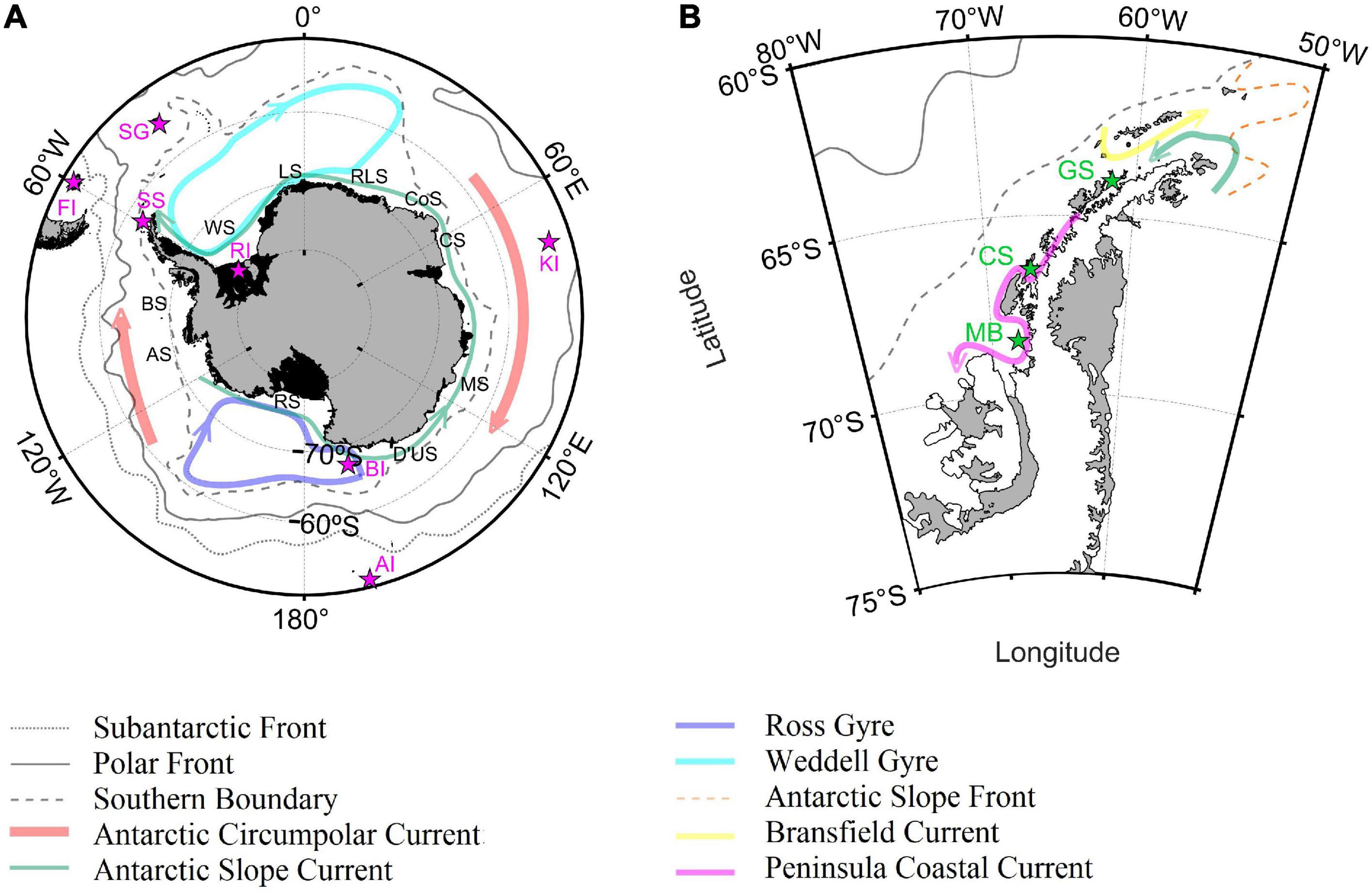
Figure 1. Geographic location of the main islands, places, fronts, seas and circulation patterns for the Southern Ocean (A) and CCAMLR 48.1 zone (B). Magenta and green stars indicated the location of Falkland Islands (FI); SG,South Georgia Island; SS, South Shetland Islands; RI, Ronne ice shelf; BI, Balleny Islands; AI, Auckland Islands; KI, Kerguelen Islands; MB, Marguerite Bay; CS, Crystal Sound; GS, Gerlache Strait. Black letters indicated the location of the main Antarctic seas: Bellingshausen Sea (BS); AS, Amundsen Sea; RS, Ross Sea; D’US, D’Urville Sea; MS, Mawson Sea; CS, Cooperation Sea; CoS, Cosmonaut Sea; RLS, Riiser-Larsen Sea; LS, Lazarev Sea; WS, Weddell Sea. Fronts location was obtained from Orsi et al. (1995), whereas the circulation patterns were reproduced combining the information from Heywood et al. (2004); Thompson et al. (2009), Armitage et al. (2018); Moffat and Meredith (2018), Thompson et al. (2018), and Vernet et al. (2019).

The limits of the CCAMLR 48.1 zone (50–70°W, 60–70°S with the exclusion of the of the southern part of the Weddell Sea) are in fact very similar to those that define the Western Antarctic Peninsula and Scotia Arc zone identified by the Southern Ocean Observing System¹. The 48.1 zone include the shelves and pelagic areas off the Western Antarctic Peninsula from Margarite Bay to the tip of the Peninsula (Figure 1), coastal islands such as the South Shetland Islands and the northern part of the Eastern Antarctic Peninsula. This study dedicated a special focus on the CCAMLR 48.1 zone because it is one of the most important spawning regions for Antarctic krill (Perry et al., 2019) that is directly affected by fisheries (Ainley and Pauly, 2014; Brooks et al., 2018) and has experienced one of the fastest temperature increase of the planet (Turner et al., 2005, 2016). Krill was the main fishery target within the 48.1 zone and represented the 99.9% of the catches in the area since 2000 (CCAMLR, 2018). Krill landings from the 48.1 zone accounted for 45% of total Southern Ocean krill catches and the eastern and western part of the Bransfield Strait were the regions where most of the 48.1 krill catches occurred (62%), followed by the western pelagic area of the Drake Passage (15%). Most of these catches were made with midwater otter trawls (CCAMLR, 2018).

Physical and Biogeochemical Variables

The variables selected for the physical and biogeochemical regionalization, along with their characteristics, are presented in Table 1. The mean value of the physical and biogeochemical parameters during the “productivity season” (December–March; Supplementary Figures 1, 2) was calculated in a 1° × 1° latitude/longitude grid south of 50°S. The study focused on this period based on the phenology of phytoplankton proliferations (Soppa et al., 2016), the higher krill abundances (Atkinson et al., 2017) and the higher proportion of valid satellite data with respect to austral winter. The majority of the analyzed variables covered a time span of 15 years (2003–2018), with the significant exception of iron concentration and mixed layer depth (MLD) estimations that only were available for a period of 5 years (Table 1). These model-output databases were chosen despite of their limited time frame because they guaranteed a higher spatial coverage with respect to others in situ databases (i.e., Tagliabue et al., 2012; Li et al., 2017; Holte et al., 2017), especially in the coastal areas of the Antarctic continent.

TABLE 1

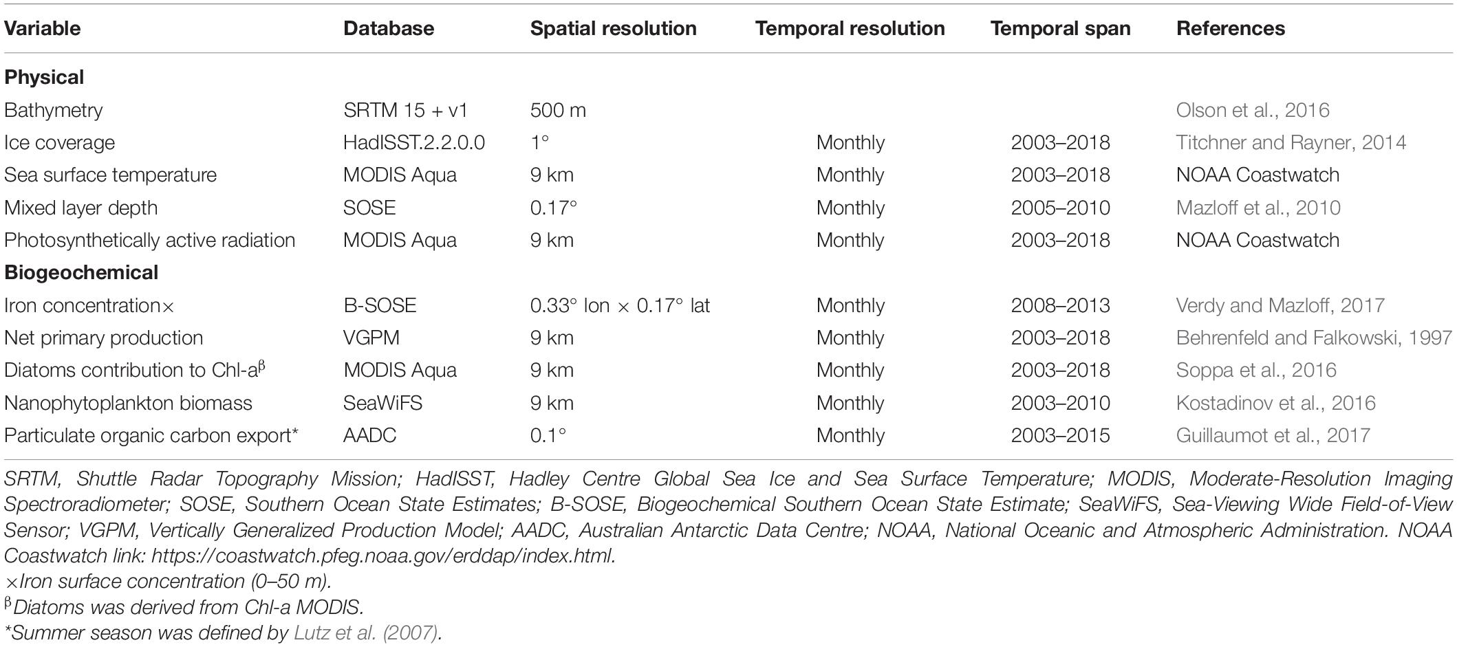
Table 1. Spatio-temporal characteristics of the physical and biogeochemical variables used in this study.

Olson et al. (2016) bathymetry data was obtained from the data.gov portal², whereas Titchner and Rayner (2014) sea ice estimations were downloaded from the Met Office Hadley Center page³. Monthly composite of satellite-derived variables (sea surface temperature, photosynthetically active radiation and chlorophyll-a; SST, PAR and Chl-a, respectively) were extracted from the CoastWatch project of the National Oceanic and Atmosphere Administration⁴. Model output variables, such as MLD and iron concentration in the surface water, were obtained from the Southern Ocean State Estimation page⁵. Net Primary Production (NPP) estimations calculated with the “standard” Vertically Generalized Production Model (Behrenfeld and Falkowski, 1997) were acquired from the Ocean Productivity page⁶. Finally, Kostadinov et al. (2016) nanophytoplankton concentration was achieved from the PANGEA data center⁷ and Particulate Organic Carbon (POC) exports were extracted from the Australian Antarctic Data Center⁸.

It is important to consider that satellite-derived Chl-a was directly used as input parameter for NPP, diatoms and POC export estimations, which may cause redundancy in the spatial variability of these variables and the biogeochemical regionalization. In spite of this, the treatment of Chl-a data was different for each product, since only diatoms concentration exclusively relies on Chl-a concentration and NPP and POC estimations used multiple input variables along with Chl-a data. Soppa et al. (2016) equation was used for diatoms concentration: log₁₀(Diatom) = 1.1559⋅log₁₀(Chl-a) − 0.2901. Behrenfeld and Falkowski (1997) equation for NPP estimations might be summarized as: NPP = f(Chl-a) ^⋅ f(SST) ^⋅ D_L ^⋅ f(PAR); where f(Chl-a) represents a function of surface Chlorophyll-a estimation, f(SST) indicates a function of Sea Surface Temperature, D_L is the day length and f(PAR) represents a function of Photosynthetically Active Radiation. On the other hand, POC export flux was calculated by Guillaumot et al. (2017) using: POC export = NPP_c ^⋅ f(Z_eu) ^⋅ f(Z₀); where NPP_c is the Net Primary Production in the surface water calculated with the Carbon-based Production Model (Westberry et al., 2008), Z_eu indicates the depth of the euphotic zone and Z₀ the depth of the sea floor. The simplified equation for NPP_c might be summarize as: NPP_c = f(Chl-a) ^⋅ f(bbp) ^⋅ f(PAR) ^⋅ f(Z_NO3) ^⋅ D_L ^⋅ f(MLD) ^⋅ f(k₄₉₀); where f(bbp) indicates a function of the particulate backscattering coefficient at 443 nm, f(Z_NO3) is a function of nitracline depth, f(MLD) represents a function of Mixed Layer Depth and f(k₄₉₀) is a function of the diffuse attenuation coefficient at 490 nm.

Estimates of Regionalization

Regionalization is a useful methodological tool that allows to identify similarities and dissimilarities between adjacent and remote areas according to different criteria and to group regions with analogous properties. Indeed, a regionalization developed using physical variables might provide the degree of similarity (expressed as distance in a dendrogram) between regions from a physical standpoint. On the other hand, the use of biogeochemical variables will result in a regionalization according to a biogeochemical point of view. The number of regions provided by this analysis is an indicator of heterogeneity; whereas the mean value for each group (i.e., cluster) might help the identification of areas with similar temperature and sea ice patterns as well as high and low productivity zones. The comparison between physical and biogeochemical regionalization can provide useful information about physical and biogeochemical patterns within a defined area.

The Southern Ocean regionalization was developed following the methodology of Grant et al. (2006) and Raymond (2014). The main steps for this analysis were: (I) The mean bathymetry for each pixel was transformed in log₁₀(bathymetry); (II) the pixels with at least a missing value among all variables were eliminated (i.e., no interpolation was used); (III) all the variables were normalized between 0 and 1; (IV) non-hierarchical Clustering Large Application (CLARA; Kaufman and Rousseeuw, 1990) was applied to group all the pixels within 250 clusters using Manhattan distance for both datasets as indicated by Grant et al. (2006) and Raymond (2014); (V) the mean value for each of the 250 groups was calculated; (VI) an agglomerative hierarchical clustering method (Unweighted Pair Group Method with Arithmetic mean, UPGMA; Sokal and Michener, 1958) was applied to the results of the previous step; (VII) the number of significant clusters within the data was identified using the Clarke et al. (2008) statistical method (1000 permutations and an alpha value of 0.05 with the assumption of no a priori groups). This section slightly modified the original methodology proposed by Grant et al. (2006), which incorporated a cutoff method for dendrograms. Indeed, the cutoff technique strongly depends on authors criteria, whereas other “traditional” methods to determine numbers of clusters within a dendrogram (i.e., elbow, silhouette, gap statistic and Charrad et al. (2014) methods) were unsuccessful when applied to the data (Supplementary Table 1). On the contrary, the regionalization of CCAMLR 48.1 zone was performed exclusively with UPGMA agglomerative cluster due to reduced sample size. The analyses were carried out using R⁹ and Matlab¹⁰.

The regionalization methodology applied in this study is accompanied by different sources of uncertainties in the pixels grouping and boundaries location between areas. Among different factors, uncertainty might be ascribed to imprecision in the data and epistemic uncertainty related to the knowledge of regionalization process (Grant et al., 2006). Data imprecisions comprise satellite or model estimations errors and bias due to incomplete observations, whereas knowledge errors include the data selection and the processing steps, such as the clustering method.

Relationship Between Physical and Biogeochemical Variables and Regions

The Pearson linear correlation coefficient (p-value: 0.05) between physical and biogeochemical variables, along with the geographical coordinates, was estimated. The BIO-ENV package from Clarke and Ainsworth (1993) was used in order to find the best subset of physical variables that have maximum correlation with biogeochemical dissimilarities throughout Spearman rank correlation coefficient. In addition, Distance-Based Redundancy Analysis (db-RDA; Legendre and Andersson, 1999), which is the direct extension of multiple regression to the multivariate scale and it allows non-Euclidean dissimilarity indices (i.e., Manhattan distance), was performed with 1,000 permutations and a p-value of 0.001. Throughout db-RDA analysis the ordination process was constrained by the biogeochemical variables and the ordination sought the axes that were best explained by a linear combination of explanatory physical variables (Kindt and Coe, 2005; Borcard et al., 2018). An analysis of variance (ANOVA) was performed to assess the significance of constraints. Both BIO-ENV and db-RDA analysis were realized using the R package Vegan from Oksanen et al. (2019).

For every biogeochemical region the number of physical clusters in which it was divided (and vice versa) were calculated in order to evaluate the degree of agreement between physical and biogeochemical regionalization. The clusters that represented less than 20% of total pixels of the corresponding region were filtered to identify the zones that majorly contributes to its surface. Finally, a non-parametric Mann–Kendall test for significance (with a p-value < 0.05) was used to assess the statistical significance of sea ice trend.

Results

Southern Ocean

Physical Regionalization

The Southern Ocean presented very heterogenous physical conditions during the biological productive season (December to March). Sea ice coverage, indeed, ranged from 0 to 99%, whereas MLD varied between 12 and 103 m and SST (with a mean value of 2°C) oscillated between −1 and 12°C (Table 2). Physical variables were grouped in an agglomerative hierarchical cluster tree with a cophenetic correlation coefficient of 0.73 (Figure 2A) and 12 significant clusters were identified within the dendrogram (Figure 2B). Two oceanic ice-free zones north of 60°S (clusters n° 11 and 12) characterized by deep bathymetry and MLD (Supplementary Table 2) covered approximately the 53% of the study zone (38 and 15%, respectively). On the other hand, regions south of the Polar Front (clusters from n° 1 to 9) were characterized by low SST (mean values ranged from −0.96 to 0.47°C), shallow MLD (varying between 23.13 to 34.42 m) and reduced PAR values (from 14.34 to 27.87 E m^–2 d^–1). The areas of Falkland Islands and South America were merged within one cluster (n° 10) that presented few pixels with shallow bathymetry, no ice coverage and highest PAR and SST values. Clear circum-Antarctic patterns were detected in several oceanic regions north (n° 8, 11, and 12) and south (n° 2 and 3) of 60°S, whereas this circumpolar structure was absent for coastal clusters (Figure 2B).

TABLE 2

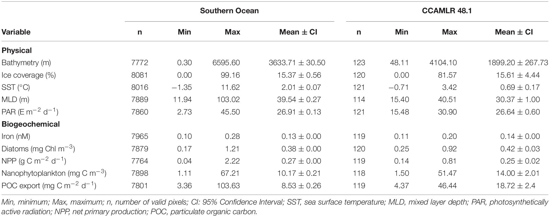
Table 2. Basic statistics of physical and biogeochemical variables within Southern Ocean and CCAMLR 48.1 zone.

FIGURE 2

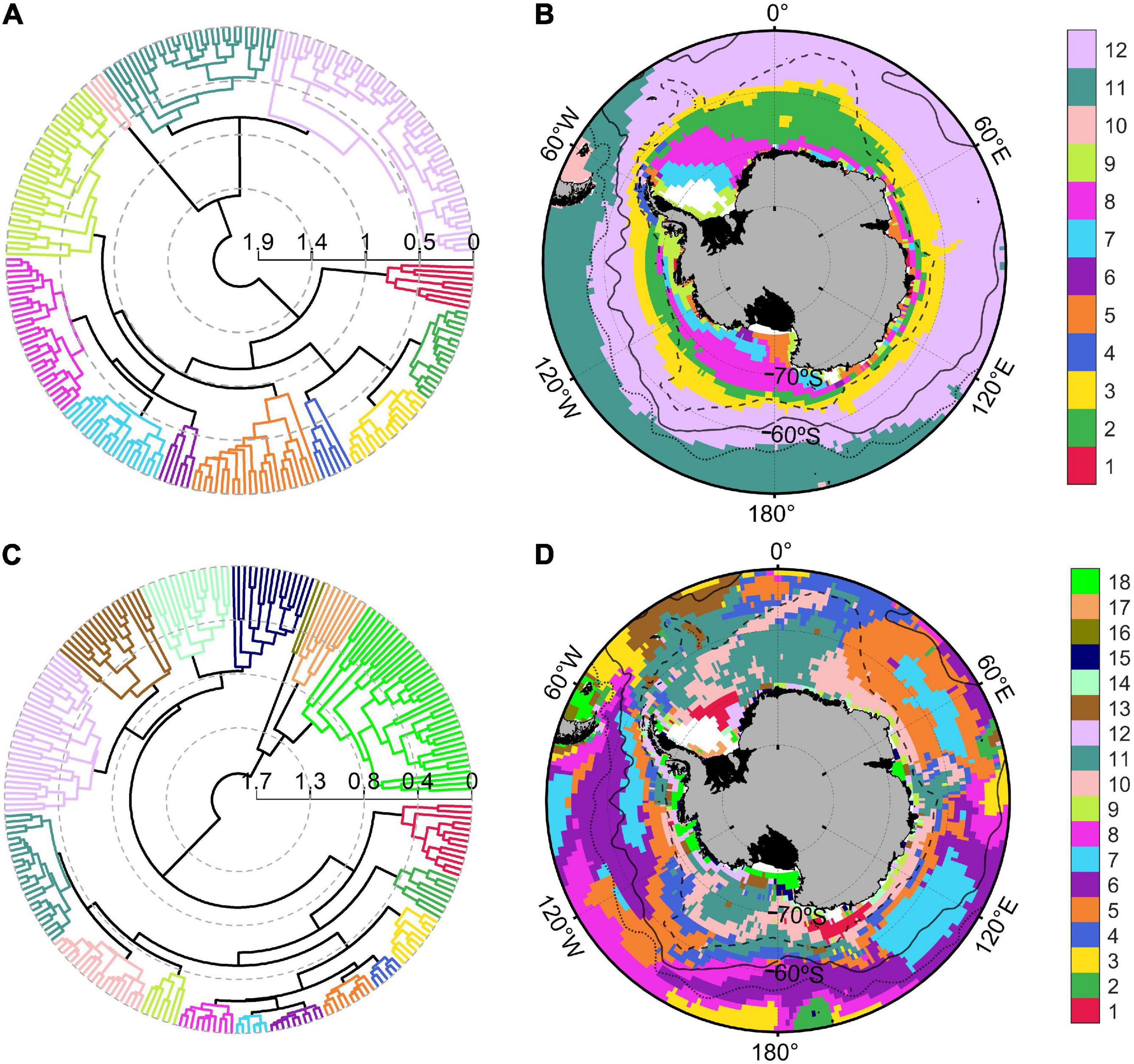
Figure 2. Polar dendrogram and spatial distribution of the clusters obtained from physical (A,B) and biogeochemical (C,D) variables for the Southern Ocean. Black solid, dotted and dashed lines within Southern Ocean map indicated the geographic position of the Polar, Subantarctic and Southern Boundary fronts, respectively.

Biogeochemical Regionalization

The dendrogram of biogeochemical variables (Figure 2C; cophenetic correlation coefficient: 0.78) was divided into 18 significant clusters. Four oceanic groups of the Atlantic, Indian and Pacific sectors (n° 5, 6, 7, and 11; Figure 2D) were characterized by low POC export (ranging from 4.15 to 5.07 mg C m^–2 d^–1), diminished diatoms concentrations (varying between 0.26 and 0.44 mg Chl-a m^–3) and covered approximately 52% of the Southern Ocean surface (Supplementary Table 3). In contrary, coastal Antarctic and Southern Patagonian areas (clusters n° 16, 17, and 18) presented elevated NPP values (ranging from 0.44 to 1.98 g C m^–2 d^–1), diatoms concentrations between 0.55 and 1.06 mg Chl-a m^–3, nanophytoplankton concentrations from 37.85 to 45.45 mg C m^–3 and POC export between 39.90 and 53.06 mg C m^–2 d^–1. Group n° 1 enclosed remote areas from the Weddell Sea (close to the Ronne ice shelf) and the area around the Balleny Islands (near the Ross Sea; Figures 1, 2D), probably because these regions shared the highest dissolved iron concentration in the surface of the Southern Ocean (0.2 nM) and intermediate productivity. The pixels belonging to the Weddell Sea (cluster n° 17) also presented elevated iron concentration, but the productivity and POC export were higher compared with Balleny Islands and Ronne ice shelf (cluster n° 1). The circum-Antarctic pattern identified for oceanic physical regions was less clear during the biogeochemical regionalization. Oceanic island such as South Georgia, Auckland and Kerguelen were grouped in a separate region (n° 2) with much higher POC exports (29.03 mg C m^–2 d^–1) with respect to the oceanic areas of the Indian and Pacific Ocean (n° 6, 7, and 8). The physical properties of the South America coastal region were significantly unique for this zone, whereas the biogeochemical regionalization showed that Southern Patagonia shared biogeochemical properties with coastal Antarctic regions of Ross, Bellingshausen, Amundsen and Cooperation Sea (cluster n°18).

Physical Variables That Explain Biogeochemical Spatial Variability

The latitude showed the highest Pearson linear correlation coefficient (p-value: 0.05) with physical variables (0.77, −0.77, −0.80, and −0.83 for sea ice concentration, SST, MLD, and PAR, respectively; Table 3). On the other hand, the neritic-pelagic gradient seemed to majorly control NPP, diatoms concentration, nanophytoplankton and POC export (with correlation coefficient of 0.55, 0.42, 0.68, and 0.81, respectively), whereas dissolved iron concentration in the photic layer appeared to be mainly controlled by sea-ice dynamics (Pearson linear correlation coefficient: 0.71).

TABLE 3

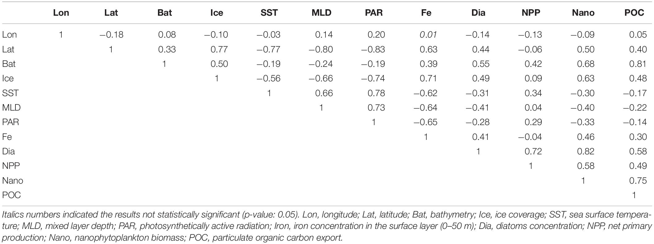
Table 3. Pearson linear correlation coefficient between geographical coordinates, physical and biogeochemical variables within Southern Ocean.

The BIO-ENV analysis identified the combination of bathymetry and sea-ice coverage as the subset of environmental variables with best correlation to biogeochemical spatial variability, with a Spearman rank correlation coefficient of 0.68. Db-RDA (Supplementary Figure 3A) indicated that physical variables expressed the 60.1% of total biogeochemical variance.

CCAMLR Zone 48.1

Physical Regionalization

Important heterogeneity was found in physical variables within the 48.1 CCAMLR zone, with sea ice coverage varying between 0 and 82%, and SST ranging from −0.7 and 3.4°C (Table 2). The agglomerative hierarchical cluster tree for physical variables showed a cophenetic correlation coefficient of 0.78 (Figure 3A), whereas 14 significant clusters were identified. A region with an average sea ice coverage of 3% (n° 5) occupied approximately 33% of the entire 48.1 zone with a southwest (SW)-northeast (NE) distribution that included Shetland Islands (Figure 3B). This cluster presented intermediate depth (mean value: 1,168 m), SST (0.55°C) and MLD (31.8 m) values as compared with other groups (Supplementary Table 4). The SW-NE spatial pattern also appeared for warmer free-ice oceanic clusters located toward the Drake Passage (n° 1, 2, and 4), with the regions n° 2 and 5 that seemed to be separated by the Southern Boundary (Figure 1). The zone of the 48.1 zone closer to the Weddell Sea (clusters n° 9 and 10) exhibited the highest sea ice concentrations (from 64.3 to 69.1%) and coolest waters (between −0.68 and −0.61°C). Marguerite Bay, Gerlache Strait and Crystal Sound (biological hotspots along the Western Antarctic Peninsula; Costa et al., 2007; Figure 1) were clustered into group n° 14, which was characterized by elevated sea ice coverage (mean value: 55%), the shallowest MLD (21 m) and lowest PAR value (20 E m^–2 d^–1) within CCAMLR 48.1 zone. These zones shared physical conditions with the southern part of the Eastern Antarctic Peninsula shelf. Finally, one singleton cluster (n° 6) was observed in the northern tip of Antarctic Peninsula.

FIGURE 3

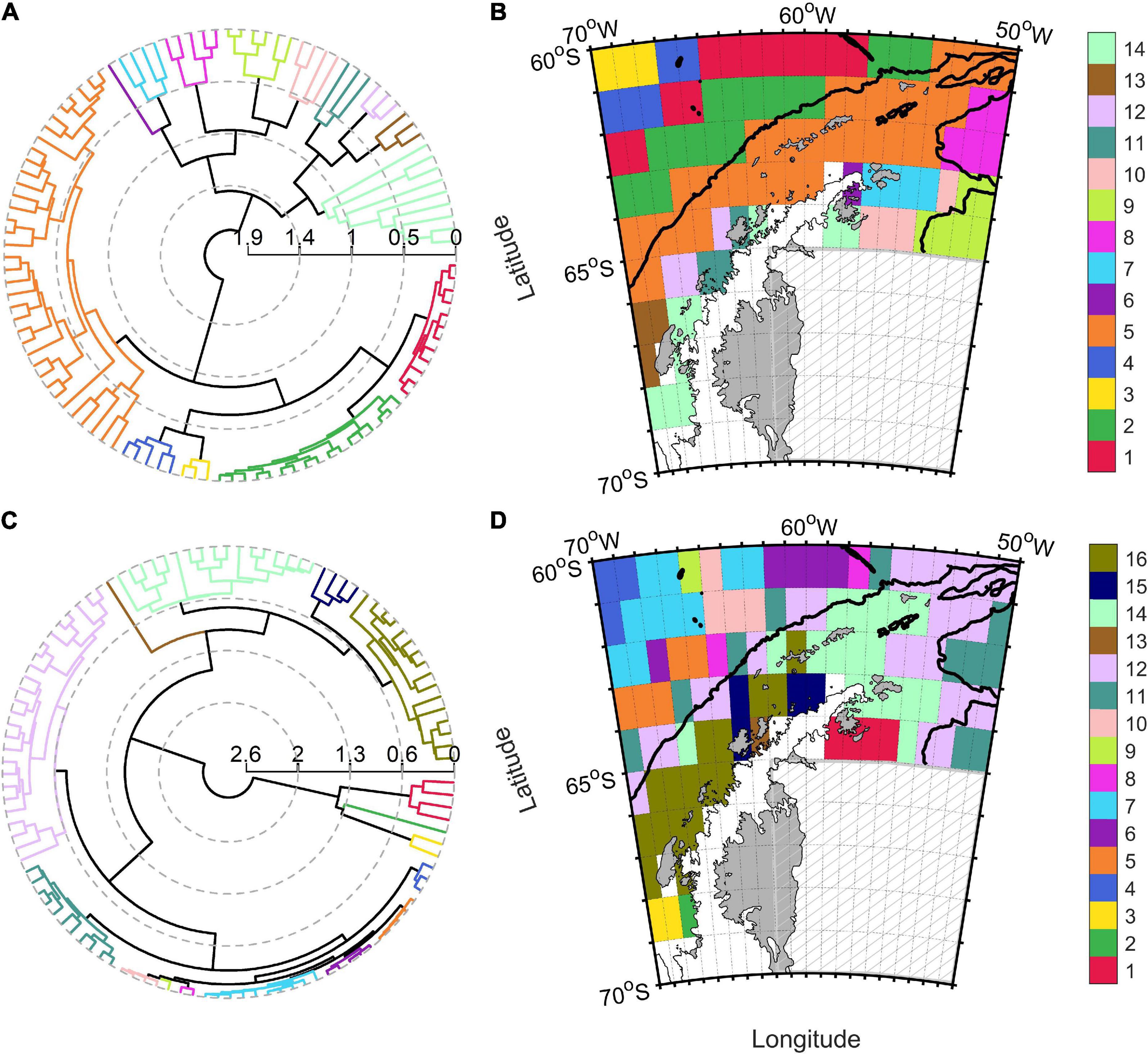
Figure 3. Polar dendrogram and spatial distribution of the clusters obtained from physical (A,B) and biogeochemical (C,D) variables for the CCAMLR 48.1 zone. The black continuous line within 48.1 map indicated the 2,000 m isobath, whereas the gray hatched area represented the zone not included within the CCAMLR 48.1 zone.

Biogeochemical Regionalization

We identified 16 significant clusters within the dendrogram of biogeochemical variables (Figure 3C; cophenetic correlation coefficient: 0.84). Gerlache Strait, the eastern part of Marguerite Bay and one oceanic pixel were identified as singleton biogeochemical clusters (n° 2, 9, and 13) in the CCAMLR zone 48.1 (Figure 3D). Marguerite Bay, the coastal zone of the Eastern Antarctic Peninsula and the area around Crystal Sound (clusters n° 1, 2, 3, and 16) were the most productive clusters in terms of NPP, diatoms, nanophytoplankton concentrations and POC exports (Supplementary Table 5). Conversely, the oceanic region off the Western Antarctic Peninsula (clusters from n° 4 to 10) were the most oligotrophic and presented the least POC export within the 48.1 zone. Pixels belonging to group n° 12 appeared to accurately follow the continental shelf slope and the southern Antarctic Circumpolar Current boundary along the Western Antarctic Peninsula (Moffat and Meredith, 2018). The division marked by the Southern Boundary in physical regionalization appeared less evident in the biogeochemical, whereas a separation between the eastern (n° 14) and western part (n° 15 and 16) of the Bransfield Strait was found (Figure 3D). The similarity between Marguerite Bay and the southern shelf of the Eastern Antarctic Peninsula physical conditions was also observed in the biogeochemical properties (n°1, 2, and 3).

Physical Variables That Explain Biogeochemical Spatial Variability

The longitudinal gradient in CCAMLR zone had a stronger influence in sea ice concentration and SST (Table 4) as compared with the results of the entire Southern Ocean (Table 3). On the other hand, the latitudinal gradient strongly influenced both physical (especially MLD and PAR, with −0.81 and −0.87, respectively) and biogeochemical properties in 48.1 zone (NPP and nanophytoplankton concentrations). Pearson linear correlation coefficient suggested that bathymetry was the main physical factor affecting biogeochemical properties as iron (0.65), POC export (0.96) and diatoms concentrations (0.77; Table 4).

TABLE 4

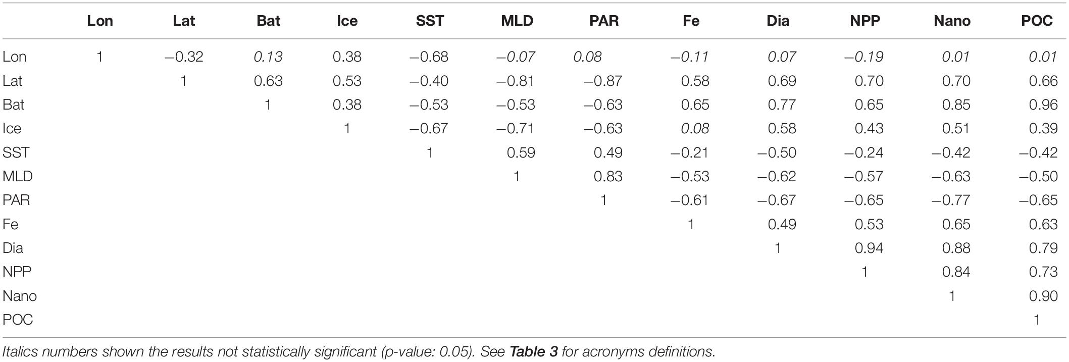
Table 4. Pearson linear correlation coefficient between geographical coordinates, physical and biogeochemical variables within CCAMLR 48.1 zone.

Indeed, BIO-ENV analysis indicated bathymetry as the physical variable with higher correlation to biogeochemical spatial variability (Spearman rank correlation coefficient: 0.81). Additionally, db-RDA (Supplementary Figure 3B) showed that physical variables explained the 77.1% of biogeochemical variance.

Physical and Biogeochemical Regionalization Correspondence

The pixels of each Southern Ocean biogeochemical region belonged on average to 6 different physical zones (± a 95% confidence interval of ±1.5), whereas each physical region was divided in 9 ± 1.4 biogeochemical zones (Figures 4A,B). However, by filtering the results it was calculated that every biogeochemical (physical) region of Southern Ocean averagely corresponded to 1.8 ± 0.2 different physical (biogeochemical) zones. On the contrary, the correspondence degree between biogeochemical and physical regions was higher for CCAMLR 48.1 zone compared with the entire Southern Ocean, since the pixels of each biogeochemical (physical) region on average belonged to 2.3 ± 0.7 (2.7 ± 0.9) physical (biogeochemical) regions (Figures 4C,D). The results decreased to 1.5 ± 0.3 and 1.7 ± 0.4, respectively, when only the pixels that represented more than 20% of total pixels of the corresponding region were considered.

FIGURE 4

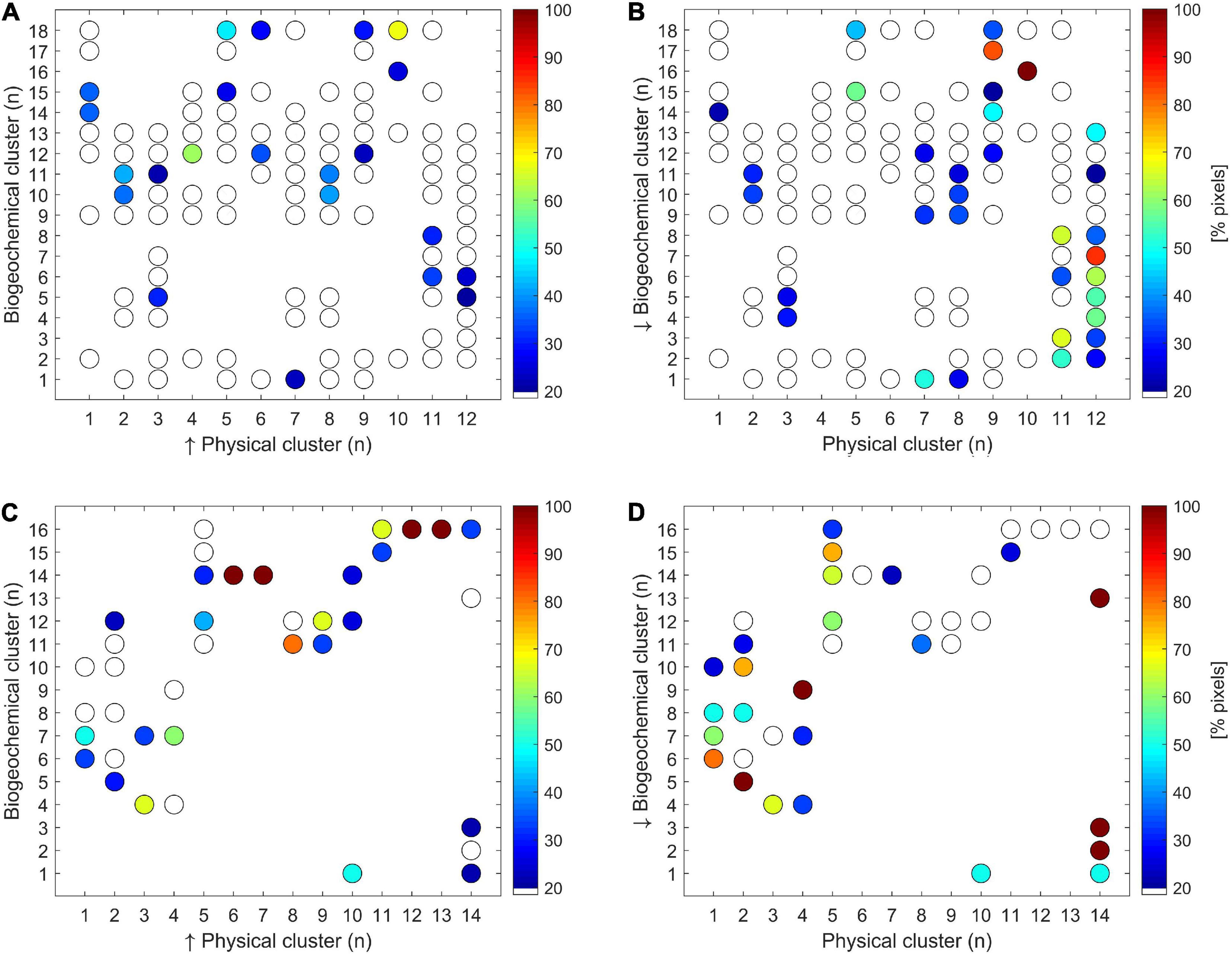
Figure 4. Correspondence (expressed as% of pixels) between physical and biogeochemical clusters within Southern Ocean (A,B) and CCAMLR 48.1 zone (C,D). The white (colored) dots represent the clusters that cover less (more) of 20%. Panels (A,C) show the pixels distribution for every physical cluster within the biogeochemical clusters, whereas panels (B,D) indicated the pixels distribution for every biogeochemical cluster within the physical clusters.

Discussion

Comparison Between Physical and Biogeochemical Regionalization

This study allowed the identification of new physical and biogeochemical regions within the Southern Ocean, enabled the comparison with previous regionalization and provided more explanatory information with respect to other studies. In addition, setting the northern limits at 50°S enabled the creation of new clusters and the study of similarities and differences between Antarctic and Southern Patagonian environments.

Cluster analysis revealed a higher number of significant biogeochemical regions with respect to physical zones. The number of Southern Ocean regions identified in the present work (12 and 18 for physical and biogeochemical variables, respectively) was comparable with other studies of bioregionalization. Indeed, the study of Grant et al. (2006) divided Southern Ocean in 14 different regions based on bathymetry, SST and nutrients concentration, whereas 20 regions were established by Raymond (2014) using bathymetry, SST and ice coverage. Instead, the study of regionalization for CCAMLR 48.1 zone is the first of our knowledge and identifies a surprisingly high number of significant zones (14 physical and 16 biogeochemical regions), probably due to absence of a priori non-hierarchical grouping. The observed circumpolar distribution of physical oceanic clusters marked by the oceanic fronts pattern was similar with the findings of previous regionalization studies (Grant et al., 2006; Spalding et al., 2012; Raymond, 2014). Additionally, Falkland Islands and the coastal zone of the Southern Patagonian were grouped into one physical cluster, which was in agreement with previous works. This work divided the Antarctic coastal area in seven different clusters, which coincided with Raymond (2014) and differed with the regionalization of Grant et al. (2006) that grouped the entire Antarctic coastal area into one region. Grant et al. (2006) additionally identified a separated cluster for the oceanic area of the Weddell gyre, in contrast with the division of this area into four different regions shown by this research and supported by the results of Raymond (2014). The inclusion of sea ice spatial variability into the regionalization variables (Raymond, 2014; this study) might originate higher physical heterogeneity with respect to a regionalization (Grant et al., 2006) that incorporated nitrate and silicate concentrations, since elevated and homogenous macronutrient concentrations are generally observed south of the Southern Boundary and along the Antarctic coastal area (Pollard et al., 2006; Sigman and Hain, 2012).

As expected, the Subantarctic and the Polar Fronts spatial variability influenced the Southern Ocean physical regionalization generating circum-Antarctic clustering (Figure 2B). On the contrary, the spatial variability of oceanic fronts was not reflected in biogeochemical regionalization (Figure 2D), since biogeochemical regions were identified crossing the oceanic fronts in the Indian and Pacific Ocean. In fact, the distinction was not reflected in NPP and phytoplanktonic groups distribution despite the clear difference in SST and MLD at both sides of the fronts (Supplementary Figure 1). Low NPP estimations might be explained by a combination of light limitation (Venables and Moore, 2010), zooplankton grazing (Le Quéré et al., 2016) and dissolved iron depletion (Tagliabue et al., 2014; Wadley et al., 2014).

The coastal zones around South America and Falkland Islands were merged into one physical cluster significantly different from all others in the Southern Ocean (Figure 2B). Contrarily, the coastal region around the southern part of Patagonia was divided in two regions according to biogeochemical variables (i.e., 16 and 18) and the cluster n° 18 also appeared near the coastal zone of Ross, Bellingshausen, Amundsen and Cooperation Sea (Figures 1, 2D). This suggested that coastal zones of Patagonia and some Antarctic zones shared common biogeochemical features (high NPP estimations and diatoms concentrations; Supplementary Table 3), but not physical dynamics. The high productivity of coastal Antarctic zones might be fueled by marginal sea-ice melting during austral summer, injecting micronutrients (Lannuzel et al., 2016) and increasing the photic layer stability (Taylor et al., 2013), whereas the high NPP around the southern part of the Patagonia might be sustained by high tidal energy dissipation and mixing above the continental shelf (Romero et al., 2006), continental freshwater discharges (Cuevas et al., 2019) and the possible iron supply by shelf transport (Garcia et al., 2008) or atmospheric dust (Jickells et al., 2005). Future modeling studies might test the influence of physical and chemical factors on primary production and carbon export in Antarctic and Southern Patagonian related biogeochemical zones under different climate change scenarios.

Additionally, Southern Ocean waters surrounding oceanic islands as Auckland, Kerguelen and South Georgia (Figure 1) were grouped in separated biogeochemical clusters (n°2 and 13; Figure 2D), whereas this distinction was not revealed by physical regionalization. The elevated NPP rates (Supplementary Table 3) and the annual bloom around these oceanic islands can be explained by an “island mass effect” primary produced by downstream iron fertilization via advection (Boyd et al., 2004; Robinson et al., 2016). Sediment pore waters of oceanic islands are a key source of iron in the Southern Ocean (Graham et al., 2015), since iron is released into the photic layer via internal waves and mixing (Korb et al., 2008) and can fuel phytoplankton blooms. In spite of this, interannual variability in the magnitude and extension of the island mass effect might also be influenced by macronutrients and light limitation (Robinson et al., 2016).

The spatial distribution of the Southern Boundary and the Polar Front influenced the physical regionalization of the NW zone of the CCAMLR 48.1 region (clusters n° 2 and 5) but this division was not clearly detected in the biogeochemical regionalization (Figures 1, 3). On the other hand, the physical regionalization of the CCAMLR 48.1 zone didn’t identified a difference between the eastern and western parts of the Bransfield Strait which, on the contrary, was observed in the biogeochemical regionalization (Figure 3). Intense continental meltwater input and the influence of the Antarctic Slope Current (Figure 1) that brings waters from the Weddell Sea (Sangrà et al., 2011; Moffat and Meredith, 2018) might cause the biogeochemical division between the western and eastern part of the Bransfield Strait. Marguerite Bay and the southern shelf of the Eastern Antarctic Peninsula presented similar physical and biogeochemical conditions, with the shallowest MLD and highest NPP estimations and diatoms concentrations, probably due to the elevated presence of sea ice during the austral summer and its influence on biogeochemical cycles (Hyatt et al., 2011; Siegert et al., 2019).

No strong consistency was observed between the physical and biogeochemical regionalization of the Southern Ocean (Figure 4), whereas this correlation was higher for CCAMLR 48.1 zone. The higher consistency between physical and biogeochemical regionalization for 48.1 zone might be explained by either the reduced sample size and/or the response of both biogeochemical and physical regions to the spatial patterns of the shelf slope (Figure 3), as also pointed out by Heywood et al. (2014). The inconsistency detected for the Southern Ocean might be ascribed to the lower spatial variability of biogeochemical variables explained by physical factors as compared with the CCAMLR 48.1 area (60 and 77%, respectively). Indeed, Southern Ocean regions with different physical conditions might present the same biogeochemical features (and High Nutrient Low Chlorophyll patterns), as resulted from oceanic areas around the Subantarctic and the Polar Fronts (Figures 2B–D). This difference might induce a more comparable number of physical and biogeochemical clusters for CCAMLR 48.1 zone (14 and 16, respectively) with respect to the Southern Ocean (12 and 18).

Neither physical nor biogeochemical Southern Ocean regionalization identified a separated cluster for CCAMLR 48.1 zone. Indeed, the limits of the CCAMLR zone included heterogeneous zones with coastal and open water areas, islands, as well as areas belonging to either the Western or Eastern part of the Antarctic Peninsula. This heterogeneity was reflected in elevated number of biogeochemical and physical clusters within CCAMLR 48.1 zone, suggesting that the 48.1 limits were identified exclusively for statistical purposes¹¹ and should be revised following biogeochemical criteria.

Main Physical Factors Explaining Biogeochemical Spatial Variability

BIO-ENV analysis revealed that the combination of bathymetry and sea-ice concentration majorly controlled the biogeochemical spatial variability in the Southern Ocean. Both the neritic-pelagic gradient and sea ice variability affect nutrients and iron cycles and stoichiometry (Garcia et al., 2008; Torres et al., 2014; Annett et al., 2017; Cuevas et al., 2019; Henley et al., 2020), water column stability (Hellmer, 2004; Romero et al., 2006; Cuevas et al., 2019) and irradiance balance (Smith Jr. and Comiso, 2008). In addition, bathymetry directly affects the POC oxygen exposure time to remineralization (Dunne et al., 2007), whereas high pulses of krill fecal pellets that strongly contribute to POC exports (Henley et al., 2020) have been discovered near the marginal ice zone (Belcher et al., 2019). As a result, sea ice variability is a sensible mechanism able to influence NPP rates, POC exports and phytoplankton species composition (Deppeler and Davidson, 2017). Changes in dissolved iron supply, light availability, stratification and ice-free period are projected to affect the biogeochemical cycles and increase Southern Ocean NPP rates up to 50%, in contrast with global trend of declining NPP (Henley et al., 2020). Sea ice variability also influence the production of dimethyl sulfide, a climate-active gas with high concentration in the marginal ice zone (Meredith et al., 2017; Hendry et al., 2018; Henley et al., 2019), and plays an important role in controlling the amount of organic matter that reaches the benthic community (Hendry et al., 2018; Henley et al., 2019). The strong interdependency between sea ice and phytoplankton abundance and size spectrum implies that its variability is also able to alter higher trophic levels of the food web, changing the structure and functioning of the entire ecosystem (Kerr et al., 2018). Indeed, a reduction in sea ice coverage and a shift from a cold and dry climate toward maritime conditions might disadvantage some species (such as Adélie penguins, Weddell seals and minke whales) and favor others (e.g., gentoo penguins and humpback whales; Henley et al., 2019 and references therein).

Bathymetry was identified as the physical variable that majorly described the biogeochemical spatial variability in the CCAMLR 48.1 zone, contrarily to the Southern Ocean where the combination of bathymetry and sea ice was established as the main feature controlling biogeochemical variability. The exclusion of sea ice variability in the 48.1 area might be ascribed to the low spatial heterogeneity in sea ice concentration during the austral summer, since most of the Antarctic Peninsula exhibited low sea ice concentrations with exception of Marguerite Bay and the southern part of the Eastern Antarctic Peninsula (Supplementary Figure 2).

The number and extension of biogeochemical regions might be affected by future variability since both sea ice and bathymetry will experiment changes (on different time scale). Indeed, changes in continental shelf width and bathymetry might occur on decadal to century time scales because of the balance between glacial isostatic adjustment (+41 mm yr^–1; Barletta et al., 2018) and sea level rise (+1.2 mm yr^–1; King et al., 2012). The spatial variability of sea ice trends for the Southern Ocean during 40 years (from 1978 to 2018; Figure 5) showed significant heterogenous trends along the major Antarctic marginal sea ice zones and the CCAMLR 48.1 zone, mainly explained by surface atmospheric circulation patterns (Eayrs et al., 2019) and deep ocean warming (Meredith et al., 2017). Despite the negative sea ice trend detected in the Western Antarctic Peninsula since 1978, a hiatus in atmospheric temperature and sea ice trend has been recorded in this area during the last two decades as part of the natural interdecadal climate variability (Meredith et al., 2017; Henley et al., 2019). Parkinson (2019) shown that sea ice coverage trends were reversed during the 2014–2018 period with sea ice loss in the Weddell and Ross Sea and in the Indian and Western Pacific Ocean; whereas a sea ice gain was observed for the Bellingshausen and Amundsen Sea. These opposite sea ice trends were mainly explained by the combination of atmospheric events (El Niño-Southern Oscillation, the Southern Annular Mode fluctuations and regional circulation flows) and oceanic variability (subsurface heat anomalies and polynyas creation; Parkinson, 2019; Turner et al., 2020). Oceanic biogeochemical regions of the Southern Ocean might also be affected by climate variability, since a poleward expansion of subantarctic waters and a contraction in biogeochemical regions closer to the Antarctic continent were projected for 2100 (Reygondeau et al., 2020).

FIGURE 5

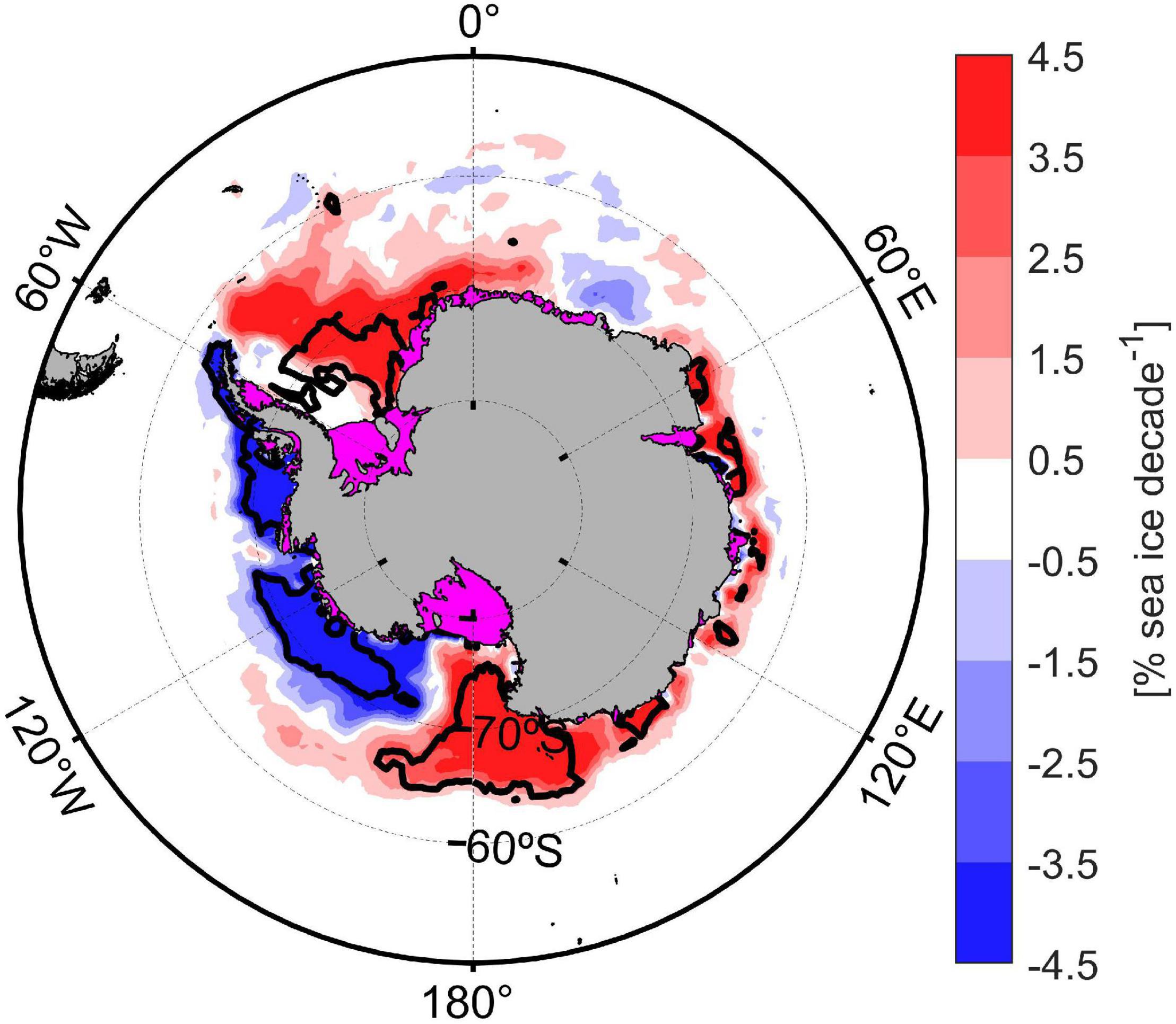
Figure 5. Sea-ice coverage spatial trend during the last 40 years (1978–2018). Black contour line indicated zones with a significant trend (p-value: 0.05).

Future Challenges

This work provides useful information for future parametrization and calibration of biogeochemical models for both the Southern Ocean and the 48.1 zone. Further subjective clustering methods might allow the identification of macro physical and biogeochemical provinces (Spalding et al., 2012) in the Southern Ocean in order to facilitate modeling purposes. The results of the biogeochemical regionalization suggested the division of the 48.1 zone in two provinces (the region above the continental shelf and the deeper ocean) for future ecosystem parametrizations. The study additionally suggests the exclusion of the northerner part of the Eastern Antarctic Peninsula and Marguerite Bay during the parametrization of the 48.1 zone because the physical and biogeochemical dynamics seemed to be strongly affected by either higher presence of sea ice for Marguerite Bay (Hyatt et al., 2011; Siegert et al., 2019; Figure 1) or inflow from Weddell Sea in the Eastern Antarctic Peninsula (Moffat and Meredith, 2018).

This study identified the most productive biogeochemical regions for both the Southern Ocean and CCMAR 48.1 zone. This valuable information will be useful in the development and support of marine protected area proposals, although additional information, such as the spatial variability of higher trophic levels (i.e., zooplankton, zoobenthos, fish, birds, and marine mammals), is needed to create a more solid proposition. The biogeochemical regionalization was initially designed with the inclusion of intermediate trophic levels (i.e., zooplankton abundances). Unfortunately, even the largest Euphausia superba and Salpa thompsoni abundance database for the Southern Ocean (i.e., KRILLBASE; Atkinson et al., 2017) presented extended regions with missing data (Supplementary Figures 4A,B). A continuous updating of krill and salp abundance databases within the Southern Ocean is a must, in order to develop detailed studies regarding food web spatial variability. Abundance data of copepods such as Calanoides acutus and Rhincalanus gigas were even sparser in the Southern Ocean (Supplementary Figures 4C,D), despite of merging the Coastal and Oceanic Plankton Ecology, Production, and Observation Database¹², the Southern Ocean Continuous Plankton Record database¹³ and the database provided by Cornils et al. (2018). The summary and standardization of published copepods data within a new Southern Ocean database is considered an important challenge ahead for the scientific community. A regionalization for 48.1 zone including zooplankton abundances is also needed in the near future in order to develop and improve ecosystem management, such as regulation of fisheries, tourism, contamination and creation of marine and terrestrial protected areas and sanctuaries.

The dataset containing the gridded mean value for physical and biogeochemical variables from December to March within the entire Southern Ocean will be shared with colleagues, consistent with the principle of free-access data and analysis in order to face the actual social and climate crisis.

Conclusion

This regionalization study allowed the identification of new regions within the Southern Ocean and comparisons with previous regionalization developed using physical and biogeochemical variables. The number of the physical and biogeochemical Southern Ocean regions identified in this study (12 and 18, respectively) was comparable with previous studies of bioregionalization. However, southern Patagonian coastal areas were merged into a physical cluster significantly different from all others in the Southern Ocean, whereas biogeochemical patterns were shared with coastal Antarctic areas (i.e., Ross, Bellingshausen, Amundsen, and Cooperation Sea). The combination of bathymetry and sea ice coverage majorly explained biogeochemical variability within the Southern Ocean (Spearman rank correlation coefficient: 0.68). Since both sea ice and bathymetry will experiment changes, although on different time scale, our results suggest the number and extension of biogeochemical regions might be affected in the future.

Fourteen physical and 16 biogeochemical significant clusters were identified for 48.1 CCAMLR zone, where bathymetry was the main factor explaining biogeochemical spatial variability (0.81). The results suggested the division of the 48.1 zone in two main provinces separated by the shelf slope during future ecosystem parametrizations, with the exclusion of the northerner part of the Eastern Antarctic Peninsula and Marguerite Bay, because those regions were affected by either higher presence of sea ice (for Marguerite Bay) or inflow from Weddell Sea (in the Eastern Antarctic Peninsula).

The correspondence between physical and biogeochemical regions was higher for CCAMLR 48.1 zone with respect to the entire Southern Ocean, probably ascribed to the lower spatial variability of biogeochemical variables explained by physical factors in the Southern Ocean as compared with the CCAMLR 48.1 area (60 and 77%, respectively). Both physical and biogeochemical Southern Ocean regionalization failed to identify a separated cluster for CCAMLR 48.1 zone, suggesting that the 48.1 limits should be revised following biogeochemical criteria.

This study provides useful data for both Southern Ocean and CCAMLR 48.1 zone management and ecosystem parametrization purposes.

Data Availability Statement

The original contributions presented in the study are included in the article/Supplementary Material, further inquiries can be directed to the corresponding author.

Author Contributions

GT, AP, and LC analyzed the data and wrote the manuscript. All authors contributed to the article and approved the submitted version.

Funding

This study was supported by FONDECYT 11170913, FONDAP 15150003, National Agency for Research and Development (ANID)/PFCHA/Doctorado Nacional/2017-21170561, and COPAS Sur Austral ANID PIA Apoyo CCTE AFB 170006.

Conflict of Interest

The authors declare that the research was conducted in the absence of any commercial or financial relationships that could be construed as a potential conflict of interest.

Acknowledgments

We thank R. Giesecke, S. Neira, the associate editor, and reviewers for their valuable comments and suggestions.

Supplementary Material

The Supplementary Material for this article can be found online at: https://www.frontiersin.org/articles/10.3389/fmars.2021.592378/full#supplementary-material

Footnotes

1. ^ http://www.soos.aq/activities/rwg/wapsa
2. ^ https://catalog.data.gov/dataset
3. ^ https://www.metoffice.gov.uk/hadobs
4. ^ https://coastwatch.pfeg.noaa.gov/
5. ^ http://sose.ucsd.edu
6. ^ http://sites.science.oregonstate.edu/ocean.productivity/
7. ^ https://www.pangaea.de/
8. ^ https://data.aad.gov.au/
9. ^ https://cran.r-project.org/
10. ^ https://mathworks.com/
11. ^ https://www.ccamlr.org/en/organisation/explanation-terms
12. ^ https://www.st.nmfs.noaa.gov/copepod/
13. ^ https://www.scar.org/science/cpr/

References

Ainley, D. G., and Pauly, D. (2014). Fishing down the food web of the Antarctic continental shelf and slope. Polar Rec. 50, 92–107. doi: 10.1017/S0032247412000757

CrossRef Full Text | Google Scholar

Annett, A. L., Fitzsimmons, J. N., Séguret, M. J. M., Lagerström, M., Meredith, M. P., Schofield, O., et al. (2017). Controls on dissolved and particulate iron distributions in surface waters of the Western Antarctic Peninsula shelf. Mar. Chem. 196, 81–97. doi: 10.1016/j.marchem.2017.06.004

CrossRef Full Text | Google Scholar

Armitage, T. W. K., Kwok, R., Thompson, A. F., and Cunningham, G. (2018). Dynamic Topography and Sea Level Anomalies of the Southern Ocean: Variability and Teleconnections. J. Geophys. Res. Ocean. 123, 613–630. doi: 10.1002/2017JC013534

CrossRef Full Text | Google Scholar

Atkinson, A., Hill, S. L., Pakhomov, E. A., Siegel, V., Anadon, R., Chiba, S., et al. (2017). KRILLBASE: A circumpolar database of Antarctic krill and salp numerical densities, 1926-2016. Earth Syst. Sci. Data 9, 193–210. doi: 10.5194/essd-9-193-2017

CrossRef Full Text | Google Scholar

Bargagli, R. (2008). Environmental contamination in Antarctic ecosystems. Sci. Total Environ. 400, 212–226. doi: 10.1016/j.scitotenv.2008.06.062

PubMed Abstract | CrossRef Full Text | Google Scholar

Barletta, V. R., Bevis, M., Smith, B. E., Wilson, T., Brown, A., Bordoni, A., et al. (2018). Observed rapid bedrock uplift in Amundsen Sea Embayment promotes ice-sheet stability. Science 360, 1335–1339. doi: 10.1126/science.aao1447

PubMed Abstract | CrossRef Full Text | Google Scholar

Behrenfeld, M. J., and Falkowski, P. G. (1997). Photosynthetic rates derived from satellite-based chlorophyll concentration. Limnol. Oceanogr. 42, 1–20. doi: 10.4319/lo.1997.42.1.0001

CrossRef Full Text | Google Scholar

Belcher, A., Henson, S. A., Manno, C., Hill, S. L., Atkinson, A., Thorpe, S. E., et al. (2019). Krill faecal pellets drive hidden pulses of particulate organic carbon in the marginal ice zone. Nat. Commun. 10:889. doi: 10.1038/s41467-019-08847-1

PubMed Abstract | CrossRef Full Text | Google Scholar

Berline, L. O., Rammou, A. M., Doglioli, A., Molcard, A., and Petrenko, A. (2014). A connectivity-based Eco-regionalization method of the Mediterranean Sea. PLoS One 9:e111978. doi: 10.1371/journal.pone.0111978

PubMed Abstract | CrossRef Full Text | Google Scholar

Borcard, D., Gillet, F., and Legendre, P. (2018). Numerical Ecology with R. New York, NY: Springer, doi: 10.1007/978-3-319-71404-2

CrossRef Full Text | Google Scholar

Boyd, P. W., McTainsh, G., Sherlock, V., Richardson, K., Nichol, S., Ellwood, M., et al. (2004). Episodic enhancement of phytoplankton stocks in New Zealand subantarctic waters: Contribution of atmospheric and oceanic iron supply. Global Biogeochem. Cycles 18:GB1029. doi: 10.1029/2002gb002020

CrossRef Full Text | Google Scholar

Boyd, P. W., Jickells, T., Law, C. S., Blain, S., Boyle, E. A., Buesseler, K. O., et al. (2007). Mesoscale iron enrichment experiments 1993-2005: Synthesis and future directions. Science 315, 612–617. doi: 10.1126/science.1131669

PubMed Abstract | CrossRef Full Text | Google Scholar

Boyd, I. L. (2009). “Antarctic Marine Mammals,” in Encyclopedia of Marine Mammals (Second Edition), eds W. F. Perrin, B. Würsig, and J. G. M. Thewissen (Cambridge, MA: Academic Press), 42–46. doi: 10.1016/B978-0-12-804327-1.00047-9

CrossRef Full Text | Google Scholar

Brooks, C. M., Ainley, D. G., Abrams, P. A., Dayton, P. K., Hofman, R. J., Jacquet, J., et al. (2018). Watch over antarctic waters. Nature 558, 177–180. doi: 10.1038/d41586-018-05372-x

PubMed Abstract | CrossRef Full Text | Google Scholar

Cabré, A., Shields, D., Marinov, I., and Kostadinov, T. S. (2016). Phenology of Size-Partitioned Phytoplankton Carbon-Biomass from Ocean Color Remote Sensing and CMIP5 Models. Front. Mar. Sci. 3:39. doi: 10.3389/fmars.2016.00039

CrossRef Full Text | Google Scholar

CCAMLR (2018). Statistical Bulletin. Volume 30. Commission for the Conservation of Antarctic Marine Living Resources. Australia: CCAMLR.

Google Scholar

Charrad, M., Ghazzali, N., Boiteau, V., and Niknafs, A. (2014). Nbclust: An R package for determining the relevant number of clusters in a data set. J. Stat. Softw. 61, 1–36. doi: 10.18637/jss.v061.i06

CrossRef Full Text | Google Scholar

Clarke, K. R., and Ainsworth, M. (1993). A method of linking multivariate community structure to environmental variables. Mar. Ecol. Prog. Ser. 92, 205–219. doi: 10.3354/meps092205

CrossRef Full Text | Google Scholar

Clarke, K. R., Somerfield, P. J., and Gorley, R. N. (2008). Testing of null hypotheses in exploratory community analyses: similarity profiles and biota-environment linkage. J. Exp. Mar. Bio. Ecol. 366, 56–69. doi: 10.1016/j.jembe.2008.07.009

CrossRef Full Text | Google Scholar

Comiso, J. C., Gersten, R. A., Stock, L. V., Turner, J., Perez, G. J., and Cho, K. (2017). Positive trend in the Antarctic sea ice cover and associated changes in surface temperature. J. Clim. 30, 2251–2267. doi: 10.1175/JCLI-D-16-0408.1

PubMed Abstract | CrossRef Full Text | Google Scholar

Cornils, A., Sieger, R., Mizdalski, E., Schumacher, S., Grobe, H., and Schnack-Schiel, S. B. (2018). Copepod species abundance from the Southern Ocean and other regions (1980-2005) - A legacy. Earth Syst.Sci. Data 10, 1457–1471. doi: 10.5194/essd-10-1457-2018

CrossRef Full Text | Google Scholar

Costa, D. P., Burns, J. M., Chapman, E., Hildebrand, J., Torres, J. J., Fraser, W., et al. (2007). US SO GLOBEC Predator Programme. GLOBEC Int. Newsletter 13, 62–66.

Google Scholar

Cuevas, L. A., Tapia, F. J., Iriarte, J. L., González, H. E., Silva, N., and Vargas, C. A. (2019). Interplay between freshwater discharge and oceanic waters modulates phytoplankton size-structure in fjords and channel systems of the Chilean Patagonia. Prog. Oceanogr. 173, 103–113. doi: 10.1016/j.pocean.2019.02.012

CrossRef Full Text | Google Scholar

David, B., and Saucède, T. (2015). Southern Ocean Biogeography and Communities in The Southern Ocean. Amsterdam: Elsevier, 43–57. doi: 10.1016/b978-1-78548-047-8.50004-7

CrossRef Full Text | Google Scholar

Deppeler, S. L., and Davidson, A. T. (2017). Southern Ocean phytoplankton in a changing climate. Front. Mar. Sci. 4:40. doi: 10.3389/fmars.2017.00040

CrossRef Full Text | Google Scholar

Douglass, L. L., Turner, J., Grantham, H. S., Kaiser, S., Constable, A., Nicoll, R., et al. (2014). A hierarchical classification of benthic biodiversity and assessment of protected areas in the Southern Ocean. PLoS One 9:e100551. doi: 10.1371/journal.pone.0100551

PubMed Abstract | CrossRef Full Text | Google Scholar

Dunne, J. P., Sarmiento, J. L., and Gnanadesikan, A. (2007). A synthesis of global particle export from the surface ocean and cycling through the ocean interior and on the seafloor. Global Biogeochem. Cycles 21:GB4006. doi: 10.1029/2006GB002907

CrossRef Full Text | Google Scholar

Eayrs, C., Holland, D., Francis, D., Wagner, T., Kumar, R., and Li, X. (2019). Understanding the Seasonal Cycle of Antarctic Sea Ice Extent in the Context of Longer-Term Variability. Rev. Geophys. 57, 1037–1064. doi: 10.1029/2018RG000631

CrossRef Full Text | Google Scholar

Fabri-Ruiz, S., Danis, B., Navarro, N., Koubbi, P., Laffont, R., and Saucède, T. (2020). Benthic ecoregionalization based on echinoid fauna of the Southern Ocean supports current proposals of Antarctic Marine Protected Areas under IPCC scenarios of climate change. Glob. Chang. Biol. 26, 2161–2180. doi: 10.1111/gcb.14988

PubMed Abstract | CrossRef Full Text | Google Scholar

FAO (2018). The State of World Fisheries and Aquaculture 2018 - Meeting the sustainable development goals. Food and Agriculture Organization.

Google Scholar

Garcia, V. M. T., Garcia, C. A. E., Mata, M. M., Pollery, R. C., Piola, A. R., Signorini, S. R., et al. (2008). Environmental factors controlling the phytoplankton blooms at the Patagonia shelf-break in spring. Deep. Res. Part I Oceanogr. Res. Pap. 55, 1150–1166. doi: 10.1016/j.dsr.2008.04.011

CrossRef Full Text | Google Scholar

Graham, R. M., De Boer, A. M., van Sebille, E., Kohfeld, K. E., and Schlosser, C. (2015). Inferring source regions and supply mechanisms of iron in the Southern Ocean from satellite chlorophyll data. Deep Sea Res. Part I Oceanogr. Res. Pap. 104, 9–25. doi: 10.1016/j.dsr.2015.05.007

CrossRef Full Text | Google Scholar

Grant, S. M., Constable, M., Raymond, B., and Doust, S. (2006). Bioregionalisation of the Southern Ocean: Report of Experts Workshop (Hobart, September 2006). Sydney: WWF-Australia and ACECRC. 44.

Google Scholar

Grant, S. M., Hill, S. L., Trathan, P. N., and Murphy, E. J. (2013). Ecosystem services of the Southern Ocean: trade-offs in decision-making. Antarct. Sci. 25, 603–617. doi: 10.1017/s0954102013000308

PubMed Abstract | CrossRef Full Text | Google Scholar

Griffiths, H. J., Barnes, D. K. A., and Linse, K. (2009). Towards a generalized biogeography of the Southern Ocean benthos. J. Biogeogr. 36, 162–177. doi: 10.1111/j.1365-2699.2008.01979.x

CrossRef Full Text | Google Scholar

Gruber, N., Clement, D., Carter, B. R., Feely, R. A., van Heuven, S., Hoppema, M., et al. (2019). The oceanic sink for anthropogenic CO 2 from 1994 to 2007. Science 363, 1193–1199. doi: 10.1126/science.aau5153

PubMed Abstract | CrossRef Full Text | Google Scholar

Guillaumot, C., Aguera, A., and Danis, B. (2017). Particulate carbon export flux layers.Australia: Australian Antarctic Data Centre. doi: 10.4225/15/58fff5231f00a

CrossRef Full Text | Google Scholar

Hellmer, H. H. (2004). Impact of Antarctic ice shelf basal melting on sea ice and deep ocean properties. Geophys. Res. Lett. 31:L10307. doi: 10.1029/2004GL019506

CrossRef Full Text | Google Scholar

Hendry, K. R., Meredith, M. P., and Ducklow, H. W. (2018). The marine system of the West Antarctic Peninsula: Status and strategy for progress. Philos. Trans. R. Soc. A Math. Phys. Eng. Sci. 376:20170179. doi: 10.1098/rsta.2017.0179

PubMed Abstract | CrossRef Full Text | Google Scholar

Henley, S. F., Schofield, O. M., Hendry, K. R., Schloss, I. R., Steinberg, D. K., Moffat, C., et al. (2019). Variability and change in the west Antarctic Peninsula marine system: Research priorities and opportunities. Prog. Oceanogr. 173, 208–237. doi: 10.1016/j.pocean.2019.03.003

CrossRef Full Text | Google Scholar

Henley, S. F., Cavan, E. L., Fawcett, S. E., Kerr, R., Monteiro, T., Sherrell, R. M., et al. (2020). Changing Biogeochemistry of the Southern Ocean and Its Ecosystem Implications. Front. Mar. Sci. 7:00581. doi: 10.3389/fmars.2020.00581

CrossRef Full Text | Google Scholar

Heywood, K. J., Naveira Garabato, A. C., Stevens, D. P., and Muench, R. D. (2004). On the fate of the Antarctic Slope Front and the origin of the Weddell Front. J. Geophys. Res. C Ocean. 109:C06021. doi: 10.1029/2003JC002053

CrossRef Full Text | Google Scholar

Heywood, K. J., Schmidtko, S., Heuzé, C., Kaiser, J., Jickells, T. D., Queste, B. Y., et al. (2014). Ocean processes at the Antarctic continental slope. Philos. Trans. R. Soc. A Math. Phys. Eng. Sci. 372:20130047. doi: 10.1098/rsta.2013.0047

PubMed Abstract | CrossRef Full Text | Google Scholar

Hogg, O. T., Huvenne, V. A. I., Griffiths, H. J., Dorschel, B., and Linse, K. (2016). Landscape mapping at sub-Antarctic South Georgia provides a protocol for underpinning large-scale marine protected areas. Sci. Rep. 6, 1–15. doi: 10.1038/srep33163

PubMed Abstract | CrossRef Full Text | Google Scholar

Holte, J., Talley, L. D., Gilson, J., and Roemmich, D. (2017). An Argo mixed layer climatology and database. Geophys. Res. Lett. 44, 5618–5626. doi: 10.1002/2017GL073426

CrossRef Full Text | Google Scholar

Hyatt, J., Beardsley, R. C., and Owens, W. B. (2011). Characterization of sea ice cover, motion and dynamics in Marguerite Bay, Antarctic Peninsula. Deep. Res. Part II Top. Stud. Oceanogr. 58, 1553–1568. doi: 10.1016/j.dsr2.2010.08.021

CrossRef Full Text | Google Scholar

IHO (2002). Names and limits of oceans and seas. International Hydrographic Organization. Special Publication n° 23 (4^th ed.). Monaco: International Hydrographic Bureau.

Google Scholar

Jickells, T. D., An, Z. S., Andersen, K. K., Baker, A. R., Bergametti, C., Brooks, N., et al. (2005). Global iron connections between desert dust, ocean biogeochemistry, and climate. Science. 308, 67–71. doi: 10.1126/science.1105959

PubMed Abstract | CrossRef Full Text | Google Scholar

Jones, J. M., Gille, S. T., Goosse, H., Abram, N. J., Canziani, P. O., Charman, D. J., et al. (2016). Assessing recent trends in high-latitude Southern Hemisphere surface climate. Nat. Clim. Chang. 6, 917–926. doi: 10.1038/nclimate3103

CrossRef Full Text | Google Scholar

Kaufman, L., and Rousseeuw, P. J. (1990). Finding groups in data: an introduction to cluster analysis. Hoboken (USA). Hoboken, NJ: Wiley.

Google Scholar

Kerr, R., Mata, M. M., Mendes, C. R. B., and Secchi, E. R. (2018). Northern Antarctic Peninsula: a marine climate hotspot of rapid changes on ecosystems and ocean dynamics. Deep. Res. Part II Top. Stud. Oceanogr. 149, 4–9. doi: 10.1016/j.dsr2.2018.05.006

CrossRef Full Text | Google Scholar

Kindt, R., and Coe, R. (2005). Tree diversity analysis. A manual and software for common statistical methods for ecological and biodiversity studies.

Google Scholar

King, M. A., Bingham, R. J., Moore, P., Whitehouse, P. L., Bentley, M. J., and Milne, G. A. (2012). Lower satellite-gravimetry estimates of Antarctic sea-level contribution. Nature 491, 586–589. doi: 10.1038/nature11621

PubMed Abstract | CrossRef Full Text | Google Scholar

Korb, R. E., Whitehouse, M. J., Atkinson, A., and Thorpe, S. E. (2008). Magnitude and maintenance of the phytoplankton bloom at South Georgia: A naturally iron-replete environment. Mar. Ecol. Prog. Ser. 368, 75–91. doi: 10.3354/meps07525

CrossRef Full Text | Google Scholar

Koshlyakov, M. N., and Tarakanov, R. Y. (2011). Water transport across the subantarctic front and the global ocean conveyer belt. Oceanology 51, 721–735. doi: 10.1134/s0001437011050110

CrossRef Full Text | Google Scholar

Kostadinov, T. S., Milutinovi, S., Marinov, I., and Cabré, A. (2016). Carbon-based phytoplankton size classes retrieved via ocean color estimates of the particle size distribution. Ocean Sci. 12, 561–575. doi: 10.5194/os-12-561-2016

CrossRef Full Text | Google Scholar

Lannuzel, D., Vancoppenolle, M., Van Der Merwe, P., De Jong, J., Meiners, K. M., Grotti, M., et al. (2016). Iron in sea ice: Review & new insights. Elementa 4:000130. doi: 10.12952/journal.elementa.000130

CrossRef Full Text | Google Scholar

Le Quéré, C., Buitenhuis, E. T., Moriarty, R., Alvain, S., Aumont, O., Bopp, L., et al. (2016). Role of zooplankton dynamics for Southern Ocean phytoplankton biomass and global biogeochemical cycles. Biogeosciences 13, 4111–4133. doi: 10.5194/bg-13-4111-2016

CrossRef Full Text | Google Scholar

Legendre, P., and Andersson, M. J. (1999). Distance-based redundancy analysis: Testing multispecies responses in multifactorial ecological experiments. Ecol. Monogr. 69, 1–24. doi: 10.1890/0012-96151999069[0001:DBRATM]2.0.CO;2

CrossRef Full Text | Google Scholar

Li, H., Xu, F., Zhou, W., Wang, D., Wright, J. S., Liu, Z., et al. (2017). Development of a global gridded Argo data set with Barnes successive corrections. J. Geophys. Res. Ocean. 122, 866–889. doi: 10.1002/2016JC012285

CrossRef Full Text | Google Scholar

Lutz, M. J., Caldeira, K., Dunbar, R. B., and Behrenfeld, M. J. (2007). Seasonal rhythms of net primary production and particulate organic carbon flux to depth describe the efficiency of biological pump in the global ocean. J. Geophys. Res. 112:C10011. doi: 10.1029/2006JC003706

CrossRef Full Text | Google Scholar

Martin, J. H., Fitzwater, S. E., and Gordon, R. M. (1990). Iron deficiency limits phytoplankton growth in Antarctic waters. Global Biogeochem Cycles 4, 5–12. doi: 10.1029/GB004i001p00005

CrossRef Full Text | Google Scholar

Mazloff, M. R., Heimbach, P., and Wunsch, C. (2010). An Eddy-Permitting Southern Ocean State Estimate. J. Phys. Oceanogr. 40, 880–899. doi: 10.1175/2009JPO4236.1

CrossRef Full Text | Google Scholar

McBride, M. M., Dalpadado, P., Drinkwater, K. F., Godø, O. R., Hobday, A. J., Hollowed, A. B., et al. (2014). Krill, climate, and contrasting future scenarios for Arctic and Antarctic fisheries. ICES J. Mar. Sci. 71, 1934–1955. doi: 10.1093/icesjms/fsu002

CrossRef Full Text | Google Scholar

Meredith, M. P., Stefels, J., and van Leeuwe, M. (2017). Marine studies at the western Antarctic Peninsula: Priorities, progress and prognosis. Deep. Res. Part II Top. Stud. Oceanogr. 139, 1–8. doi: 10.1016/j.dsr2.2017.02.002

CrossRef Full Text | Google Scholar

Moffat, C., and Meredith, M. (2018). Shelf-ocean exchange and hydrography west of the Antarctic Peninsula: A review. Philos. Trans. R. Soc. A Math. Phys. Eng. Sci. 376:20170164. doi: 10.1098/rsta.2017.0164

PubMed Abstract | CrossRef Full Text | Google Scholar

Morrison, A. K., Frölicher, T. L., and Sarmiento, J. L. (2015). Upwelling in the Southern Ocean. Phys. Today 68, 27–32. doi: 10.1063/pt.3.2654

CrossRef Full Text | Google Scholar

Murphy, E. J., Cavanagh, R. D., Hofmann, E. E., Hill, S. L., Constable, A. J., Costa, D. P., et al. (2012). Developing integrated models of Southern Ocean food webs: Including ecological complexity, accounting for uncertainty and the importance of scale. Prog. Oceanogr. 102, 74–92. doi: 10.1016/j.pocean.2012.03.006

CrossRef Full Text | Google Scholar

Murphy, E. J., Cavanagh, R. D., Drinkwater, K. F., Grant, S. M., Heymans, J. J., Hofmann, E. E., et al. (2016). Understanding the structure and functioning of polar pelagic ecosystems to predict the impacts of change. Proc. R. Soc. B Biol. Sci. 283:20161646. doi: 10.1098/rspb.2016.1646

PubMed Abstract | CrossRef Full Text | Google Scholar

Oksanen, J., Blanchet, F. G., Friendly, M., Kindt, R., Legendre, P., McGlinn, D., et al. (2019). Vegan: Community Ecology Package. R package version 2.5-4. https://CRAN.R-project.org/package=vegan.

Google Scholar

Olson, C. J., Becker, J. J., and Sandwell, D. T. (2016). SRTM15_PLUS: Data fusion of Shuttle Radar Topography Mission (SRTM) land topography with measured and estimated seafloor topography (NCEI Accession 0150537). Version 1.1. Silver Spring: NOAA National Centers for Environmental Information.

Google Scholar

Orsi, A. H., Whitworth, T., and Nowlin, W. D. (1995). On the meridional extent and fronts of the Antarctic Circumpolar Current. Deep. Res. Part I 42, 641–673. doi: 10.1016/0967-0637(95)00021-W

CrossRef Full Text | Google Scholar

Parkinson, C. L. (2019). A 40-y record reveals gradual Antarctic sea ice increases followed by decreases at rates far exceeding the rates seen in the Arctic. Proc. Natl. Acad. Sci. U. S. A. 116, 14414–14423. doi: 10.1073/pnas.1906556116

PubMed Abstract | CrossRef Full Text | Google Scholar

Perry, F. A., Atkinson, A., Sailley, S. F., Tarling, G. A., Hill, S. L., Lucas, C. H., et al. (2019). Habitat partitioning in Antarctic krill: Spawning hotspots and nursery areas. PLoS One 14:e0219325. doi: 10.1371/journal.pone.0219325

PubMed Abstract | CrossRef Full Text | Google Scholar

Pierrat, B., Saucède, T., Brayard, A., and David, B. (2013). Comparative biogeography of echinoids, bivalves and gastropods from the Southern Ocean. J. Biogeogr. 40, 1374–1385. doi: 10.1111/jbi.12088

CrossRef Full Text | Google Scholar

Piñones, A., and Fedorov, A. V. (2016). Projected changes of Antarctic krill habitat by the end of the 21st century. Geophys. Res. Lett. 43, 8580–8589. doi: 10.1002/2016GL069656

CrossRef Full Text | Google Scholar

Pitchford, J. W., and Brindley, J. (1999). Iron limitation, grazing pressure and oceanic high nutrient-low chlorophyll (HNLC) regions. J. Plankton Res. 21, 525–547. doi: 10.1093/plankt/21.3.525

PubMed Abstract | CrossRef Full Text | Google Scholar

Pollard, R., Tréguer, P., and Read, J. (2006). Quantifying nutrient supply to the Southern Ocean. J. Geophys. Res. Ocean. 111:C05011. doi: 10.1029/2005JC003076

CrossRef Full Text | Google Scholar

Raymond, B. (2014). “Chapter 10.2. Pelagic regionalisation,” in Biogeographic Atlas of the Southern Ocean. eds C. De Broyer, P. Koubbi, H. J. Griffiths, B. Raymond, and C. D. Udekem d’Acoz (Cambridge, MA: Scientific Committee on Antarctic Research), 418–421.

Google Scholar

Reid, P. C., Fischer, A. C., Lewis-Brown, E., Meredith, M. P., Sparrow, M., Andersson, A. J., et al. (2009). Impacts of the oceans on climate change. Adv. Mar. Biol. 56, 1–150. doi: 10.1016/S0065-2881(09)56001-4

CrossRef Full Text | Google Scholar

Reygondeau, G., Cheung, W. W. L., Wabnitz, C. C. C., Lam, V. W. Y., Frölicher, T., and Maury, O. (2020). Climate Change-Induced Emergence of Novel Biogeochemical Provinces. Front. Mar. Sci. 7:657. doi: 10.3389/fmars.2020.00657

CrossRef Full Text | Google Scholar

Rintoul, S. R., and da Silva, C. E. (2019). “Antarctic Circumpolar Current,” in Encyclopedia of Ocean Sciences, (Cambridge, MA: Academic Press), 248–261. doi: 10.1016/B978-0-12-409548-9.11298-9

CrossRef Full Text | Google Scholar

Roberts, C. M., O’Leary, B. C., Mccauley, D. J., Cury, P. M., Duarte, C. M., Lubchenco, J., et al. (2017). Marine reserves can mitigate and promote adaptation to climate change. Proc. Natl. Acad. Sci. U. S. A. 114, 6167–6175. doi: 10.1073/pnas.1701262114

PubMed Abstract | CrossRef Full Text | Google Scholar

Robinson, J., Popova, E. E., Srokosz, M. A., and Yool, A. (2016). A tale of three islands: Downstream natural iron fertilization in the Southern Ocean. J. Geophys. Res. Ocean. 121, 3350–3371. doi: 10.1002/2015JC011319

CrossRef Full Text | Google Scholar

Romero, S. I., Piola, A. R., Charo, M., and Eiras Garcia, C. A. (2006). Chlorophyll-a variability off Patagonia based on SeaWiFS data. J. Geophys. Res. Ocean. 111:C05021. doi: 10.1029/2005JC003244

CrossRef Full Text | Google Scholar

Sallée, J. B., Speer, K., and Morrow, R. (2008). Response of the antarctic circumpolar current to atmospheric variability. J. Clim. 21, 3020–3039. doi: 10.1175/2007JCLI1702.1

CrossRef Full Text | Google Scholar

Sallée, J. B. (2018). Southern ocean warming. Oceanography 31, 52–62. doi: 10.5670/oceanog.2018.215

CrossRef Full Text | Google Scholar

Sangrà, P., Gordo, C., Hernández-Arencibia, M., Marrero-Díaz, A., Rodríguez-Santana, A., Stegner, A., et al. (2011). The Bransfield current system. Deep. Res. Part I Oceanogr. Res. Pap. 58, 390–402. doi: 10.1016/j.dsr.2011.01.011

CrossRef Full Text | Google Scholar

Scher, H. D., and Martin, E. E. (2006). Timing and climatic consequences of the opening of drake passage. Science 312, 428–430. doi: 10.1126/science.1120044

PubMed Abstract | CrossRef Full Text | Google Scholar

Schlitzer, R. (2002). Carbon export fluxes in the Southern Ocean: Results from inverse modeling and comparison with satellite-based estimates. Deep. Res. Part II Top. Stud. Oceanogr. 49, 1623–1644. doi: 10.1016/S0967-0645(02)00004-8

CrossRef Full Text | Google Scholar

Schmidtko, S., Heywood, K. J., Thompson, A. F., and Aoki, S. (2014). Multidecadal warming of Antarctic waters. Science 346, 1227–1231. doi: 10.1126/science.1256117

PubMed Abstract | CrossRef Full Text | Google Scholar

Siegert, M., Atkinson, A., Banwell, A., Brandon, M., Convey, P., Davies, B., et al. (2019). The Antarctic Peninsula under a 1.5°C global warming scenario. Front. Environ. Sci. 7:102. doi: 10.3389/fenvs.2019.00102

CrossRef Full Text | Google Scholar

Sigman, D. M., and Hain, M. P. (2012). The Biological Productivity of the Ocean. Nat. Educ. Knowl. 3, 1–16.

Google Scholar

Smith, W. O. Jr., and Comiso, J. C. (2008). Influence of sea ice on primary production in the Southern Ocean: A satellite perspective. J. Geophys. Res. Ocean. 113:C05S93. doi: 10.1029/2007JC004251

CrossRef Full Text | Google Scholar

Sokal, R., and Michener, C. (1958). A statistical method for evaluating systematic relationships. Univ. Kansas Sci. Bull. 38, 1409–1438.

Google Scholar

Soppa, M. A., Völker, C., and Bracher, A. (2016). Diatom phenology in the Southern Ocean: Mean patterns, trends and the role of climate oscillations. Remote Sens. 8:420. doi: 10.3390/rs8050420

CrossRef Full Text | Google Scholar

Spalding, M. D., Fox, H. E., Allen, G. R., Davidson, N., Ferdaña, Z. A., Finlayson, M., et al. (2007). Marine Ecoregions of the World: A Bioregionalization of Coastal and Shelf Areas. Bioscience 57, 573–583. doi: 10.1641/B570707

CrossRef Full Text | Google Scholar

Spalding, M. D., Agostini, V. N., Rice, J., and Grant, S. M. (2012). Pelagic provinces of the world: A biogeographic classification of the world’s surface pelagic waters. Ocean Coast. Manag. 60, 19–30. doi: 10.1016/j.ocecoaman.2011.12.016

CrossRef Full Text | Google Scholar

Sylvester, Z. T., and Brooks, C. M. (2020). Protecting Antarctica through Co-production of actionable science: Lessons from the CCAMLR marine protected area process. Mar. Policy 111:103720. doi: 10.1016/j.marpol.2019.103720

CrossRef Full Text | Google Scholar

Tagliabue, A., Mtshali, T., Aumont, O., Bowie, A. R., Klunder, M. B., Roychoudhury, A. N., et al. (2012). A global compilation of dissolved iron measurements: Focus on distributions and processes in the Southern Ocean. Biogeosciences 9, 2333–2349. doi: 10.5194/bg-9-2333-2012

CrossRef Full Text | Google Scholar

Tagliabue, A., Sallée, J. B., Bowie, A. R., Lévy, M., Swart, S., and Boyd, P. W. (2014). Surface-water iron supplies in the Southern Ocean sustained by deep winter mixing. Nat. Geosci. 7, 314–320. doi: 10.1038/ngeo2101

CrossRef Full Text | Google Scholar

Taylor, M. H., Losch, M., and Bracher, A. (2013). On the drivers of phytoplankton blooms in the Antarctic marginal ice zone: A modeling approach. J. Geophys. Res. Ocean. 118, 63–75. doi: 10.1029/2012JC008418

CrossRef Full Text | Google Scholar

Terauds, A., and Lee, J. R. (2016). Antarctic biogeography revisited: updating the Antarctic Conservation Biogeographic Regions. Divers. Distrib. 22, 836–840. doi: 10.1111/ddi.12453

CrossRef Full Text | Google Scholar

Teschke, K., Pehlke, H., Deininger, M., Jerosch, K., and Brey, T. (2016). Scientific background document in support of the development of a CCAMLR MPA in the Weddell Sea (Antarctica) – Version 2016 -Part C: Data analysis and MPA scenario development. CCAMLR WG-EMM- 1, 78.

Google Scholar

Thompson, A. F., Heywood, K. J., Thorpe, S. E., Renner, A. H. H., and Trasviña, A. (2009). Surface circulation at the tip of the Antarctic Peninsula from drifters. J. Phys. Oceanogr. 39, 3–26. doi: 10.1175/2008JPO3995.1

CrossRef Full Text | Google Scholar

Thompson, A. F., Stewart, A. L., Spence, P., and Heywood, K. J. (2018). The Antarctic Slope Current in a Changing Climate. Rev. Geophys. 56, 741–770. doi: 10.1029/2018RG000624

CrossRef Full Text | Google Scholar

Titchner, H. A., and Rayner, N. A. (2014). The met office Hadley Centre sea ice and sea surface temperature data set, version 2: 1. Sea ice concentrations. J. Geophys. Res. 119, 2864–2889. doi: 10.1002/2013JD020316

CrossRef Full Text | Google Scholar

Tomczak, M., and Godfrey, J. S. (2003). Regional oceanography: an introduction. 2nd Edn. Oxford: Butterworth-Heinemann Ltd. 63–82.

Google Scholar

Torres, R., Silva, N., Reid, B., and Frangopulos, M. (2014). Silicic acid enrichment of subantarctic surface water from continental inputs along the Patagonian archipelago interior sea (41-56°S). Prog. Oceanogr. 129, 50–61. doi: 10.1016/j.pocean.2014.09.008

CrossRef Full Text | Google Scholar

Trivelpiece, W. Z., Hinke, J. T., Miller, A. K., Reiss, C. S., Trivelpiece, S. G., and Watters, G. M. (2011). Variability in krill biomass links harvesting and climate warming to penguin population changes in Antarctica. Proc. Natl. Acad. Sci. U. S. A. 108, 7625–7628. doi: 10.1073/pnas.1016560108

PubMed Abstract | CrossRef Full Text | Google Scholar

Turner, J., Colwell, S. R., Marshall, G. J., Lachlan-Cope, T. A., Carleton, A. M., Jones, P. D., et al. (2005). Antarctic climate change during the last 50 years. Int. J. Climatol. 25, 279–294. doi: 10.1002/joc.1130

CrossRef Full Text | Google Scholar

Turner, J., Lu, H., White, I., King, J. C., Phillips, T., Hosking, J. S., et al. (2016). Absence of 21st century warming on Antarctic Peninsula consistent with natural variability. Nature 535, 411–415. doi: 10.1038/nature18645

PubMed Abstract | CrossRef Full Text | Google Scholar

Turner, J., Guarino, M. V., Arnatt, J., Jena, B., Marshall, G. J., Phillips, T., et al. (2020). Recent Decrease of Summer Sea Ice in the Weddell Sea, Antarctica. Geophys. Res. Lett. 47:2020GL087127. doi: 10.1029/2020GL087127

CrossRef Full Text | Google Scholar

Venables, H., and Moore, C. M. (2010). Phytoplankton and light limitation in the Southern Ocean: Learning from high-nutrient, high-chlorophyll areas. J. Geophys. Res. 115:C02015. doi: 10.1029/2009JC005361

CrossRef Full Text | Google Scholar

Verdy, A., and Mazloff, M. R. (2017). A data assimilating model for estimating Southern Ocean biogeochemistry. J. Geophys. Res. Ocean. 122, 6968–6988. doi: 10.1002/2016JC012650

CrossRef Full Text | Google Scholar

Vernet, M., Geibert, W., Hoppema, M., Brown, P. J., Haas, C., Hellmer, H. H., et al. (2019). The Weddell Gyre, Southern Ocean: Present Knowledge and Future Challenges. Rev. Geophys. 57, 623–708. doi: 10.1029/2018RG000604

CrossRef Full Text | Google Scholar

Wadley, M. R., Jickells, T. D., and Heywood, K. J. (2014). The role of iron sources and transport for Southern Ocean productivity. Deep. Res. Part I Oceanogr. Res. Pap. 87, 82–94. doi: 10.1016/j.dsr.2014.02.003

CrossRef Full Text | Google Scholar

Waller, C. L., Griffiths, H. J., Waluda, C. M., Thorpe, S. E., Loaiza, I., Moreno, B., et al. (2017). Microplastics in the Antarctic marine system: An emerging area of research. Sci. Total Environ. 598, 220–227. doi: 10.1016/j.scitotenv.2017.03.283

PubMed Abstract | CrossRef Full Text | Google Scholar

Westberry, T., Behrenfeld, M. J., Siegel, D. A., and Boss, E. (2008). Carbon-based primary productivity modeling with vertically resolved photoacclimation. Global Biogeochem. 2008:3078 doi: 10.1029/2007GB003078

CrossRef Full Text | Google Scholar

Yoon, J. E., Yoo, K. C., MacDonald, A. M., Yoon, H., Il, Park, K. T., et al. (2018). Reviews and syntheses: Ocean iron fertilization experiments - Past, present, and future looking to a future Korean Iron Fertilization Experiment in the Southern Ocean (KIFES) project. Biogeosciences 15, 5847–5889. doi: 10.5194/bg-15-5847-2018

CrossRef Full Text | Google Scholar