Ocean Dynamics and Topographic Upwelling Around the Aracati Seamount - North Brazilian Chain From in situ Observations and Modeling Results

Introduction

Oceanic islands, seamounts, and banks are associated with propitious fishing grounds worldwide, hosting abundant and diverse biomass and favoring the congregation of marine predators, such as tunas, dolphins, and seabirds (Morato et al., 2008; Pitcher et al., 2008). These geological features serve as shelter and physical substrates for the development of several species and induce a variety of flow phenomena.

As a current meets a bottom relief, parts of the kinetic energy are transformed into potential energy, promoting turbulence and mixing (Huppert and Bryan, 1976), localized upwelling, and/or the formation of Taylor cones that can increase nutrient transfer from deeper to shallower water layers (Flagg, 1987) and thus enhance primary production (Fonteneau, 1991; Roden, 1991; Cushman-Roisin, 1994; Rogers, 1994; Clark, 1999).

Seamounts, characterized as submerged mountains that rise at least 1,000 m above the surrounding seabed, are one of the most common geological features on our planet. Despite their abundance, they have still been poorly sampled and mapped (Wessel et al., 2010; Yesson et al., 2011; Leitner et al., 2020).

The interaction of marine currents with seamounts results in a complex system of circulation, which has been investigated from laboratory and in situ observations (Eiff and Bonneton, 2000; Mourino et al., 2001; Varela et al., 2007; Oliveira et al., 2016), as well as from analytical and numerical modeling studies (Boyer et al., 1987; Morato et al., 2009).

These studies have suggested that the combination of streamline splitting, current intensification, and breaking of internal lee waves plays a significant role as a mixing source in the ocean and may also play a large role in the dissipation of energy from global tides (i.e., Varela et al., 2007; Leitner et al., 2020).

In fact, the circulation patterns modeled and observed suggest that it may be possible that seamounts can increase the amount of chlorophyll in the euphotic zone and that it can be retained locally (White and Mohn, 2004; Lavelle and Mohn, 2010; Watling and Auster, 2017), an effect known in the literature as “SICE–Seamount-Induced Chlorophyll Enhancements” (Leitner et al., 2020).

One of the main mechanisms resulting from flow-topography interactions is the upwelling of nutrient-rich central waters into the euphotic zone, giving rise to mass and energy transfers through the tropical chain. Upwelling phenomena are generally identified by sea surface temperature anomalies, especially in regions that are characterized by a shallow pycnocline and with a relatively low-density gradient (see Mendonça et al., 2010, for seamount examples). This is the classical situation observed on the eastern boundary of the ocean basins along the coasts of the African (Rossi et al., 2008, 2009) and American continents (Hormazábal and Yuras, 2007; Fréon et al., 2009).

A very different scenario is verified at the western boundary of the tropical Atlantic, where the presence of deeper and more intense vertical thermohaline gradients prevents the transport of colder central water masses to the ocean surface (de Boyer Montégut et al., 2004; Araujo et al., 2011; Assunção et al., 2020). In this portion of the ocean, strong oligotrophy takes place.

The Brazilian islands and seamounts are referenced as an “oasis of life in an oceanic desert,” representing social and economic stakes for the marine national heritage of Brazil (Hazin et al., 1998; Lessa et al., 1999; Chaves et al., 2006; Tchamabi et al., 2017).

Macedo et al. (1998) and Araujo et al. (2018) observed the occurrence of small-scale upwelling regions surrounding the islands and seamounts of Northeast Brazil’s Exclusive Economic Zone (EEZ), and Travassos et al. (1999) indicated that these upwelling phenomena are weak and highly transient.

The North Brazilian Chain (NBCh) Banks are very socially and economically important for supporting almost the entire pelagic fishery production of the area (Hazin et al., 1998). However, the mechanism responsible for sustaining the high production in this area is not well-known.

The aim of this article was to investigate the effects of the flow-topography interaction on the thermohaline structure around the Aracati Bank, NBCh, analyzing potential locations where an enrichment of the mixed layer may occur.

Study Area

Many islands, rocks, and banks are present in the northern-northeastern Brazilian area, among which the shallow oceanic banks, located at 2°–5° S, and 36°–39° W, belong to the NBCh. These banks are of volcanic origin, of various sizes, shapes, and depths, and currently covered by calcareous algae, mainly by Lithothamnium, and arranged along a stretch of 1,300 km, 150–200 km offshore the base of the continental slope (Coutinho, 1996).

The NBCh Banks (Figures 1A,B) are limited northward by the region where the South American and African continents are closer to each other and southward by subtropical convergence.

FIGURE 1

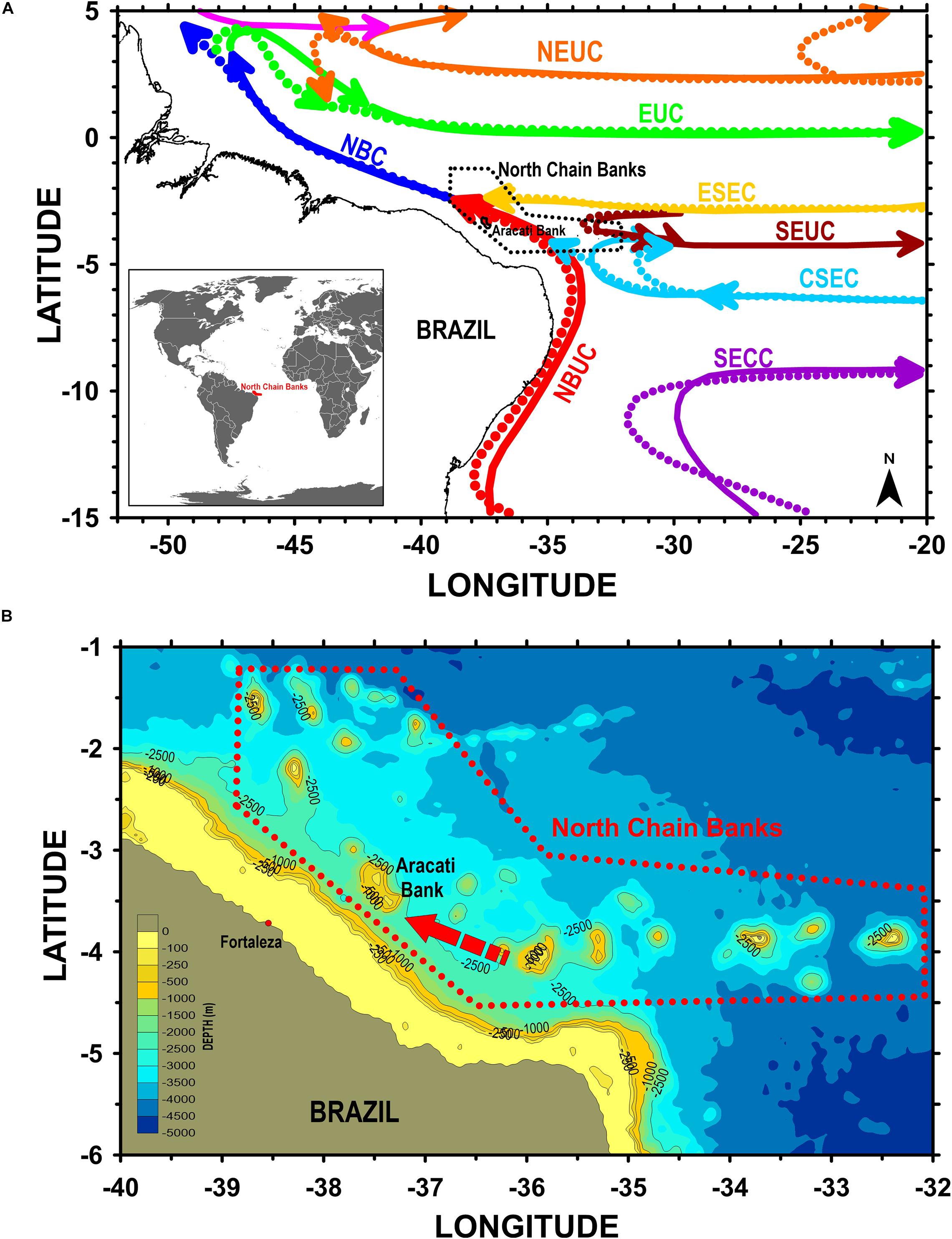
Figure 1. Study area (A) general location view of the North Chain Banks and major currents at the top 100 m (solid lines) and at 100- to 500-m layers (dashed lines), both compiled from Stramma and England (1999). (B) Detailed view of the North Chain Banks with bathymetric contours and direction of prevailing winds (dashed arrow). NEUC, North Equatorial Undercurrent; NBC, North Brazil Current; EUC, Equatorial Undercurrent; ESEC, Equatorial South Equatorial Current; SEUC, South Equatorial Undercurrent; CSEC, Central South Equatorial Current; NBUC, North Brazil Undercurrent; SECC, South Equatorial Countercurrent.

The major current system in the western tropical Atlantic in the top 100-m layer and the 100–500-m layer is presented in Figure 1A. The currents present in the NBCh domain are the North Brazil Current (NBC), the North Brazil Undercurrent (NBUC), the Central South Equatorial Current (CSEC), the Equatorial South Equatorial Current (ESEC), and the South Equatorial Undercurrent (SEUC) (Richardson and McKee, 1984; Peterson and Stramma, 1991; Stramma and England, 1999).

The NBUC and NBC follow the Brazilian coast and are characterized by a strong northwest acceleration inshore (Richardson and Walsh, 1986; Krelling et al., 2020).

The NBC is present all year. The vertical structure of the NBC between 5° and 10° S is characterized by the existence of an undercurrent with an average intensity of 80 cm.s^–1 in its nucleus, lying at a depth of approximately 200 m (Schott and Böning, 1991; Silveira et al., 1994; Schott et al., 1995, 2002). More recent modeling and observational results show the NBC core with maximum values higher than 1 m.s^–1 (Stramma et al., 2005; Krelling et al., 2020).

The existence of this structure can be explained because Ekman transport in the western tropical region opposes geostrophic flow, resulting in a typical upwelling situation. Schott et al. (1998) estimated the annual cycle of NBC transport in the oceanic layer between 0- and 500-m depth at coordinates 44° W (0°–5° N) based on the monthly measurement averages from moorings. The NBC transport value was 27.5 Sv, and the transport speed was 0.54 m.s^–1 in summer and 0.75 m.s^–1 in winter.

In the NBCh area, the southeast trade wind predominates (Figure 1B), which is the main element of the anticyclonic circulation of the South Atlantic Ocean. These winds can be observed between 35° S up to the equator during the summer (February) and between 30° S up to 10° N during winter (August); these winds are dominant throughout the year in the NBCh area.

The Aracati Bank is the larger bank in the NBCh. This bank is 56 km long and 33 km wide and is located in the area where the North Brazilian Current is strongest, exhibiting velocities of 30–50 cm.s^–1 during the summer and up to 1 m.s^–1 in August (Richardson and McKee, 1984).

Methods and Simulations

The research method involved the analysis of meteorological and physical oceanographic data gathered under the REVIZEE-NE Program around the Aracati oceanic bank and the performance of simulations with the 3D Princeton Ocean Model (POM).

Dataset

This study was performed using a subset of data gathered under the Project REVIZEE (Living Resources in the Exclusive Economic Zone). This project was a major national sampling joint effort by the Brazilian oceanographic community and Navy, performed between 1995 and 2000. Expeditions were carried out onboard NOc Antares of the Directorate of Hydrography and Navigation (DHN) of the Brazilian Navy to guarantee country sovereignty over a 200-nautical-mile band as an Exclusive Economic Zone. The efforts along the NE-Brazilian coast section comprised four oceanographic expeditions (REVIZEE NE-I, NE-II, NE-III, and NE-IV) corresponding to austral winter, summer, autumn, and spring seasons, respectively. Although a number of years have passed, this dataset remains the most complete and robust dataset available for the study area.

More recent data for the NBCh Bank area also used here correspond to conductivity, temperature, depth (CTD) profiles gathered around the eastern NBCh Banks during the ABRAÇOS II Program and at the Aracati Bank during the CAMADAS FINAS Program in 2017 and 2012, respectively.

The cruise periods, seasons, and number of CTD casts of those expeditions are summarized in Table 1, and the locations of the oceanographic sample stations, organized according to season, are shown in Figures 2A–F.

TABLE 1

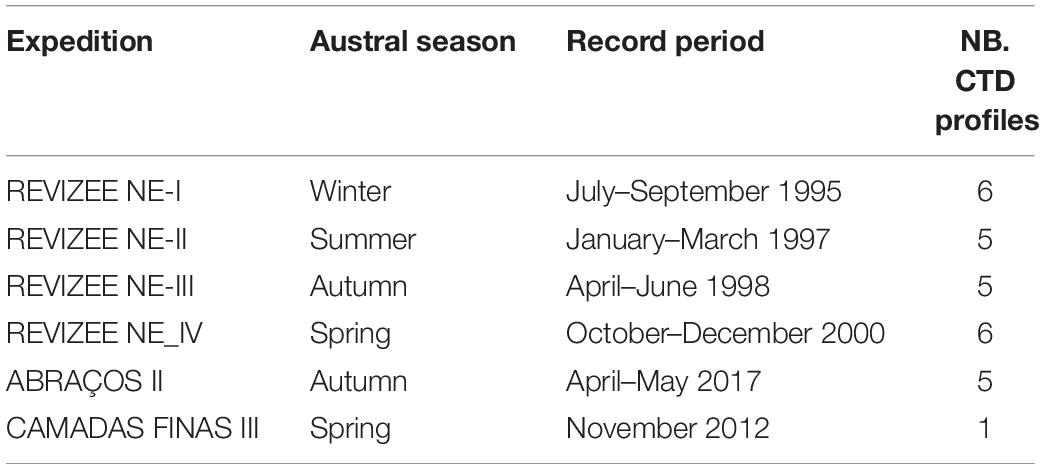
Table 1. REVIZEE-NE expeditions organized according to the seasons of the year.

FIGURE 2

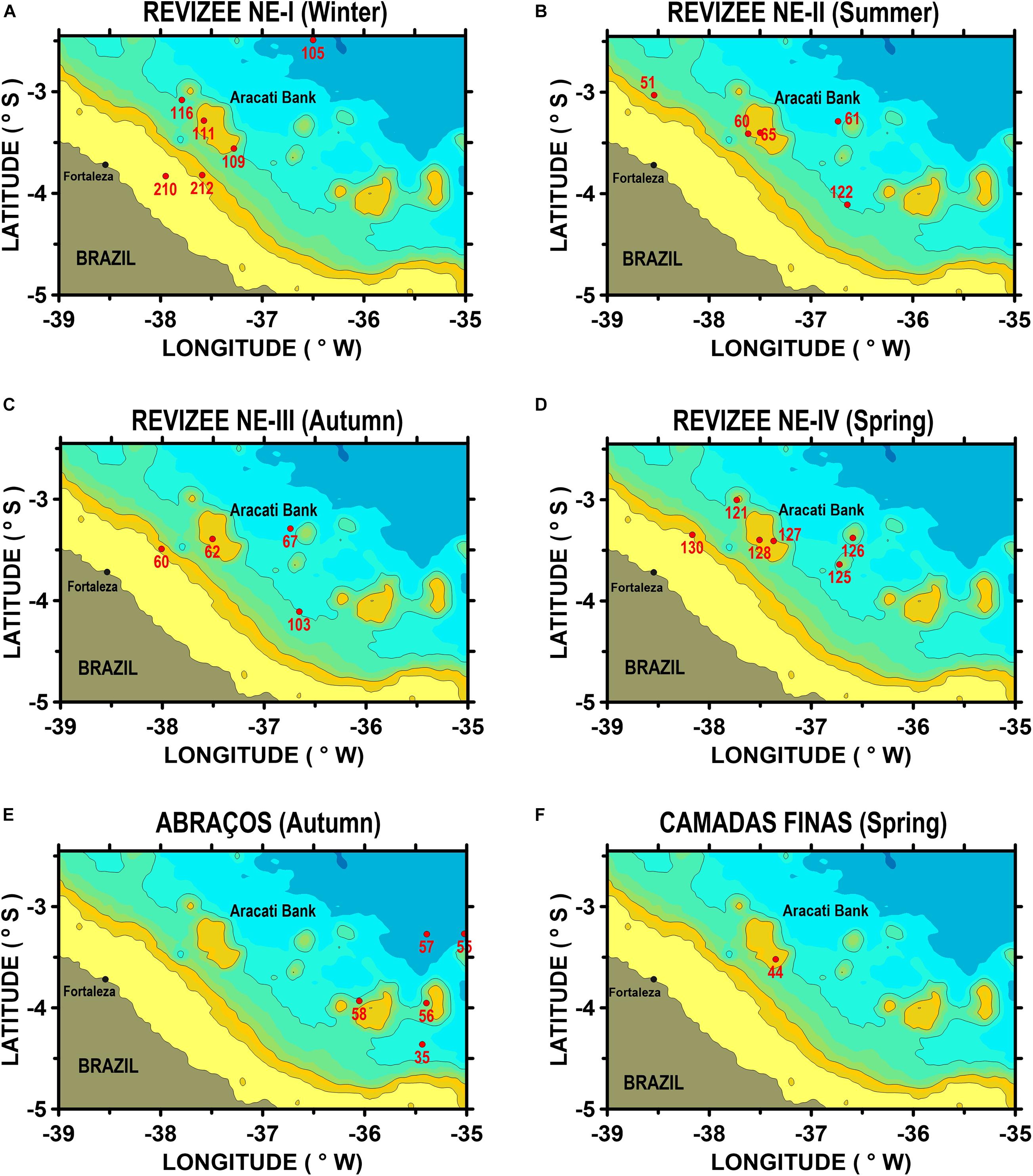
Figure 2. Study area with sampling station locations in the North Brazilian Chain (NBCh) during cruises (A) REVIZEE NE-I, winter; (B) REVIZEE NE-II, summer; (C) REVIZEE NE-III, autumn; (D) REVIZEE NE-IV, spring; (E) ABRAÇOS II, autumn; and (F) CAMADAS FINAS III, spring.

We used the data for the sampling stations corresponding to longitudinal and latitudinal transects over the Aracati Bank to investigate the effects caused by the NBC as it encounters this oceanic bank (Figures 2A–D).

At each station, wind direction and intensity were recorded using an anemometer, and the wave height and period readings were visually estimated from synoptic satellite data.

The thermodynamic dataset for this work comprised CTD continuous profiles taken with a Sea Bird Electronics SBE 911plus CTD with conductivity (resolution = 0.00004 S.m^–1), temperature (resolution = 0.0003°C), and pressure (resolution = 0.068 m) sensors and a centrifugal pump. CTD operated connected to an SBE 11plus deck unit, allowing real-time control of the data. We use a fall rate of 1 m.s^–1 and a sampling rate of 24 Hz. The maximum sampling depth around the Aracati Bank area was 800 m, which was 90% of the local depth, where areas were shallower than 800 m.

Conductivity, temperature, depth archives were transferred to a microcomputer and filtered, reduced, and edited (e.g., removing data out of water and faulty data) in preparation for analysis. Only the readings obtained during the descent of the CTD were considered. The recorded values were integrated at 5-m intervals with the first break, referred to as the surface. The calculations of the physical properties were performed in accordance with TEOS-10 (IOC et al., 2010).

T-S diagrams were then derived for the selected CTD data profiles to allow the identification of water masses present in the area, following the criteria of Barnier et al. (2001), who studied the water masses in the NBC retroflection region as described in Table 2.

TABLE 2

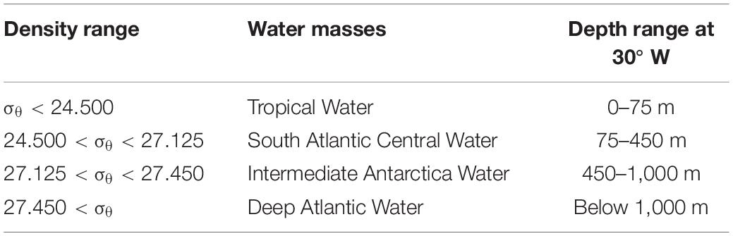
Table 2. Density range and depth limits of the water mass in the region of the Aracati Bank (Barnier et al., 2001).

Water Masses and Thermohaline Structure

The stability of the upper surface layer is an important factor that may inhibit (or facilitate) the enrichment of superficial waters. An interesting situation occurs when there are differences between the halocline and thermocline depth. If the isohaline layer is shallower than the isothermal layer, one may observe the formation of a barrier layer (BL). The barrier layer, that is, the layer between the halocline and thermocline (Lukas and Lindstrom, 1991), may isolate the upper isohaline layer from cold nutrient-rich thermocline waters, which also affects the ocean heat budget and ocean exchanges with the atmosphere (Pailler et al., 1999; Swenson and Hansen, 1999).

Most criteria that are used for determining isothermal and mixed layers in the ocean require the deviation of the temperature T (or density, σ_t) from its surface value to be smaller than a certain fixed value (Sprintall and Tomczak, 1990; Brainerd and Gregg, 1995). Normally assumed deviation from surface values for evaluating Z_T varies from 0.5°C (Wyrtki, 1964; Monterrey and Levitus, 1997) to 0.8°C (Kara et al., 2000). Z_M is estimated as the depth where density is equal to the sea surface value plus an increment Δσ_t equivalent to a desired net decrease in temperature. Miller (1976) and Spall (1991), e.g., use Δσ_t = 0.125σ_t(0) for determining the mixed layer depth, while Sprintall and Tomczak (1992) and Ohlmann et al. (1996) adopt Δσ_t = 0.5^oC(∂⁡σ_t/∂⁡T), where ∂⁡σ_t/∂⁡T is the coefficient of thermal expansion.

Following Sprintall and Tomczak (1992), we evaluate isothermal and mixed layer depths (Z_T and Z_M) in terms of temperature and density steps (ΔT and Δσ_t) from the sea surface temperature and density [T(0) and σ_t(0)]:

$$Z_T=z(T=T\left(0\right)-\mathrm{\Delta }T)(1)$$

$$Z_M=z({\mathrm{\sigma }}_t={\mathrm{\sigma }}_t\left(0\right)+\frac{\partial {\mathrm{\sigma }}_t}{\partial T}\mathrm{\Delta }T)(2)$$

where ∂⁡σ_t/∂⁡T is calculated as a function of the surface temperature and salinity (Blank, 1999). The SBE 911plus CTD has two thermometers, whose accuracy is approximately 0.001°C. Thus, for a ΔT = 0.5^oC, the error in computing Z_T is approximately 0.2% of local Z_T. The barrier layer thickness (BLT) may be easily calculated as:

$$BLT=Z_M-Z_T(3)$$

When density stratification is exclusively controlled by temperature, the isothermal layer depth becomes equivalent to the mixed layer depth and BLT=0. A particular situation occurs when the near-surface distribution of salinity is sufficiently strong to induce a pycnocline inside of the isothermal layer, or |Z_M| < |Z_T|. In this case, BLT > 0 and surface warm waters may be maintained isolated from cool thermocline waters.

Surface Energy Forcings

The upper mixed layer in the open ocean is characterized by an almost homogeneous configuration, showing reduced variations in temperature, salinity, and density profiles. This homogeneity is a result of several processes, including mixing induced by surface turbulent kinetic energy (TKE) production, such as wind- and current-driven shear and gravity wave breaking. Wind and waves in the Aracati Bank region are approximately 50% stronger during austral autumn–winter (March–August) periods than during spring–summer periods (September–February) (Geber, 2001). These distinct seasonal forcings may be evaluated by calculating the surface TKE input produced by wind shear and gravity wave breaking.

Surface TKE production by wind shear may be estimated from the analogy to the near-wall logarithmic region derived from the boundary layer theory (Klebanoff, 1955; Schilchting, 1979), where an overall balance between the production and dissipation of TKE is observed. This behavior is translated in the following form:

$$E_W=\frac{u_{{}^{*}}^2}{\sqrt{C\mathrm{\mu }}}(4)$$

where E_W is the wind-driven TKE (m².s^–2), Cμis the diffusivity coefficient (Cμ≅0.09, e.g., Rodi, 1972), and u_* is the water friction velocity, which can be estimated from classical drag coefficient formulations (Pond and Pickard, 1983, among others).

Zero-order surface wave parameters can be estimated from semiempirical formulations proposed by Stewart (1967) and Leibovich and Radhakrishnan (1977) as follows:

$$a\approx 0.1\frac{W^2}{g};T\approx 2\mathrm{\pi }\frac{W}{g};k\approx \frac{g}{W^2}(5)$$

where a is the wave amplitude (m), T is the wave period (s), k is the wave number (m^–1), g is the gravity acceleration (g≅9.81 m.s^–2), and W is the wind speed (m.s^–1). These formulations are supposed to improve wave data by providing the characteristics of surface equivalent monochromatic waves as a function of measured wind speed. The results obtained from these expressions showed good agreement with field human observations and satellite synoptic wave data (Rocha, 2000).

Other than wind shear energy, theoretical and experimental works (in situ and laboratory measurements) have shown that an important portion of TKE production at the air–water interface is associated with the presence of surface gravity waves (Gargett, 1989). This extra TKE source originates from the “wave break” phenomenon (Kitaïgorodskii et al., 1983) or is even caused by possible effects of rotational behavior in orbital movement (Cheung, 1985; Cavaleri and Zecchetto, 1987). This extra source of TKE can be evaluated from the equation proposed by Araujo et al. (2001). This formulation was obtained by using a fitting method of the field (Kitaïgorodskii et al., 1983; Drennan et al., 1992) and laboratory measurements (Cheung and Street, 1988; Thais and Magnaudet, 1996) involving the estimation of TKE intensities beneath wind waves, in the following form:

$$\mathrm{Ewa}=0.12{\left(\mathrm{\sigma }\mathrm{a}\right)}^2(6)$$

where Ewa is the wave-driven TKE (m².s^–2) and σ is the intrinsic wave frequency (s^–1). Eqs. (4, 6) give the total TKE produced at the ocean surface (E_T), or E_T = E_W + Ewa.

Numerical Simulation

The ocean model used was the POM. It is a three-dimensional ocean model developed by Blumberg and Mellor (1987). A modified version of the POM (Mellor, 1998) is employed to solve the primitive equations within a closed domain. This model uses curvilinear orthogonal horizontal coordinates, a horizontal numerical staggered “C” grid (Arakawa and Lamb, 1977), and employs a terrain-following σ-coordinate system in the vertical direction, making it well suited for the resolution of the bottom boundary layer.

Meshgrid Definition and Simulated Scenarios

The numerical study area includes a rectangular domain with four open boundaries with the Aracati Bank near the southeastern boundary. The bottom topography was defined using a nautical chart # 700 (Diretoria de Hidrografia e Navegação [DHN], 1974). The horizontal model grid includes 41 × 61 grid cells with a constant grid size of Δx = Δy = 2 km, and the maximum depth is H_max = 3,000 m.

The vertical grid includes 21 σ-layers exponentially distributed at the surface and bottom to obtain better results in the vertical layer due to the formation of important pressure gradients around and over the bank (Tchamabi et al., 2017).

All experimental data and the temperature and salinity profiles were associated with the bank shape from REVIZEE-NE cruises and used in the simulation conditions. Two seasons were considered for simulation: the austral winter season (March–August) and the austral summer season (September–February).

In a preliminary analysis of the thermodynamic properties in the study area, the simulation was enabled to verify that the information relative to the rainy season (austral autumn and winter) could be grouped into a single scenario, denoted as winter. In the same way, it was possible to group the data of the austral spring and summer periods for the numerical representation of the dry scenario, denoted as summer.

Boundary Conditions

The boundary conditions used were capable of representing the two chosen seasons. At NE and SW boundaries, symmetry conditions of von Neumann were applied. The SE boundary was laterally forced by the North Brazilian Current radiation combined with sponge layer conditions, and on the surface, the model was forced with averages of wind and heat for the grid area for both seasons from the Copernicus: Global Ocean Physics Reanalysis System Product (GLOBAL-REANALYSIS-PHY-001-030). A summary of the boundary conditions is given in Table 3.

TABLE 3

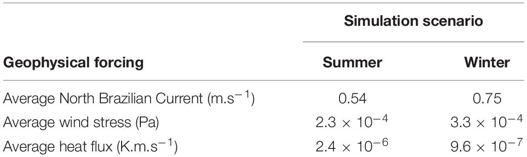
Table 3. Boundary conditions considered in simulations according to the seasons of the year.

Results and Discussion

Water Masses and Thermohaline Structure

The analysis and treatment of in situ data allowed the identification of two main water masses in the Aracati Bank area (Table 4).

TABLE 4

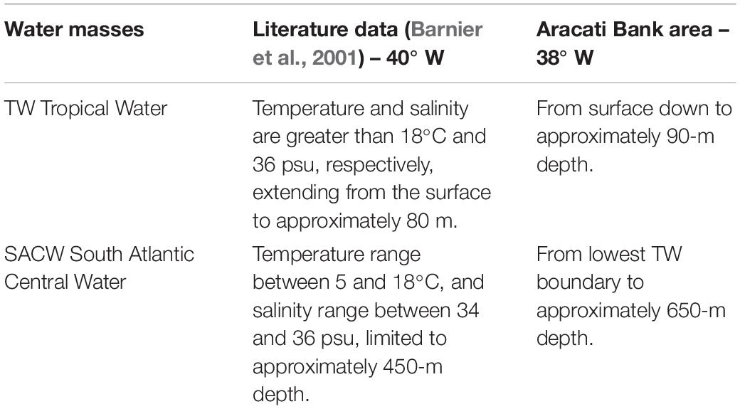
Table 4. Characteristics of the water masses identified in the Aracati Bank area.

Figures 3A–F presents the T/S diagram obtained from the field CTD profiles. The red ellipses in Figures 3A,C indicate major dispersion of the thermodynamic data near the interface between the Tropical Water and the South Atlantic Central Water masses (TW–SACW). These dispersed cloud points correspond to oceanographic data obtained from the sample stations located in the upstream region of the Aracati Bank (Geber, 2001), suggesting that it may be associated with the “deformations” in the TW–SACW interface.

FIGURE 3

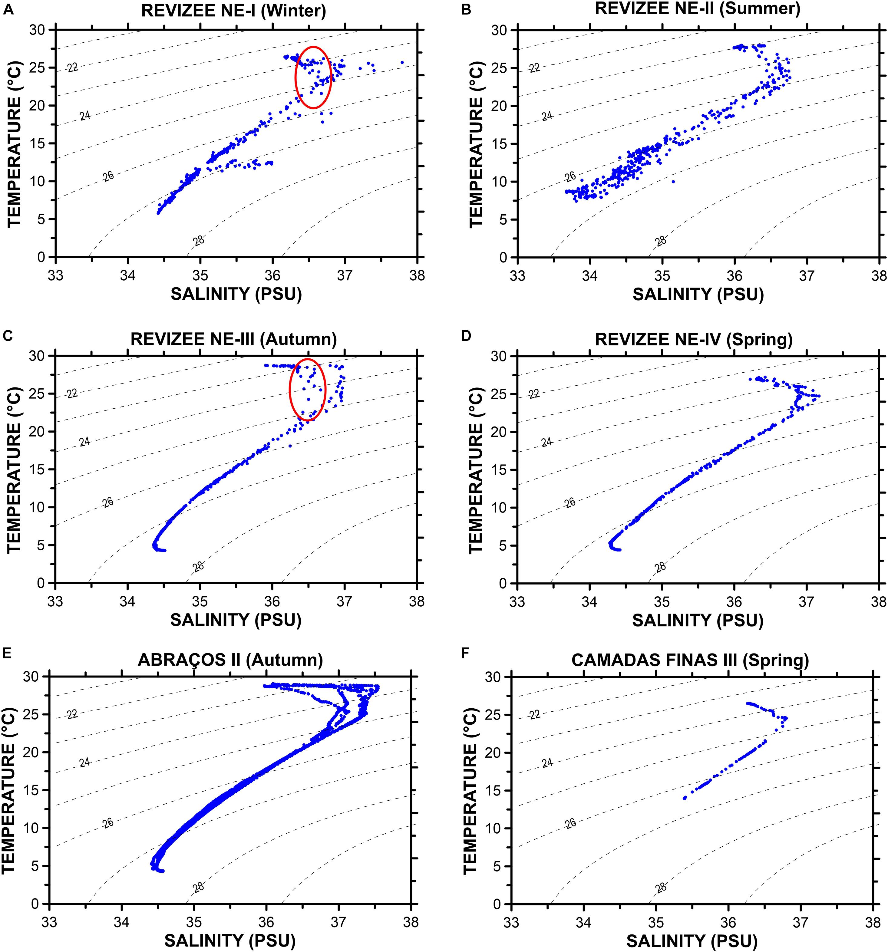
Figure 3. Seasonal variability in T/S diagrams in the Aracati Bank area during cruises (A) REVIZEE NE-I, winter; (B) REVIZEE NE-II, summer; (C) REVIZEENE-III, autumn; (D) REVIZEE NE-IV, spring; (E) ABRA OS II, autumn; and (F) CAMADAS FINAS III, spring. Blue dots are T and S field CTD data for upstream region of the Aracati Bank (Geber, 2001). The red ellipses indicate the dispersion of the termodynamical characteristics of the waters near the interface between the Tropical Water and the South Atlantic Central Water masses (TW-SACW).

Eqs. (1–3) are used in this work to evaluate the seasonal variability of the isothermal (Z_T), mixed (Z_M), and BLTs in the study area. Figure 4 presents the seasonally averaged values calculated from the CTD profiles. The results indicate higher values of Z_T, Z_M, and BLT during autumn and winter and the presence of considerably shallower layers during summer and (mainly) austral spring. The mixed layer (Z_M) depth, for example, ranged from 6 m (spring) to 84 m (winter). Following the same tendency, the isothermal layer (Z_T) was limited to 8 m during spring and reached a most important value of 96 m during winter. The resulting BLT values indicated the presence of significant BL during autumn (20 m thick), contributing to isolating surface warmer waters from deeper and colder nutrient-rich waters. Otherwise, negligible values of BLT are found during summer and (mainly) spring seasons. These periods of the year are characterized by the action of less intense winds and lower precipitation rates, while stronger surface forcings (wind and waves) observed during autumn and winter contribute to sinking the isothermal and mixed layers in the Aracati Bank area.

FIGURE 4

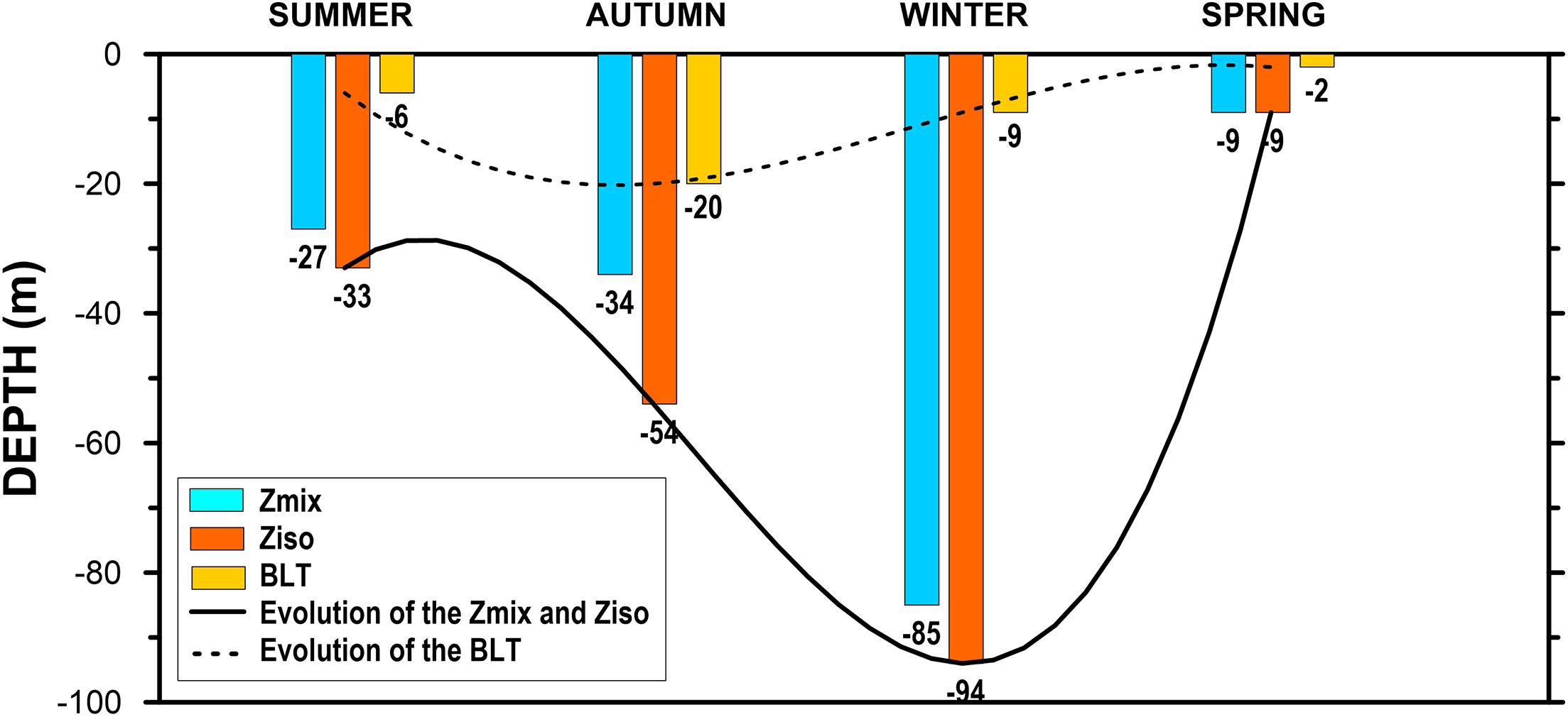
Figure 4. Seasonal variation of the average isothermal, mixed, and barrier layer thickness in the Aracati Bank area.

Surface Energy Forcings

The TKE induced by wind shear and wave breaking processes in the Aracati Bank region are calculated from Eqs. (4) to (6), respectively. These expressions result in wind-induced E_W values ranging between 3.5 × 10^–4 m².s^–2 (summer) and 2.3 × 10^–3 m².s^–2 (winter) and wave-induced E_WA values ranging from 4.6 × 10^–2 m².s^–2 (summer) to 2.1 × 10^–1 m².s^–2 (winter). This yields $\frac{E_W}{E_{WA}}=o\left(1\right)$, which is in agreement with field (Kitaïgorodskii et al., 1983; Drennan et al., 1992) and laboratory (Cheung and Street, 1988; Thais and Magnaudet, 1996) measurements obtained beneath energetically wavy surfaces. This result suggests that gravity waves are the prime candidate for driving the erosion/deepening of seasonal pycnoclines in the study area.

If one chooses wind shear energy (E_W) and wave number (k) as normalization scales, it is possible to establish a linear ratio between the total TKE (E_T = E_W + EWA) and its capacity for mixing the upper surface layers (Z_M). This relationship is represented in Figure 5. It was determined using the least-squares curve fitting method for wind speeds between 6.2 and 13.4 m.s^–1 (87% of overall field data) as follows:

FIGURE 5

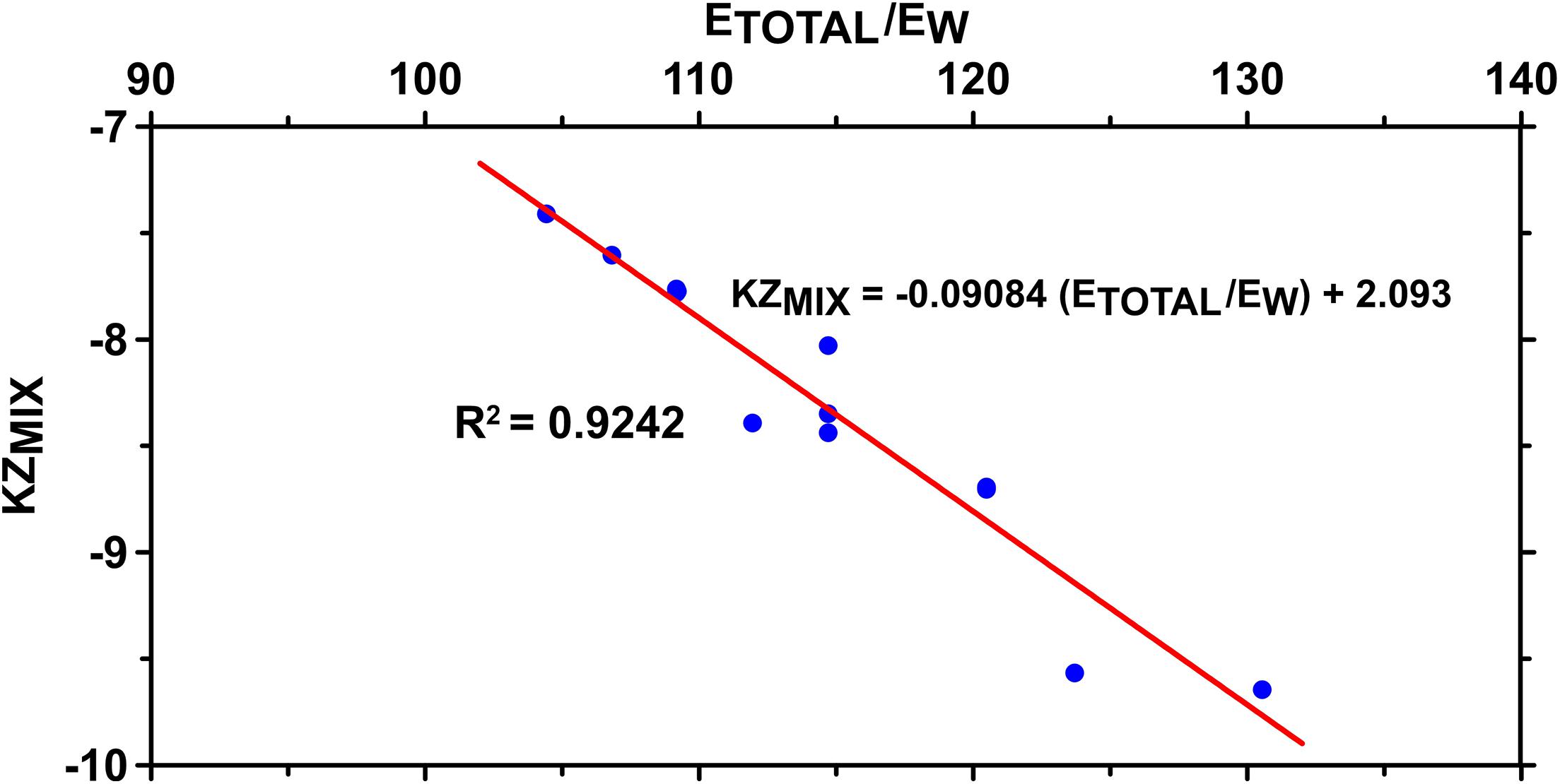
Figure 5. Values of surface energy and mixing layer depth in the Aracati Bank area (blue dots) and adjusted linear regression (red line). Linear ratio between the total TKE (ET = EW + EWA) and its capacity for mixing the upper surface layers (ZM).

$$k{Z}_M=-0.09084\frac{E_T}{E_W}+2.093\mathit{\hspace{1em}\hspace{1em}\hspace{1em}\hspace{0.5em}}\text{or}$$

$${\widehat{Z}}_M=-0.09084{\widehat{E}}_T+2.093(7)$$

where small hats represent non-dimensional variables.

A simple scale analysis involving energy and wind/wave parameters may also be performed to show that the mixing layer depth is proportional to the wave height in the following form:

$${\mathrm{E}}_{\mathrm{T}}={\mathrm{E}}_{\mathrm{W}}+\mathrm{Ewa}\equiv \mathrm{Ewa}=\mathrm{O}\left({\mathrm{\sigma }}^2{\mathrm{a}}^2\right)(8)$$

$$\mathrm{k}{\mathrm{Z}}_{\mathrm{M}}=\mathrm{O}\left(\frac{{\mathrm{\sigma }}^2{\mathrm{a}}^2}{{\mathrm{u}}_{*}^2}\right)\mathit{\hspace{1em}\hspace{0.25em}}\therefore \mathit{\hspace{1em}\hspace{0.25em}}{\mathrm{Z}}_{\mathrm{M}}=\mathrm{O}\left(\mathrm{a}\right)=\mathrm{O}\left({\mathrm{W}}^2\right)(9)$$

Expression (9) also states that the upper mixed layer depth is proportional to the square of the wind speed. Wind speeds registered during autumn–winter in the Aracati Bank region are approximately 50% higher than the measured values for spring–summer periods (Geber, 2001). These differences may then explain the seasonal evolution of mixed layer depths previously stressed from field data (Figure 4).

Model “Spin-Up” and Comparison With T/S Field Data

During the adjustment process in POM, the time step for numerical stability in the winter for the 15th day was an average global energy of 9.7 × 10³ J, and in the summer simulation, the energy stabilized for the 10th day with an average of 7.8 × 10³ J. The energy in the summer was lower, as well as the time step needed for model “spin-up.” For both winter and summer scenarios, only numerical results corresponding to the numerical time 21st day were considered, despite the fact that the model stability was being achieved before this delay.

The numerical T/S profiles were systematically compared with experimental data. Figure 6 gives some typical examples of the parallel between temperature and salinity profiles issued from numerical simulations and T/S distributions obtained from a field CTD device. The comparison of T/S profiles shows that the model is able to generate profiles correctly, even the maximum salinity at the surface that was observed in the field. This result also suggests that the model supplies good descriptions of the thermohaline structure observed from field measurements.

FIGURE 6

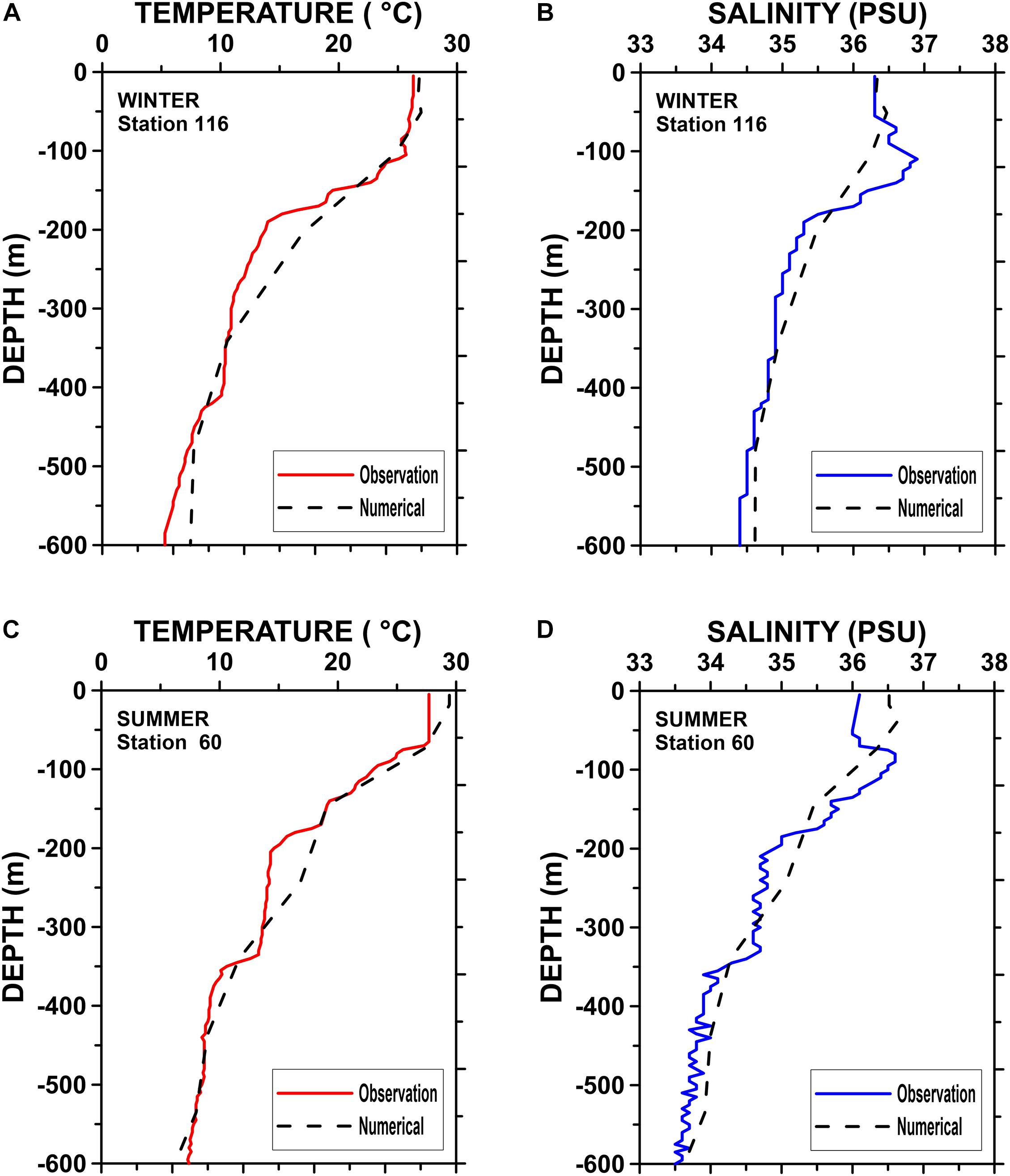
Figure 6. Comparison between experimental data and numerical simulation results for temperature and salinity profiles in the winter (A,B) and summer (C,D) seasons.

Horizontal Cinematic Structure

To analyze the horizontal circulation in the area of Aracati Bank, horizontal velocity fields were traced at depths of 50, 100, 250, 500, and 1,000 m. Figures 7A–J show the numerical velocity fields generated by the model for the winter and summer seasons.

FIGURE 7

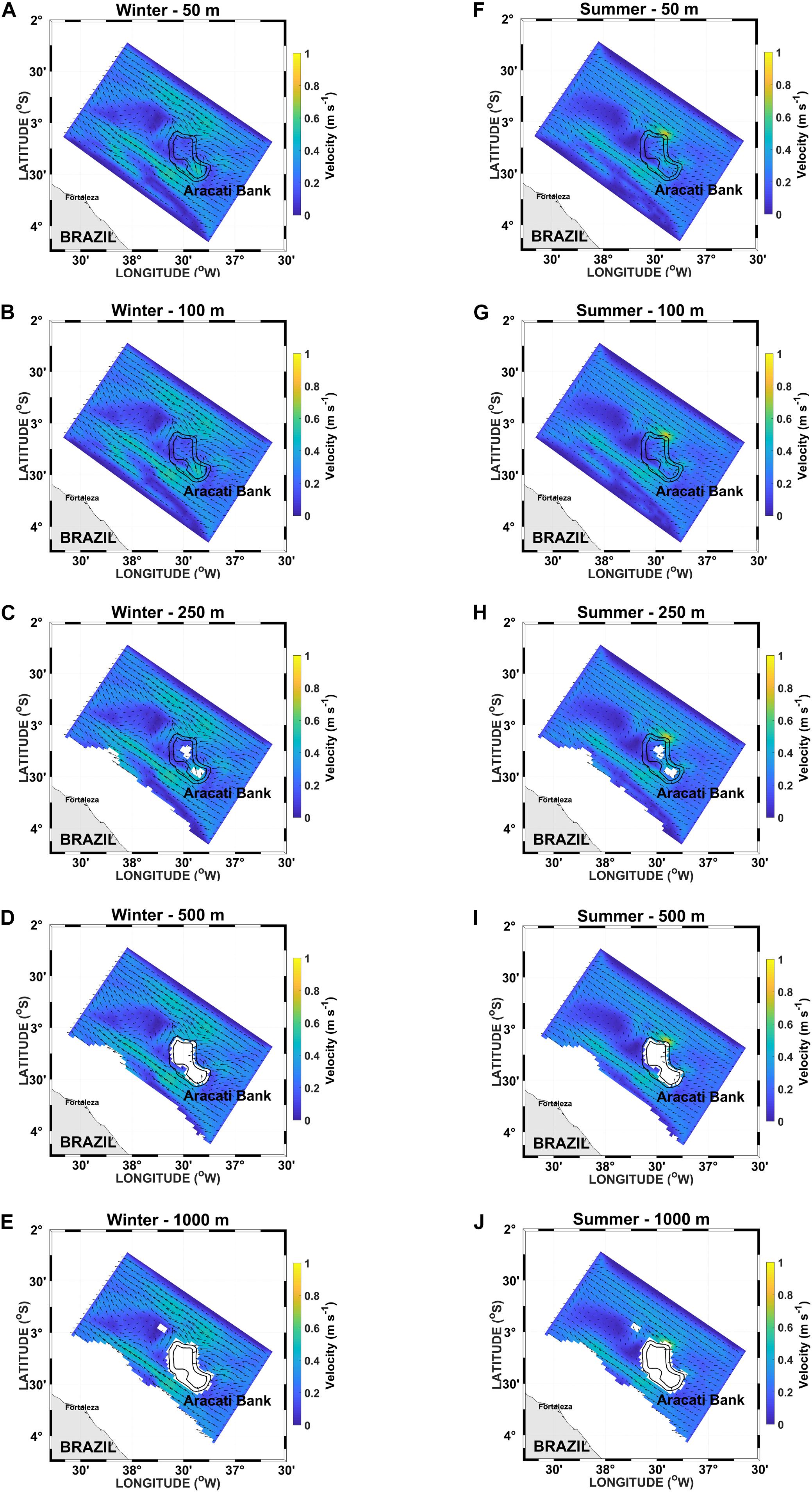
Figure 7. Horizontal velocity (m.s^{– 1}) fields in the Aracati Bank area at depths of 50, 100, 250, 500, and 1,000 m during winter (A–E) and summer (F–J) seasons.

Figures 7A–J show that the velocity vectors turn around the bank, producing eddies in the bank vicinity, especially in the upstream area, where the horizontal velocity gradients between the bank and the frontal slope are stronger.

However, in the summer season (Figures 7F–J), changes in current vector directions in the upstream bank area are less pronounced relative to winter simulations (Figures 7A–E).

Eddies made by horizontal velocities could “arrest” nutrients, plankton, and larvae that are important for increasing marine productivity. To analyze the Aracati Bank potential in producing eddies in its vicinity, the vertical component of the vorticity in the bank area was calculated as follows:

$$\stackrel{\rightharpoonup }{\mathrm{\Omega }}=\frac{\partial \overrightarrow{V}}{\partial x}-\frac{\partial \stackrel{\rightharpoonup }{U}}{\partial y}(10)$$

where $\overrightarrow{\mathrm{\Omega }}$ is the relative vertical vorticity (s^–1).

Figures 8A–J present the vertical vorticity field calculated from the horizontal velocity vectors $\overrightarrow{U}$ and $\overrightarrow{V}$. The negative results indicate clockwise vorticity, while positive results indicate counterclockwise vorticity. Figures 8A–E show that the Aracati Bank has higher potential to generate positive vorticity at depths of 50, 100, and 250 m than deeper depths. Figures 8A,B,F,G show positive vorticity values for the winter and summer seasons, indicating the potential to reduce isothermal and mixed layer depths over the bank. A comparison between the velocity fields for both the winter and summer seasons indicates that the rotational field is very similar at depths shallower than 250 m. However, at a depth of 500 m, the negative vorticity found during the winter season (Figure 8D) was not generated with the same intensity during the summer season (Figure 8I).

FIGURE 8

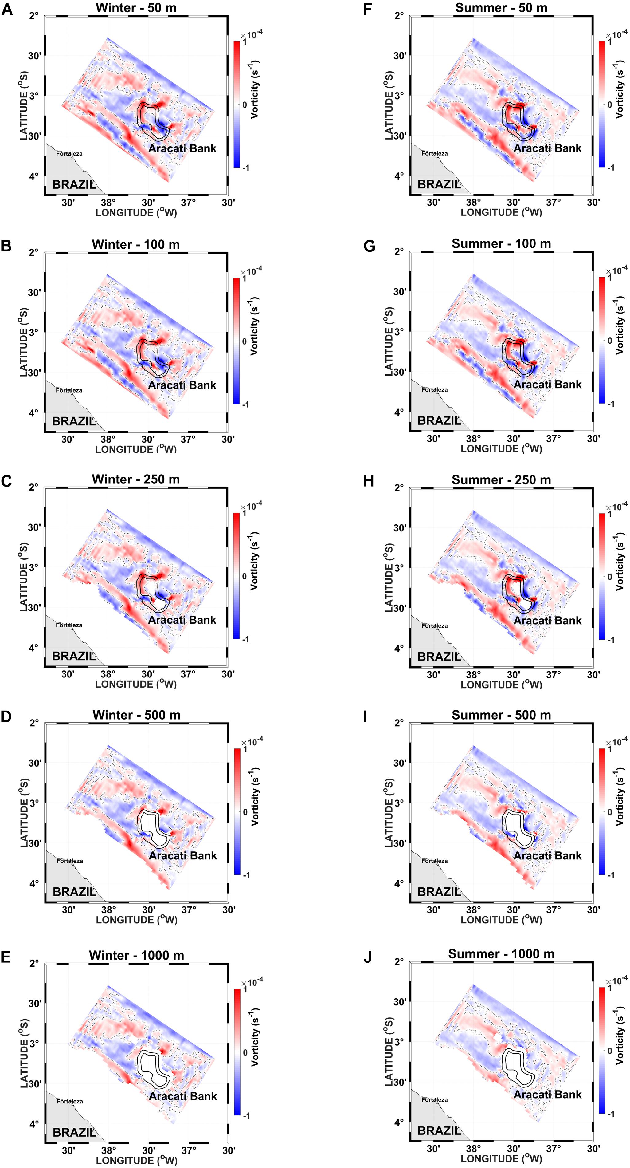
Figure 8. Vertical vorticity (s^{– 1}) in the Aracati Bank area at depths of 50, 100, 250, 500, and 1,000 m during winter (A–E) and summer (F–J) seasons.

Vertical Temperature and Velocity Structure

Figure 9 presents the temperature and vertical velocity (w) profiles obtained from simulations for both winter (Figure 9A) and summer (Figure 9B) seasons across the Aracati Bank section along the NBC. In these panels, the NBC crosses the bank from right to left.

FIGURE 9

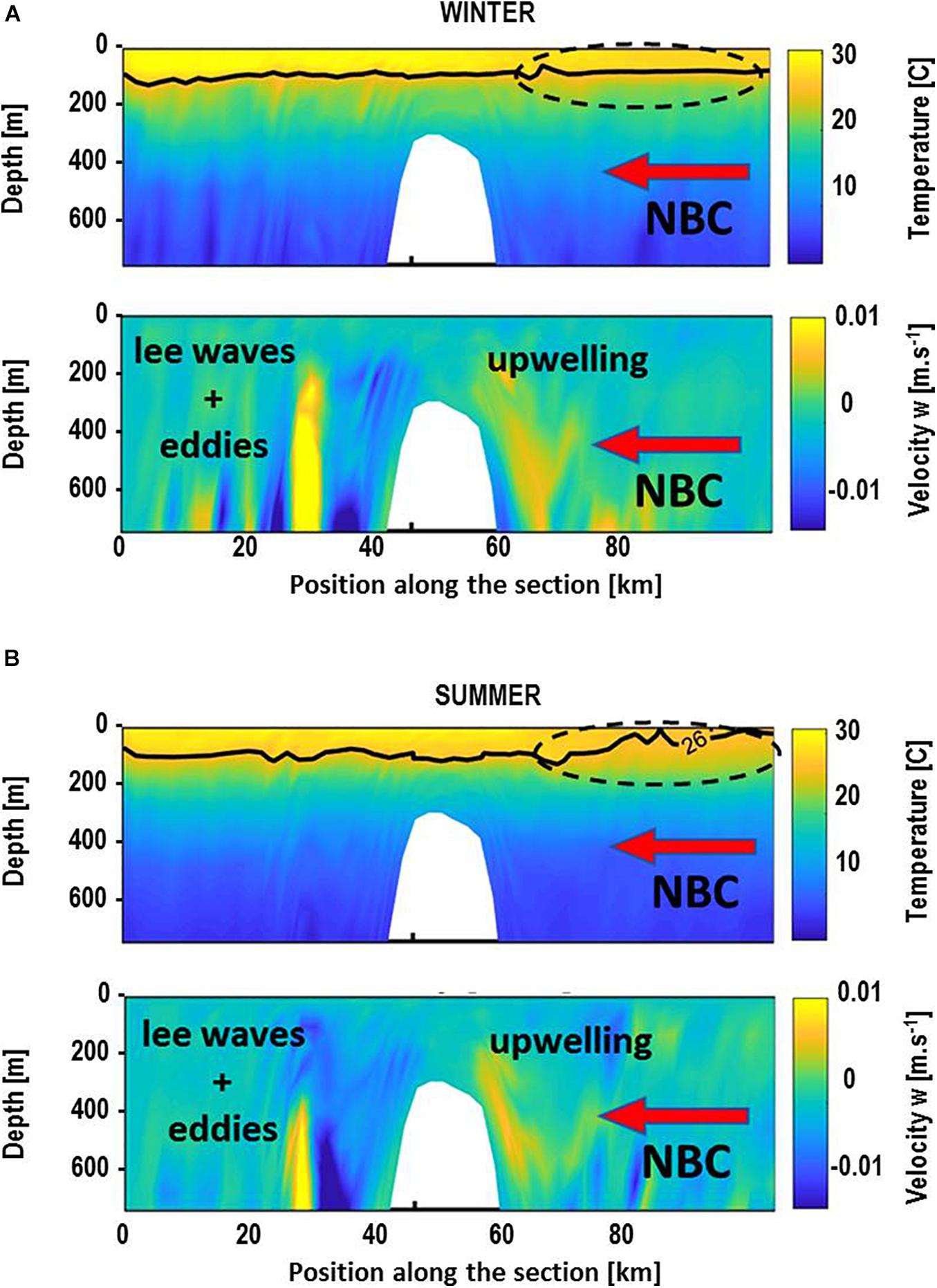
Figure 9. Temperature and w vertical velocity along a section crossing the Aracati Bank area during winter (A) and summer (B) seasons. North Brazil Current (NBC) crosses the bank from the right to the left side.

As a result of the flow-topography interaction, upstream isotherm perturbation and upwelling and downstream leeward and eddy generation were verified during both seasons.

The highest intensities in vertical velocity (Figures 9A,B) are located in the upstream bank region and tend to decrease toward the surface. The minor vertical velocity during the winter was 0.003 × 10^–3 m.s^–1 near the surface, and the major value was 8.4 × 10^–3 m.s^–1 at a 370 depth, with an average velocity of 2.2 × 10^–3 m.s^–1.

In the summer situation, these values were 0.0004 × 10^–3 m.s^–1 (near the surface) and 7.8 × 10^–3 m.s^–1 at a 266-m depth, with an average of 2.6 × 10^–3 m.s^–1. Despite being less intense, these shallower maximum vertical currents result in a more pronounced near-surface isothermal perturbation.

All values are in global agreement with different field/geophysical and theoretical studies found in the literature. For example, Chen and Beardsley (1995) performed a numerical study of stratified tidal rectification over symmetric banks and observed the presence of vorticity in the upstream bank region promoting upwelling to the surface along the bottom slope with a maximum vertical velocity of approximately 5.0 × 10^–3 m.s^–1 at 56-m depth and 1.8 × 10^–3 m.s^–1 at 83-m depth during a more energetic winter situation; while in the summer season, the vertical velocity was 1.0 × 10^–3 m.s^–1 at 120-m depth. Franks and Cheng (1996) studied the influence of physical forcing over plankton production on Georges Bank during the summer. These authors found vertical velocities of approximately 0.1 × 10^–3 m.s^–1, concluding that the phytoplankton in the well-mixed waters of the Georges Bank are nutrient replete, with an excess of nutrients supplied by physical processes. In another numerical study of stratified tidal rectification over the same bank, Cheng et al. (1995) found that, in summertime, cross-bank circulations exhibit a strong asymmetry with respect to the two sides of the bank. In this case, they observed that when the side of the bank was much steeper, the water became shallower, and the vertical mixing increased by approximately 0.1 × 10^–3 m.s^–1 at a depth of 120 m.

Conclusion

The temperature CTD profiles indicated the presence of a permanent thermocline throughout the year, located between 70- and 150-m depth. The pattern of isohaline distribution followed that of isotherm variation. At times, the formation of low-salinity eddies was verified on the Aracati Bank slope. The 3D model used was able to accurately reproduce the thermohaline structure in the Aracati Bank area. The kinematic structure observed in the performed simulations indicated vertical velocities of 10^–3 m.s^–1 in the upstream region of the bank during winter and summer seasons. During the austral summer, the most important vertical velocities were localized below the lower limit of the euphotic zone, while during the austral winter, these velocities were within the euphotic zone, favoring primary producers.

The data recorded for the Aracati Bank provided clear evidence that upwelling and consequent enrichment of the surface layer can result from a flow-topography interaction in this area, especially during the winter season. Similar uplift of isotherms was observed in October 1990 during fishing surveys near the Aracati, Guará, and Sírius seamounts (Hazin et al., 1990), reinforcing the notion that this process could occur in fairly regular basis and that they are linked in some way to the Aracati Bank topography and NBC interaction. The strong physical forcing by the NBC and southeast trade winds over the Aracati Bank contributes significantly to possible rises in thermodynamic parameters in the study region.

While the results presented here provide evidence to show that the interaction between Aracati Bank and the NBC promotes vertical mixing, the observations are limited to the relatively small spatial and temporal scales examined. Further research is still required to determine the influences of the thermodynamic parameters and analysis of complementary chemical and biological variables across different spatial and temporal scales.

Data Availability Statement

The raw data supporting the conclusions of this article will be made available by the authors, without undue reservation.

Author Contributions

All authors listed have made a substantial, direct and intellectual contribution to the work, and approved it for publication.

Funding

MA and CN acknowledge the support of the Brazilian Research Network on Global Climate Change-Rede CLIMA (FINEP grants 01.13.0353-00). This work is a contribution to the Projects INCT AmbTropic–Brazilian National Institute of Science and Technology for Tropical Marine Environments (grants 565054/2010-4, 625 8936/2011, and 465634/2014-1, CNPq/FAPESB/CAPES), International Joint Laboratory TAPIOCA (IRD-UFPE-UFRPE), and to the TRIATLAS project, which has received funding from the European Union’s Horizon 2020 Research and Innovation Program under grant agreement no. 817578.

Conflict of Interest

The authors declare that the research was conducted in the absence of any commercial or financial relationships that could be construed as a potential conflict of interest.

Acknowledgments

We thank the scientific and crew members of the NOc Antares/Brazilian Navy for their efforts during the oceanographic expedition.

References

Arakawa, A., and Lamb, V. R. (1977). Computational design of the basic processes of the UCLA general circulation model. Methods Comput. Phys. 17, 174–265.

Google Scholar

Araujo, M., Dartus, D., Maurel, P. H., and Masbernat, L. (2001). Langmuir circulations and enhanced turbulence beneath wind-waves. Ocean Modell. 3, 109–126. doi: 10.1016/s1463-5003(01)00004-x

CrossRef Full Text | Google Scholar

Araujo, M., Limongi, C. M., Servain, J., Silva, M. A., Leite, F. S., Veleda, D. R. A., et al. (2011). Salinity-induced mixed and barrier layers in the Southwestern tropical Atlantic Ocean off the Northeast of Brazil. Ocean Sci. 7, 63–73. doi: 10.5194/os-7-63-2011

CrossRef Full Text | Google Scholar

Araujo, M., Noriega, C., Medeiros, C., Lefèvre, N., Ibánhez, J. S. P., Montes, M. F., et al. (2018). On the variability in the CO₂ system and water productivity in the western tropical Atlantic off North and Northeast Brazil. J. Mar. Syst. 1:1.

Google Scholar

Assunção, R. V., Silva, A. C., Roy, A., Bourlès, B., Silva, C., Ternon, J.-F., et al. (2020). 3D characterisation of the thermohaline structure in the southwestern tropical Atlantic derived from functional data analysis of in situ profiles. Prog. Oceanogr. 187:102399. doi: 10.1016/j.pocean.2020.102399

CrossRef Full Text | Google Scholar

Barnier, B., Reynaud, T., Beckmann, A., Böning, C., Molines, J. M., Barnard, S., et al. (2001). On the seasonal variability and eddies in the North Brazil Current: insights from model intercomparison experiments. Prog. Oceanogr. 48, 195–230. doi: 10.1016/s0079-6611(01)00005-2

CrossRef Full Text | Google Scholar

Blank, H. F. (1999). Using TOPEX Satellite El Niño Altimetry Data to Introduce Thermal Expansion and Heat Capacity Concepts in Chemistry Courses. Department of Chemistry thesis, Clarksville: Austin Peay State University Clarksville.

Google Scholar

Blumberg, A., and Mellor, G. L. A. (1987). “Description of a three-dimensional coastal ocean circulation model,” in Three-Dimensional Coastal Ocean Models, ed. N. Heaps (Washington, DC: American Geophysical Union).

Google Scholar

Boyer, D., Davies, P., Holland, W., Biolley, F., and Honji, H. (1987). Stratified rotating flow over and around isolated three-dimensional topography. Phil. Trans. R. Soc. London A 322:213. doi: 10.1098/rsta.1987.0049

CrossRef Full Text | Google Scholar

Brainerd, K. E., and Gregg, M. C. (1995). Surface mixed and mixing layer depths. Deep-Sea Res. I: Oceangr. Res. Papers 42, 1521–1543. doi: 10.1016/0967-0637(95)00068-h

CrossRef Full Text | Google Scholar

Cavaleri, O., and Zecchetto, S. (1987). Reynolds stress under wind waves. J. Geophys. Res. 92, 3894–3904. doi: 10.1029/jc092ic04p03894

CrossRef Full Text | Google Scholar

Chaves, T. B. C., Mafalda, J. R. P., Santos, C., Souza, C. S., Moura, G., Sampaio, J., et al. (2006). Planktonic biomass and hydrography in the Exclusive Economic Zone of Brazilian Northeast. Trop. Oceanogr. Online 34, 12–30.

Google Scholar

Chen, C., and Beardsley, R. C. (1995). A numerical study of stratified tidal rectification over finite-amplitude banks. Part I: Symmetric bank. J. Phys. Oceanogr. 25, 2090–2110.

Google Scholar

Cheng, C., Beardsley, R. C., and Limeburner, R. A. (1995). Numerical study of stratified tidal rectification over finite – amplitude banks. Part II: Georges Banks. J. Phys. Oceanogr. 25, 2111–2128. doi: 10.1175/1520-0485(1995)025<2111:ansost>2.0.co;2

CrossRef Full Text | Google Scholar

Cheung, T. K. (1985). A study of the Turbulent Layer in the Water at an Air-Water Interface. Technical Report 287, Department of Civil Engineering, Stanford University. Stanford, CA: 229.

Google Scholar

Cheung, T. K., and Street, R. L. (1988). Wave-following measurements in the water beneath an air-water interface. J. Geophys. Res. 93, 14689–14993.

Google Scholar

Clark, M. (1999). Fisheries for orange roughy (Hoplostethus atlanticus) on sea mounts in New Zealand. Oceanol. Acta 22, 596–602.

Google Scholar

Coutinho, P. N. (1996). Levantamento do Estado da Arte da Pesquisa dos Recursos Vivos Marinhos do Brasil–Oceanografia Geológica. Região Nordeste. Programa REVIZEE. Brasília: Ministério do Meio Ambiente, dos Recursos Hídricos e da Amazonia Legal (MMA), 97.

Google Scholar

Cushman-Roisin, B. (1994). Introduction to Geophysical Fluid Dynamics. Hoboken, NJ: Prentice Hall International, 320.

Google Scholar

de Boyer Montégut, C., Madec, G., Fischer, A. S., Lazar, A., and Iudicone, D. (2004). Mixed layer depth over the global ocean: an examination of profile data and a profile-based climatology. J. Geophys. Res. C Ocean 109, 1–20.

Google Scholar

Diretoria de Hidrografia e Navegação [DHN] (1974). Carta Náutica No. 700. Brazil Costa Norte – De Fortaleza Ponta dos Três Irmãos. Escala 1:316220, Diretoria de Hidrografia e Navegação – DHN, Marinha do Brasil, 2a Edn, ed. R. J. Rio de Janeiro (Brasil: Diretoria de Hidrografia e Navegação [DHN]).

Google Scholar

Drennan, K. L., Kahma, K. K., Terray, E. A., Donelan, M. A., and Kitaïgorodskii, S. A. (1992). “Observation of enhancement of kinetic energy dissipation beneath breaking wind waves,” in Breaking Waves, eds M. L. Banner and R. H. J. Grimshaw (Berlin: Springer), 95–101. doi: 10.1007/978-3-642-84847-6_6

CrossRef Full Text | Google Scholar

Eiff, O. S., and Bonneton, P. (2000). Lee-wave breaking over obstacles in stratified flow. Phys. Fluids 12:1073. doi: 10.1063/1.870362

CrossRef Full Text | Google Scholar

Flagg, C. N. (1987). “Hydrographic structure and variability,” in Georges Banks, ed. H. Backus (Cambridge, MA: The MIT Press), 108–124.

Google Scholar

Fonteneau, A. (1991). Monts sous-marinset thons dansl’atlantique tropical est. Aquatic Living Resour. 4, 13–25. doi: 10.1051/alr:1991001

CrossRef Full Text | Google Scholar

Franks, P. J. S., and Cheng, C. (1996). Plankton production in tidal fronts: a model of Georges Bank in summer. J. Mar. Res. 54, 631–651. doi: 10.1357/0022240963213718

CrossRef Full Text | Google Scholar

Fréon, P., Barrange, M., and Aristegui, J. (2009). Eastern boundary upwelling ecosystems: integrative and comparative approaches. Progr. Oceanogr. 83, 1–14. doi: 10.1016/j.pocean.2009.08.001

CrossRef Full Text | Google Scholar

Gargett, A. E. (1989). Ocean Turbulence. Ann. Ver. Fluid Mech. 21, 419–451.

Google Scholar

Geber, F. O. (2001). Dinâmica de Bancos Oceânicos da Cadeia Norte do Brasil: Caracterização Experimental e Simulação Numérica. dissertação (Mestrado) do Departamento de Oceanografia da Universidade Federal de Pernambuco, Brasil. 98.

Google Scholar

Hazin, F. H. V., Couto, A. A., Kihara, K., Otsuka, K., and Ishino, M. (1990). Distribution and abundance of pelagic sharks in the southwestern equatorial. Atl. J. Tokio Univ. Fish. 77, 51–64.

Google Scholar

Hazin, F. H. V., Zagaglia, J. R., Broadhurst, M. K., Travassos, P. E. P., and Bezerra, T. R. Q. (1998). Review of a small-scale pelagic logline fishery off Northeastern Brazil. Mar. Fisheries Rev. 60, 1–8. doi: 10.1007/s12562-019-01360-w

CrossRef Full Text | Google Scholar

Hormazábal, S., and Yuras, G. (2007). Mesoscale eddies and high chlorophyll concentrations off central Chile (29∘ S–39∘ S). Geophys. Res. Lett. 34:L12604.

Google Scholar

Huppert, H. E., and Bryan, K. (1976). Topographically generated eddies. Deep-Sea Res. 23, 655–679. doi: 10.1016/s0011-7471(76)80013-7

CrossRef Full Text | Google Scholar

IOC, SCOR, and IAPSO (2010). The International Thermodynamic Equation of Seawater – 2010: Calculation and Use of Thermodynamic Properties. Intergovernmental Oceanographic Commission, Manuals and Guides No. 56, UNESCO (English). Paris: UNESCO, 196.

Google Scholar

Kara, A. B., Rochford, P. A., and Hurlburt, H. E. (2000). Mixed layer depth variability and barrier layer formation over the north Pacific Ocean. J. Geophys. Res. 105, 16783–16801. doi: 10.1029/2000jc900071

CrossRef Full Text | Google Scholar

Kitaïgorodskii, S. A., Donelan, A. A., Lumley, J. L., and Terray, E. A. (1983). Wave-turbulence interaction in upper ocean. Part II. Statistical characteristics of wave and turbulent components of the random velocity field in the marine surface layer. J. Phys. Oceanogr. 13, 1988–1989. doi: 10.1175/1520-0485(1983)013<1988:wtiitu>2.0.co;2

CrossRef Full Text | Google Scholar

Klebanoff, P. S. (1955). Characteristics of turbulence in a boundary layer flow with zero pressure gradient. Natl. Acad. Sci. Rep. U.S.A. 1247:19.

Google Scholar

Krelling, A. P. M., Gangopadhyay, A., Silveira, I., and Vilela-Silva, F. (2020). Development of a feature-oriented regional modelling system for the North Brazil Undercurrent region (1°–11°S) and its application to a process study on the genesis of the Potiguar Eddy. J. Operational Oceanogr. 13,, 1–13. doi: 10.1080/1755876X.2020.1743049

CrossRef Full Text | Google Scholar

Lavelle, W. J., and Mohn, C. (2010). Motion, commotion, and biophysical connections at deep ocean seamounts. Oceanography 23, 90–103. doi: 10.5670/oceanog.2010.64

CrossRef Full Text | Google Scholar

Leibovich, S., and Radhakrishnan, K. (1977). On the evolution of the system of wind drift currents and Langmuir circulations in the ocean. Part II: Structure of Langmuir vortices. J. Fluid Mech. 80, 481–507. doi: 10.1017/s0022112077001803

CrossRef Full Text | Google Scholar

Leitner, A. B., Neuheimer, A. B., Jeffrey, C., and Drazen, J. C. (2020). Evidence for long-term seamount-induced chlorophyll enhancements. Sci. Rep. 10:12729.

Google Scholar

Lessa, R. P., Mafalda, J. R. P., Advincula, R. B., Lucchesi, R. B., Bezerra, J. L. Jr., and Vaske, T. Jr., et al (1999). Distribution and abundance od icchthyoneuston at Seamounts and Island off nrth-eastern Brazil. Arch. Fish. Mar. Res. 47, 239–252.

Google Scholar

Lukas, R., and Lindstrom, E. (1991). The mixed layer of the western equatorial pacific ocean. J. Geophys. Res. 96, 3343–3357. doi: 10.1029/90jc01951

CrossRef Full Text | Google Scholar

Macedo, S. J., Montes, M. J. F., Lins, I. C., and Costa, K. M. P. (1998). Programa de Avaliação do Potencial Sustentável dos Recursos Vivos da Zona Economica Exclusiva. SCORE/NE Relatório da Oceanografia Química. Recife: UFPE.

Google Scholar

Mellor, G. L. (1998). A User’s Guide for A Three – Dimensional, Numerical Ocean Model. New Jersey, NJ: Princeton University Report. 41. Available at: http://www.researchgate.net/publication/242777179

Google Scholar

Mendonça, A. P., Martins, A. M., Figueiredo, M. P., Bashmachnikov, I. L., Couto, A., Lafon, V. M., et al. (2010). Evaluation of ocean color and sea surface temperature sensors algorithms using in situ data: a case study of temporal and spatial variability on two northeast Atlantic seamounts. J. Appl. Remote Sens. 4:043506. doi: 10.1117/1.3328872

CrossRef Full Text | Google Scholar

Miller, J. R. (1976). The salinity effect ion a mixed layer ocean model. J. Phys. Oceanogr. 6, 29–35. doi: 10.1175/1520-0485(1976)006<0029:tseiam>2.0.co;2

CrossRef Full Text | Google Scholar

Monterrey, G., and Levitus, S. (1997). Seasonal variability of mixed layer depth for the world ocean. NOAA Atlas NESDIS 14, U.S. Department of Commerce. Washington, DC: U.S. Department of Commerce, 100.

Google Scholar

Morato, T., Bulman, C., and Pitcher, T. J. (2009). Modelled effects of primary and secondary production enhancement by seamounts on local fish stocks. Deep Sea Res. Part II 56, 2713–2719. doi: 10.1016/j.dsr2.2008.12.029

CrossRef Full Text | Google Scholar

Morato, T., Varkey, D. A., Damaso, C., Machete, M., Santos, M., Prieto, R., et al. (2008). Evidence of a seamount effect on aggregating visitors. Mar. Ecol. Prog. Series 357, 23–32. doi: 10.3354/meps07269

CrossRef Full Text | Google Scholar

Mourino, B., Fernandez, E., Serret, P., Harbour, D., Sinha, B., Pingree, R., et al. (2001). Variability and seasonality of physical and biological fields at the Great Meteor Tablemount (subtropical NE Atlantic). Oceanol. Acta 24, 167–185. doi: 10.1016/s0399-1784(00)01138-5

CrossRef Full Text | Google Scholar

Ohlmann, J. C., Siegel, D. A., and Gautier, C. (1996). Ocean mixed layer depth heating and solar penetration: a global analysis. J. Clim. 9, 2265–2280. doi: 10.1175/1520-0442(1996)009<2265:omlrha>2.0.co;2

CrossRef Full Text | Google Scholar

Oliveira, A. P., Coutinhoa, T. P., Cabeçadasa, G., Brogueiraa, M. J., Cocab, J., Ramos, M., et al. (2016). Primary production enhancement in a shallow seamount (Gorringe—Northeast Atlantic). J. Mar. Syst. 164, 13–29. doi: 10.1016/j.jmarsys.2016.07.012

CrossRef Full Text | Google Scholar

Pailler, K., Bourlès, B., and Gouriou, Y. (1999). The barrier layer in the western Atlantic Ocean. Geophys. Res. Lett. 26, 2069–2072. doi: 10.1029/1999gl900492

CrossRef Full Text | Google Scholar

Peterson, R. G., and Stramma, L. (1991). Upper-level circulation in the South Atlantic Ocean. Prog. Oceanogr. 26, 1–73. doi: 10.1016/0079-6611(91)90006-8

CrossRef Full Text | Google Scholar

Pitcher, T. J., Morato, T., Hart, P. J. B., Clark, M. R., Haggan, N., and Santos, R. S. (eds) (2008). Seamounts: Ecology, Fisheries and Conservation. Fish and Aquatic Resources Series. Hoboken, NJ: Blackwell Publishing, 24.

Google Scholar

Pond, S., and Pickard, G. L. (1983). Introductory Dynamic Oceanography. Oxford: Pergamon Press, 329.

Google Scholar

Richardson, S. G. H., and McKee, T. K. (1984). Average seasonal variation of the Atlantic equatorial currents from historical ship drifts. J. Phys. Oceanogr. 17, 1226–1238. doi: 10.1175/1520-0485(1984)014<1226:asvota>2.0.co;2

CrossRef Full Text | Google Scholar

Richardson, S. G. H., and Walsh, D. (1986). Mapping climatological season variations of surface currents in the tropical Atlantic using ship drifts. J. Geophys. Res. 91, 10537–10550. doi: 10.1029/jc091ic09p10537

CrossRef Full Text | Google Scholar

Rocha, R. A. (2000). Elementos Micronutrientes na Camada Eufótica da Região Oceânica Entre Recife (PE) e Salvador (BA): Distribuição Espacial e Mecanismos Físicos Influentes na Fertilização Das Águas. Dissertação (Mestrado) do. Brasil: do Departamento de Oceanografia da Universidade Federal de Pernambuco, 129.

Google Scholar

Roden, G. I. (1991). “Effect of seamounts and seamounts chains on ocean circulation and thermohaline structure,” in Seamounts, Island and Atolls. Geophysical Monograph, Vol. 43, eds B. H. Keating, P. Fryer, R. Batiza, and G. W. Boehlert (Washington, DC: American Geophysical Union), 335–354. doi: 10.1029/gm043p0335

CrossRef Full Text | Google Scholar

Rodi, W. (1972). The Prediction of Free Turbulent Boundary Layers by Use of a Two-Equation Model of Turbulence. Ph.D. thesis. London: University of London, 310.

Google Scholar

Rogers, A. D. (1994). “The biology of seamounts,” in Advances in Marine Biology, ed. M. Lesser (London: Academic Press), 305–350. doi: 10.1016/s0065-2881(08)60065-6

CrossRef Full Text | Google Scholar

Rossi, V., López, C., Hernández-García, E., Sudre, J., Garçon, V., Morel, Y., et al. (2009). Surface mixing and biological activity in the four Eastern boundary upwelling systems. Nonlinear Process. Geophys. 16, 557–568. doi: 10.5194/npg-16-557-2009

CrossRef Full Text | Google Scholar

Rossi, V., Lopez, C., Sudre, J., Hernandez-Garcia, E., and Garçon, V. (2008). Comparative study of mixing and biological activity of the Benguela and Canary upwelling systems. Geophys. Res. Lett. 35:L11602.

Google Scholar

Schilchting, H. (1979). Boundary layer theory. New York, NJ: McGraw-Hill B. C, 489.

Google Scholar

Schott, F. A., and Böning, W. (1991). The WOCE model in the western equatorial Atlantic: upper-layer circulation. J. Geophys. Res. 96, 6993–7004. doi: 10.1029/90jc02683

CrossRef Full Text | Google Scholar

Schott, F. A., Brandt, P., Hamann, M., Fischer, J., and Stramma, L. (2002). On the boundary flow off Brazil at 5-10o S and its connection to the interior tropical Atlantic. Geophys. Res. Lett. 29, 21–21. doi: 10.1029/2002gl014786

CrossRef Full Text | Google Scholar

Schott, F. A., Fischer, J., and Stramma, L. (1998). Transports and pathsways of the upper-layer circulation in the western tropical Atlantic. J. Phys. Oceanogr. 28, 1904–1928. doi: 10.1175/1520-0485(1998)028<1904:tapotu>2.0.co;2

CrossRef Full Text | Google Scholar

Schott, F. A., Stramma, L., and Fischer, J. (1995). The warm water inflow into the western tropical Atlantic boundary regime, spring 1994. J. Geophys. Res. 100, 24745–24760. doi: 10.1029/95jc02803

CrossRef Full Text | Google Scholar

Silveira, I. C. A., Miranda, L. B., and Brown, W. S. (1994). On the origins of the North Brazil Current. J. Geophys. Res. 99, 22501–22512. doi: 10.1029/94jc01776

CrossRef Full Text | Google Scholar

Spall, M. A. (1991). A diagnostic study of wind- and buoyancy- driven north Atlantic circulation. J. Geophys. Res. 96, 18509–18518. doi: 10.1029/91jc01957

CrossRef Full Text | Google Scholar

Sprintall, J., and Tomczak, M. (1990). Salinity Considerations in the Oceanic Surface Mixed Layer. Ocean Sciences Institute Rep. 36. Sidney: University of Sidney, 170.

Google Scholar

Sprintall, J., and Tomczak, M. (1992). Evidences of the barrier layer in the surface layer of the tropics. J. Geophys. Res. 97, 7305–7316. doi: 10.1029/92jc00407

CrossRef Full Text | Google Scholar

Stewart, R. W. (1967). Mechanics of the air-sea interface. Phys. Fluids Suppl. 10, 47–55.

Google Scholar

Stramma, L., and England, M. (1999). On the water masses and mean circulation of the South Atlantic Ocean. J. Geophys. Res. 104, 20863–20883. doi: 10.1029/1999jc900139

CrossRef Full Text | Google Scholar

Stramma, L., Rhein, M., Brandt, P., Dengler, M., Böning, C., and Walter, M. (2005). Upper ocean circulation in the western tropical Atlantic in boreal fall 2000. Deep Sea Res. Part I 52, 221–240. doi: 10.1016/j.dsr.2004.07.021

CrossRef Full Text | Google Scholar

Swenson, M. S., and Hansen, D. V. (1999). Tropical Pacific Ocean mixed layer heat budget: the Pacific cold tongue. J. Phys. Oceanogr. 29, 69–81. doi: 10.1175/1520-0485(1999)029<0069:tpomlh>2.0.co;2

CrossRef Full Text | Google Scholar

Tchamabi, C. C., Araujo, M., Silva, M., and Bourlès, B. (2017). A study of the Brazilian Fernando de Noronha island and Rocas atoll wakes in the tropical Atlantic. Ocean Modell. 111, 9–18. doi: 10.1016/j.ocemod.2016.12.009

CrossRef Full Text | Google Scholar

Thais, L., and Magnaudet, J. (1996). Turbulent structure beneath surface gravity waves sheared by the wind. J. Fluid Mec. 328, 313–344. doi: 10.1017/s0022112096008749

CrossRef Full Text | Google Scholar

Travassos, P., Hazin, F. H. V., Zagaglia, J. R., Advincula, R., and Schober, J. (1999). Thermohaline structure around seamounts and islands off North-Brazil. Arch. Fishery Mar. Res. 47, 211–222.

Google Scholar

Varela, J., Araújo, M., Bove, I., Cabeza, C., Usera, G., Martí, A. C., et al. (2007). Instabilities developed in stratified flows over pronounced obstacles. Physica A : Stat. Mech. Appl. 386, 681–685. doi: 10.1016/j.physa.2007.08.051

CrossRef Full Text | Google Scholar

Watling, L., and Auster, P. J. (2017). Seamounts on the high seas should be managed as vulnerable marine ecosystems. Front. Mar. Sci. 4:14. doi: 10.3389/fmars.2017.00014

CrossRef Full Text | Google Scholar

Wessel, P., Sandwell, D. T., and Kim, S.-S. (2010). The global seamount census. Oceanography 23, 24–33. doi: 10.5670/oceanog.2010.60

CrossRef Full Text | Google Scholar

White, M., and Mohn, C. (2004). Seamounts: a review of physical processes and their influence on the seamount ecosystem. OASIS Rep. 38, 1–40. doi: 10.1002/9780470691953.ch1

CrossRef Full Text | Google Scholar

Wyrtki, K. (1964). The thermal structure of the eastern Pacific Ocean. Deutsche Hydrographische Zeitung Ergänzungsheft A 6:84.

Google Scholar

Yesson, C., Clark, M. R., Taylor, M. L., and Rogers, A. D. (2011). The global distribution of seamounts based on 30 arc seconds bathymetry data. Deep. Res. Part I 58, 442–453. doi: 10.1016/j.dsr.2011.02.004

CrossRef Full Text | Google Scholar