Assessing the Skill of a High-Resolution Marine Biophysical Model Using Geostatistical Analysis of Mesoscale Ocean Chlorophyll Variability From Field Observations and Remote Sensing

Introduction

Mesoscale variability of phytoplankton biomass and chlorophyll a, including “patchiness,” has long been observed in the global ocean, where mesoscale is defined here as O(10–100 km) and weeks-months (e.g., Mackas et al., 1985; McGillicuddy, 2016). Much debate has centered around marine phytoplankton stock variability as either being a passive reflection of the mesoscale turbulent physical flow or a response to biological rate heterogeneity arising from the resulting variable nutrient, light, stability fields, and mobile grazers (Denman and Platt, 1976; Currie and Roff, 2006). Sorting through impacts of biological, chemical, and physical interactions varying in space and time is an active area of research (McGillicuddy, 2016), and it is increasingly clear that the impacts of currents, fronts, and eddies on marine ecosystems are dynamic, evolving as a function of geography, season, and biological state. Understanding these interactions and their biogeochemical impacts ultimately informs fisheries management and also the quantification of export production and the biological pump (Harrison et al., 2018).

The complexity of biophysical variability is often difficult to resolve in observational studies, so our understanding can benefit from the use of numerical models (McGillicuddy and Franks, 2019). Within these models, realistic representations of chlorophyll a are necessary for accurate estimates of primary production. At global or even basin scales, resolving mesoscale ocean processes has been limited by computing power, and thus the physical ramifications of mesoscale eddies often have been accounted for by parameterizations of isopycnal mixing and eddy-induced transport in low-resolution simulations (Gent and Mcwilliams, 1990). These low-resolution ocean models have been used for most multi-decadal hindcasts of marine ecosystem and ocean biogeochemical dynamics, as well as almost all century-scale coupled Earth System Model projections of future climate change (e.g., Bonan and Doney, 2018). With the emergence of routine, high-resolution, global-scale simulations comes new opportunities to test the impact of parameterizations in more computationally accessible low-resolution simulations and to investigate specific science questions on mesoscale biophysical dynamics.

Before we can use the model to evaluate the origins of biological patchiness, we need to validate the model skill of not only reproducing the mean field but also of simulating the variability. The physical oceanography community has invested considerable effort in developing, comparing, and evaluating the model skill of ocean simulations across horizontal scales. Studies on paired ocean simulations from eddy-resolving (nominally 1/10th degree and smaller) through eddy-permitting to non-eddy resolving (nominally 1 degree and larger) demonstrate how mesoscale processes affect physical variability as well as the modeled ocean mean state (e.g., thermocline depth, overturning circulation, location, and strength of boundary currents; Bryan et al., 2007). Standard ocean physical metrics have been developed for assessing the magnitude and spatial and temporal patterns of simulated mesoscale variability, including comparisons against drifter and satellite-derived eddy kinetic energy, sea surface height anomalies, and sea surface temperature variability (Hurlburt et al., 2009).

Ocean biological tracers have different source and sink patterns and time-scales than physical tracers, and thus parameterizations, horizontal resolutions, and scale closures that are adequate for physics may still be insufficient for simulating ocean biology and biogeochemistry (Doney, 1999). Therefore, a similar systematic assessment of mesoscale biophysical simulations is warranted, examining both model dynamics and evaluating model skill of biological metrics relative to observational constraints from ships, autonomous platforms, and satellite remote sensing (Capotondi et al., 2019). Such efforts build on experience with biophysical model-data evaluation of simulated seasonal cycles, spatial climatologies, and interannual variability in low-resolution global and regional models (Doney et al., 2009; Stow et al., 2009) and require increasing focus on specific techniques for characterizing the behavior simulated mesoscale variability at a global scale.

Early studies on basin-scale mesoscale biophysical simulations illustrated how mesoscale features alter vertical stratification, mixed layer depths, and upwelling velocities, thus modulating nutrient and light supply for phytoplankton and biological productivity (Oschlies and Garçon, 1998; McGillicuddy et al., 2003). Recent work has continued down this thread, showing that improved representation of the mean ocean circulation at high-resolution changes the simulated biophysical interactions, altering regional primary production (Clayton et al., 2017) and bringing regional carbon export more in line with observations (Harrison et al., 2018). Harrison et al. (2018) showed that simulations without mesoscale resolution can over- or underestimate local export production by 50%, particularly in energetic regions. Mesoscale modeling simulations are also used to explore large-scale patterns and variability of properties ranging from air-sea gas fluxes to plankton community structure and biodiversity.

Because of data limitations, the possible metrics for directly evaluating simulated mesoscale biophysical dynamics is rather limited. Following previous studies (e.g., Hurlburt et al., 2009), we focus on the variability of surface ocean chlorophyll a, where there is a wealth of data from underway ship observations, moorings, autonomous platforms, and satellite remote sensing. Model mesoscale variability in surface chlorophyll a manifests as an emergent property of coupled physical-biological processes, and explicitly examining simulated chlorophyll a variability may provide insight into whether the hypotheses underlying the model’s formulation are not incorrect—and would enable studies using the model to evaluate the origins of phytoplankton patchiness.

We focus here on analyzing the skill of a high-resolution, eddy-resolving biophysical ocean simulation in capturing magnitude and length scales of observed phytoplankton variability using structure function (variogram) analysis (Journel and Huijbregts, 1978; Clark, 1987). This geostatistical technique (Cressie, 1993) has been used in the past to characterize variability in ocean surface chlorophyll a observations (Denman and Freeland, 1985; Yoder et al., 1987; Doney et al., 2003; Tortell and Long, 2009; Glover et al., 2018), and importantly, does not require gap-filling as is required for spectral analysis of chlorophyll a variability (Platt, 1972; Denman and Platt, 1976; Steele and Henderson, 1979; Gower et al., 1980; Weber et al., 1986; Denman and Abbott, 1988, 1994). Structure function analysis reveals the magnitude of spatial variability resolved in the data (sill), the spatial length scales at which the observations become independent (range), and the unresolved noise in the data (nugget).

We concentrate our analysis on the western North Atlantic Ocean where pronounced mesoscale eddies are thought to play a large role in controlling the total magnitude of the annual phytoplankton bloom, the largest spring bloom in the world (McGillicuddy et al., 2003; McGillicuddy, 2016; Behrenfeld et al., 2019). The region encompasses a range of environments, each with its own dynamical regime from the oligotrophic subtropical gyre to the Gulf Stream to the subpolar gyre (Della Penna and Gaube, 2019). This study is aided by ship and airborne observational data from field campaigns in this region carried out through the North Atlantic Aerosols and Marine Ecosystems Study [NAAMES, (Behrenfeld et al., 2019)] and prior satellite ocean color remote sensing analysis by Glover et al. (2018).

Materials and Methods

Numerical Simulation

We analyzed output from an eddy-resolving, 0.1° (∼10 km), global simulation of the ocean and sea-ice components of the Community Earth System Model (CESM; Harrison et al., 2018). The CESM ocean component used was the Parallel Ocean Program version 2 (Smith et al., 2010), and biogeochemistry was simulated with the Biogeochemical Element Cycle model (Moore et al., 2013). The model was initialized with World Ocean Circulation Experiment temperature and salinity and global climatology of biogeochemical variables [see Harrison et al. (2018) for more complete details on model parameterizations, initialization, spin-up, forcing, and integration]. Following initialization, the simulation was integrated for 5 years, with model output data saved as 5-day means. We analyzed output from years 4 and 5 of the simulation, subset for the western North Atlantic Ocean (25–55°W, 30–60°N), and used the surface total chlorophyll a concentration as the biological tracer for the geostatistical analysis.

Simulated chlorophyll a concentrations from this model have been shown to match observed mean fields reasonably well for basin-scale to global patterns (Harrison et al., 2018), but the model has not been evaluated at the regional scale. Yang et al. (2020), who compared aspects of the simulated bio-physical seasonal cycle against observations from profiling floats and satellite ocean color imagery in the NAAMES region of the western North Atlantic, pointed to potential model deficiencies, but the comparison was hindered by challenges matching data in space and time. Specifically, the high-resolution ocean model generates its own independent mesoscale turbulent field, hindering the utility of point-to-point comparisons but illustrating the value of statistical skill metric comparisons for mesoscale variability (Doney, 1999).

Observations

Ship-based observations of surface ocean chlorophyll a concentration were acquired as part of the four campaigns of NAAMES in the western North Atlantic (Behrenfeld et al., 2019). The cruises took place November 6 -December 1, 2015 (NAAMES 1), May 11 -June 5, 2016 (NAAMES 2), August 30-September 24, 2017 (NAAMES 3), and March 20-April 13, 2018 (NAAMES 4) to capture different bloom stages at different times in the seasonal cycle. Surface-water spectral absorption was measured continuously underway on the research ship using an ac-s hyperspectral absorption and attenuation meter (Sea-Bird Scientific), and particulate absorption was determined using a calibration-independent method by differencing total and dissolved absorption each hour (Slade et al., 2010). Chlorophyll a concentrations were derived using the line height method (Roesler and Barnard, 2013), where the particulate absorption in the red (676 nm) is regressed against independently-derived chlorophyll a concentration from extracted pigment samples; the relationship was calculated specifically for the NAAMES data. Data, originally collected at an average frequency of one measurement per 0.3 km, was then interpolated using a piecewise cubic interpolation onto a 9 km grid for comparison to model and satellite products. This interpolation shows no appreciable impact on the resolved variability (Supplementary Figure 1).

Satellite Ocean Color Data

Geostatistical analysis of remotely sensed surface chlorophyll a was completed in Glover et al. (2018) and those results are used for comparison here. They considered global surface chlorophyll a concentration derived from 13 years of SeaWiFS (1998–2010) to 8 years of MODIS/Aqua (2003–2010) using OC4 and OC3M algorithms (O’Reilly et al., 2000), and we have subset results from the western North Atlantic here. SeaWiFS and MODIS/Aqua level-3 imagery have a nominal resolution of 9 km. The same mathematical approach (detailed below) and programming scripts (in MATLAB^®) were used in our analysis as in Glover et al. (2018) for a consistent comparison.

Variogram Analysis

Variogram, or structure function analysis, is a geostatistical approach that provides us with an analytical expression of how the spatial variance/covariance of a field changes as a function of distance and direction, even if the sampled data has gaps as is common with satellite and field observations (Cressie, 1993; Doney et al., 2003; Glover et al., 2018). The empirical semivariance (γ^∗) in 1 dimension is given by:

${\mathrm{\gamma }}^{*}\left(\mathbf{h}\right)=\frac{1}{2N(\mathbf{h})}\sum _k^{N(\mathbf{h})}{[C^{\prime }\left({\mathbf{\text{x}}}_k\right)-C^{\prime }\left({\mathbf{\text{x}}}_k+\mathbf{\text{h}}\right)]}^2(1)$

Where h is the vector of distances between data pairs, N(h) is the number of data pairs at each distance, C’ is the data anomaly from a Reynolds decomposition involving the removal of a large-scale spatial mean field, and x_k is a spatial location in the data set (Cressie, 1993). The semivariogram is applied in 2-D using the full vector of potential data pairs.

The C’ anomaly field is assumed to contain variance from two sources, spatially-correlated variability from sub-mesoscale and mesoscale process and spatially uncorrelated noise. Generally, as data pairs get further apart they are less likely to be influenced by small-scale spatial correlations, and therefore the semi-variance is expected to increase with h. The lag distance at which that increase saturates at a plateau is the distance at which the data becomes independent, i.e., do not covary. To identify the height of that plateau (the sill) and the distance at which it occurs (the range), we fit the empirical variogram with a nonlinear regression model. Here we use a spherical model (Cressie, 1993):

$\mathrm{\gamma }\left(\mathbf{h}\right)=\{\begin{array}{c}{c}_0+\left(c_{\mathrm{\infty }}-c_0\right)\left[\frac{3}{2}\frac{\mathbf{h}}{d}-\frac{1}{2}\frac{h^3}{d^3}\right]\mathit{\hspace{1em}\hspace{0.5em}\hspace{1em}}\text{for}h\le d\hfill \\ c_{\mathrm{\infty }}\mathit{\hspace{1em}\hspace{1em}\hspace{1em}\hspace{1em}\hspace{1em}\hspace{1em}\hspace{1em}\hspace{1em}\hspace{1em}\hspace{1em}\hspace{1em}\hspace{1em} }\text{for}h>d;\hfill \end{array}(2)$

Where c_o is the unresolved variance (or nugget) from spatially uncorrelated noise and/or sub-grid scale processes, c_∞ is the total variability (the sill) at distances exceeding the correlation length scale, d is the decorrelation length scale (range). The relative sill, which represents the resolved variability, is then the difference between c_∞ and c₀. Relative sill (resolved variability) is reported as directly computed from Eq. 2 unless explicitly stated to be in terms of the coefficient of variation (CV equal to standard deviation divided by the mean) or the arithmetic standard deviation (Glover et al., 2018).

Processing and Analysis

Our analysis approach matched that of Glover et al. (2018). Before geostatistical analysis, all surface chlorophyll a estimates were log₁₀ transformed to follow past convention (e.g., Glover et al., 2018) and because, to first order, it produces roughly normal distributions for the time and space sub-domains used to compute geostatistics (Campbell, 1995). To isolate anomalies, we used a 200 km spatial low-pass filter with a 31-day Hamming window in the N-S and E-W directions to remove variability larger than mesoscale and subtract the large-scale mean. Model output was divided into 5° × 5° boxes, and fully 2-dimensional empirical variograms were computed for each 5-day time step using a Fast Fourier Transform-based variogram approach (Marcotte, 1996). A 1-D spherical model (forced with a zero nugget for the CESM model output) was then fit to monthly composites of those empirical variograms using a Levenberg-Marquardt nonlinear regression routine to find a monthly composite sill and range in the North-South and East-West directions for each grid box.

Underway field observations of chlorophyll a were interpolated onto a 9 km grid to more closely match that of the model (∼9 km) and satellite (9 km) data. At this resolution, both the resolved and unresolved variability recovered are a combination of mesoscale and submesoscale variability, with most of the latter likely being found in the nugget. The gridded field observational data were then split into linear segments to avoid zig-zags in the path, and a linear detrend was applied. We then calculated the 1-D empirical variogram and fit that using a spherical model.

Results

The western North Atlantic region of focus here spans from the upwelling-favorable subpolar gyre to the seasonally stratified subtropical oligotrophic gyre separated by a temperate zone and energetic Gulf Stream (see Della Penna and Gaube, 2019). Overall, regional surface ocean chlorophyll a concentrations in the model and in field observations peak in May with a pronounced seasonal cycle in the northern sector [Figure 1; see also Behrenfeld et al. (2019) and Yang et al. (2020)]. Surface chlorophyll a concentrations remain relatively low (<0.15 mg/L) year-round in the subtropical gyre, but the northern extent of the oligotrophic region varies over time, pushing northward in the Spring and Fall. The model produces high chlorophyll a bands near the coast in the temperate region surrounding the core of the subpolar gyre. Previous work, including a recent study by Yang et al. (2020), has shown that the model may be overestimating productivity at that frontal region. In contrast, field observations document higher chlorophyll a in May in the more central subpolar region than is seen in the model results (Figure 2). Field observations closely resemble SeaWiFS and MODIS climatology for the region.

FIGURE 1

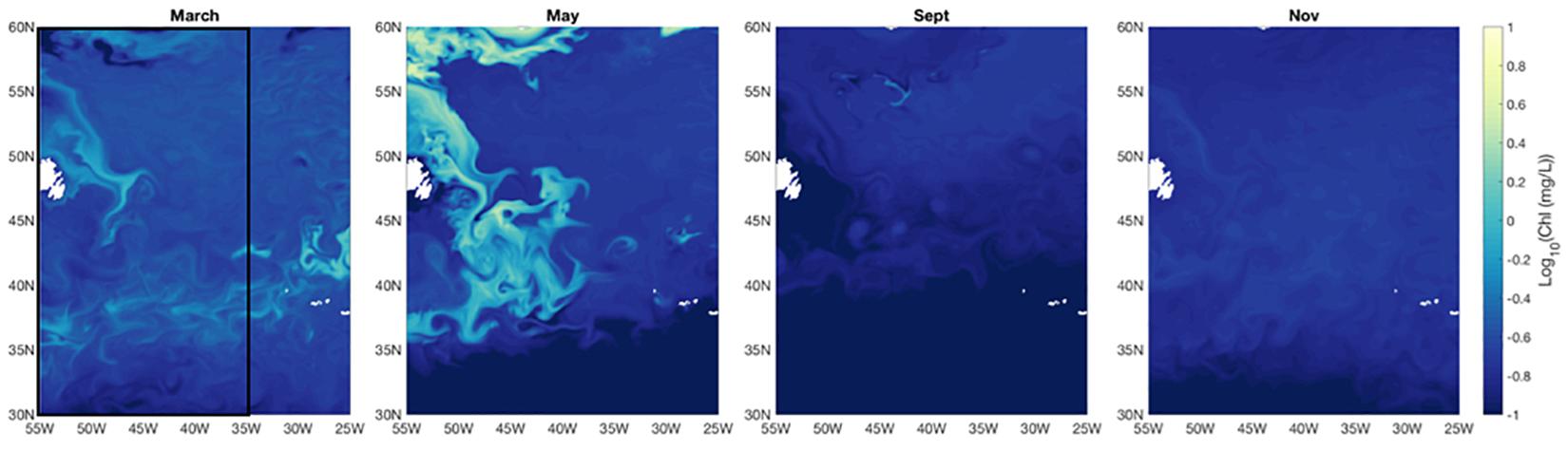
Figure 1. Monthly average Log₁₀ surface chlorophyll a concentration for March, May, September, and November from year 5 of the CESM simulation. Black rectangle on the western side of the left panel (March) indicates region displayed in Figures 3, 4.

FIGURE 2

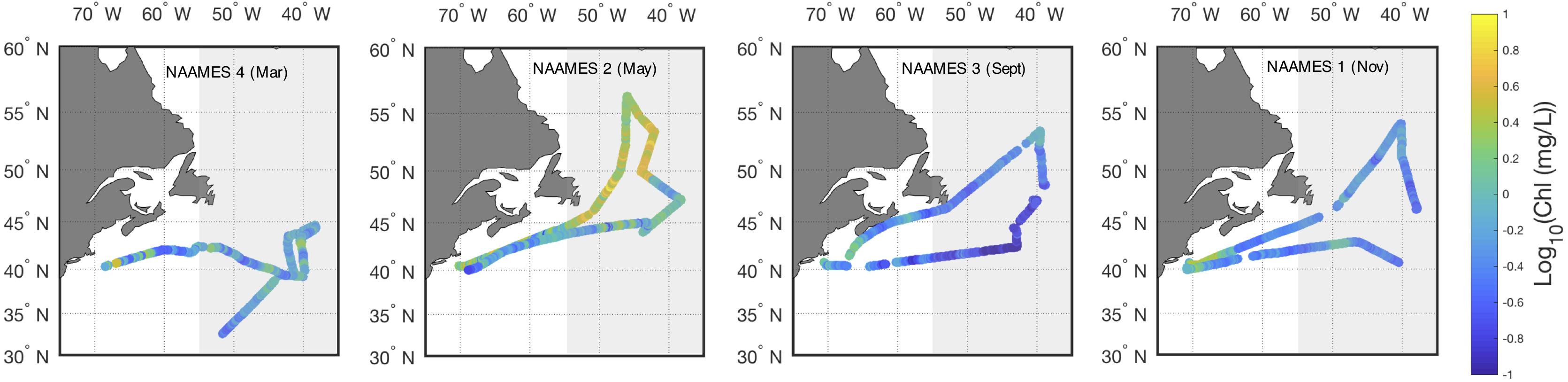
Figure 2. Field measured Log₁₀ surface chlorophyll a concentration for the four NAAMES campaigns, organized by month. Ship-based, underway measurements shown in closed circles. Grayed rectangle indicates grid region displayed in Figures 3, 4.

Geostatistical analysis of the CESM simulation shows that simulated mesoscale surface chlorophyll a variability is generally isotropic, meaning the magnitude of the resolved variability and the spatial scale (range) of variability are similar in the North-South and East-West directions (Figure 3). A seasonal cycle is detectable in the subpolar and temperate regions with higher resolved variability (sill) during the peak of the Spring bloom (average sill CV, of 0.54) compared to the Fall/Winter (average sill CV 0.04). The seasonal cycle is much less pronounced south of 35°N, corresponding to the oligotrophic region. Here the range in relative sill values in terms of CV is 0.03–0.19. Resolved variability is highest (CV near 1 in May) in the boundary current front around Newfoundland (Figure 4).

FIGURE 3

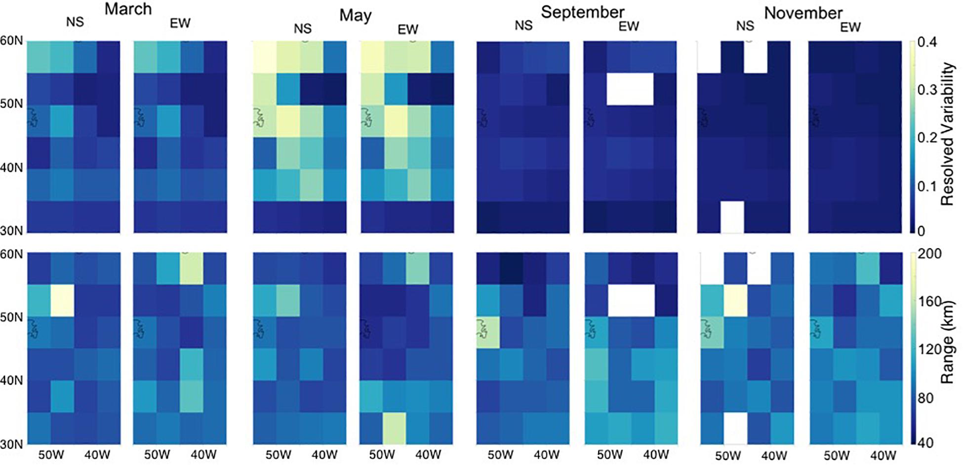
Figure 3. Geostatistical analysis of chlorophyll a from the Community Earth System Model (CESM). Simulated monthly average chlorophyll a resolved variability as computed from Eq. 2 (sill, top) and range (bottom) for March, May, September, and November in 5° × 5° grid boxes for the western North Atlantic sub-region denoted in Figure 1.

FIGURE 4

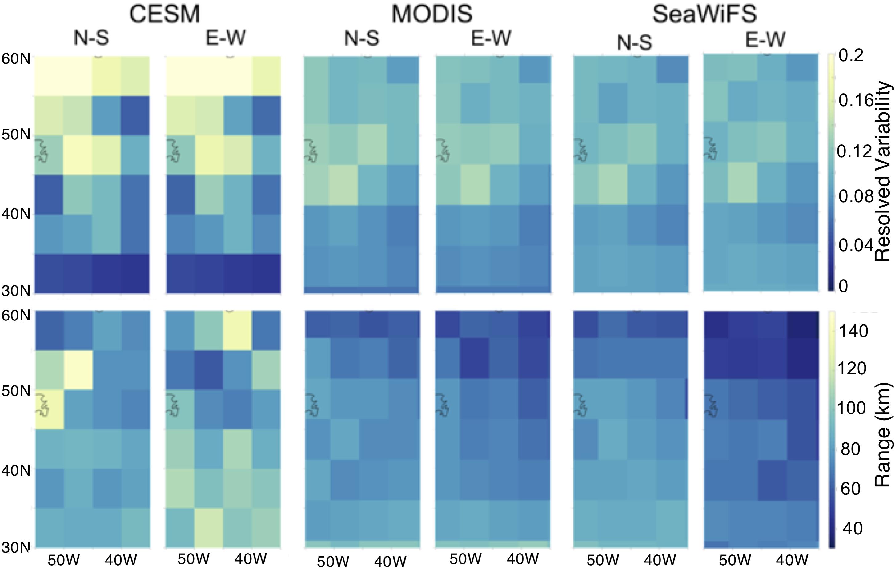
Figure 4. Geostatistical analysis of annual average surface chlorophyll a resolved variability as computed in Eq. 2 (sill, top) and range (bottom) from CESM, MODIS, and SeaWiFS in 5° × 5° grid boxes.

Both modeled and remotely sensed surface chlorophyll a show higher annually-averaged resolved variability in the northern portion of the study region as compared to the south, particularly north of 35° (Figure 4). The regional change in resolved sill is more pronounced in the CESM results than in satellite imagery, which shows a more gradual transition from a resolved sill of approximately 0.14 to 0.04. While we might expect the range or decorrelation length scale to be longer in the subtropics than in the subpolar region due to changes in physical stirring length scales with the Rossby radius (Doney et al., 2003), we see no clear difference in range in the model (annual mean 86 km North of 35°N and 88 km South of 35°) in contrast to a decreasing trend of range with latitude (Figure 4).

The patterns shown in the spatial maps were further analyzed by plotting the resolved arithmetic standard deviation from the resolved sill against the mean chlorophyll a concentration with lines of constant CV overlain (Figure 5; see Glover et al., 2018). Arithmetic standard deviation increases with mean chlorophyll a values for both observed and model data sets. The CV of ship-based field observations hovers around 0.3 for all cruise months and all locations along the cruise transect, relatively invariant of the mean chlorophyll a concentration. The CV of satellite remotely-sensed surface chlorophyll a is also uniform and slightly lower, approximately 0.2 for all months and all 5° × 5° grid boxes, and again does not correlate strongly with chlorophyll a concentration. For log-normal variables, CV is expected to depend on the variance of the log-transformed variable but not the mean data value [see Appendix, Glover et al. (2018)], similar to the pattern observed in the ship underway and remote sensing data.

FIGURE 5

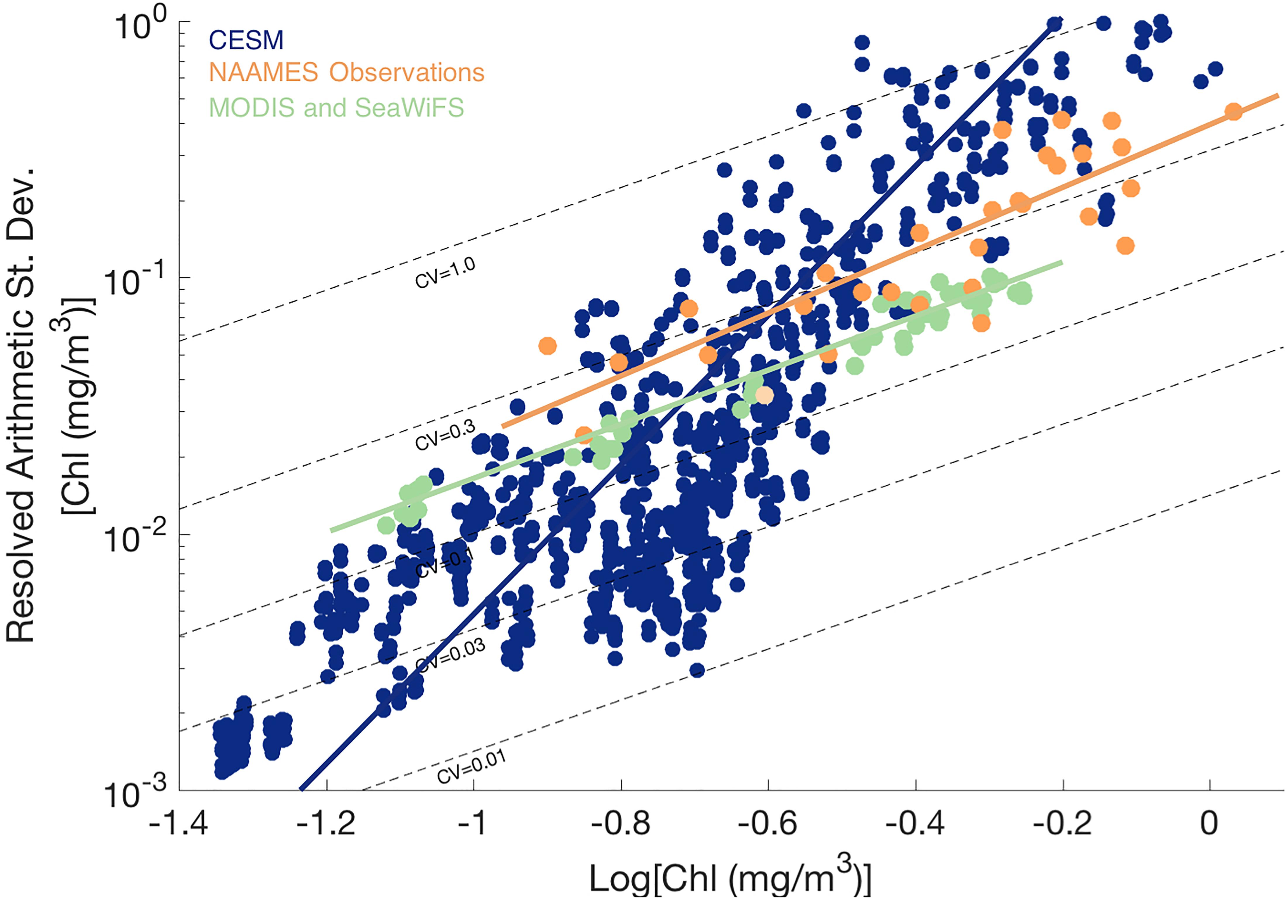
Figure 5. Resolved arithmetic standard deviation of surface chlorophyll a variability against Log₁₀ surface chlorophyll a concentration for CESM (blue), field observations from NAAMES underway ship data (orange), and MODIS and SeaWiFS satellite ocean color (green) over study region in the western North Atlantic. Dotted lines indicate lines of constant coefficient of variation (CV).

In contrast to the field and satellite observations, modeled surface chlorophyll mesoscale field has CVs ranging from 0.01 to 1.0, with CV generally increasing with the mean chlorophyll a value. Thus, when comparing CESM to observations, CESM CV is lower than expected at low chlorophyll a (in winter and the subtropical gyre) and higher than expected at high chlorophyll a (such as in the boundary front and in peak bloom conditions; see also Supplementary Figure 2).

Discussion and Conclusion

Improved measures of mesoscale biological variability in the surface ocean are needed both to address scientific questions and test the skill of eddy-resolving marine biophysical simulations. Geostatistical approaches, such as the variogram techniques used here, have some distinct advantages in that they can be applied to both 1-D and 2-D fields with data gaps (e.g., clouds in satellite remote sensing), partition resolved spatial variability from unresolved instrument and algorithm noise and sub sample-resolution scale biophysical processes, and provide a measure of the spatial correlation scale or range (Doney et al., 2003; Glover et al., 2018). Geostatistical techniques complement more eddy-centric compositing techniques (Chelton et al., 2011; Gaube et al., 2013; Rohr et al., 2020a, b) by incorporating frontal features as well as well-defined mesoscale eddies.

The geostatistical analysis of the NAAMES field observations from the western North Atlantic generally indicated similar patterns of resolved, mesoscale variability in surface chlorophyll a from ship-based underway data and satellite ocean color imagery, providing further support for the satellite results presented in Glover et al. (2018). Both the field and satellite data indicate relatively uniform, though somewhat offset, levels of CV (arithmetic standard deviation divided by the mean value) across a wide span in mean surface chlorophyll a concentrations, from oligotrophic to bloom conditions. The observational results indicate that the fractional variability of surface chlorophyll is similar across a wide range of ecosystem states, from oligotrophic to bloom conditions and across time from bloom initiation, peak, and termination; effectively, there is a similar normalized width of the local bell curve distribution for surface chlorophyll. The result of uniform CV is not simply an artifact of statistics for a log-normal variable but reflects an emergent property of marine biophysics likely arising from some combination of physical stirring and stimulation of biological production.

Differences in resolved variability across observational data sets may reflect differences in the fundamental spatial resolution of the sampling techniques and thus differences in the degree to which submesoscale variability is captured. The slightly higher mean CV for the underway ship data, when compared to MODIS and SeaWiFS, might arise because the ship observations are capturing more submesoscale variability. The influence of these small-scale processes is retained even after we interpolate the ship observations onto a 9 km grid, as indicated by the lack of change in resolved variability when going from raw data at approximately 0.3 km resolution to the gridded data (Supplementary Figure 1).

The eddy-resolving (1/10th degree horizontal resolution) CESM ocean bio-physical simulation (Harrison et al., 2018) created mesoscale biological patchiness at roughly the same magnitude and spatial decorrelation scales as observed in the field and with remote sensing. However, the simulation exhibits a striking difference from the field and remote sensing data in the relationship of the arithmetic standard deviation of mesoscale surface chlorophyll anomalies and the background mean field. In striking contrast to the relatively uniform CV found across a wide range of observed chlorophyll levels, the simulated CV of resolved mesoscale variability increases steeply with mean surface chlorophyll a levels. The model-resolved arithmetic standard deviation is biased low relative to observations while surface chlorophyll a concentrations are low and is too high where chlorophyll a is high.

Some of this discrepancy could arise because the underlying distribution of log chlorophyll a values in the region is further from “normal” for the model when compared to observations (Figure 6). However, within regional (5° × 5° bins) and temporal (monthly) domains relevant to the variogram analysis, the data is also approximately log-normal with the median skewness in each domain within ±1.6 (Supplementary Figure 3). Further, if we exclude results when the skewness is outside the bounds of ±1, consistent with best practices detailed in Kerry and Oliver (2007), the model’s variable CV with chlorophyll still holds (Supplementary Figure 4). While some of the issues likely reflect errors in the mean state of the model [see Harrison et al. (2018)], there are likely additional dynamical issues. The CV biases represent a clear deficiency in the mesoscale variability predicted by the model and one that would not be as obvious from simple visual comparisons of observed and simulated maps of the standard deviation of surface chlorophyll that combine mesoscale and mean field skill.

FIGURE 6

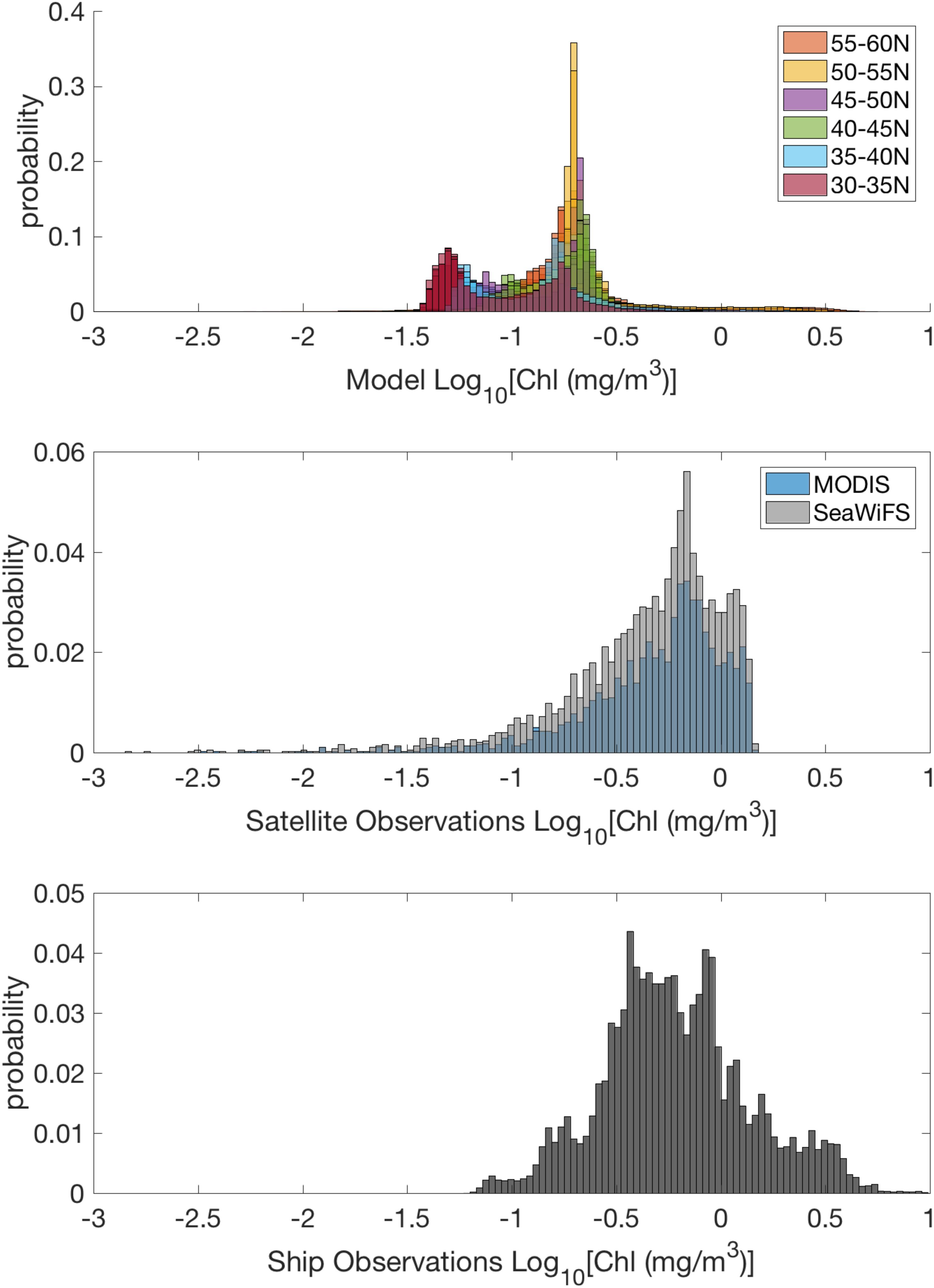
Figure 6. Normalized histograms of Log₁₀ Chlorophyll a concentration from the CESM model (top, colored by latitudinal band), satellites (middle), and ship observations (bottom).

The model resolution is 1/10th of a degree, which is approximately 9 km at this latitude in the temperate/subpolar North Atlantic. Thus, based on a regional Rossby radius of deformation of 10–35 km (Chelton et al., 1998), the model only resolved mid- to large mesoscale eddies and frontal features (10 s to 100 km) but did not capture smaller mesoscale and submesoscale processes. The effective spatial resolution of model biophysical dynamics may be larger than the nominal grid resolution such that smaller simulated mesoscale features generate overly weak chlorophyll anomalies in oligotrophic conditions. Also, ocean turbulence and biophysical variability extend well down into the submesoscale domain O(1–10 km) and smaller scales (Lévy, 2008; Lévy et al., 2018) that is not captured in the model. While the submesoscale variability in the observations would be partitioned into the variogram’s unresolved variance term, some of the submesoscale biophysical processes could be being rectified into the resolved mesoscale variability. Those unaccounted-for processes may be particularly important in generating spatial variability while background chlorophyll a is low, such as in fall/winter and in the oligotrophic gyre. This could point to problems with capturing physical nutrient supply mechanisms driving eddy-scale anomalies. In contrast, under high chlorophyll a conditions, the model arithmetic standard deviation is biased high. This could potentially be driven by boundary current processes rather than open-ocean mesoscale eddies.

As biophysical and biogeochemical ocean models continue to drill down to finer resolution, we need metrics to assess the skill of the predicted time/space variance fields, not simply the mean fields. In addition to standard bio-physical metrics such as mean state of bloom magnitude (e.g., Doney et al., 2009; Stow et al., 2009), we also need to include an assessment of a model’s ability to reproduce chlorophyll a variability seen in the real world, leveraging the wealth of satellite and autonomous platform data. Without this diagnostic, mesoscale simulations lose some of their utility in determining the mechanisms of bio-physical coupling driving chlorophyll a patchiness. The observation-tested simulations will also provide an avenue for developing improved parameterizations of sub-gridscale biophysical dynamics (e.g., nutrient injection by episodic upwelling events) that would complement efforts on dynamically consistent physical mixing parameterizations across resolution that are already under development (e.g., Jansen et al., 2019).

Data Availability Statement

Satellite data are available from https://oceancolor.gsfc.nasa.gov/ NASA’s OceanColor website. Ship-based data can be found in the SeaBASS data repository at https://seabass.gsfc.nasa.gov/experiment/NAAMES. The outputsfrom CESM simulation are available on request to ML.

Author Contributions

RE and SD designed the study and analyzed the data. DG provided satellite results and statistical expertise. ML performed the CESM model simulation. IL provided technical assistance with analysis of model data. AC processed and prepared all ship-based chlorophyll data. RE and SD prepared the manuscript with contributions from all co-authors. All authors contributed to the article and approved the submitted version.

Funding

This work was supported in part by the National Aeronautics and Space Administration (NASA) as part of the North Atlantic Aerosol and Marine Ecosystems Study (NAAMES; NASA grant 80NSSC18K0018). The CESM project is supported by the National Science Foundation and the Office of Science (BER) of the United States Department of Energy. Computing resources were provided by the Climate Simulation Laboratory at NCAR’s Computational and Information Systems Laboratory (CISL), sponsored by the National Science Foundation and other agencies. This research was enabled by CISL compute and storage resources.

Conflict of Interest

The authors declare that the research was conducted in the absence of any commercial or financial relationships that could be construed as a potential conflict of interest.

Acknowledgments

The authors gratefully acknowledge the efforts of all the science party and crew during the NAAMES ship and aircraft campaigns.

Supplementary Material

The Supplementary Material for this article can be found online at: https://www.frontiersin.org/articles/10.3389/fmars.2021.612764/full#supplementary-material

References

Behrenfeld, M. J., Moore, R. H., Hostetler, C. A., Graff, J., Gaube, P., Russell, L. M., et al. (2019). The North Atlantic aerosol and marine ecosystem study (NAAMES): science motive and mission overview. Front. Mar. Sci. 6:122. doi: 10.3389/fmars.2019.00122

CrossRef Full Text | Google Scholar

Bonan, G. B., and Doney, S. C. (2018). Climate, ecosystems, and planetary futures: the challenge to predict life in Earth system models. Science 359:eaam8328. doi: 10.1126/science.aam8328

PubMed Abstract | CrossRef Full Text | Google Scholar

Bryan, F. O., Hecht, M. W., and Smith, R. D. (2007). Resolution convergence and sensitivity studies with North Atlantic circulation models. Part I: The western boundary current system. Ocean Model. 16, 141–159. doi: 10.1016/j.ocemod.2006.08.005

CrossRef Full Text | Google Scholar

Campbell, J. W. (1995). The lognormal distribution as a model for bio-optical variability in the sea. J. Geophys. Res. 100:13237. doi: 10.1029/95JC00458

CrossRef Full Text | Google Scholar

Capotondi, A., Jacox, M., Bowler, C., Kavanaugh, M., Lehodey, P., Barrie, D., et al. (2019). Observational needs supporting marine ecosystems modeling and forecasting: from the global ocean to regional and coastal systems. Front. Mar. Sci. 6:623. doi: 10.3389/fmars.2019.00623

CrossRef Full Text | Google Scholar

Chelton, D. B., deSzoeke, R. A., Schlax, M. G., El Naggar, K., and Siwertz, N. (1998). Geographical variability of the first baroclinic rossby radius of deformation. J. Phys. Oceanogr. 28, 433–460.

Google Scholar

Chelton, D. B., Gaube, P., Schlax, M. G., Early, J. J., and Samelson, R. M. (2011). The influence of nonlinear mesoscale eddies on near-surface oceanic chlorophyll. Science 334, 328–332. doi: 10.1126/science.1208897

PubMed Abstract | CrossRef Full Text | Google Scholar

Clark, I. (1987). Practical Geostatics. London: Elsevier Applied Science.

Google Scholar

Clayton, S., Dutkiewicz, S., Jahn, O., Hill, C., Heimbach, P., and Follows, M. J. (2017). Biogeochemical versus ecological consequences of modeled ocean physics. Biogeosciences 14, 2877–2889. doi: 10.5194/bg-14-2877-2017

CrossRef Full Text | Google Scholar

Cressie, N. A. C. (1993). Statistics for Spatial Data, Revised Edition. New York, NY: Wiley.

Google Scholar

Currie, W. J. S., and Roff, J. C. (2006). Plankton are not passive tracers: Plankton in a turbulent environment. J. Geophys. Res. 111:C05S07. doi: 10.1029/2005JC002967

CrossRef Full Text | Google Scholar

Della Penna, A., and Gaube, P. (2019). Overview of (Sub)mesoscale ocean dynamics for the NAAMES field program. Front. Mar. Sci. 6:384. doi: 10.3389/fmars.2019.00384

CrossRef Full Text | Google Scholar

Denman, K. L., and Abbott, M. R. (1988). Time evolution of surface chlorophyll patterns from cross-spectrum analysis of satellite color images. J. Geophys. Res. 93:6789. doi: 10.1029/JC093iC06p06789

CrossRef Full Text | Google Scholar

Denman, K. L., and Abbott, M. R. (1994). Time scales of pattern evolution from cross-spectrum analysis of advanced very high resolution radiometer and coastal zone color scanner imagery. J. Geophys. Res. 99:7433. doi: 10.1029/93JC02149

CrossRef Full Text | Google Scholar

Denman, K. L., and Freeland, H. J. (1985). Correlation scales, objective mapping and a statistical test of geostrophy over the continental shelf. J. Mar. Res. 43, 517–539. doi: 10.1357/002224085788440402

CrossRef Full Text | Google Scholar

Denman, K. L., and Platt, T. (1976). The variance spectrum of phytoplankton in a turbulent ocean. J. Mar. Res. 34, 593–601.

Google Scholar

Doney, S. C. (1999). Major challenges confronting marine biogeochemical modeling. Global Biogeochem. Cycles 13, 705–714. doi: 10.1029/1999GB900039

CrossRef Full Text | Google Scholar

Doney, S. C., Glover, D. M., McCue, S. J., and Fuentes, M. (2003). Mesoscale variability of sea-viewing wide field-of-view sensor (SeaWiFS) satellite ocean color: global patterns and spatial scales: mesoscale variability of satellite ocean color. J. Geophys. Res. Oceans 108:3024. doi: 10.1029/2001JC000843

CrossRef Full Text | Google Scholar

Doney, S. C., Lima, I., Moore, J. K., Lindsay, K., Behrenfeld, M. J., Westberry, T. K., et al. (2009). Skill metrics for confronting global upper ocean ecosystem-biogeochemistry models against field and remote sensing data. J. Mar. Syst. 76, 95–112. doi: 10.1016/j.jmarsys.2008.05.015

CrossRef Full Text | Google Scholar

Gaube, P., Chelton, D. B., Strutton, P. G., and Behrenfeld, M. J. (2013). Satellite observations of chlorophyll, phytoplankton biomass, and Ekman pumping in nonlinear mesoscale eddies: PHYTOPLANKTON AND EDDY-EKMAN PUMPING. J. Geophys. Res. Oceans 118, 6349–6370. doi: 10.1002/2013JC009027

CrossRef Full Text | Google Scholar

Gent, P. R., and Mcwilliams, J. C. (1990). Isopycnal mixing in ocean circulation models. J. Phys. Oceanogr. 20, 150–155.

Google Scholar

Glover, D. M., Doney, S. C., Oestreich, W. K., and Tullo, A. W. (2018). Geostatistical analysis of mesoscale spatial variability and error in SeaWiFS and MODIS/Aqua global ocean color data: seawifs and modis mesoscale variability. J. Geophys. Res. Oceans 123, 22–39. doi: 10.1002/2017JC013023

CrossRef Full Text | Google Scholar

Gower, J. F. R., Denman, K. L., and Holyer, R. J. (1980). Phytoplankton patchiness indicates the fluctuation spectrum of mesoscale oceanic structure. Nature 288, 157–159. doi: 10.1038/288157a0

CrossRef Full Text | Google Scholar

Harrison, C. S., Long, M. C., Lovenduski, N. S., and Moore, J. K. (2018). Mesoscale effects on carbon export: a global perspective. Glob. Biogeochem. Cycles 32, 680–703. doi: 10.1002/2017GB005751

CrossRef Full Text | Google Scholar

Hurlburt, H., Brassington, G., Drillet, Y., Kamachi, M., Benkiran, M., Bourdallé-Badie, R., et al. (2009). High-resolution global and basin-scale ocean analyses and forecasts. Oceanog. 22, 110–127. doi: 10.5670/oceanog.2009.70

CrossRef Full Text | Google Scholar

Jansen, M. F., Adcroft, A., Khani, S., and Kong, H. (2019). Toward an energetically consistent, resolution aware parameterization of ocean mesoscale eddies. J. Adv. Model. Earth Syst. 11, 2844–2860. doi: 10.1029/2019MS001750

CrossRef Full Text | Google Scholar

Journel, A. G., and Huijbregts, C. J. (1978). Mining Geostatistics. London: Academic Press.

Google Scholar

Kerry, R., and Oliver, M. A. (2007). Determining the effect of asymmetric data on the variogram. I. Underlying asymmetry. Comput. Geosci. 33, 1212–1232. doi: 10.1016/j.cageo.2007.05.008

CrossRef Full Text | Google Scholar

Lévy, M. (2008). “The modulation of biological production by oceanic mesoscale turbulence,” in Transport and Mixing in Geophysical Flows Lecture Notes in Physics, eds J. B. Weiss and A. Provenzale (Berlin, Heidelberg: Springer Berlin Heidelberg), 219–261. doi: 10.1007/978-3-540-75215-8_9

CrossRef Full Text | Google Scholar

Lévy, M., and Franks, P. J. S., and Smith, K. S. (2018). The role of submesoscale currents in structuring marine ecosystems. Nat. Commun. 9:4758. doi: 10.1038/s41467-018-07059-3

PubMed Abstract | CrossRef Full Text | Google Scholar

Mackas, D. L., Denman, K. L., and Abbott, M. R. (1985). Plankton patchiness: biology in the physical vernacular. Bull. Mar. Sci. 37, 652–674.

Google Scholar

Marcotte, D. (1996). Fast variogram computation with FFT. Comput. Geosci. 22, 1175–1186. doi: 10.1016/S0098-3004(96)00026-X

CrossRef Full Text | Google Scholar

McGillicuddy, D. J. (2016). Mechanisms of physical-biological-biogeochemical interaction at the oceanic mesoscale. Annu. Rev. Mar. Sci. 8, 125–159. doi: 10.1146/annurev-marine-010814-015606

PubMed Abstract | CrossRef Full Text | Google Scholar

McGillicuddy, D. J., Anderson, L. A., Doney, S. C., and Maltrud, M. E. (2003). Eddy-driven sources and sinks of nutrients in the upper ocean: results from a 0.1° resolution model of the North Atlantic: EDDY-DRIVEN SOURCES AND SINKS OF NUTRIENTS. Glob. Biogeochem. Cycles 17:1035. doi: 10.1029/2002GB001987

CrossRef Full Text | Google Scholar

McGillicuddy, D. J., and Franks, P. J. S. (2019). “Models of Plankton patchiness,” in Encyclopedia of Ocean Sciences, eds J. K. Cochran, H. J. Bokuniewicz, and P. L. Yager (Amsterdam: Elsevier), 536–546.

Google Scholar

Moore, J. K., Lindsay, K., Doney, S. C., Long, M. C., and Misumi, K. (2013). Marine ecosystem dynamics and biogeochemical cycling in the community earth system model [CESM1(BGC)]: comparison of the 1990s with the 2090s under the RCP4.5 and RCP8.5 scenarios. J. Clim. 26, 9291–9312. doi: 10.1175/JCLI-D-12-00566.1

CrossRef Full Text | Google Scholar

O’Reilly, J., Mueller, J. L., Michell, B. G., Kahru, M., Chavez, F. P., Strutton, P., et al. (2000). SeaWIFS postlaunch calibration and validation analyses, Part 3. NASA Tech. Memo. 2000–206892 11:49.

Google Scholar

Oschlies, A., and Garçon, V. (1998). Eddy-induced enhancement of primary production in a model of the North Atlantic Ocean. Nature 394, 266–269. doi: 10.1038/28373

CrossRef Full Text | Google Scholar

Platt, T. (1972). Local phytoplankton abundance and turbulence. Deep Sea Res. Oceanogr. Abstracts 19, 183–187. doi: 10.1016/0011-7471(72)90029-0

CrossRef Full Text | Google Scholar

Roesler, C. S., and Barnard, A. H. (2013). Optical proxy for phytoplankton biomass in the absence of photophysiology: rethinking the absorption line height. Methods Oceanogr. 7, 79–94. doi: 10.1016/j.mio.2013.12.003

CrossRef Full Text | Google Scholar

Rohr, T., Harrison, C., Long, M. C., Gaube, P., and Doney, S. C. (2020a). Eddy−modified iron, light, and phytoplankton cell division rates in the simulated southern ocean. Glob. Biogeochem. Cycles 34:e2019GB006380. doi: 10.1029/2019GB006380

CrossRef Full Text | Google Scholar

Rohr, T., Harrison, C., Long, M. C., Gaube, P., and Doney, S. C. (2020b). The simulated biological response to southern ocean eddies via biological rate modification and physical transport. Glob. Biogeochem. Cycles 34:e2019GB006385. doi: 10.1029/2019GB006385

CrossRef Full Text | Google Scholar

Slade, W. H., Boss, E., Dall’Olmo, G., Langner, M. R., Loftin, J., Behrenfeld, M. J., et al. (2010). Underway and moored methods for improving accuracy in measurement of spectral particulate absorption and attenuation. J. Atmos. Oceanic Technol. 27, 1733–1746. doi: 10.1175/2010JTECHO755.1

CrossRef Full Text | Google Scholar

Smith, R., Jones, P., Briegleb, B., Bryan, F., Danabasoglu, G., Dennis, J., et al. (2010). The Parallel Ocean Program (POP) Reference Manual Ocean Component of the Community Climate System Model (CCSM) and Community Earth System Model (CESM). Available online at: http://n2t.net/ark:/85065/d70g3j4h (accessed March 23, 2010).

Google Scholar

Steele, J. H., and Henderson, E. W. (1979). Spatial patterns in North Sea plankton. Deep Sea Res. A Oceanogr. Res. Pap. 26, 955–963. doi: 10.1016/0198-0149(79)90107-9

CrossRef Full Text | Google Scholar

Stow, C. A., Jolliff, J., McGillicuddy, D. J., Doney, S. C., Allen, J. I., Friedrichs, M. A. M., et al. (2009). Skill assessment for coupled biological/physical models of marine systems. J. Mar. Syst. 76, 4–15. doi: 10.1016/j.jmarsys.2008.03.011

PubMed Abstract | CrossRef Full Text | Google Scholar

Tortell, P. D., and Long, M. C. (2009). Spatial and temporal variability of biogenic gases during the Southern Ocean spring bloom. Geophys. Res. Lett. 36:L01603. doi: 10.1029/2008GL035819

CrossRef Full Text | Google Scholar

Weber, L. H., El-Sayed, S. Z., and Hampton, I. (1986). The variance spectra of phytoplankton, krill and water temperature in the Antarctic Ocean south of Africa. Deep Sea Res. A Oceanogr. Res. Pap. 33, 1327–1343. doi: 10.1016/0198-0149(86)90039-7

CrossRef Full Text | Google Scholar

Yang, B., Boss, E. S., Haëntjens, N., Long, M. C., Behrenfeld, M. J., Eveleth, R., et al. (2020). Phytoplankton phenology in the North Atlantic: insights from profiling float measurements. Front. Mar. Sci. 7:139. doi: 10.3389/fmars.2020.00139

CrossRef Full Text | Google Scholar

Yoder, J. A., McClain, C. R., Blanton, J. O., and Oeymay, L.-Y. (1987). Spatial scales in CZCS-chlorophyll imagery of the southeastern U.S. continental shelf1: spatial scales in CZCS Chi. Limnol. Oceanogr. 32, 929–941. doi: 10.4319/lo.1987.32.4.0929

CrossRef Full Text | Google Scholar