Mixing in the Tyrrhenian Interior Due to Thermohaline Staircases

Introduction

Thermohaline staircases are a characteristic of the central part of the Tyrrhenian Sea, the deepest and most isolated basin of the Western Mediterranean (Figure 1). They are an alternation of homogeneous temperature and salinity layers, and high gradient interfaces, the thicknesses of which can reach several hundreds and tens of meters, respectively. Observed more frequently in the depth range of 600–2500 m (e.g., Zodiatis and Gasparini, 1996), such staircases extended up to 3000 m after the year 2010 (Durante et al., 2019). It is worth noting that among the Mediterranean sub-basins, the Tyrrhenian Sea is the most susceptible to salt fingering, and the one with the strongest likelihood of sustaining the processes leading to their formation (Meccia et al., 2016).

FIGURE 1

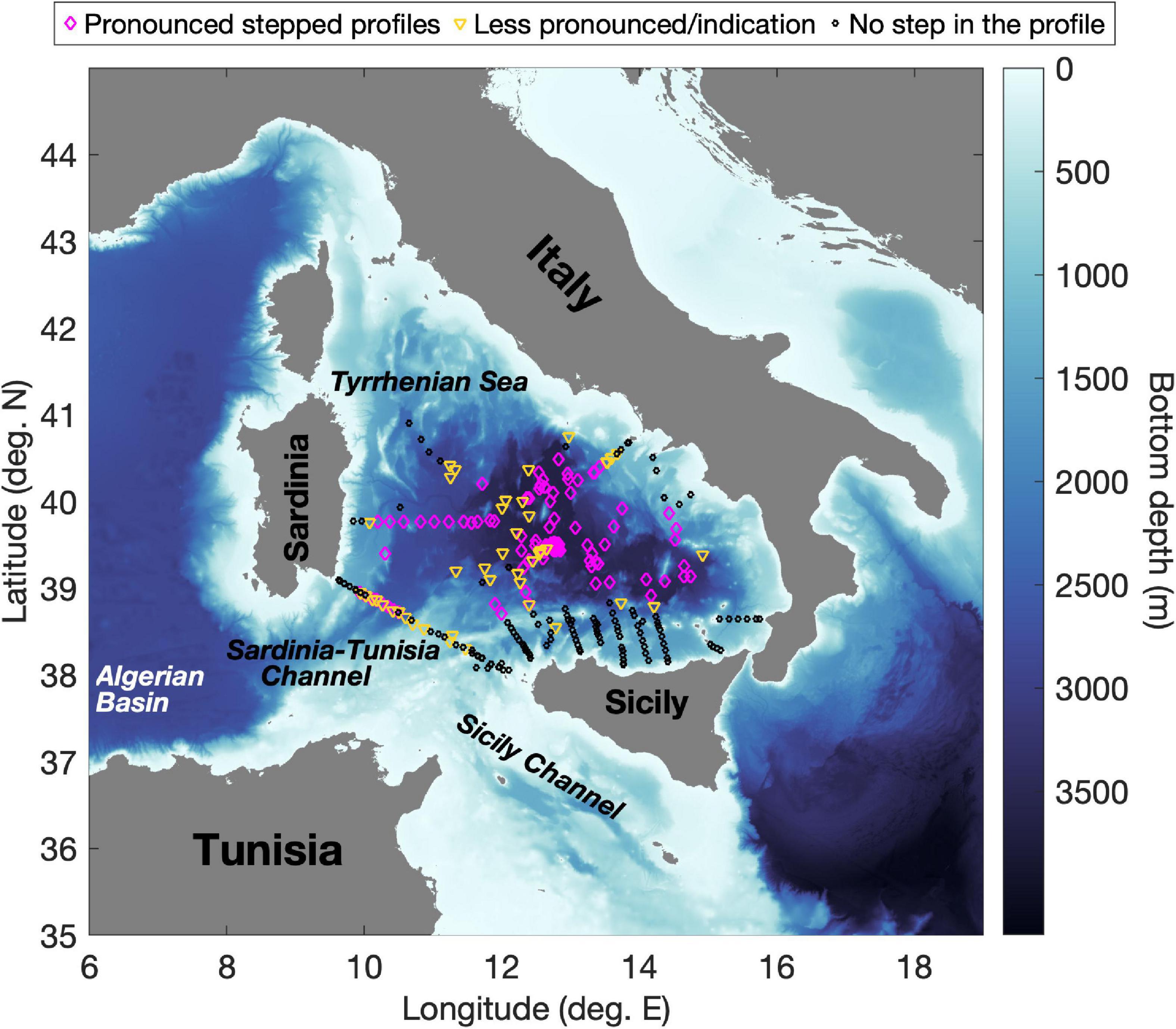
Figure 1. The Tyrrhenian Sea (Western Mediterranean); symbols denote stations from Johannessen and Lee (1974), Molcard and Williams (1975), Zodiatis and Gasparini (1996), Sparnocchia et al. (1999), Falco et al. (2016), Durante et al. (2019), Sparnocchia and Borghini (2019), and Taillandier et al. (2020), indicating the locations where well-defined/less-defined stepped profiles or profiles with no indication of steps were reported. The bathymetry is that of the GEBCO Bathymetric Compilation Group (2019), and the colormap used is from Thyng et al. (2016).

Documented for the first time by Johannessen and Lee (1974), these peculiar structures have been the subject of various studies that have demonstrated their persistence over time (Falco et al., 2016; Durante et al., 2019; Taillandier et al., 2020) as well as their spatial coherence (Molcard and Williams, 1975; Zodiatis and Gasparini, 1996; Buffett et al., 2017). Zodiatis and Gasparini (1996) in particular, using their extensive dataset which covered a large part of the southern Tyrrhenian Sea, were able to demonstrate that the staircase phenomenon affects at least 22% of the basin with a lateral coherence of 150 km, and is more pronounced (thicker mixed layers, thinner interfaces with maximum gradients and a larger number of steps) in its deeper part. This is also evident from the distribution of profile types taken from the literature in Figure 1. Moving toward the basin’s periphery, the structures become weaker, and finally disappear completely. This feature of the structures is consistent with the dynamics of the basin which increases from the center toward the borders where advection is prevalent and diffusive convection is prevented (Astraldi and Gasparini, 1994; Zodiatis and Gasparini, 1996).

The Tyrrhenian water column is mainly a three-layer system consisting of the surface Atlantic Water (AW), the Levantine Intermediate Water (LIW) and the Tyrrhenian Deep Water (TDW). The LIW is generated in the Eastern Mediterranean and is identified by an associated salinity maximum. It enters the Tyrrhenian Sea from the Sicily Channel. A major part turns right and flows directly eastward following the northern coast of Sicily, circulating cyclonically within the basin along the boundaries in the 200–700 m depth range roughly. Reaching the eastern coast of Sardinia, it flows southward to finally exit the Tyrrhenian toward the Western Mediterranean (Béranger et al., 2004). The TDW is the product of the mixing between the Western Mediterranean Deep Water (WMDW) entering the Tyrrhenian Sea via the Sardinia-Tunisia Channel and waters of eastern Mediterranean origin, i.e., LIW and Eastern Mediterranean Deep Waters (Sparnocchia et al., 1999; Millot and Taupier-Letage, 2005). Fuda et al. (2002) hypothesized that water denser than TDW found in the deep Tyrrhenian (2000–3500 m) might form locally occasionally, but this hypothesis was not supported by further observations. The circulation of the TDW is not well-characterized due to the lack of data (Vetrano et al., 2010) but is expected to be cyclonic along-slope due to the Coriolis effect, tracing a basin-wide gyre before leaving through a southwest passage close to Sardinia (sill at ∼2000 m) (Millot and Taupier-Letage, 2005).

Lateral exchange processes between the boundary currents and the interior of the basin have been reported by Zodiatis and Gasparini (1996). More recent studies (Budillon et al., 2009; Vetrano et al., 2010) have revealed a complex circulation in the south-eastern part of the basin, with meanders and some persistent and transient cyclonic and anticyclonic structures involving the surface and intermediate layers. These exchange processes are responsible for lateral intrusions which supply the central part of the basin with warmer and saltier water, thus supporting the staircases. Lateral intrusions which alter the stratification of otherwise homogeneous steps in the form of local inversions of temperature and salinity with increasing depth are also sometimes observed (Zodiatis and Gasparini, 1996, their Figure 5; Merryfield, 2000). The continuous lateral input of warm, salty water and the weak dynamics of the basin in the deep layers (Hopkins, 1988; Astraldi and Gasparini, 1994; Zodiatis and Gasparini, 1996) contribute to maintaining the general pattern of the established structure of the relevant portion of the water column over time, though specific characteristics may change somewhat leading to slightly differing shapes of profiles between one observation and another (Durante et al., 2019).

In recent years, the LIW has undergone significant warming and an increase in salinity (Schroeder et al., 2017, 2020), which should therefore have increased its contribution to the salt fingering processes in the Tyrrhenian basin. Furthermore, following the Western Mediterranean Transition (WMT), a new warmer, saltier and denser Western Mediterranean Deep Water (nWMDW) has formed (Schroeder et al., 2008) that has progressively spread from its region of origin along routes to Gibraltar and the Tyrrhenian Sea (Schroeder et al., 2016). Entering the Tyrrhenian Sea, the nWMDW has a lower temperature and salinity than the resident deep waters but a higher density that causes it to cascade down to the bottom of the basin and settle under the deep water already present there (see Figure 2C in Schroeder et al., 2016). According to Durante et al. (2019), this new water at the bottom introduces an additional demand for downward fluxes of heat and salt, enhancing salt fingering processes.

Salt fingers reinforce heat and salt fluxes in the open ocean, strongly contributing to the diapycnal vertical mixing (St. Laurent and Schmitt, 1999; Schmitt et al., 2005). They are an effective mixing mechanism in the deep water of the Western Mediterranean (Bryden et al., 2014), and are believed to be the cause of the observed increases in deep water temperature and salinity over the past 50 years along with deep water formation events (Borghini et al., 2014). However, calculating their contribution to the vertical transport of heat and salt from hydrological observations is not easy as this is usually based on approximations of relative flux laws that have not been definitively verified yet as applicable for every situation observed in the ocean.

The laboratory-derived flux laws, also known as the 4/3 flux laws, relate the salt finger fluxes to the 4/3 power law of the difference in salinity across a fingering interface (ΔS^4/3) and the density ratio (Turner, 1967; Linden, 1973; Schmitt, 1979; McDougall and Taylor, 1984). But they have been found to overestimate fluxes by more than an order of magnitude (Gregg and Sanford, 1987; Lueck, 1987; Schmitt, 1988) because the high-gradient interfaces observed at sea are thicker than laboratory predictions for them.

Kunze (1987) was the first to propose a model of heat and salt fluxes for finite-length salt fingers, such as those found in observations. His main challenge was properly understanding the length and lengthening in time of the fingers. Since the observed interfaces are thicker than the maximum finger length (tens of cm) predicted by the 4/3 flux laws, they must either consist of several layers of fingering zones separated by convective regions (as suggested by Linden, 1978) or be a statistical ensemble of growing fingers. Thus, the laboratory flux laws that apply to interfaces with only one layer of salt fingers give incorrect fluxes for many of the steps observed in the ocean. In his formulation, Kunze (1987) gave an alternative argument in support of the Stern number constraint for collective instability (Stern, 1969) and a solution for both thin (∼30 cm) and thicker interfaces. This model reproduces laboratory behavior if a single finger fills the entire interface and is more suitable for thick interfaces, typical of oceanic thermohaline staircases, reproducing fluxes over an order of magnitude lower than the those predicted by the 4/3 flux laws.

More recently, Radko and Smith (2012), questioning whether the Stern (1969) and Kunze (1987) hypothesis could be extended to include the case of the very low Stern numbers associated with many of the laboratory experiments, emphasized the role played by secondary instabilities of the salt fingers. These typically grow much faster than the collective instability modes and are independent of the specific values of the Stern number (Holyer, 1984). Their theory, which assumes that the fully developed equilibrium state is characterized by the comparable growth rates of primary and secondary instabilities, leads to a set of equations for the non-dimensional heat and salt fluxes and the flux ratio.

Direct numerical simulations (Radko, 2003, 2005; Radko et al., 2014b) show that the equilibrium structure of a staircase is achieved by a sequence of merging events initially involving relatively thin and unsteady layers generated by instabilities within a smooth stratification. These layers merge continuously, building up the average layer thickness to a maximum value whereupon the equilibrium structure of the staircase is reached. Most oceanic staircases are in the quasi-equilibrium state, and the initial phase of formation of layers from smooth stratification and their systematic thickening subsequently have not been recorded. Nonetheless, in the case of the Tyrrhenian staircases, the varying numbers of such layers observed at different times, the diversity encountered in their sizes and the shapes of their interfaces (which sometimes include small, homogeneous and relatively thick sub-layers) suggest that some process of merging actually occurs (Durante et al., 2019).

Ma and Peltier (2021) further extended the Radko theory by simulating the formation and evolution of staircases starting from an inhomogeneous background stratification to better explain what happens in the real ocean. We will show later that, although they use different functions to represent the flux ratio, the parameterizations of Radko and Smith (2012) and Ma and Peltier (2021) produce nearly coincident salt and heat fluxes when applied to our dataset.

In this study, the Tyrrhenian staircase system presented by Durante et al. (2019) is examined in greater detail, particularly from the perspective of its evolution over time. Relevant fluxes of salt and heat have been calculated employing the parameterization of the Kunze (1987) model for thick interfaces proposed by Hebert (1988), as well as the Radko and Smith (2012) and the Ma and Peltier (2021) models (hereafter referred to as H88, RS12, and MP21, respectively). The main objective is to better formulate this system and assess its contribution to vertical mixing in the Tyrrhenian basin, paying attention also to the role played by the substructures observed inside the thick, layered interfaces. Our results have been evaluated by comparing them to those obtained from hydrological profiles in the same region by Zodiatis and Gasparini (1996) and Falco et al. (2016), the latter with the same parameterizations we use in this study. Another valuable source of comparison is the very recent study by Ferron et al. (2021), published in this issue. They estimate heat, salt and buoyancy fluxes using microstructure observations from four locations in the western Mediterranean, including our region in the Tyrrhenian Sea. Finally, we present a method for the semi-automatic detection of the boundaries of the interfaces in a stepped profile, specifically developed for our data, as an aid to extract information useful in the calculation of the associated heat and salt fluxes.

The paper is organized in the following way. In Section “Materials and Methods,” we present the data, the detection algorithm, the methods used for calculating heat and salt fluxes, and the comparison of the performances of the respective models underpinning the different sets of computations that were performed. In Section “Results,” we present an analysis of the long-term evolution of the Tyrrhenian staircase system and describe some of its salient features. We then present the results of the calculations of salt finger fluxes through interfaces, including an analysis of how they change when substructures are present. The two successive sections contain a discussion of the results and our overall conclusions, respectively.

Materials and Methods

Data

The dataset consists of a time series of vertical temperature and salinity profiles collected by the Consiglio Nazionale delle Ricerche (CNR) at a station located at a depth of about 3500 m in the central Tyrrhenian Sea (39.78083 deg N, 11.88333 deg E) over the period 2003–2016. This dataset has been presented and intensively studied in Durante et al. (2019), and is available on the open marine science data publication portal, SEANOE (Borghini et al., 2019). It contains 21 hydrological profiles, roughly one every six months with gaps in 2008 and 2009. The dataset can be considered highly homogeneous in terms of technical characteristics and quality. There are two reasons why this is so. One is that the instrument used to collect most of the profiles was the same Sea-Bird SBE 911plus Conductivity-Temperature-Depth (CTD) probe. The other is that the applied data qualification procedures were identical for every profile. The vertical profiles were collected with a sampling frequency of 24 Hz and an average probe descent rate of 1 m s^–1. The SBE 911plus CTD system mounts a SBE 3plus and a SBE 4 sensor for measuring temperature and conductivity, respectively, with corresponding manufacturer-declared accuracies of 0.001°C and 0.0003 S m^–1. These accuracies for the temperature and conductivity measurements are commensurate with an accuracy of roughly 0.003 in salinity (PSS-78). The temperature and conductivity sensors of the CTD probe were regularly calibrated at the NATO-CMRE Center in La Spezia until 2014, and subsequently by the manufacturer or by the OGS Oceanographic Calibration Center in Trieste. To verify the probe’s post-calibration performances for temperature and salinity measurements, it was often deployed with redundant temperature and conductivity sensors. In addition, in the specific case of salinity, probe readings were checked, and if necessary corrected, using values for the property obtained by analyzing water samples collected for this very purpose onboard with a Guildline Autosal or a Guildline Portasal bench salinometer. As a rule, the data acquired with the CTD probe were processed by means of the standard data processing package supplied by its manufacturer, Sea-Bird Scientific. In each profile, the measured temperature (ITS-90, °C) and salinity (PSS-78, practical salinity) data were averaged at every dbar in the vertical. The resulting values were used with the TEOS-10 software v3.06 (McDougall and Barker, 2011) to calculate the absolute salinity (SA) in g kg^–1 and the conservative temperature (CT) in °C, these variables being the best estimates for ocean temperature and salinity (Jackett et al., 2006; Millero et al., 2008; IOC et al., 2010). In the present version of the TEOS-10 software, the SA is obtained by multiplying the practical salinity by 1.004715428571429 g kg^–1.

Detection of Interfaces

To extract the upper and lower limits of the interfaces in a stepped profile, we developed an algorithm in Matlab which we applied below the LIW that we identified by the maximum SA value (SA_max). The entire procedure is summarized by the diagram in Figure 2 and explained below.

FIGURE 2

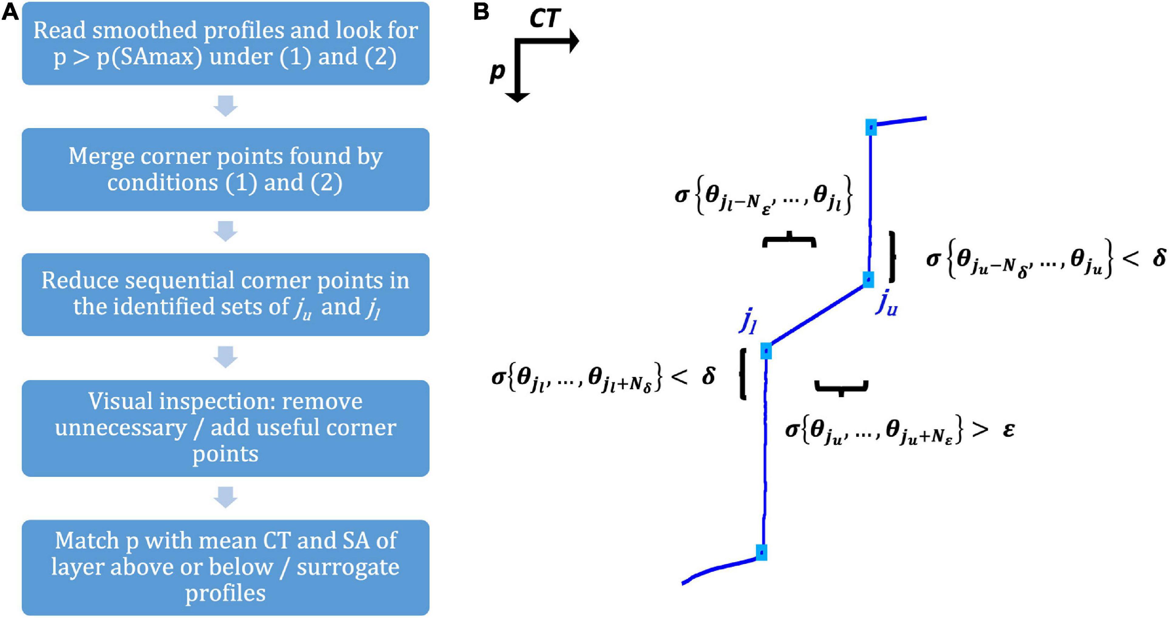
Figure 2. (A) Outline of the interface detection procedure, indicating the main steps. (B) Detail of a CT profile with staircases illustrating the conditions (1) and (2) explained in Section “Detection of Interfaces” used to detect corner points j_u and j_l; N_δ and N_ε are the set of points adjacent to points j_u and j_l where the two conditions apply.

The portion of the vertical profile below the LIW can be likened to an expression of a noisy piecewise function composed of two kinds of alternating subsections. The first kind has been defined by us as a “layer.” This subsection is characterized by a low variability in the property of interest (CT or SA) and a high variability in the pressure. The second one – which we have called an “interface” – is a subsection where the above situation is reversed, showing a high variability in properties and a low variability in the pressure. So, we based our algorithm on the following two criteria:

(i) the variability of CT (or SA) in the layers is smaller than a threshold value δ, and

(ii) the variability of CT (or SA) in the interfaces is larger than a threshold value ε.

The upper limit of an interface is a point j_u in the profile where it transforms from layer to interface. Similarly, the lower limit of an interface is a point j_l where the opposite occurs. Let N be the number of water column samples, θ = {θ₁,…,θ_N}, of the variable under examination (CT or SA). Then, if σ is its standard deviation in any given interval of pressure, j_u and j_l must satisfy the following conditions, namely:

$$\mathrm{\sigma }\{{\mathrm{\theta }}_{j_u-N_{\mathrm{\delta }}},\mathrm{\dots },{\mathrm{\theta }}_{j_u}\}<\mathrm{\delta }and\mathrm{\sigma }\{{\mathrm{\theta }}_{j_u},\mathrm{\dots },{\mathrm{\theta }}_{j_u+N_{\mathrm{\epsilon }}}\}>\mathrm{\epsilon }(1)$$

$$\mathrm{\sigma }\{{\mathrm{\theta }}_{j_l-N_{\mathrm{\epsilon }}},\mathrm{\dots },{\mathrm{\theta }}_{j_l}\}>\mathrm{\epsilon }and\mathrm{\sigma }\{{\mathrm{\theta }}_{j_l},\mathrm{\dots },{\mathrm{\theta }}_{j_l+N_{\mathrm{\delta }}}\}<\mathrm{\delta }(2)$$

where N_δ and Nε are the number of points adjacent to the corner points under scrutiny and are used to verify whether the conditions with respect to the δ and ε thresholds are met. To simplify the entire proceeding, the search for j_u and j_l (the corner points) was performed on the CT profiles only and, when identified, their corresponding pressure, CT and SA values were noted. To eliminate unwanted variability and make it easier for the automatic procedure to detect transitions from layers to interfaces and vice versa, we smoothed the original profiles by applying a moving average low-pass filter with a 15 dbar window. Following Durante et al. (2019), satisfactory values for δ and ε were set as 10^–4 °C and 10^–3 °C, respectively. After some sensitivity tests, we found that considering the closest 5 points (N_δ = 5) was sufficient to verify the desired low CT variability whereas the establishment of the opposite condition required addressing 10 points (Nε = 10). Furthermore, requisites (1) and (2) were both satisfied by multiple small groups of points spaced 1 dbar apart from each other. Subsequently, after the detection step, we tasked the algorithm with eliminating all the redundant points, keeping only the last of the sequential j_u and the first of the sequential j_l corner points because of their association with a greater ε variability. Finally, the ensuing derived profiles were superimposed on the corresponding recorded profiles, and the vertical alternation of interfaces and layers was verified by visual inspection. Any redundant corner points noticed again at this stage were eliminated by hand. Also, a few corner points that were missed by the algorithm were now added. To focus on the well-developed portion of a staircase conceived as a coherent succession of conspicuous homogeneous layers, we have selected those of thicknesses greater than 50 m. In doing so, we omit the small transient layers at the top of the staircases where the high variability suggests that there are no equilibrium conditions and therefore no justifiable way to apply the formulations (3), (4), and (5) described in the following subsection to calculate the relative heat and salt fluxes. We also ruled out the layers presenting inversions in the profiles of May 2010 (812–872 dbar and 895–1160 dbar), August 2010 (874–991 dbar), December 2010 (709–776 dbar), and May 2011 (699–752 dbar, 870–911 dbar, and 1075–1148 dbar). Finally, the small layers within the interfaces with substructures (see Section “Fluxes in Interfaces with a Stepped Substructure”) were ignored, and this type of interface was identified merely by its uppermost and lowermost limits while calculating fluxes. The results of the procedure are shown in Figure 3.

FIGURE 3

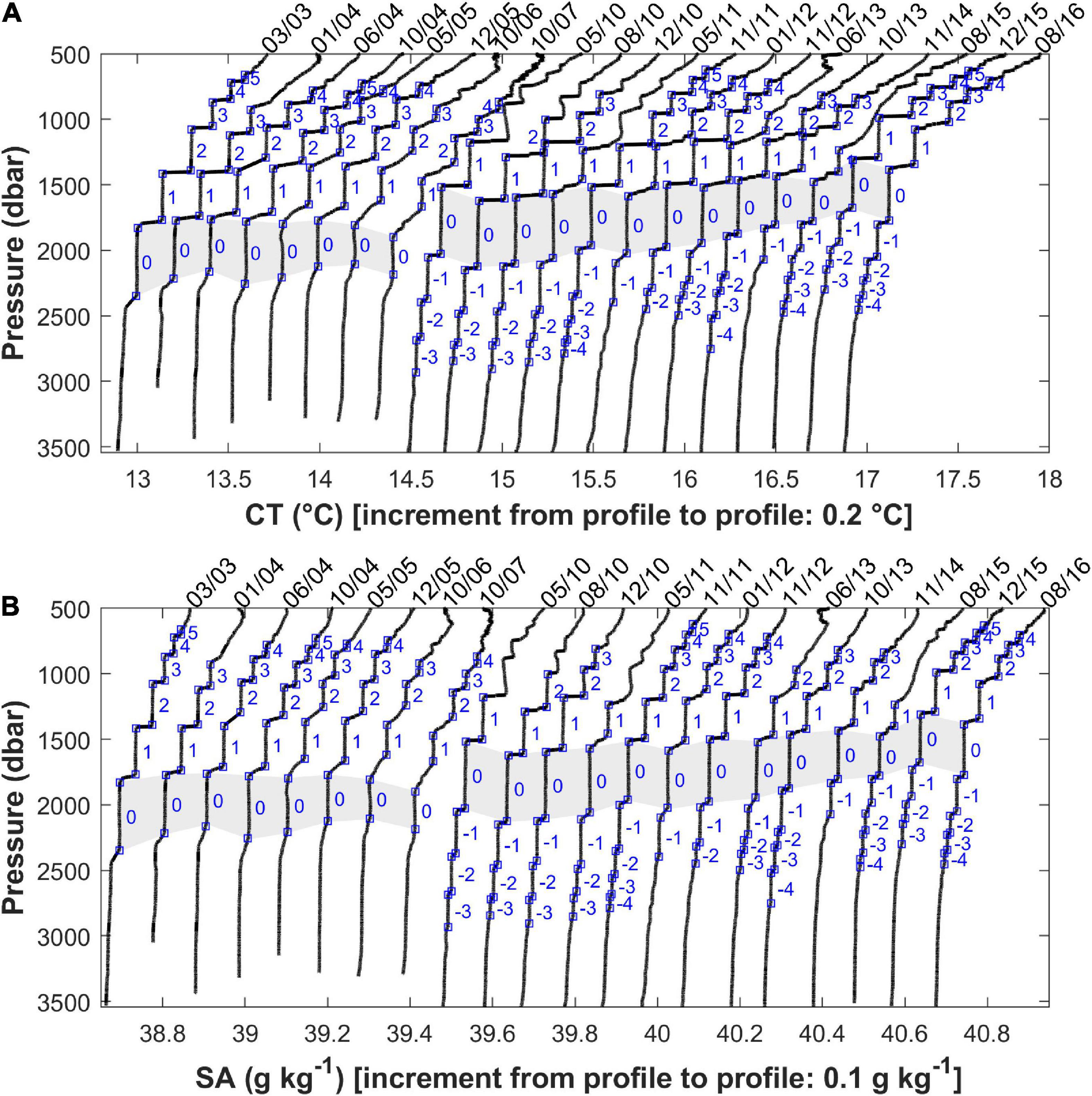
Figure 3. Original (i.e., not smoothed) temperature (A) and salinity (B) profiles from each cruise with the relevant selected corner points (blue squares) overlaid on each one; the temperature profiles are offset by 0.2°C and the salinity profiles by 0.1 g kg^–1 from cruise to cruise for better viewing. The gray band highlights the thickest layers found, numbered “0.” The layers above and below it are labeled sequentially with positive and negative numbers, respectively, in their natural order of succession going up or going down.

The last step was to set the values of CT and SA for the corner points as the mean values of CT and SA in the adjoining layers (the layer above for the j_u corner points and the layer below for the j_l corner points), leading to the surrogate profiles of Figure 4 which retain all the main properties of the thermohaline staircases and have been used to calculate the fluxes through the interfaces sandwiched between the main layers.

FIGURE 4

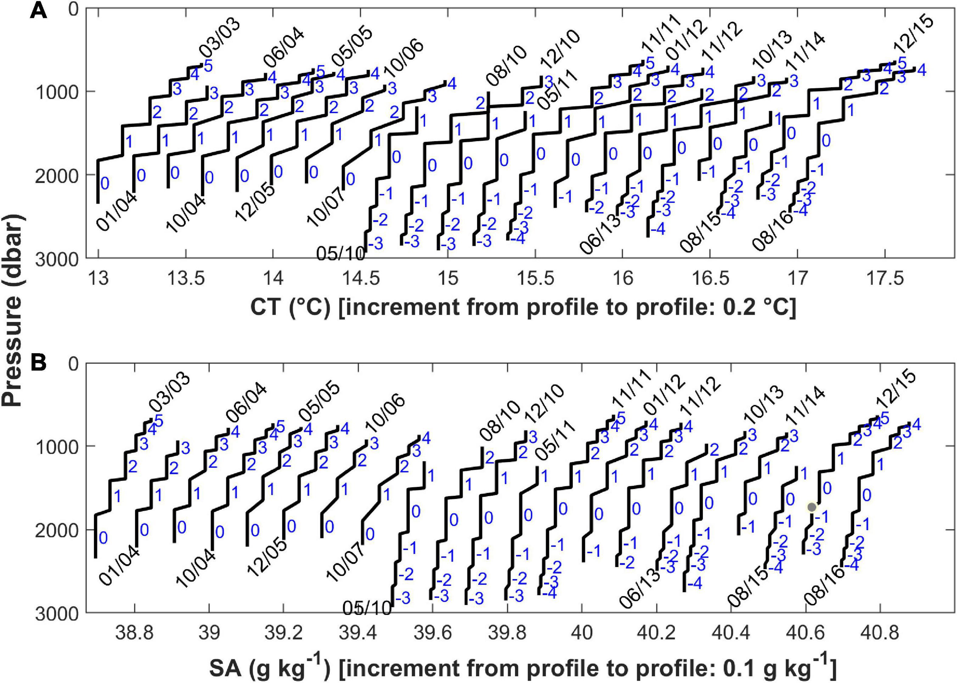
Figure 4. (A) CT (°C) and (B) SA (g kg^–1) profiles for each cruise obtained by matching the depth level of every detected corner point with the average value of CT and SA in the layer above (for a j_u corner point) or below (for a j_l corner point) it. Profiles are offset by 0.2°C and 0.1 g kg^–1 from cruise to cruise for better viewing. The layers are numbered as in Figure 3.

Calculation of Heat and Salt Fluxes

The local heat and salt fluxes, F_T and F_S – i.e., the heat and salt fluxes at the observed interfaces – were calculated using the H88 formulation of the Kunze (1987) model for thick interfaces, the RS12 model that accounts for secondary instabilities of salt fingers and the MP21 model which was developed for an inhomogeneous background stratification. In the formulations of the fluxes that follow, we consider the vertical (z) axis positive downward.

The H88 equations are:

$$\{\begin{array}{c}\hfill F_S=2\mathrm{\nu }⟨\frac{\partial S}{\partial z}⟩{\left(\sqrt{R_{\mathrm{\rho }}}+\sqrt{R_{\mathrm{\rho }}-1}\right)}^2\hfill \\ \hfill F_T=\mathrm{\gamma }\frac{\mathrm{\beta }}{\mathrm{\alpha }}{F}_S\hfill \\ \hfill \mathrm{\gamma }=\sqrt{R_{\mathrm{\rho }}}\left(\sqrt{R_{\mathrm{\rho }}}-\sqrt{R_{\mathrm{\rho }}-1}\right)\hfill \end{array}(3)$$

where v is the molecular viscosity of seawater, and $⟨\frac{\partial S}{\partial z}⟩$ is the salinity gradient in the interface. $R_{\mathrm{\rho }}=\frac{\mathrm{\alpha }\left(\frac{\partial T}{\partial z}\right)}{\mathrm{\beta }\left(\frac{\partial S}{\partial z}\right)}$ is the density ratio (Turner, 1973), $\mathrm{\gamma }=\frac{\mathrm{\alpha }{F}_T}{\mathrm{\beta }{F}_S}$ is the flux ratio (Kunze, 1987), and α and β are the thermal expansion and haline contraction coefficients for seawater.

These flux laws are valid for interfaces thicker than 30 cm and represent the maximum temperature and salinity fluxes due to salt fingers observed there. Therefore, they are also suitable for our staircase system where the interfaces are several tens of meters thick.

Equations (4.1) of Radko and Smith (2012), which provide non-dimensional fluxes, were transmuted into the dimensional domain by considering equations (2.3) of the same paper. The operation furnishes us with the dimensional eddy diffusivities of heat and salt as functions of the non-dimensional fluxes, F_T^∗ and F_S^∗, which we then multiply by the respective vertical gradients of CT and SA (Fick’s diffusion model). So, the dimensional fluxes can be written as follows:

$$\{\begin{array}{c}{F}_S=K_S⟨\frac{\mathrm{△}S}{\mathrm{△}z}⟩=k_T{R}_{\mathrm{\rho }}\left(\frac{a}{\sqrt{R_{\mathrm{\rho }}-1}}+b\right)⟨\frac{\partial S}{\partial z}⟩,(a,b)=(135.7,-62.75)\hfill \\ F_T=K_T⟨\frac{\mathrm{△}T}{\mathrm{△}z}⟩=k_T\mathrm{\gamma }\left(\frac{a}{\sqrt{R_{\mathrm{\rho }}-1}}+b\right)⟨\frac{\partial T}{\partial z}⟩\hfill \\ \mathrm{\gamma }=a_{\mathrm{\gamma }}exp\left(-b_{\mathrm{\gamma }}{R}_{\mathrm{\rho }}\right)+c_{\mathrm{\gamma }},(a_{\mathrm{\gamma }},b_{\mathrm{\gamma }},c_{\mathrm{\gamma }})=(2.709,\mathrm{\hspace{0.25em}2.513},\mathrm{\hspace{0.25em}0.5128})\hfill \end{array}(4)$$

where k_T = 1.4 × 10^–7 m² s^–1 is the molecular diffusivity of heat, and K_T and K_S are the dimensional eddy diffusivities of heat and salt, respectively.

Ma and Peltier (2021) gave functional forms for the flux ratio and the eddy diffusivities [their equation (1)]. The latter were used to derive the parameterizations of heat and salt fluxes as above, obtaining:

$$\{\begin{array}{c}{F}_S=K_S⟨\frac{\mathrm{△}S}{\mathrm{△}z}⟩=\frac{k_T{R}_{\mathrm{\rho }}}{\mathrm{\gamma }}\frac{a}{{(R_{\mathrm{\rho }}-1)}^b{R}_{\mathrm{\rho }}^c}⟨\frac{\partial S}{\partial z}⟩,(a,b,c)=(78.09,\mathrm{\hspace{0.25em}0.52},\mathrm{\hspace{0.25em}0.87})\hfill \\ F_T=K_T⟨\frac{\mathrm{△}T}{\mathrm{△}z}⟩=k_T\frac{a}{{(R_{\mathrm{\rho }}-1)}^b{R}_{\mathrm{\rho }}^c}⟨\frac{\partial T}{\partial z}⟩\hfill \\ \mathrm{\gamma }=a_{\mathrm{\gamma }}{R}_{\mathrm{\rho }}^3+b_{\mathrm{\gamma }}{R}_{\mathrm{\rho }}^2+c_{\mathrm{\gamma }}{R}_{\mathrm{\rho }}+d_{\mathrm{\gamma }},\hfill \\ (a_{\mathrm{\gamma }},b_{\mathrm{\gamma }},c_{\mathrm{\gamma }},d_{\mathrm{\gamma }})=(-0.00068,\mathrm{\hspace{0.25em}0.0163},-0.125,\mathrm{\hspace{0.25em}0.77})\hfill \end{array}(5)$$

For the calculation, the differential terms $(⟨\frac{\partial S}{\partial z}⟩,⟨\frac{\partial T}{\partial z}⟩)$ in equations (3), (4), and (5) have been discretized and approximated with $(\frac{\mathrm{△}SA}{\mathrm{△}z},\frac{\mathrm{△}CT}{\mathrm{△}z})$ (henceforth termed as SA_z and CT_z), where ΔSA (ΔCT) is the difference between the mean value of SA (CT) in the layers above and below an interface (i.e., the mixed layers of the surrogate profiles of Figure 4) and Δz is the thickness of the interface itself in meters. α, β and R_ρ were calculated with the TEOS-10 software (McDougall and Barker, 2011) for the pressure level associated with the point demarcating the interface using the temperature (CT) and salinity (SA) values of the adjacent layer. The routine that calculated R_ρ also generated a value for the Turner angle (Tu) because of the relation R_ρ = − tan (Tu + 45deg) (Ruddick, 1983) linking the two parameters. The molecular viscosity, ν, was calculated for all the surrogate profiles using the Seawater Thermophysical Properties Library (Sharqawy et al., 2010; Nayar et al., 2016), and a representative average value of 1.24 × 10^–6 m² s^–1 was derived from the obtained values.

We have estimated the contributions of the heat and salt fluxes, F_T and F_S, to the local buoyancy as gαF_T and gβF_S, where g is gravitational acceleration (9.8 m² s^–1). Then, the net buoyancy flux was quantified as the difference between these two buoyancy constituents: F_b = g (βF_s−αF_t). The salt finger instability produces vertical fluxes diffusing heat and salt down along their mean gradients. However, the vertical transport of salt is more efficient than that of heat. Consequently, the haline component of the buoyancy flux exceeds its thermal equivalent, resulting in an up-gradient flux of density (Turner, 1967; St. Laurent and Schmitt, 1999).

The flux calculations with the three methods are compared in Figure 5, which also shows the mean salt and heat fluxes and the flux ratio estimated by Ferron et al. (2021) from microstructure observations in the same area in the period 2013–2015. Although they use different functional relationships, RS12 and MP21 produced values for the salt and heat fluxes that are quite similar, with only very small differences in the case of heat (Figures 5A,B). These values are higher than those obtained for the same fluxes with H88 by a factor of 5 and 6 for heat and salt, respectively. The discrepancies are due to the differences in the underlying assumptions and parameterizations. Those between H88 and R12 have already been reported by Bryden et al. (2014) and Falco et al. (2016), and arise from the distinctive parameterizations with respect to R_ρ and on the specific constants used. This is immediately evident from Figure 5D, where the dependency of the salt flux on the density ratio in the three models is presented. The parameterizations of RS12 and MP21 provide values which decrease with R_ρ while that of H88 does the opposite. Disparities are also found in the dependence of the salt flux on the salinity gradient (not shown), which are due exclusively to the use of different constants in the models: numerically, the molecular viscosity in equations (3) and the molecular diffusivity of heat in equations (4) and (5), diverge from each other by an order of magnitude.

FIGURE 5

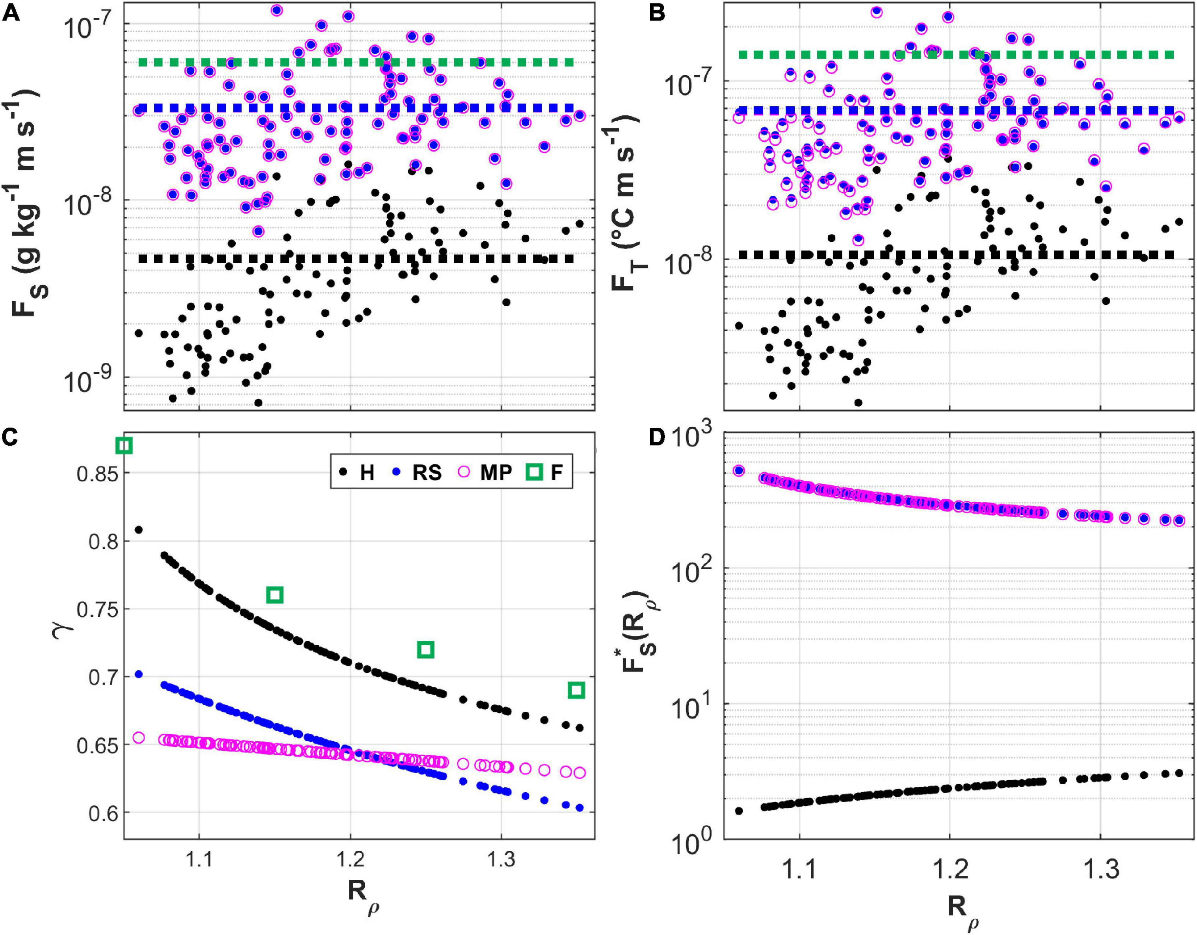
Figure 5. (A–C) Comparison of the calculations of salt flux, heat flux, and flux ratio with different methods (H = H88; RS = RS12; MP = MP21; F = Ferron et al., 2021). (D) The relationship between salt fluxes and R_ρ; F_S^∗(R_ρ) denotes the part dependent on R_ρ in equations (3)–(5). In (A) and (B), the dashed lines represent mean values calculated for the period 2013–2014 in the 600–2800 m depth range, and the axes expressing the fluxes are set to the logarithmic scale.

The comparison of the mean salt and heat fluxes obtained by Ferron et al. (2021) (green dashed line in Figures 5A,B) with those calculated by us from our dataset for the same period and depth range (blue and black dashed lines) as them showed that their computational scheme is much closer to RS12 and MP21 than to H88. The flux ratio values we obtained with our data (Figure 5C) are arranged exactly along the theoretical curves imposed by the equations (3), (4), and (5), i.e., γ^RS = f (e^−R_ρ), ${\mathrm{\gamma }}^{MP}=f\left(R_{\mathrm{\rho }}^3\right)$, and γ^H = f (R_ρ). They are close to 0.7, as could be expected in a salt finger regime (Schmitt, 1979), but are slightly lower in the RS12 and MP21 parameterizations than in H88. The H88 results for the flux ratio are more consistent with the values derived for the parameter from the microstructure observations. The flux ratio parameterization of MP21 varies only slightly when compared to those of both RS12 and H88 in our density ratio range. Overall, however, they resemble the fluxes coming from RS12 rather closely.

Results

Time Evolution of the Thermohaline Properties in the Measurement Period

Durante et al. (2019) have already shown that thermohaline properties change over time and along the water column, and relate these changes to the variations observed in the LIW. Here, we carry this study forward by analyzing how the salinity and temperature at the level of the LIW and in the underlying layers changed over the period covered by the observations, and examining the natures of the associated trends.

Figures 6A,B shows the maximum salinity value and corresponding temperature for each profile, which denote the LIW signal in our observational domain. Furthermore, it presents the average salinity and temperature in the layers labeled 0 and 1 in Figure 3 and in the deep layer. Layer 0 is the thickest layer in each profile (located within the gray area in Figure 3) and layer 1 lies just above it. Both layers are well-developed in all the profiles, and correspond to the main-middle pair of layers in Figure 4 of Durante et al. (2019). We have identified the deep layer as the part of the water column comprising the last 500 dbar above the bottom which is not affected by the formation of steps. However, the average values of the two parameters and associated trends do not change significantly even if we reduce its thickness to just 100 dbar from the bottom. We have not shown the standard deviations associated with the mean values in the figure because they are very small in all the layers, and are not appreciable on the plot scale.

FIGURE 6

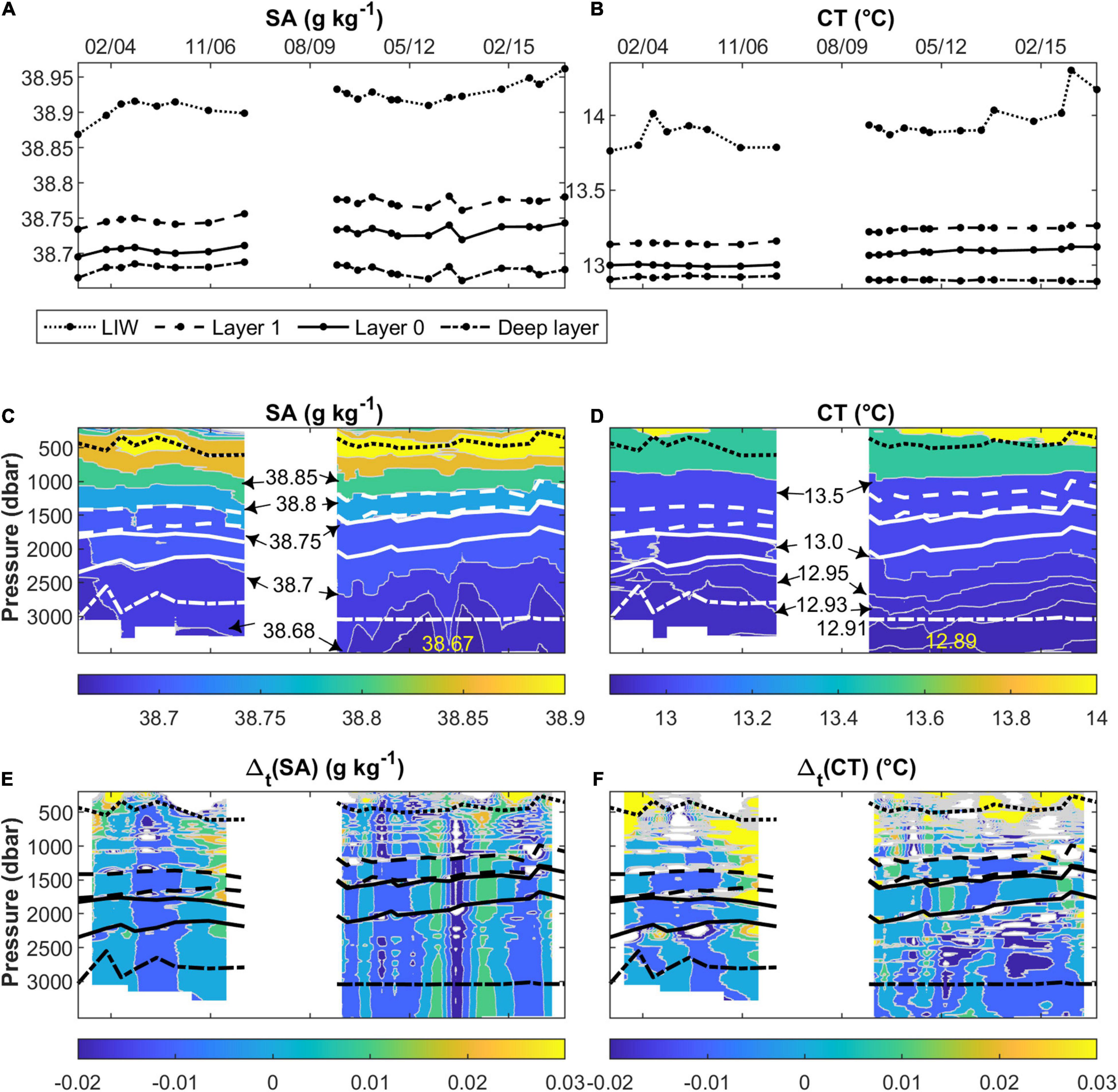
Figure 6. Evolution over time of salinity (SA) and temperature (CT). (A) and (B) show the variation of the maximum salinity and its corresponding temperature value (LIW), together with the average values of SA and CT in the layers 0 and 1 of the staircases, and in the last 500 dbar above the bottom. (C) and (D) present the behaviors of salinity and temperature with respect to pressure and time. (E) and (F) the same, only this time for the calculated difference in salinity and temperature between two consecutive times instead. In (C–F), the position of the LIW and the previously specified 0, 1 and deep layers are indicated using the types of lines ascribed to them in the legend of (A) and (B).

Trends of salinity and temperature are estimated as the slopes, accompanied by their standard errors, of a linear regression model. The LIW shows warming and salinification trends of 0.019 ± 0.005 °C yr^–1 and 0.0036 ± 0.0006 g kg^–1 yr^–1, in line with the values reported by Schroeder et al. (2017) for the same trends in the Strait of Sicily (0.024 °C yr^–1 and 0.006 yr^–1; the latter value does not change if expressed in g kg^–1 yr^–1). Our somewhat lower values can be attributed to the changes the LIW undergoes due to mixing with the waters it encounters during its journey from the Strait of Sicily to our measurement area (Millot and Taupier-Letage, 2005). Another possible reason for this slight diminution is the fact that the core of the LIW moves mainly along the boundaries of the Tyrrhenian Sea, so its signal in our area tends to be principally modulated by lateral advection (Astraldi and Gasparini, 1994; Zodiatis and Gasparini, 1996). The layers 0 and 1 also present warming and salinification trends, but they are slower compared to those of the LIW. The temperature varies at a rate of 0.011 ± 0.001 °C yr^–1 in both layers, and the salinity by 0.0031 ± 0.0004 g kg^–1 yr^–1 in layer 1 and 0.0032 ± 0.0004 g kg^–1 yr^–1 in layer 0. In the case of the deep layer, the variations of the two properties are very small and their trends are contrary to those characterizing the water column above (−0.0023 ± 0.0004 °C yr^–1 and −0.0005 ± 0.0004 g kg^–1 yr^–1). The trends of the deep layer coincide with the intrusion of less salty (<38.68 g kg^–1) and colder (<12.93°C) water (Figures 6C,D) coming from the Western Mediterranean (Schroeder et al., 2016). This intrusion is present from December 2010 to December 2015. It is not persistent and is more visible in salinity than in temperature. It is not observed in May 2011, June 2013, November 2014, and August 2015, which correspond to periods when the 38.68 g kg^–1 isoline sinks toward the bottom, as can be seen in Figure 6C. In January and November 2012, and in October 2013, the lowest salinity value of the whole dataset, equalling 38.66 g kg^–1, is observed below 3250 dbar. The detected intrusion seems to be causing the isolines of both salinity and temperature to rise. The layers 0 and 1 behave likewise, with an upward displacement. Figure 3 shows that the entire staircase system is subjected to this uplifting. The deep layer appears isolated from those above it and does not seem to benefit at all from the possible heat and salt inputs driven downward by the salt fingering phenomenon.

The differences noted in salinity and temperature at the same pressure level at two consecutive times (Figures 6E,F) suggest that our profiles are contaminated by internal waves (see Figure 1d in van Haren and Gostiaux, 2012, for a possible corroboration). Over time, such differences swing back and forth between positive and negative values in extended portions of the water column, suggesting that they are caused by low salinity, low temperature or high salinity, high temperature water types being pushed up and down by wave motion. This pattern is complicated by cases in which the layer is squeezed from above and below due to the probable passage of out-of-phase waves, which mainly occurs in the period 2003–2007. Internal gravity waves occupy a frequency range bounded by the local inertial frequency below and by the Brunt-Väisälä frequency above (Garrett and Munk, 1975). In the Tyrrhenian Sea, where our observations were made, the local inertial period is 18.7 h. This is an upper limit for the sampling time needed to resolve internal waves. Our coarse sampling interval does not allow us to resolve the frequencies of internal waves, and therefore to investigate how they interact with the staircases. In deep water and far from topography, as in our case, the contribution of such waves to the vertical mixing could be relevant (Munk and Wunsch, 1998).

Staircase Properties

The staircase system consists of a series of main layers (thicker than 90 dbar) with several thinner layers above and, from 2010, below, which are separated by interfaces showing a rich variety of structures. Durante et al. (2019, their Table 1) classified the interfaces into four classes: sharp, slope, steppy, and rough. Sharp interfaces present relatively large gradients of temperature and salinity in a short vertical interval (what we expect for a theoretical staircase in equilibrium), such as those observed above 1500 dbar in Figure 3 in March 2003 and April 2004. Slope interfaces are like sharp interfaces, but thicker (the gradients are more extensive vertically). They are common at the base of a staircase (seen, for example, from May 2010 onward in the same figure), but are also found at intermediate depths (as noticeable between layers 1 and 2 in June and October 2004, again in Figure 3). Steppy interfaces, like those evident between layers 1 and 2 in October 2013 and November 2014, incorporate small layers which may or may not be homogeneous (i.e., they might have small gradients from top to bottom or in the middle) with additional interfaces between them. Rough is a further attribute which characterizes some of the slope and steppy interfaces that show certain kinds of irregularities. To simplify, we will consider only the three main types of interfaces, i.e., sharp, slope and steppy, regardless of their roughness, in this section.

The layers can vary in number from one profile to another, and their level of development may also differ. They are more abundant in the period 2010–2016 than in the period 2003–2007. The thickest layer in each profile (layer 0, in Figure 3) migrates upward from 2010 onward when more layers can be distinguished below it. The thickness of each layer varies over time. For example, the thickness of layer 0 is 510 m in March 2003, 280 m in October 2007, 502 m in May 2010, and 380 m in August 2016.

The prevailing patterns of stratification are reflected in the distributions of the values of the Turner angle associated with the layers and the interfaces, as shown in Figure 7. The figure presents histograms depicting the density of observations relating to the layers and the interfaces obtained from the untreated and the low-pass filtered data with a vertical resolution of 1 dbar in different bins of the local Turner angle. The dominant stratification within the layers is of the stable type (−45 < Tu < 45 deg), embracing 83% and 95% of the observations in the original and filtered profiles, respectively. Other configurations are also present, including the gravitationally unstable type, but to a smaller extent, so they are largely removed by the filter. Similarly, within the interfaces, various configurations are observed, with stable and finger (45 < Tu < 90 deg) types prevailing. There are interfaces that include gravitationally unstable zones (Tu > 90 deg), too. In terms of the fraction of observations they represent, the three mentioned interface configurations are distributed thus in the untouched and filtered sets of profiles, respectively - stable: 36%, and 16%; finger: 36%, and 54%; gravitationally unstable: 26%, and 30%. Filtering the original profiles brings out the finger instability type as the prevalent configuration. It is worth noting that even in the filtered profiles there remain areas within the interfaces that are gravitationally unstable.

FIGURE 7

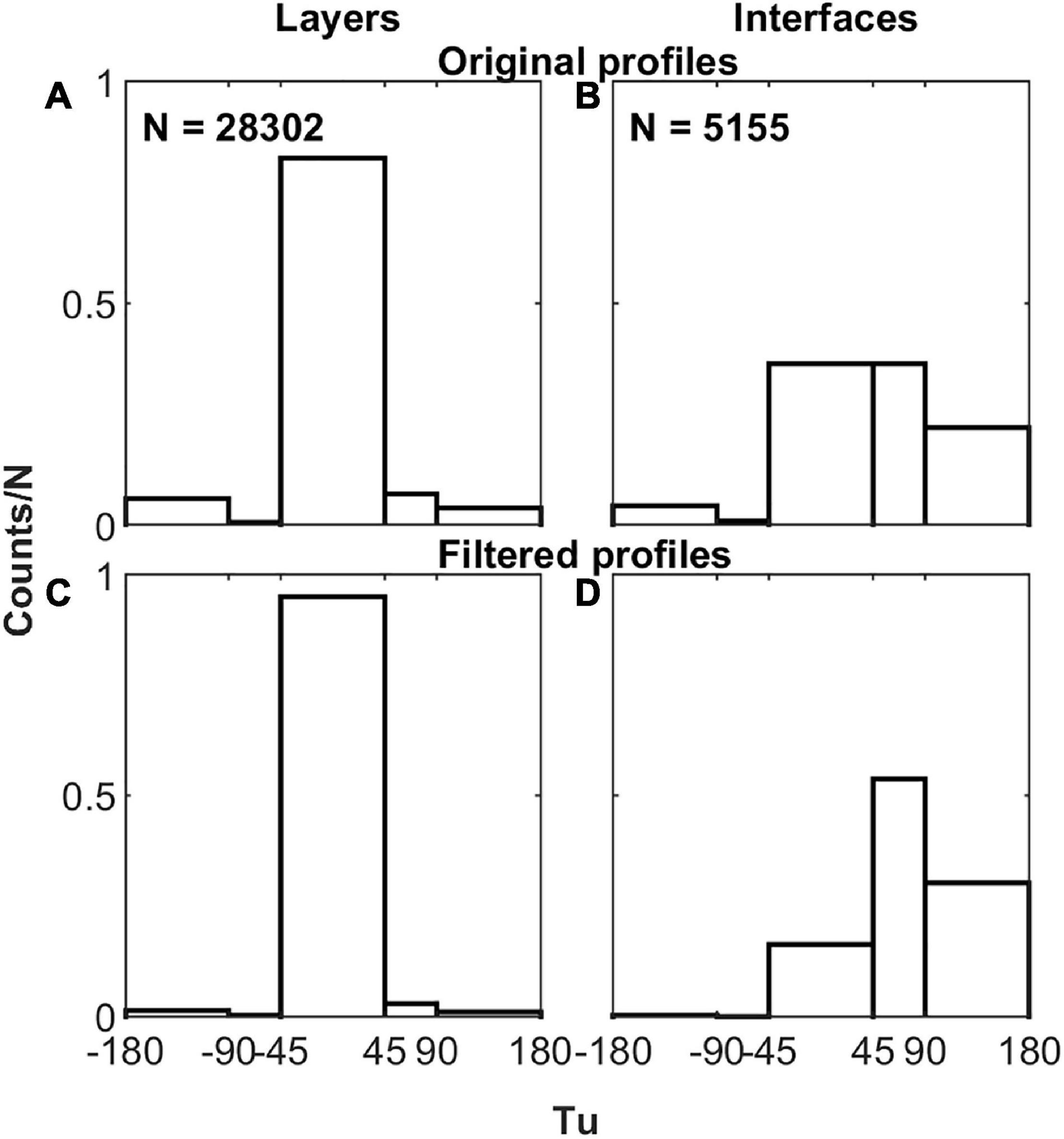
Figure 7. (A,C) Histograms categorizing the density of observations in the layers extracted from the original and filtered profiles on the basis of the Turner angle. (B,D) The same, only this time for the interfaces instead of the layers.

To identify the main features of the typical staircase, we used the surrogate profiles of Figure 4. Note that the perturbations within layers and interfaces are therefore not considered. The thickness of the layers, h_l, ranges from 60 to 510 m (Figure 8A), and shows a tendency to increase linearly with depth down to about 1850 dbar. At greater depths, h_l decreases. As for the interfaces, their thickness, h_i, is very variable, ranging from 15 m to several hundreds of meters (Figure 8B). The thickest interfaces are those of the slope and steppy types. The sharp interfaces have, at most, thicknesses of 44 m. Figure 8C presents the ratios between the thicknesses of the interfaces and their underlying layers. We noticed that sharp interfaces are never more than quarter the size of their underlying layers. On the contrary, the other two types of interfaces can reach sizes of up to 40% of the extensions of the layers below them, and sometimes even more. According to Zhurbas and Ozmidov (1984), the ratio between the thicknesses of the interfaces and the underlying layers may vary depending on the process that generated the step they are part of. In particular, from theoretical reasoning and some considerations on the geometric properties of a profile containing steps, they derived qualitative reference limits for this ratio in the presence of different generation mechanisms. They suggested that the characteristic range for double diffusion should be $0.02\le \frac{h_i}{h_l}\le 0.25$. Higher values would indicate the dominance of other processes such as the kinematic effect of internal waves (∼1) and the local effects of turbulent mixing (intermediate values, between 0.25 and 1). Unfortunately, we are unable to quantify the possible effects of similar processes on the Tyrrhenian staircases as this would require additional data which we do not have. However, in the case of slope interfaces, which often also show roughness, it is very likely that there are other processes in action besides double diffusion. In the case of steppy interfaces, a separate discussion should be made, going into the details of their substructure and evaluating the ratio between each sub-interface and sub-layer. The values we report for the ratio in Figure 8C are certainly overestimated for steppy interfaces, because we have established their thicknesses for the calculations by considering them in their entirety, i.e., from the top to the bottom.

FIGURE 8

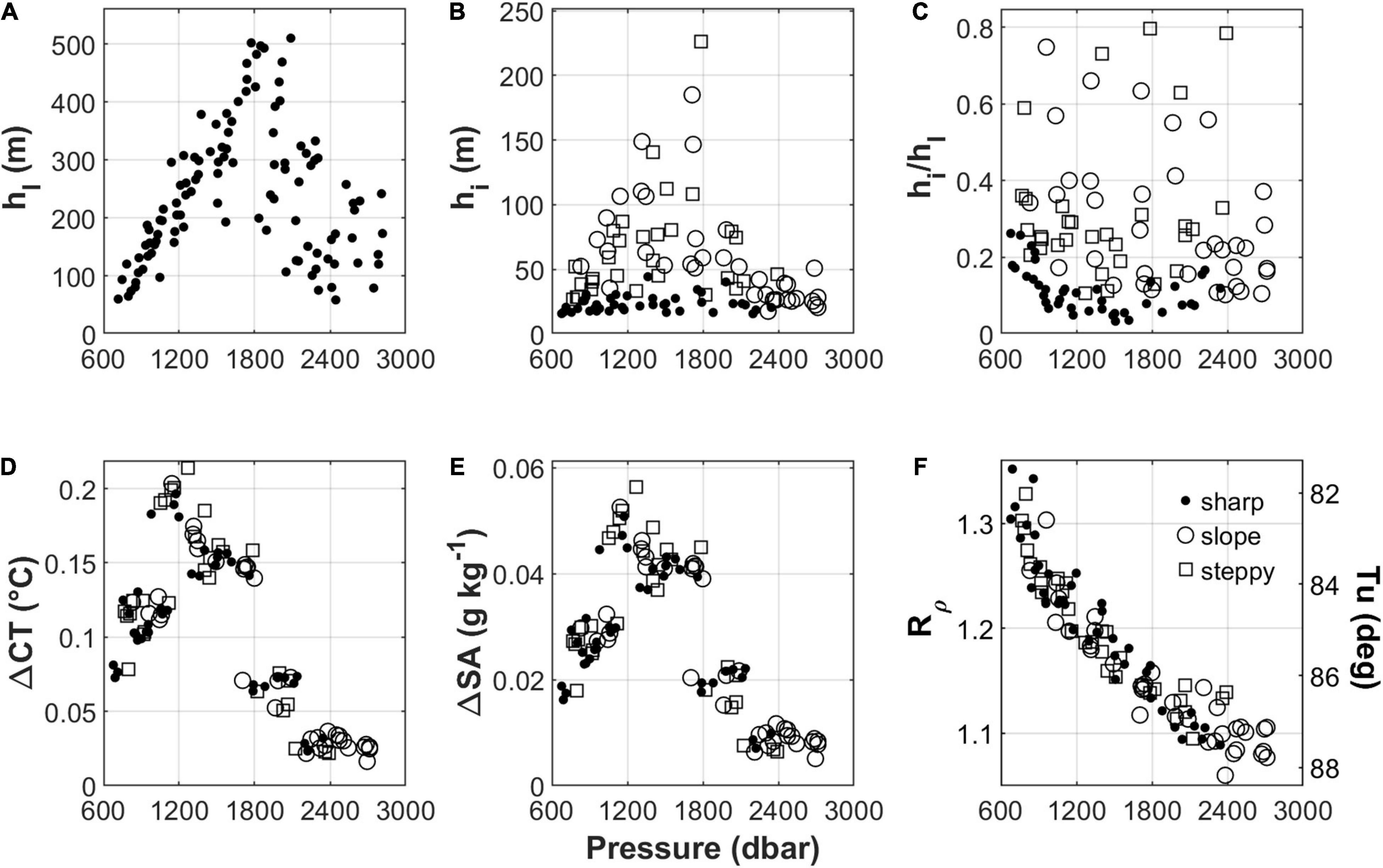
Figure 8. Main features of the staircase system vs. pressure (dbar). (A) Layer thickness (m), referring to the midpoint of the layer. (B) Interface thickness (m), referring to the midpoint of the interface. (C) Ratio between the thickness of the interface and the underlying layer. (D,E) Differences of the temperature (°C) and the salinity (g kg^–1) across an interface. (F) Density ratio (left axis) and the correspondent values of the Turner angle (right axis). In (B–F), the values corresponding to the different types of interfaces (sharp, slope, steppy) are denoted by the symbols ascribed to them in the legend of (F).

The differences in temperature and salinity across the interfaces, ΔCT and ΔSA, corresponding to the disparities between the layer above and below the interface in the two properties, vary in the range 0.02–0.2 °C and 0.005–0.06 g kg^–1, respectively (Figures 8D,E). The greatest variations are observed in the pressure range 980–1800 dbar, regardless of the type of interface.

The values obtained for the density ratio R_ρ and the Turner angle Tu (Figure 8F), falling as they do in the limits 71.6 < Tu < 90deg and 1 < R_ρ < 2 describing a fingering regime (Ruddick, 1983), confirm the ubiquitousness of the phenomenon in the area. R_ρ (Tu) decreases (increases) from the top to the bottom, where it tends to approach unity, and is always less than 1.7. This is usually associated with the appearance of step-like structures in vertical T-S profiles (Schmitt, 1981; Schmitt et al., 1987; Radko et al., 2014a). The lowest values of R_ρ are associated with slope interfaces, which are frequently found at the bases of the staircases.

Heat and Salt Fluxes Through Interfaces

Local fluxes vary both with depth (pressure) and in time. We began by examining the variabilities of the salt and heat contributions to the buoyancy, namely gβF_S and gαF_T, and their difference, the net buoyancy flux F_b, with the pressure p and the density ratio, R_ρ. Plots of gβF_S, gαF_T, and F_b with respect to p (Figures 9A,C,E) and R_ρ (Figures 9B,D,F) almost mirror each other, reflecting the R_ρ (p) relationship already evidenced in Figure 8F. As already noted, the fluxes obtained with RS12 are higher than those calculated with H88, but the trends of the estimates as a function of the pressure and of the density ratio are almost the same in both the cases. The values are generally larger in the portion of the water column between 600 and 1800 dbar where R_ρ> 1.15, mainly in correspondence with sharp interfaces. Below 1800 dbar, they start to decrease, reaching minima at the bottoms of the staircases, typically in the presence of slope interfaces. To provide a sort of reference “frame” for broadly characterizing the portion of the water column affected by the staircase phenomenon at the studied location in terms of the fluxes, we have used our results to estimate some basic statistics for them in different pressure ranges, as reported in Table 1. The decrease in the fluxes with depth is greater in the results obtained with H88. The average net buoyancy flux obtained from the RS12 parameterization is (0.8 ± 0.6) × 10^–10 W kg^–1 – close to the value of (1.2 ± 4%) × 10^–10 W kg^–1 obtained by Ferron et al. (2021) for it in the same region, and by Bryden et al. (2014) for the staircase in the Algerian basin (1 × 10^–10 W kg^–1) – while that from H88 is about an order of magnitude lower, approximately (0.10 ± 0.08) × 10^–10 W kg^–1.

FIGURE 9

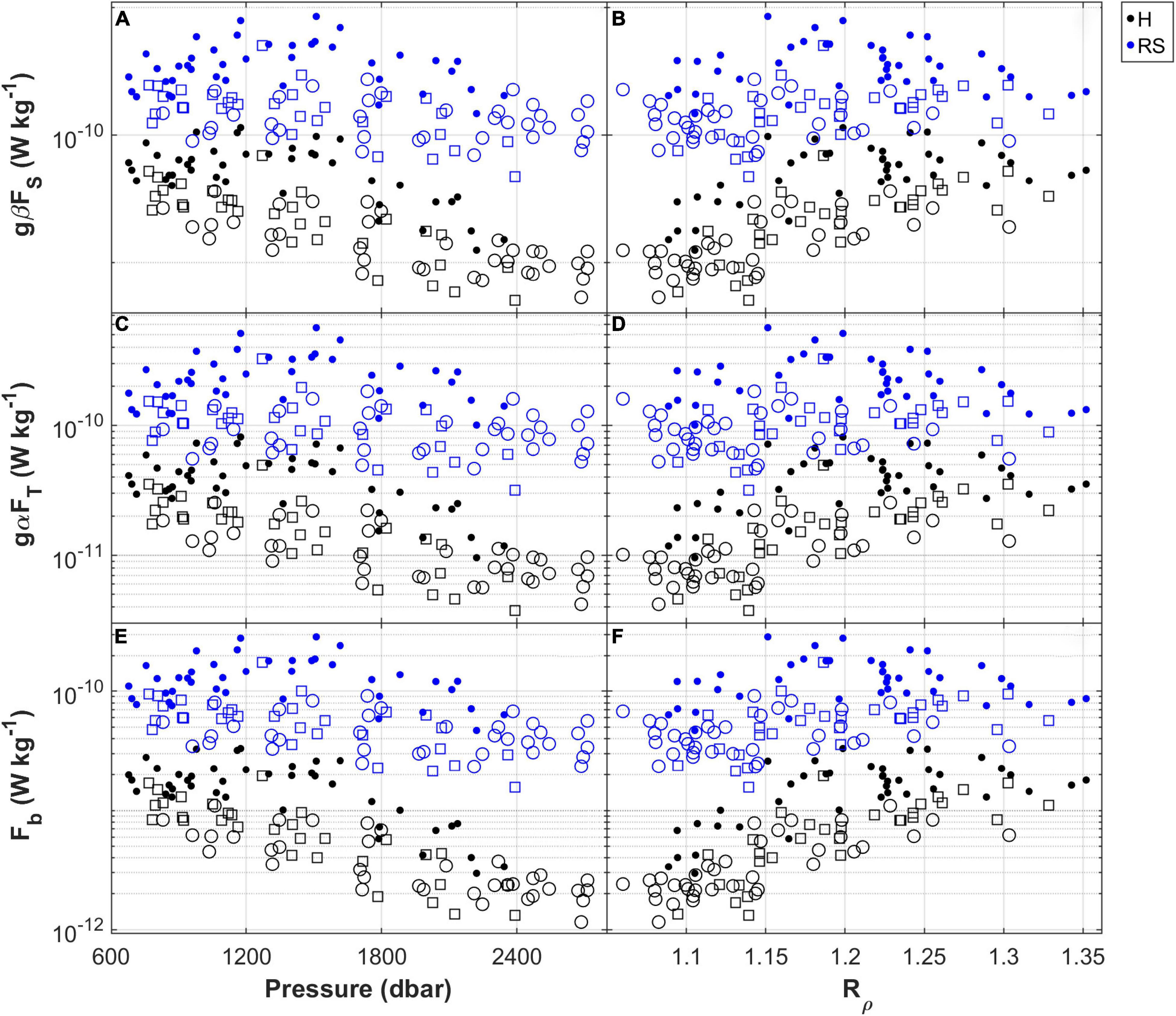
Figure 9. (A,C,E) The salt and heat contributions (gβF_S and gαF_T) to the buoyancy flux and the net buoyancy flux (F_b) versus pressure. (B,D,F) The same, but this time versus the density ratio (R_ρ) instead of pressure. Sharp, slope and steppy interfaces are represented by a black circle, a white circle and a white square, respectively. In the legend, H and RS refer to H88 and RS12, respectively. The axes expressing the fluxes are set to the logarithmic scale.

TABLE 1

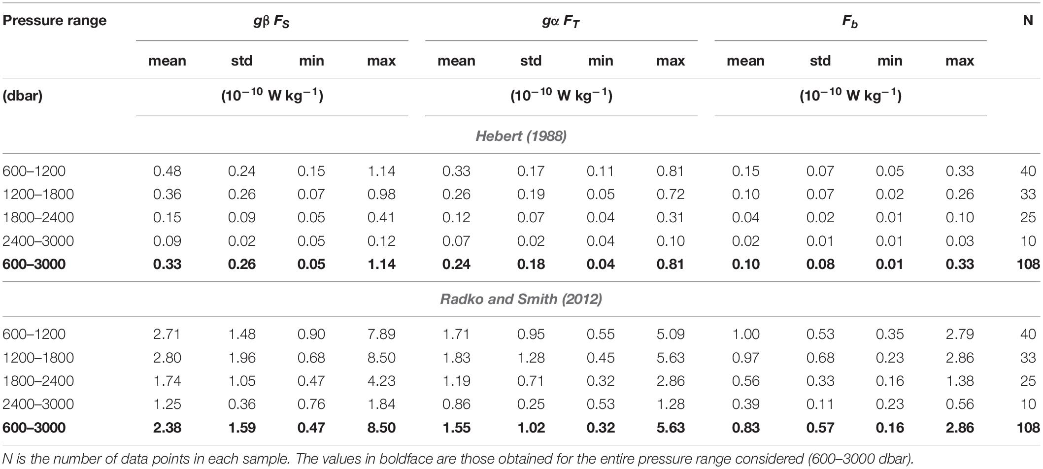
Table 1. Some basic statistics (mean, standard deviation, minimum, and maximum) summarizing the fluxes calculated in different pressure ranges with the two models, H88 and RS12.

The ratio between heat (salt) fluxes and the vertical gradients of temperature (salinity) provides an estimate of the eddy diffusivities of heat (salt). Figure 10 shows the relationships of the heat and salt fluxes, F_T and F_S, with their respective gradients, CT_z and SA_z. The two datasets are aligned along straight lines whose slopes can be considered representative of the eddy diffusivities in our salt finger region: K_S = (6.2 ± 0.1) × 10^–6 m² s^–1 and K_T = (3.56 ± 0.02) × 10^–6 m² s^–1 with H88, and K_S = (3.80 ± 0.09) × 10^–5 m² s^–1 and K_T = (1.92 ± 0.07) × 10^–5 m² s^–1 with RS12.

FIGURE 10

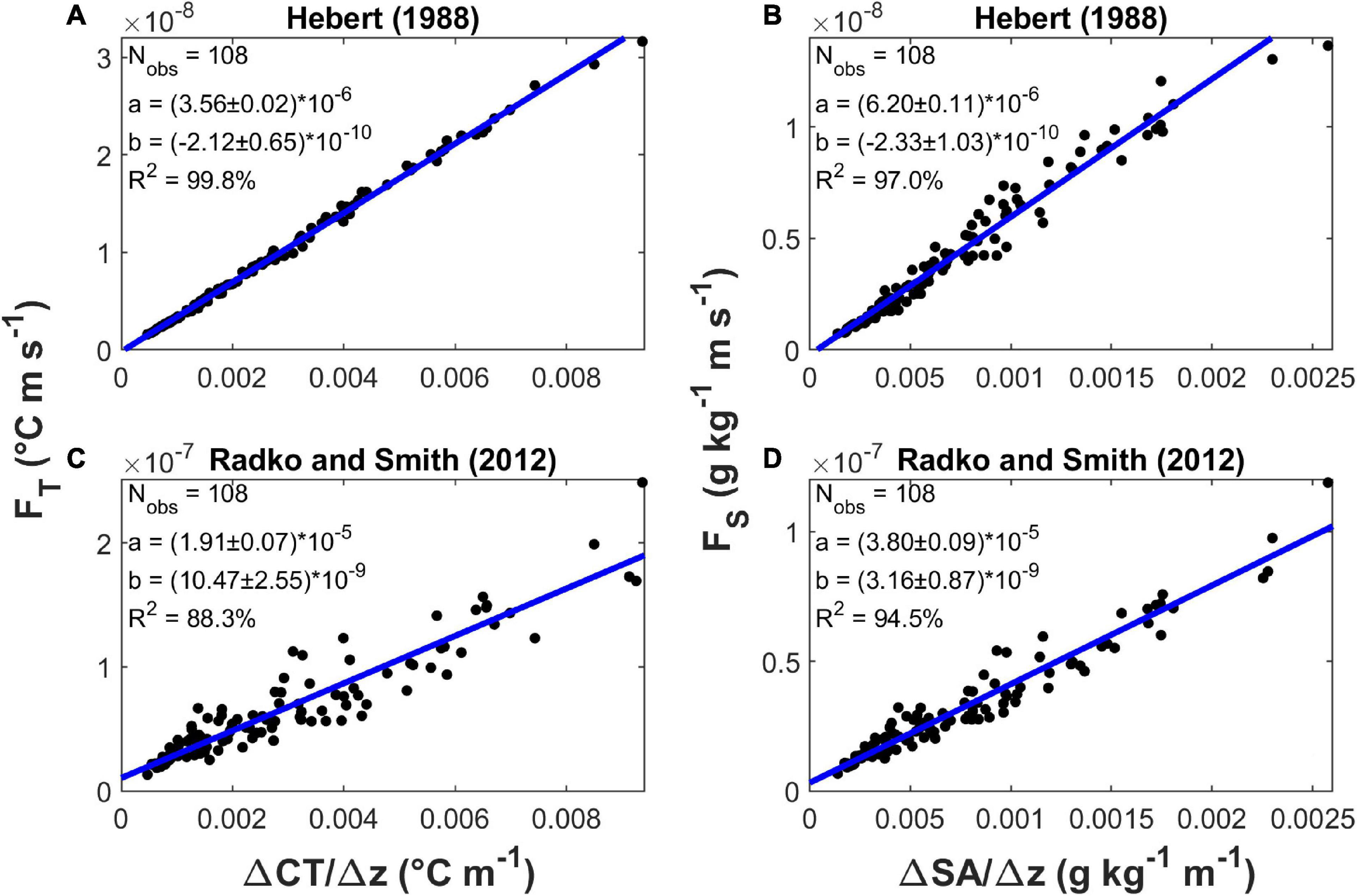
Figure 10. Fluxes versus gradients. (A) Heat flux F_T (°C m s^–1) versus CT gradient (°C m^–1), with H88. (B) Salinity flux F_S (g kg^–1 m s^–1) versus SA gradient (g kg^–1 m s^–1), with H88. (C) Heat flux F_T (°C m s^–1) versus CT gradient (°C m^–1), with RS12. (D) Salinity flux F_S (g kg^–1 m s^–1) versus SA gradient (g kg^–1 m s^–1), with RS12. Each panel includes the slope (a) and the intercept (b) of a linear fit (Matlab function fitlm) to presented data, accompanied by their standard errors; a value for R² is also reported.

Time series of local heat and salt contributions to the buoyancy flux calculated with RS12 are shown in Figure 11 (the equivalent resulting from the application of H88 is provided as Supplementary Figure 1). Comparing the two periods 2003–2007 and 2010–2016, it can be seen that the fluxes in the first period are weaker than those in the second, even in the presence of sharp interfaces. Furthermore, in both the periods, there are situations where the fluxes are low along the entire water column. This happened from May 2005 to October 2007, in May 2011 and in June 2013, and corresponded with occasions when interfaces were rough and predominantly of the slope or steppy type. In May 2005, October 2006, and October 2007, the entire profile was rough (Table 1 in Durante et al., 2019). These profiles are squeezed from above and below, probably due to the passage of out-of-phase internal waves (as previously mentioned in Section “Time Evolution of the Thermohaline Properties in the Measurement Period”), considerably reducing their thicknesses. The profiles of January 2012 and August 2015 also show particularly low fluxes, but with interfaces which are steppy. We will evaluate this kind of situation better in the following section.

FIGURE 11

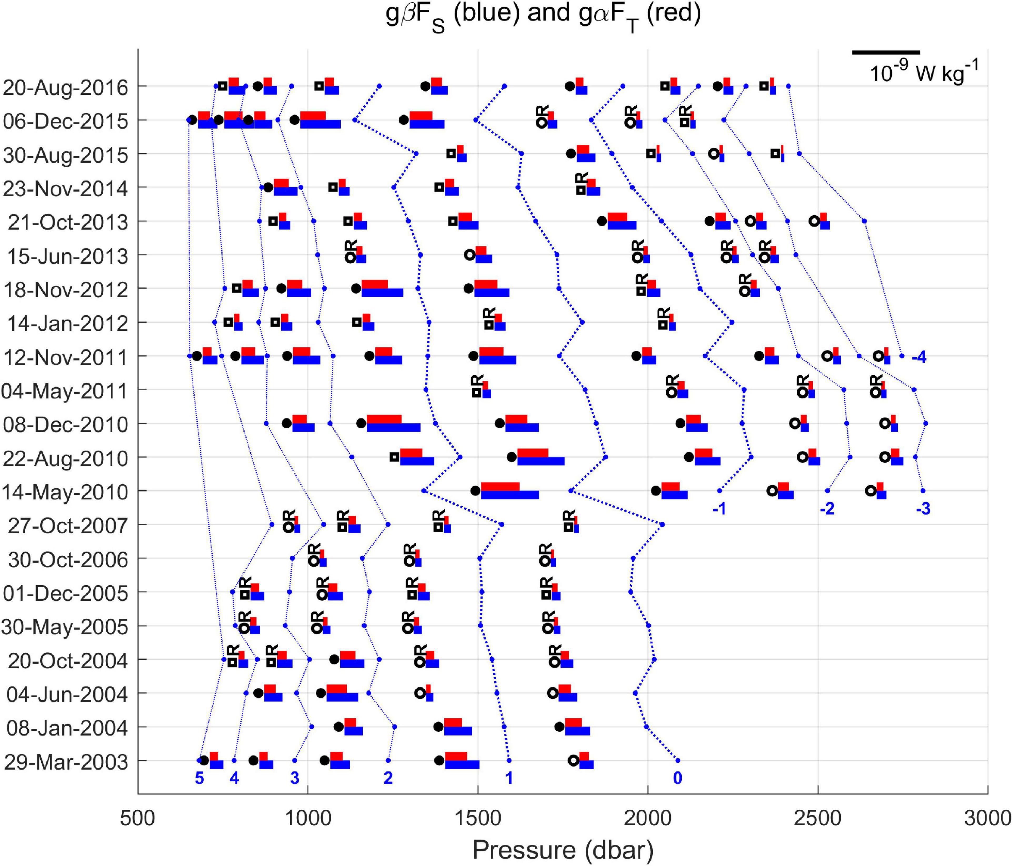
Figure 11. The heat and salt contributions (gαF_T and gβF_S) to the buoyancy flux over time, calculated with RS12. Each value is represented by a colored bar: blue for the salinity and red for the temperature. The scale is 10^–9 W kg^–1. Sharp, slope and steppy interfaces are represented by a black circle, a white circle and a white square, respectively. Rough interfaces are identified with the capital letter “R.” A layer is delineated by a blue line running through its middle.

Another point to underline is that the strongest fluxes seem to be occurring mainly between 700 and 1600 dbar, which confirms the process is much more intense below the lower limit of the LIW. The largest fluxes occur at the upper boundaries of layers 1 or 2 in the first period, and layers 0 or 1 in the second period. Furthermore, the portion of the water column affected by high fluxes moves upward, a consequence of the upward migration of the staircases. Vertical displacements of layers and interfaces have been ascribed to the action of internal waves (Johannessen and Lee, 1972; Schmitt et al., 1987). This would seem to explain the vertical displacements in the period 2003–2007, when the staircases showed both upward and downward movement. But since 2010, even though there is an up-and-down swing, a trend is also evident with all the major layers moving upward by several hundred meters. This coincides with the formation of additional layers below 2000 dbar. We think that the intrusion of nWMDW near the bottom plays a role here, both by pushing the old resident water upward and by causing new steps to be generated as a result of the enhancement of the necessary downward heat and salt fluxes. However, it should be emphasized that the fluxes through the interfaces that separate these supplementary layers are small: just 6–27% of the highest values (gαF_T = 5.63 × 10^–10 W kg^–1 and gβF_S = 8.50 × 10^–10 W kg^–1), obtained between layer 1 and layer 0 in May 2010.

Figure 12 shows the net fluxes of salinity and temperature in the layers situated between pairs of interfaces for which the fluxes were calculated (see Figure 11). The net flux in a layer is the upper interface flux minus the lower interface flux. A negative net flux means that the layer exports the property. A positive net flux means exactly the opposite. The last layer depicted in Figure 12 is the penultimate layer of the staircase identified in Figure 3. We cannot calculate the net fluxes in the first and last layers of the staircase because we do not know their ingoing and outgoing fluxes, respectively. There is a tendency of the staircase to gain salt and heat (positive net fluxes) in the layers located at intermediate and deep depth levels, while those above are more inclined to lose them. Net fluxes in layers 1 and 0 are predominantly positive and those in layer -1 (observed only from 2010 onward) are always positive. These are the thickest layers in the vertical sequence, layer 0 being the thickest of all, followed by the other two. At different times, at least one of these layers has net positive fluxes. The only exception is observed in June 2004, where we only have the net fluxes in layer 1, and they are negative; however, the layer 2 above has positive net fluxes of high magnitude, indicating it is the layer gaining salt.

FIGURE 12

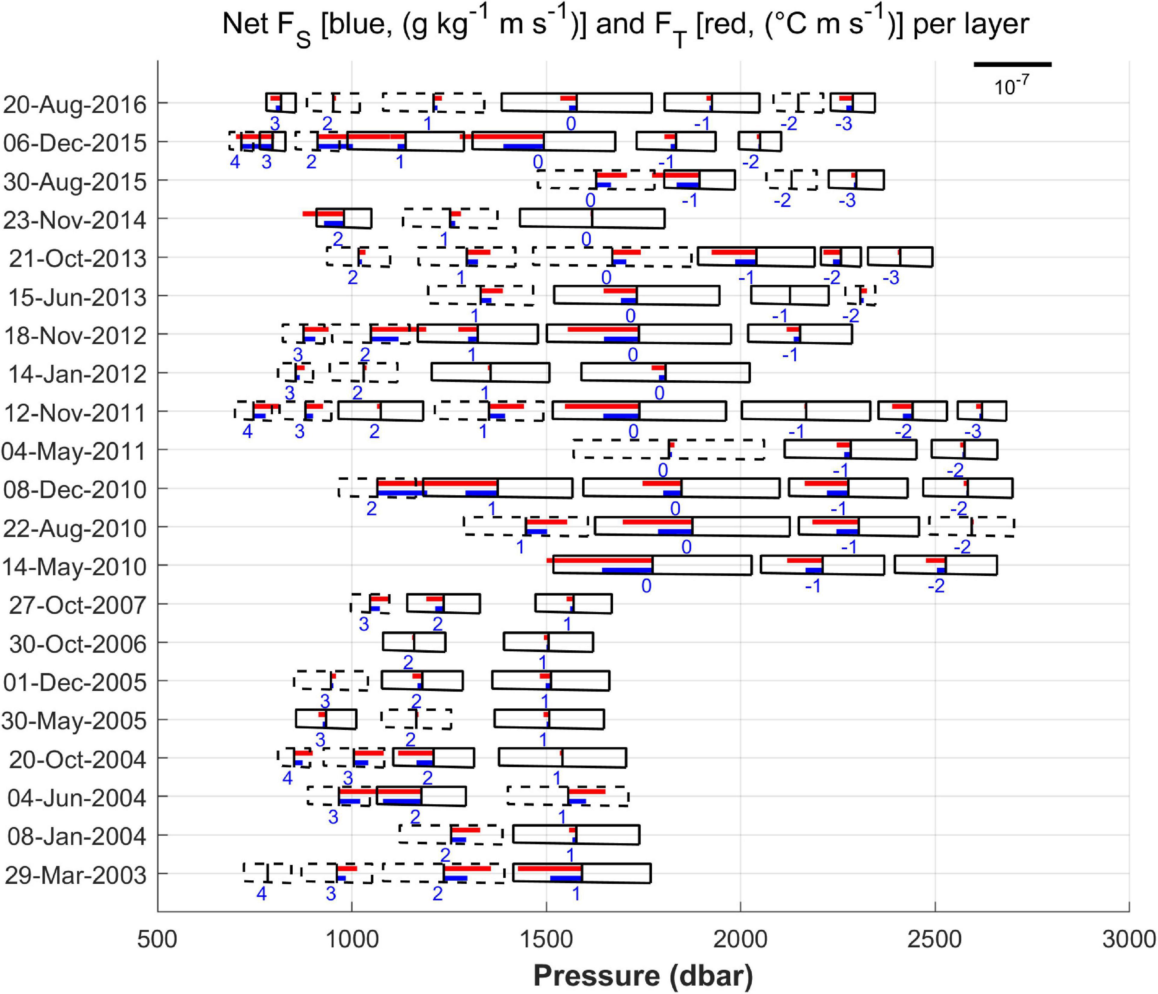
Figure 12. The net fluxes of salinity and temperature (RS12) associated with the layers, i.e., the upper interface flux minus the lower interface flux for each layer. The rectangles represent the layers, numbered following the scheme laid down in Figure 3. A dashed line delimiting a layer means that it exports more salinity/temperature than it receives, and a similar solid line means exactly the opposite. The orientation of a flux bar to the left or to the right indicates a net flux into or out of a layer, respectively.

Moving to the base of the staircase, we see that the penultimate layers have mainly positive net fluxes, with very few exceptions, so they also tend to gain salt and heat. This is in addition to the fact that from 2010 onward, the fluxes in the deeper interfaces are very small compared to those obtained for the central part of the staircases. This result might explain the trend reported in Section “Time Evolution of the Thermohaline Properties in the Measurement Period” for the deep layer, suggesting that it is generally isolated from what is happening above and does not benefit much from the heat and salt intake pushed downward by the salt fingering process.

Assessing the impact of net fluxes on the heat and salt content of a specific layer is challenging, and near to impossible, seeing that we do not know how long they are effective. However, just to give an idea, a positive net flux on the order of 10^–7 would raise the salinity (temperature) of 100 m of the water column by an amount equal to the trend calculated in section “Time evolution of the thermohaline properties in the measurement period” for layers 0 and 1 in about 1 month (4 months). Since the thicknesses of the two layers are greater than 100 m, it follows that the actual times would be longer. The reality is still more complicated. As shown in Figure 12, the net fluxes can even be two orders of magnitude lower, and layers can retain or release the relevant properties depending on the existing conditions. What is certain is that staircases play a significant role in the transfer of temperature and salt downward in the Tyrrhenian Sea, and therefore contribute in a noteworthy way to the diapycnal mixing in the area where they are found.

Fluxes in Interfaces With a Stepped Substructure

In the calculations presented in the previous section, we simplified the steppy interfaces as delimited by their uppermost and lowermost limits, ignoring any internal substructure. The approximation, while reasonable for the period 2003–2007 during which it is difficult to discern finer detail within such interfaces, is not always readily applicable later. This is particularly evident in the profiles corresponding to the interval extending from January 2012 to August 2016, which we examine below.

First, for each of the steppy interfaces shown in Figure 13A, we selected all the points identifiable visually in the original profiles as the ends of its sub-layers and sub-interfaces by hand. The original profiles were used because many of these substructures had been filtered out in their surrogates. Then, we recalculated the fluxes through the now more resolved interfaces and compared the results to those obtained by us for them in our previous calculations (Figures 13B,C).

FIGURE 13

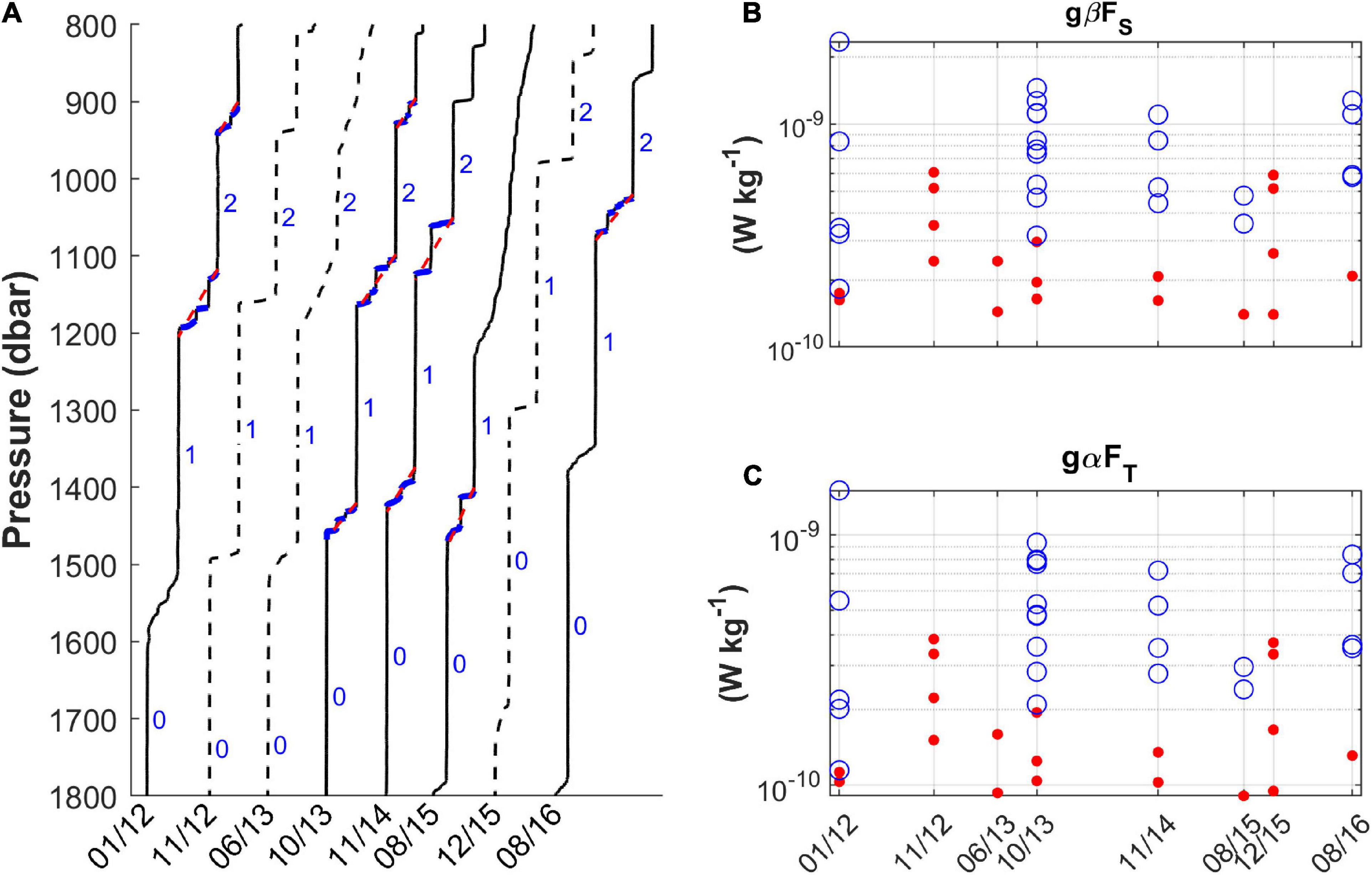
Figure 13. (A) Evolution of the Tyrrhenian staircases between 800 and 1800 dbar from January 2012 to August 2016. Steppy interfaces are delineated in blue. The dashed red lines represent their approximations, with the upper and lower limits demarcated. (B,C) Comparison of the estimated contributions of salt and heat to the buoyancy flux (RS12) for the steppy (blue circles) and rectified (solid red circles) interfaces. The axes expressing the fluxes are set to the logarithmic scale.

The number of homogeneous layers embedded in the steppy interfaces varies from one profile to another and with the depth, and so do their thicknesses which range from a few meters to some tens of meters. The largest sub-layers, 36, 54, and 35 m thick, are in the profiles of January 2012, November 2014 and December 2015. The shape of the interfaces changes from profile to profile too, taking on different forms, including sharp (in November 2012 and December 2015) and slope (in June 2013). Although there seems to be a continuity in the evolution of some substructures between consecutive profiles – for example, the large sub-layer of November 2014 which occupies the space previously occupied by the steppy interface of October 2013 that suggests a merging event of some kind – we cannot say with certainty if this is actually true. The long intervals of time between successive samplings strongly limit our ability to follow relevant step changes with the required degree of exactitude. In fact, what we see at a given moment is a realization of the staircase which could have occurred any number of times in the 4–12 months between one observation and the next. However, it is worth mentioning that the direct numerical simulations of Ma and Peltier (2021) took about 2 years on a physical timescale to reach equilibrium from the initial background gradient perturbation. During this time, their system evolved through merging events. The changes we observed between October 2013 and November 2014 seem to reasonably conform to the temporal frame they determine for the evolution and establishment of “stable” staircases.

From the comparison of fluxes in Figures 13B,C, it is immediately evident that they are larger in the presence of steppy interfaces, resulting 5–13 times greater than those calculated with their corresponding rectified analogs. The highest values are found in the vicinity of sub-layers with thicknesses greater than 20 m. In the case of the June 2013 profile, the interfaces are very elongated vertically, so the gradients are small, and the fluxes are much lower than those of the typical steppy interfaces. On the other hand, the November 2012 and December 2015 profiles, which have sharp interfaces, provide comparable values, though still slightly lower than the maximum ones obtained from the steppy interfaces. This suggests that steppy interfaces are hot spots for enhanced mixing.

Using the flux values obtained in this section, the sign of all the net fluxes in layers 0 and 1 in Figure 12 would change from negative to positive except for the one from the October 2013 profile which has a particularly efficient sharp interface at its lower limit. The calculations in this section show how challenging it is to obtain salt finger fluxes from CTD profiles. Apart from the variability introduced by the specific parameterization adopted, the schematization used to represent the interfaces can also affect the nature and quality of the overall results. The different sets of values that we have calculated, however, give an idea of the magnitude of the possible effects of these factors. Of course, this knowledge can be improved upon with more data, especially from microstructure profilers and datasets with a temporal resolution adequate enough to resolve other pertinent processes such as those related to internal waves which are capable of accelerating the redistribution of the properties involved within the water column.

Discussion

We have shown that staircases are very well-defined and persistent over time in the Tyrrhenian Sea, confirming the findings of Durante et al. (2019). Even if there are exceptions, the stratification is predominantly stable inside the layers and generally unstable in the finger sense within the interfaces (Figure 7). In the layers, small variations of temperature and salinity can be observed which make the existent stratification locally unstable and drive convective overturning (the gravitationally unstable zones in Figure 7). According to Radko (2005), the slight inhomogeneity of the convective strata has a stabilizing effect on a staircase because it tends to suppress possible spontaneous merging events between adjacent layers. As for the interfaces, conformations other than the finger type are present in the stratification there.

Since their very first observations in the region (Molcard and Williams, 1975; Williams, 1975), it was evident that the interfaces were not always characterized by one single uniform temperature/salinity gradient. Instead, they could incorporate a varying number of smaller gradient zones for these properties. Linden (1978) explained this sub-structure by hypothesizing that it was due to salt fingers out of equilibrium, unlike those in the sharp interfaces which are always in equilibrium with the convective motions of the surrounding layers. He was able to reproduce this type of salt fingers in the laboratory verifying that thin subsidiary interfaces and layers can form in a thick interface through finger convection alone. Stepped interfaces thus indicate enhanced transfer of properties between adjacent layers (as in Figure 13), which occurs through the development and breakdown of the salt finger field. So, they can be considered as hot spots for mixing. In terms of the fluxes, such interfaces are the result of the adjustment of the system to the equilibrium state: when the gradients are higher, the fluxes are large, and the interface tends to become thinner to accommodate them; similarly, when the gradients are low, the fingers need to lengthen to provide the fluxes needed to maintain overall stability. The Tyrrhenian staircases, therefore, change over time, as our dataset shows. However, while the shapes and the number of layers and interfaces of the staircases can vary, their core part remains coherent in all the observations (Figure 3). Our profile in the period 2003–2007 revealed a persistent layer – the thickest of those present – centered around 2000 m. After 2010, this layer migrated slightly upward when additional homogenous layers developed below it. The displacement corresponds to an intrusion of nWMDW near the bottom, as highlighted in Durante et al. (2019), which introduced an additional demand for salt and heat fluxes to sustain overall stability. Also, from 2010 onward, we noticed an intensification of the vertical fluxes of heat and salt in terms of both size as well as distribution along the water column. This coincides with the increase in the salt and heat content of the LIW over the last decade (Durante et al., 2019; Schroeder et al., 2020). The analysis of the trends in the temperature and salinity of the thicker layers of the staircases showed that, on average, they follow the patterns of the trends of these properties reported for the LIW.

The transfers of salt and heat through a staircase modulate its structure. Interfaces and layers change continuously to accommodate them, thereby ensuring a general balance and a lingering stability. However, there are indications that other processes may interfere, such as the passage of internal gravity waves generated by the interaction of tidal currents and rough topography (Holloway and Merrifield, 1999; Nycander, 2005). These waves are able to travel great distances from the point of generation before breaking and transferring energy to small scales (Alford, 2003). The southern Tyrrhenian Sea is home to a large number of seamounts (Rovere et al., 2015), which could be the origin of the waves affecting the staircases under study. The analysis of the temporal evolution of the profiles has allowed the detection of signs of the presence of the related periodic motions. However, our sampling frequency is inadequate to resolve them, so we are unable to assess their role. Besides reshaping the staircase, internal waves can also contribute significantly to mixing. This topic needs further study and measurements. The observation of the internal wave signals in our profiles is apparently in contrast with the result of Buffett et al. (2017) who, measuring the internal wave field by seismic oceanography, found that such waves were only weakly present at the depth levels generally corresponding to the centers of the staircases.

The Tyrrhenian staircases redistribute heat and salt downward, retaining most of what is transferred (Figure 12). This is consistent with our observation that the deep layer has seen no increasing trends in temperature and salinity, which, instead, are observed in the central layers of the staircases. The core of the staircases is made up of homogeneous layers, hundreds of meters high, that nevertheless present a distinct developmental pattern. Occasionally, smaller layers which remain for shorter times are added to the major ones. In our data, we found these small layers chiefly at the top and bottom of the main staircases, but it must be said that 30-50 m thick layers were also observed inside steppy interfaces. How long they persist is not deducible from our data due to the low sampling frequency, but they could be an indication of merging events (Radko et al., 2014b). The direct numerical simulations of Ma and Peltier (2021) show that merging is faster in the low gradient regions of a staircase than in the high gradient ones, and takes approximately 2 years to reach the equilibrium state. They have suggested that it would probably take longer in the real ocean.

Calculating salt and heat fluxes from hydrological data is challenging because the results can vary depending on the method adopted. In this study, we used three methods, H88, RS12 and MP21. RS12 and MP21 give very similar results, so we consider them to be comparable and utilize the RS12 estimates only in our deliberation here. The heat and salt fluxes obtained with RS12 differ from those estimated using H88 by a factor of 5 or 6. Furthermore, the values generally provided by RS12 were on the order of 10^–10 W kg^–1 whereas those of H88 were an order lower. This difference had already been noted by Falco et al. (2016) when they made similar calculations using profiles acquired north-west of our station, near the boundary of the area affected by the salt fingers shown in Figure 1. Their farthest offshore station is 146 km away from ours, and therefore subject to different dynamics and conditions of stratification. Furthermore, they report measurements made in the month of November in 2006 and 2010. Despite these differences, we tried comparing our results for the flux calculations obtained with observations from October 2006 and December 2010 against theirs for November 2006 and 2010. The estimates were in good agreement for 2010 but not for 2006, when our fluxes were around five times lower. It must be said that their station, unlike ours, is directly affected by the circulation path of the LIW, whose core seasonally spreads laterally also. So, it is very possible that their measurements are more influenced by the LIW.

We have also compared our results with those of Zodiatis and Gasparini (1996). They had directly applied Kunze’s (1987) parameterization for calculating fluxes to hydrological measurements made in April 1992 at the same station as ours (i.e., eleven years before our first profile). Their fluxes are about double of what we get with H88 and one-third of those we obtain with RS12. Considering their method, we would have expected their results to match ours with H88 more closely. However, it should be specified that they don’t use the H88 parameterizations and do not provide details on how they calculated some of the coefficients of the Kunze (1987) equations, which depend not only on temperature and salinity but also on the vertical velocity.

From these comparisons, we conclude that it is not possible to infer whether H88 or RS12 provides better results. Only direct measurements of the fluxes or the eddy diffusivities of heat and salt can resolve this question. The first microstructure observations in our area were recently published by Ferron et al. (2021), who present 5 profiles inherent to our stations collected in the period 2013–2014. The estimates they give for the heat and salt fluxes support the case for considering that RS12 is more reliable in performing these calculations than H88 (Figures 5A,B). Their mean values are F_T = (14.0 ± 10%) × 10^–8 °C m s^–1 and F_S = (6.02 ± 9%) × 10^–8 g kg^–1 m s^–1. Our corresponding mean values (with standard deviations) obtained with RS12 from 3 CTD profiles collected in the same period are F_T = (7 ± 5) × 10^–8 °C m s^–1 and F_S = (3 ± 2) × 10^–8 g kg^–1 m s^–1.

As concerns the eddy diffusivities, Ferron et al. (2021) obtained K_S = 16 × 10^–5 m² s^–1 and K_T = 9.8 × 10^–5 m² s^–1. From a linear regression carried out using all our data, we obtained K_S = (6.2 ± 0.1) × 10^–6 m² s^–1 and K_T = (3.56 ± 0.02) × 10^–6 m² s^–1 with H88 and K_S = (3.80 ± 0.09) × 10^–5 m² s^–1 and K_T = (1.92 ± 0.07) × 10^–5 m² s^–1 with RS12. Falco et al. (2016), presenting the calculations for K_S only, obtained values for this parameter in the range (1.19–1.66) × 10^–6 m² s^–1 for the computation with Kunze (1987) and (3.11–6.31) × 10^–5 m² s^–1 with RS12. Onken and Brambilla (2003) evaluated the two eddy diffusivities from analytical expressions expressed as a function of depth obtained from the statistics of R_ρ derived using an extended dataset and a presumed mixing law. For the Tyrrhenian Sea, they found high eddy diffusivities from 400 to 1000 m (the depth to which they had data), and values of (2–5.3) × 10^–5 m² s^–1 and (1–1.5) × 10^–5 m² s^–1 for K_S and K_T, respectively, which correspond quite well with our RS12 values for the same parameters.

Thus, despite some uncertainty stemming from the comparison with the microstructure observations, we can conclude that the fluxes and eddy diffusivities provided by the RS12 (or MP21) model are probably more robust than those obtained with H88. In any case, regardless of the “exact” values of the fluxes and their related parameters, all the methods provide the same picture of staircase evolution, therefore supporting all our arguments.

Conclusion

In this study, we carry forward the analysis initiated by Durante et al. (2019) on the thermohaline staircase system of the Tyrrhenian Sea. We have analyzed the temporal evolution of the staircases, and found that other phenomena besides double diffusion could be important for this system. These include internal gravity waves generated inside the basin and perturbations coming from outside it (e.g., the intrusion of a new deep water on the bottom which has changed the deep stratification).

We also determine the fluxes of salt and heat by the salt fingers associated with the staircases, establishing them as contributors to the overall vertical mixing. Estimates of the related eddy diffusivities are also presented, which could be used to parameterize the effects of this phenomenon on mixing in ocean circulation models applied to the Mediterranean Sea.

Staircases are usually considered as enhancers of heat and salt fluxes in the open ocean, strongly affecting diapycnal mixing (St. Laurent and Schmitt, 1999; Schmitt et al., 2005) and capable of influencing regional climate and dynamics by contributing significantly to the transformation of water masses (McDougall and Whitehead, 1984; Talley and Yun, 2001). The vertical transport of heat and salt by the Tyrrhenian staircases is recognized as the dominant mechanism for the exchange of properties between the LIW and the deep waters of the Western Mediterranean (Zodiatis and Gasparini, 1996). However, the contributions of other phenomena such as internal waves and the scales connected with them remain open issues that will need to be addressed in the future with the help of suitable measurements.

Another important aspect of the Tyrrhenian staircases that emerges from our study is the way they drive heat and salt downward while continuing to retain most of what is transferred in their cores. This “stored” heat and salt is of course eventually redistributed by horizontal advection – also to neighbouring basins, thereby contributing to the Mediterranean Sea overturning circulation (Pinardi et al., 2019), though we lack the data necessary to demonstrate this. What our data do show is that the staircases tend to block heat and salt fluxes to the deepest layers.

The processes governing the formation and evolution of thermohaline staircases must be taken into account in studies of the Tyrrhenian circulation, and the efficient vertical transport that similar structures permit should be adequately factored into oceanic and climate models where the parameterization of diapycnal mixing continues to be a major uncertainty in assessing the ocean’s ability to sequester heat, pollutants, and carbon dioxide (Schmitt et al., 2005).

Merging phenomena occurring within staircases are still poorly understood, but our evidence of the intensification of fluxes in steppy interfaces embedding small layers several tens of meters thick suggests that they could have a greater importance and impact on the diapycnal mixing than previously thought.

It is hoped our analysis will provide fruitful directions for new research. Addressing the inherent uncertainties that continue to dog the determination of salt finger fluxes, also in relation to other possible mixing mechanisms, will require many additional kinds of measurements (such as those on very fine scales, often beyond the capabilities of a standard CTD package) and the reliable quantification of existing vertical shears.

Data Availability Statement

The CTD data that were used in this study are available at https://www.seanoe.org/data/00475/58697/.

Author Contributions

SD prepared the data, contributed to data analysis and calculation, and wrote the first version of the manuscript. PO developed the algorithm for interface detection. RN helped to improve the discussion of the results presented, assisted with the critical revisions of the manuscript, and participated in preparing its final version. SS supervised the work, contributed to the data analysis and calculation, and wrote the final version of the manuscript. All authors contributed to the article and approved the submitted version.

Conflict of Interest

The authors declare that the research was conducted in the absence of any commercial or financial relationships that could be construed as a potential conflict of interest.

Publisher’s Note

All claims expressed in this article are solely those of the authors and do not necessarily represent those of their affiliated organizations, or those of the publisher, the editors and the reviewers. Any product that may be evaluated in this article, or claim that may be made by its manufacturer, is not guaranteed or endorsed by the publisher.

Acknowledgments

We would like to thank all the people who contributed to the creation of the dataset used for this study, in particular Mireno Borghini. We also thank the reviewers for their valuable suggestions and constructive criticism which greatly helped to improve our original manuscript. This work is a follow-up of the Ph.D. dissertation of SD at University Parthenope of Naples.

Supplementary Material

The Supplementary Material for this article can be found online at: https://www.frontiersin.org/articles/10.3389/fmars.2021.672437/full#supplementary-material

References

Alford, M. (2003). Redistribution of energy available for ocean mixing by long-range propagation of internal waves. Nature 423, 159–162. doi: 10.1038/nature01628

PubMed Abstract | CrossRef Full Text | Google Scholar

Astraldi, M., and Gasparini, G. P. (1994). “The seasonal characteristics of the circulation in the Tyrrhenian Sea,” in Seasonal and interannual variability of the Western Mediterranean Sea, ed. E. La Viollette (Washington, DC: American Geophysical Union). doi: 10.1029/CE046p0115

CrossRef Full Text | Google Scholar

Béranger, K., Mortier, L., Gasparini, G.-P., Gervasio, L., Astraldi, M., and Crépon, M. (2004). The dynamics of the Sicily Strait: a comprehensive study from observations and models. Deep Sea Res. Part II Top. Stud. Oceanogr. 51, 411–440. doi: 10.1016/j.dsr2.2003.08.004

CrossRef Full Text | Google Scholar

Borghini, M., Bryden, H. L., Schroeder, K., Sparnocchia, S., and Vetrano, A. (2014). The Mediterranean is becoming saltier. Ocean Sci. 10, 693–700.

Google Scholar

Borghini, M., Durante, S., Ribotti, A., Schroeder, K., and Sparnocchia, S. (2019). Thermohaline Staircases in the Tyrrhenian Sea Experimental data-set (2003-2016). SEANOE. Available online at: https://www.seanoe.org/data/00475/58697/ (accessed September 2, 2021).

Google Scholar

Bryden, H., Schroeder, K., Borghini, M., Vetrano, A., and Sparnocchia, S. (2014). “Mixing in the deep waters of the western Mediterranean,” in The Mediterranean Sea: Temporal Variability and Spatial Patterns: AGU Geophysical Monograph Series, Vol. 202, eds G. L. E. Borzelli, M. Gacic, P. Lionello, and M. P. Rizzoli (Oxford: John Wiley & Sons, Inc.), 51–58. doi: 10.1002/9781118847572.ch4

CrossRef Full Text | Google Scholar

Budillon, G., Gasparini, G. P., and Schroeder, K. (2009). Persistence of an eddy signature in the Central Tyrrhenian Basin. Deep Sea Res. Part II 56, 713–724. doi: 10.1016/j.dsr2.2008.07.027

CrossRef Full Text | Google Scholar

Buffett, G. G., Krahmann, G., Klaeschen, D., Schroeder, K., Sallarès, V., Papenberg, C., et al. (2017). Seismic oceanography in the Tyrrhenian Sea: thermohaline staircases, eddies, and internal waves. J. Geophys. Res. Oceans 122, 8503–8523. doi: 10.1002/2017JC012726

CrossRef Full Text | Google Scholar

Durante, S., Schroeder, K., Mazzei, L., Pierini, S., Borghini, M., and Sparnocchia, S. (2019). Permanent thermohaline staircases in the Tyrrhenian Sea. Geophys. Res. Lett. 46, 1562–1570. doi: 10.1029/2018GL081747

CrossRef Full Text | Google Scholar

Falco, P., Trani, M., and Zambianchi, E. (2016). Water mass structure and deep mixing processes in the Tyrrhenian Sea: results from the VECTOR project. Deep Sea Res. I 113, 7–21. doi: 10.1016/j.dsr.2016.04.002

CrossRef Full Text | Google Scholar

Ferron, B., Bouruet-Aubertot, P., Schroeder, K., Bryden, H. L., Cuypers, Y., and Borghini, M. (2021). Contribution of thermohaline staircases to deep water mass modifications in the western Mediterranean sea from microstructure observations. Front. Mar. Sci. 8:664509. doi: 10.3389/fmars.2021.664509

CrossRef Full Text | Google Scholar

Fuda, J.-L., Etiope, G., Millot, C., Favali, P., Calcara, M., Smriglio, G., et al. (2002). Warming, salting and origin of the Tyrrhenian Deep Water. Geophys. Res. Lett. 29:1898.

Google Scholar

Garrett, C., and Munk, W. (1975). Space-time scales of internal waves: a progress report. J. Phys. Oceanogr. 1, 196–202. doi: 10.1029/JC080i003p00291

CrossRef Full Text | Google Scholar

GEBCO Bathymetric Compilation Group (2019). The GEBCO_2019 Grid - A Continuous Terrain Model of the Global Oceans and Land. Southampton: British Oceanographic Data Centre, National Oceanography Centre, NERC.

Google Scholar

Gregg, M. C., and Sanford, T. B. (1987). Shear and turbulence in thermohaline staircases. Deep Sea Research 34, 1689–1696. doi: 10.1016/0198-0149(87)90017-3

CrossRef Full Text | Google Scholar

Hebert, D. (1988). Estimates of salt-finger fluxes. Deep Sea Res. A 35, 1887–1901. doi: 10.1016/0198-0149(88)90115-X

CrossRef Full Text | Google Scholar

Holloway, P. E., and Merrifield, M. A. (1999). Internal tide generation by seamounts, ridges, and islands. J. Geophys. Res. 104, 25937–25951. doi: 10.1029/1999JC900207

CrossRef Full Text | Google Scholar

Holyer, J. Y. (1984). The stability of long, steady, two-dimensional salt fingers. J. Fluid Mech. 147, 169–185. doi: 10.1017/S0022112084002044

CrossRef Full Text | Google Scholar

Hopkins, T. S. (1988). Recent observations on the intermediate and deep water circulation in the Southern Tyrrhenian Sea. Oceanologica Acta, Special Issue 9, 41–50.

Google Scholar

IOC, SCOR, and IAPSO (2010). The International Thermodynamic Equation of Seawater – 2010: Calculation and Use of Thermodynamic Properties. Intergovernmental Oceanographic Commission, Manuals and Guides No. 56. Paris: UNESCO, 196.

Google Scholar

Jackett, D. R., McDougall, T. J., Feistel, R. D., Wright, G., and Griffies, S. M. (2006). Algorithms for density, potential temperature, Conservative Temperature and freezing temperature of seawater. J. Atmos. Ocean. Technol. 23, 1709–1728. doi: 10.1175/JTECH1946.1

CrossRef Full Text | Google Scholar

Johannessen, O. M., and Lee, O. S. (1972). “A deep stepped thermohaline structure deep in the Mediterranean,” in Proceedings of the SACLANTCEN Conference Proceedings, Vol. 7, 126–143. Available online at: http://hdl.handle.net/20.500.12489/582 (accessed September 2, 2021).

Google Scholar

Johannessen, O. M., and Lee, O. S. (1974). A deep stepped thermo-haline structure in the Mediterranean. Deep Sea Res. Oceanogr. Abstr. 21, 629–639. doi: 10.1016/0011-7471(74)90047-3

CrossRef Full Text | Google Scholar

Kunze, E. (1987). Limits on growing, finite-length salt fingers: a Richardson number constraint. J. Mar. Res. 45, 533–556. doi: 10.1357/002224087788326885

CrossRef Full Text | Google Scholar

Linden, P. F. (1973). On the structure of salt fingers. Deep Sea Res. 20, 325–340. doi: 10.1016/0011-7471(73)90057-0

CrossRef Full Text | Google Scholar

Linden, P. F. (1978). The formation of banded salt finger structure. J. Geophys. Res. 83, 2902–2912. doi: 10.1029/JC083iC06p02902

CrossRef Full Text | Google Scholar

Lueck, R. G. (1987). Microstructure measurements in a thermohaline staircase. Deep Sea Res. 34, 1677–1688. doi: 10.1016/0198-0149(87)90016-1

CrossRef Full Text | Google Scholar

Ma, Y., and Peltier, W. R. (2021). Gamma instability in an inhomogeneous environment and salt-fingering staircase trapping: determining the step size. Phys. Rev. Fluids 6:033903. doi: 10.1103/PhysRevFluids.6.033903

CrossRef Full Text | Google Scholar

McDougall, T. J., and Barker, P. M. (2011). Getting Started with TEOS-10 and the Gibbs Seawater (GSW) Oceanographic Toolbox: SCOR/IAPSO WG127, ISBN 978-0-646-55621-5. 28. Available at: http://www.teos-10.org/pubs/Getting_Started.pdf (accessed September 2, 2021).

Google Scholar

McDougall, T. J., and Taylor, J. R. (1984). Flux measurements across a finger interface at low values of the stability ratio. J. Mar. Res. 42, 1–14. doi: 10.1357/002224084788506095

CrossRef Full Text | Google Scholar

McDougall, T. J., and Whitehead, J. A. (1984). Estimates of the relative roles of diapycnal, isopycnal and double-diffusive mixing in Antarctic Bottom Water in the North Atlantic. J. Geophys. Res. 89, 10479–10483. doi: 10.1029/JC089iC06p10479

CrossRef Full Text | Google Scholar

Meccia, V. L., Simoncelli, S., and Sparnocchia, S. (2016). Decadal variability of the Turner angle in the Mediterranean Sea and its implications for double diffusion. Deep Sea Res. I 114, 64–77. doi: 10.1016/j.dsr.2016.04.001

CrossRef Full Text | Google Scholar

Merryfield, W. J. (2000). Origin of thermohaline staircases. J. Phys. Oceanogr. 30, 1046–1068.

Google Scholar

Millero, F. J., Feistel, R., Wright, D. G., and McDougall, T. J. (2008). The composition of Standard Seawater and the definition of the Reference-Composition Salinity Scale. Deep Sea Res. Part I Oceanogr. Res. Pap. 55, 50–72. doi: 10.1016/j.dsr.2007.10.001

CrossRef Full Text | Google Scholar

Millot, C., and Taupier-Letage, I. (2005). “Circulation in the Mediterranean Sea,” in The Handbook of Environmental Chemistry: Water Pollution, Vol. 5K, ed. A. Saliot (Berlin: Springer), 29–66. doi: 10.1007/b107143

CrossRef Full Text | Google Scholar

Molcard, R., and Williams, A. J. III (1975). Deep stepped structure in the Tyrrhenian Sea. Mém. Soc. R. Sci. Liège 6, 191–210.

Google Scholar

Munk, W. H., and Wunsch, C. I. (1998). Abyssal recipes. II: energetics of tidal and wind mixing. Deep Sea Res. Part I 45, 1977–2010.

Google Scholar

Nayar, K. G., Sharqawy, M. H., Banchik, L. D., and Lienhard, J. H. V. (2016). Thermophysical properties of seawater: a review and new correlations that include pressure dependence. Desalination 390, 1–24. doi: 10.1016/j.desal.2016.02.024

CrossRef Full Text | Google Scholar

Nycander, J. (2005). Generation of internal waves in the deep ocean by tides. J. Geophys. Res 110:C10028. doi: 10.1029/2004JC002487

CrossRef Full Text | Google Scholar

Onken, R., and Brambilla, E. (2003). Double diffusion in the Mediterranean Sea: observation and parameterization of salt finger convection. J. Geophys. Res. 108:8124. doi: 10.1029/2002JC001349

CrossRef Full Text | Google Scholar

Pinardi, N., Cessi, P., Borile, F., and Wolfe, W. C. (2019). The Mediterranean Sea overturning circulation. J. Phys. Oceanogr. 49, 1699–1721. doi: 10.1175/JPO-D-18-0254.1

CrossRef Full Text | Google Scholar

Radko, T. (2003). A mechanism for layer formation in a double-diffusive fluid. J. Fluid Mech. 497, 365–380. doi: 10.1017/S0022112003006785

CrossRef Full Text | Google Scholar

Radko, T. (2005). What determines the thickness of layers in a thermohaline staircases? J. Fluid Mech. 523, 79–98. doi: 10.1017/S0022112004002290

CrossRef Full Text | Google Scholar

Radko, T., and Smith, D. P. (2012). Equilibrium transport in double-diffusive convection. J. Fluid Mech. 692, 5–27. doi: 10.1017/jfm.2011.343

CrossRef Full Text | Google Scholar

Radko, T., Bulters, A., Flanagan, J. D., and Campin, J.-M. (2014a). Double-Diffusive recipes. Part I: large-scale dynamics of thermohaline staircases.” J. Phys. Oceanogr. 44, 1269–1284. doi: 10.1175/JPO-D-13-0155.1

CrossRef Full Text | Google Scholar

Radko, T., Flanagan, J. D., Stellmach, S., and Timmermans, M.-L. (2014b). Double-diffusive recipes. Part II: layer -merging events. J. Phys. Oceanogr. 44, 1285–1305.

Google Scholar

Rovere, M., Bo, M., Alessi, J., Paoli, C., Fiori, C., and Roccatagliata, N. (2015). “Seamounts and Seamount-Like Structures of the Tyrrhenian,” in SeaAtlas of the Mediterranean Seamounts and Seamount-Like Structures, eds M. Würtz and M. Rovere (Gland: IUCN).

Google Scholar

Ruddick, B. (1983). A practical indicator of the stability of the water column to double-diffusive activity. Deep Sea Res. 30, 1105–1107. doi: 10.1016/0198-0149(83)90063-8

CrossRef Full Text | Google Scholar

Schmitt, R. W. (1979). Flux measurements on salt fingers at an interface. J. Mar. Res. 37, 419–436.

Google Scholar

Schmitt, R. W. (1981). Form of the temperature-salinity relationship in the Central Water: evidence for double-diffusive mixing. J. Phys. Oceanogr. 11, 1015–1026.

Google Scholar

Schmitt, R. W. (1988). “Mixing in a thermohaline staircase,” in Small-Scale Turbulence and Mixing in the Ocean: Elsevier Oceanography Series, Vol. 46, eds J. C. J. Nihoul and B. M. Jamart (Amsterdam: Elsevier Science Publishers), 435–452. doi: 10.1016/S0422-9894(08)70563-4

CrossRef Full Text | Google Scholar

Schmitt, R. W., Ledwell, J. R., Montgomery, E. T., Polzin, K. L., and Toole, J. M. (2005). Enhanced diapycnal mixing by salt fingers in the thermocline of the tropical Atlantic. Science 308, 685–688. doi: 10.1126/science.1108678

PubMed Abstract | CrossRef Full Text | Google Scholar

Schmitt, R. W., Perkins, H., Boyd, J. D., and Stalcup, M. C. (1987). C-SALT: an investigation of the thermohaline staircase in the western tropical North Atlantic. Deep Sea Res. Part A 34:10. doi: 10.1016/0198-0149(87)90014-8

CrossRef Full Text | Google Scholar

Schroeder, K., Chiggiato, J., Bryden, H. L., Borghini, M., and Ben Ismail, S. (2016). Abrupt climate shift in the Western Mediterranean Sea. Sci. Rep. 6:23009. doi: 10.1038/srep23009

PubMed Abstract | CrossRef Full Text | Google Scholar

Schroeder, K., Chiggiato, J., Josey, S. A., Borghini, M., Aracri, S., and Sparnocchia, S. (2017). Rapid response to climate change in a marginal sea. Sci. Rep. 7:4065. doi: 10.1038/s41598-017-04455-5

PubMed Abstract | CrossRef Full Text | Google Scholar

Schroeder, K., Cozzi, S., Belgacem, M., Borghini, M., Cantoni, C., Durante, S., et al. (2020). Along-Path evolution of biogeochemical and carbonate system properties in the intermediate water of the Western Mediterranean. Front. Mar. Sci. 7:375. doi: 10.3389/fmars.2020.00375

CrossRef Full Text | Google Scholar

Schroeder, K., Ribotti, A., Borghini, M., Sorgente, R., Perilli, A., and Gasparini, G. P. (2008). An extensive western Mediterranean deep water renewal between 2004 and 2006. Geophys. Res. Lett. 35:L18605. doi: 10.1029/2008GL035146

CrossRef Full Text | Google Scholar

Sharqawy, M. H., Lienhard, J. H. V., and Zubair, S. M. (2010). Thermophysical properties of seawater: a review of existing correlations and data. Desalination Water Treat. 16, 354–380. doi: 10.5004/dwt.2010.1079

PubMed Abstract | CrossRef Full Text | Google Scholar

Sparnocchia, S., and Borghini, M. (2019). Cruise PRIMO93 (CNR IT): Hydrographic Measurements in the Sicily Channel and in the Southern Tyrrhenian Sea, 1993. Sea scientific open data publication. Available online at: https://www.seanoe.org/data/00486/59802/ (accessed September 2, 2021).

Google Scholar

Sparnocchia, S., Gasparini, G. P., Astraldi, M., Borghini, M., and Pistek, P. (1999). Dynamics and mixing of the Eastern Mediterranean outflow in the Tyrrhenian basin. J. Mar. Syst. 20, 301–317. doi: 10.1016/S0924-7963(98)00088-8

CrossRef Full Text | Google Scholar

St. Laurent, L., and Schmitt, R. W. (1999). The contribution of salt fingers to vertical mixing in the North Atlantic tracer release experiment. J. Phys. Oceanogr. 29, 1404–1424.

Google Scholar

Stern, M. E. (1969). Collective instability of salt fingers. J. Fluid Mech. 35, 209–218. doi: 10.1017/S0022112069001066

CrossRef Full Text | Google Scholar

Taillandier, V., Prieur, L., D’Ortenzio, F., Ribera d’Alcalà, M., and Pulido-Villena, E. (2020). Profiling float observation of thermohaline staircases in the western Mediterranean Sea and impact on nutrient fluxes. Biogeosciences 17, 3343–3366. doi: 10.5194/bg-17-3343-2020

CrossRef Full Text | Google Scholar

Talley, L. N., and Yun, J. Y. (2001). The role of cabbeling and double diffusion in setting the density of the North Pacific Intermediate Water salinity minimum. J. Phys. Oceanogr. 31, 1538–1549.

Google Scholar

Thyng, K. M., Greene, C. A., Hetland, R. D., Zimmerle, H. M., and DiMarco, S. F. (2016). True colors of oceanography: guidelines for effective and accurate colormap selection. Oceanography 29, 9–13. doi: 10.5670/oceanog.2016.66

CrossRef Full Text | Google Scholar

Turner, J. S. (1967). Salt fingers across a density interface. Deep Sea Res. 14, 599–608. doi: 10.1016/0011-7471(67)90066-6

CrossRef Full Text | Google Scholar

Turner, J. S. (1973). Buoyancy Effects in Fluids. Cambridge: Cambridge University Press.

Google Scholar

van Haren, H., and Gostiaux, L. (2012). Energy release through internal wave breaking. Oceanography 25, 124–131. doi: 10.5670/oceanog.2012.47

CrossRef Full Text | Google Scholar

Vetrano, A., Napolitano, E., Iacono, R., Schroeder, K., and Gasparini, G. P. (2010). Tyrrhenian Sea circulation and water mass fluxes in spring 2004: observations and model results. J. Geophys. Res. 115:C06023. doi: 10.1029/2009JC005680

CrossRef Full Text | Google Scholar

Williams, A. J. (1975). Images of ocean microstructure. Deep Sea Res. 22, 811–829. doi: 10.1016/0011-7471(75)90085-6

CrossRef Full Text | Google Scholar

Zhurbas, V. M., and Ozmidov, R. V. (1984). Forms of step like structure of the oceanic thermocline and their generation mechanisms. Oceanology 24, 153–157.

Google Scholar

Zodiatis, G., and Gasparini, G. P. (1996). Thermohaline staircase formations in the Tyrrhenian Sea. Deep Sea Res. I 43, 655–678.

Google Scholar