Submesoscale Vorticity and Divergence in the Alboran Sea: Scale and Depth Dependence

1. Introduction

Submesoscale flows, with typical scales of 0.1–10 km and 1 day, are dynamically characterized by loss of geostrophic balance (McWilliams, 2016). Their vorticity and divergence are typically of the order of the Coriolis parameter f or higher, and vertical velocities are significant, reaching order of cm/s (D'Asaro et al., 2018). These processes are generated in presence of surface fronts and filaments and represent the transition zone between mesoscale and three-dimensional turbulence (McWilliams, 2016; Klein et al., 2019). They play an important role in the ocean energetics, since they provide a route to dissipation for mesoscale flows, and strongly influence horizontal dispersion and vertical transport in the upper ocean (Mahadevan and Tandon, 2006; Poje et al., 2014; Huntley et al., 2019) with potential significant impact on the distribution of pollutants and biogeochemical quantities (Lévy et al., 2001; Lévy, 2003).

Submesoscale processes have been extensively studied in the last two decades, initially primarily by models (Capet et al., 2008; Thomas et al., 2013; McWilliams, 2016; Barkan et al., 2019). Modeling and theoretical results have provided great insights on submesoscale dynamics and generation mechanisms, indicating a number of mixed layer instabilities and associated surface frontogenetic processes leading to ageostrophic secondary circulations and overturning cells (Thomas and Lee, 2005; Mahadevan and Tandon, 2006; Boccaletti et al., 2007; Fox-Kemper et al., 2008). These processes are typically characterized by the prevalence of high cyclonic vorticity associated with convergence zones, so that the statistical trademark of submesoscale flows is expected to be given by the presence of heavy positive tails in the vorticity distribution and less marked negative tails in the divergence. A great amount of theoretical and modeling work has also been dedicated to the interaction between submesoscale processes and other dynamical processes occurring within the surface boundary layer (Wenegrat and McPhaden, 2016; Bodner et al., 2019). The importance of vertical mixing induced by the atmosphere (either through wind stress or heat fluxes) on ageostrophic overturning has been diagnosed in the framework of so-called Turbulent Thermal Wind equation (TTW) in quasi-steady situations (Gula et al., 2014; Dauhajre et al., 2017), while the inertial effects related to time dependence on diurnal scales have been investigated within the Transient Turbulent Thermal Wind (TTTW) framework (Dauhajre and McWilliams, 2018). The direct interaction between submesoscale fronts and winds have also been investigated (Thomas and Lee, 2005; Thomas et al., 2013), as well as the interaction with waves and Langmuir cells through Stokes forces (McWilliams and Fox-Kemper, 2013; Suzuki et al., 2016).

In situ observations have been more challenging because of the high resolution in space and time necessary to capture these processes (Özgökmen and Fischer, 2012). In the last few years, though, the number of dedicated measurements at the submesoscale has drastically increased and has provided a host of interesting information using various platforms and sensors. They include dedicated observations from ships (Shcherbina et al., 2013; Ramachandran et al., 2018; Johnson et al., 2020a,b), gliders (Rudnick, 2001; Thompson et al., 2016; Yu et al., 2019), moored currentmeters (Buckingham et al., 2016), radars (Lund et al., 2018; Berta et al., 2020a), visible cameras (Rascle et al., 2020) and drifters (Lumpkin et al., 2017; D'Asaro et al., 2018). Observations from drifter clusters (Poje et al., 2014; Berta et al., 2016, 2020b; Ohlmann et al., 2017) have proven to be especially useful to characterize surface properties in terms of dispersion and velocity gradients at several scales. Despite the growing body of work on the subject there are still a number of open questions. The dependence on spatial scales of submesoscale processes and their interaction with mesoscale features are not clear yet, as well as their typical depth penetration and associated vertical velocities. These questions are crucial in order to quantify submesoscale effects on dispersion and vertical transport and their actual ecological impact.

Here we analyze a drifter data set in the Alboran Sea (West Mediterranean Sea), investigating some of these questions. The Alboran Sea is situated just east of the Gibraltar Strait, where the fresher and colder Atlantic waters enter the warmer and more saline Mediterranean Sea. The interaction of the Atlantic and Mediterranean water masses drives the development of vigorous mesoscale eddies, thermohaline fronts, as well as filamentations (Tintore et al., 1991; Pascual et al., 2017). It therefore provides a very interesting environment where intense mesoscale and submesoscale processes are expected to coexist and interact. The dynamics cover a vast range of scales, where the typical Rossby Radius of deformation defining the mesoscale is around R= 14 km (Escudier et al., 2016), while the biggest eddies reach approximately 50 km radius. Two experiments took place in the Alboran Sea in June 2018 and April 2019, respectively, in the framework of the Coherent Lagrangian Pathways from the Surface Ocean to Interior (CALYPSO) project (Mahadevan et al., 2020b), with multi-platform measurements including launches of drifters at the surface (CODE and CARTHE) and at 15 m depth (SVP) (Poulain et al., 2018, 2019). Events of submesoscale instability and frontal intensification have been analyzed by Lodise et al. (2020), Tarry et al. (2021) using these drifters, including computations of vorticity and divergence (kinematic properties, KPs) based on horizontal velocity gradients calculated from the evolution of clusters of (3 or more) drifters.

In this paper, we present a statistical study were the full drifter data sets at the surface and at 15 m for both experiments are analyzed in order to specifically address the following questions:

• What is the horizontal scale dependence of KPs at the surface and at 15 m? We focus on the range between 1 and 16 km, that bridges the submesoscale and mesoscale in the area.

• How do KP properties change with depth in the upper 15 m? What do the changes imply for dynamics and dispersion?

The results are compared with previous literature results, and a synthesis of results at various scales is provided.

The data sets and the methods used in the analysis are presented in section 2, while the results are presented in section 3. In section 4, a discussion on previous results and some concluding remarks are provided.

2. Materials and Methods

2.1. Drifter Data

The data used in this study originate from three types of drifters: the CARTHE, CODE, and SVP designs.

The Consortium for Advanced Research on Transport of Hydrocarbon in the Environment (CARTHE) drifters measure the surface currents within 60 cm of the sea surface. They are developed to be compact, easy to transport and assemble, and 85% biodegradable (Novelli et al., 2017) so that very large deployments can be attempted in the ocean while being eco-friendly. They have low windage, thanks to the flat toroidal floater, in addition, their motion is not affected by rectification caused by wind waves, thanks to the flexible tether connecting the floater and the drogue. CARTHE drifters slip velocity is estimated to be less than 0.5% for winds up to 10 m/s (Novelli et al., 2017).

The Coastal Ocean Dynamics Experiment (CODE; Davis, 1985) drifters measure the currents within the top meter of the water column. They are composed of a 1-m-long negatively buoyant tube with four drag-producing sails extending radially from the tube and four small spherical surface floats to provide buoyancy (Poulain, 1999). Poulain and Gerin (2019) demonstrated that CODE drifters follow the currents with an accuracy of about 3 cm/s, even under strong wind conditions. The wind and wave- induced slippage was estimated to be 0.1% of the local wind speed. If compared to drogued SVP drifters, CODE drifters are estimated to move downwind (and to the right of the wind) by about 1% of the wind speed, due to slip, Ekman and Stokes drift currents (Poulain et al., 2009).

The Surface Velocity Program (SVP) drifters are the standard drifters of the Global Drifter Program (Niiler, 2001; Centurioni, 2018). They consist of a spherical surface buoy tethered to a weighted drogue that allows it to track the horizontal motion of water at a nominal depth of 15 m. Below the surface buoy, a tether strain gauge measures the tension of the buoy-drogue connection to monitor the drogue presence and a thermistor measures sea surface temperature. Measurements of the water-following capabilities of the SVP have shown that they follow the water near 15 m depth to within 1 cm/s in 10 m/s winds (Niiler et al., 1995) when the drogue is attached.

It is important to note that the CODE/CARTHE, and SVP drifters measure different dynamics, being, respectively, in the first meter and at 15 m below the surface, especially in case of strong wind conditions. Indeed the near-surface drifters are more directly affected by the winds and waves and sample the Ekman wind-driven currents, Stokes drifts and possibly Langmuir cell circulation. The SVP drifters, on the other hand, are designed to measure the currents at 15 m depth which are less influenced by the above-mentioned dynamics forced by the winds and waves, while responding to wind-induced Ekman currents at the specified depth of the drogue.

A number of aspects regarding near surface effects on the sampling of surface drifters have been investigated in the literature. During open-air tank experiments to study surface transport induced by steep waves, Novelli et al. (2020) found that CARTHE drifters (at 60 cm depth) remained stationary, i.e., insensitive to the wave induced surface current. On the other hand, tracers and very surface floaters (1–5 cm depth) showed similar advection along the direction of wave propagation. The drastic difference corroborates the rapidly depth-decaying near-surface shear induced by Stokes drift and wind stress (Novelli et al., 2020). The different drift behavior observed in controlled tank experiments contributed explaining the very low landing rates of CARTHE/CODE drifters compared to very surface floaters (1–5 cm depth), deployed during massive releases in the Gulf of Mexico (D'Asaro et al., 2020). The combination of near-surface current shear, induced by winds and high-frequency wind-waves, together with near-shore wave-induced drift (via Stokes drift and wave-breaking) was identified as a potential major mechanism leading to cross-shelf transport intensification and to the stranding of tracers and very surface floaters (1–5 cm depth) (Novelli et al., 2020). As for the Langmuir circulation regime, Chang et al. (2019) compared CARTHE drifters' dispersion to very surface floaters (1–5 cm depth). At scales (r) below 1 km, the energy spectrum of very surface floaters shows much slower decay r^1/3, i.e., higher energy, compared to CARTHE drifters, which shows similar 2/3 power law turbulence scaling as CODE drifters (Poje et al., 2017). Overall the results highlight the complexity of the surface response and the very high shears involved. In all the tested cases drifters appear to provide consistent dynamical measurements, even though it is possible that in presence of very high winds and breaking waves spurious effects could occur.

For the CALYPSO experiments, the effects of local winds and surface waves (sea state) on the velocities measured by the CARTHE, CODE, and SVP drifters have been analyzed in Poulain et al. (under review)¹. The shear of horizontal currents between the surface drifters and the SVPs is typically downwind with a magnitude of 0.5% of the wind speed. However, maximum velocity differences between CODE/CARTHE and SVP of 15–20 cm/s can occur for all the sea state conditions encountered, even for winds of a few m/s. While CARTHE and CODE drifters have similar water-following capabilities, the difference with the currents measured by SVP is likely due to multiple factors, including the different sampled physics (surface wave motion, shear due to Stokes drift, Ekman currents and any other, mainly ageostrophic, currents in the top layer), direct windage and possible slip biases. Unraveling these aspects is very difficult, but it should be noted that for computation of kinematic properties, that are the focus of this paper and that depend on differential values, the scale of the wind and surface waves, and presumably of the top layer shear, are typically larger than the size of the triplets used for the computation (see section 2.5). Therefore, slip bias and shear problems are not expected to significantly affect the statistical estimates if the scales considered are smaller than 10 km or so. We anticipate (section 3) that statistical differences between surface and 15 m are found to decrease at scales greater than 5 km, further suggesting that bias effects are limited. Nevertheless, further studies to specifically address this point are necessary especially in presence of high winds and wave breaking condition.

We also remark that SVP and CARTHE drifters are prone to drogue loss. For SVPs, drogue loss is automatically detected and flagged (Grodsky et al., 2011; Lumpkin et al., 2013), and during the CALYPSO experiments there was no such event reported. For CARTHE drifters, following the drogue loss during LASER experiment in 2016 (well-documented in Haza et al., 2018), a number of design changes were implemented by replacing the rubber connection between the floater and the drogue by a metal chain, as well as by significantly strengthening the attachment areas by a redesign of the molding. After that, the resilience of the drifters to drogue loss greatly improved. One of the first and most obvious sign of drogue loss is the periodic interruption of the GPS signal, as the floaters start being submerged under the action of waves (as explained in Haza et al., 2018) and this was not seen in CALYPSO data.

In Table 1, top panel, the number of drifters deployed during the two CALYPSO experiments (in 2018 and 2019) is specified for each type of drifter. The datasets include drifter trajectories for the periods: May 28–June 29, 2018 and March 28–April 29, 2019. The strategy of deployments will be discussed in the following.

TABLE 1

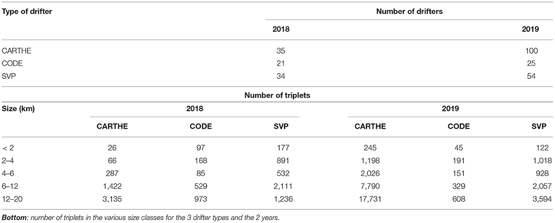
Table 1. Top: number of drifters during the two CALYPSO experiments in May 28 - June 29, 2018 and March 28 - April 29, 2019.

All drifters transmitted their GPS data (and other ancillary data) via either Iridium (SVP) or GlobalStar (CARTHE and CODE) satellites, every 5 or 10 min. Only the drifter GPS position data were considered for this work. The positions were edited for outliers (manually and using automatic procedures based on speed and acceleration criteria) and were linearly interpolated at 5 min intervals. Velocities were estimated by finite differencing the successive positions (central difference over 10 min). The positions and velocities were also low-pass filtered with a Hamming filter, producing two filtered data sets with cut-off at 30 min and 1 h, respectively. In the following analysis the quality-checked unfiltered data set is primarily used, while the filtered datasets have been considered to test the sensitivity of results to very short-time variability.

2.2. Ancillary Datasets

2.2.1. Underway CTD Data

As part of the CALYPSO field campaigns (Mahadevan et al., 2020b), Underway-CTD (UCTD, Rudnick and Klinke, 2007) probes were used to measure vertical profiles of conductivity, temperature and pressure while achieving closely spaced measurements in the horizontal along the ship's track. Free-falling UCTD downcasts (0–300 m depth) were processed for pressure adjustments, sensor alignment and were binned vertically through spline interpolation at 0.5 m resolution (Dever et al., 2019; Mahadevan et al., 2020a). Derived quantities such as practical salinity, absolute salinity, conservative temperature and in-situ density were computed using the Gibbs-Seawater package (McDougall and Barker, 2011). Among the UCTD transects collection we selected one typical transect for each year (2018 and 2019) to illustrate the stratification conditions during each experiment.

2.2.2. Satellite Altimetry Data

Satellite altimetry observations are retrieved from Copernicus Marine Service-CMEMS ocean product catalogue (http://marine.copernicus.eu). The product used here is the “Mediterranean Sea Gridded L4 Sea Surface Heights and derived variables, reprocessed since 1993” (SEALEVEL_MED_PHY_L4_REP_OBSERVATIONS_008_051). Gridded maps of Absolute Dynamic Topography (ADT) are produced by merging all altimeter missions through optimal interpolation of the along-track data. The geostrophic currents are then derived from ADT via geostrophic balance. The ADT and geostrophic current maps for the Western Mediterranean Sea are used here to assess the large and mesoscale circulation during the CALYPSO experiments in 2018 and 2019.

2.2.3. Wind Data

Wind conditions during the CALYPSO experiments are retrieved from the ERA-5, ECMWF atmospheric reanalysis (https://www.ecmwf.int/). Gridded wind fields at 10 m above sea level have 0.28° spatial resolution and 1 h time resolution. Time series of wind speed and direction during the experiment periods in 2018 and 2019 are calculated through spatial averaging over the area covered by drifters (Figures 1, 2).

FIGURE 1

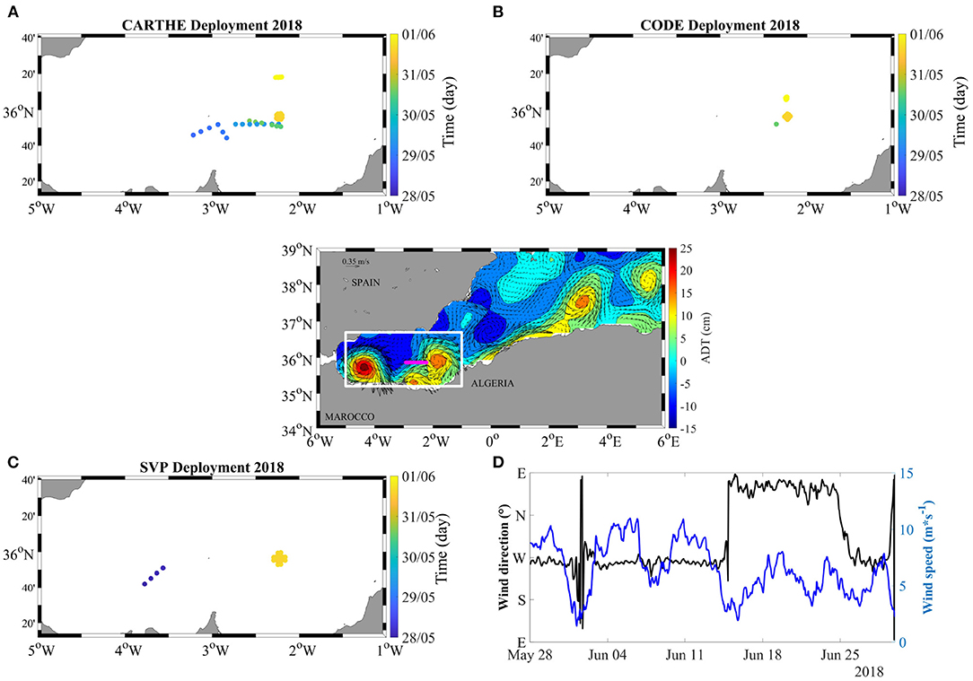
Figure 1. Central panel: mean ADT (units in cm) and surface geostrophic current (black arrows) in the Alboran Sea from May 28 to June 29, 2018. The white box indicates the area of drifter deployments, the magenta line represents the position of the UCTD transect shown in Figure 3. The inserts (A–C) show the color coded deployment sequence of CARTHE, CODE, and SVP. Panel (D) shows the wind speed (blue) and direction (black) time series, averaged over the white box coverage in the central panel.

FIGURE 2

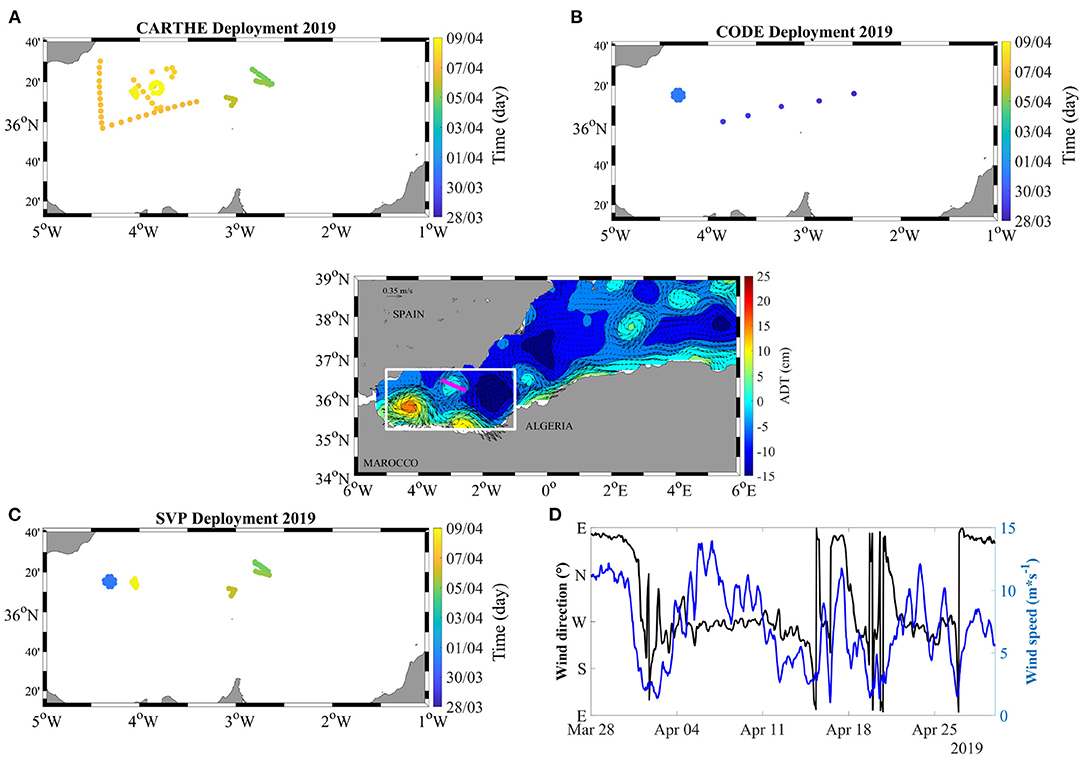
Figure 2. Central panel: mean ADT (units in cm) and surface geostrophic current (black arrows) in the Alboran Sea from March 28 to April 29, 2019. The white box indicates the area of drifter deployments, the magenta line represents the position of the UCTD transect shown in Figure 4. The inserts (A–C) show the color coded deployment sequence of CARTHE, CODE, and SVP. Panel (D) shows the wind speed (blue) and direction (black) time series, averaged over the white box coverage in the central panel.

2.3. Area of Interest and Drifter Deployment

Here, we focus on drifter data taken during the two CALYPSO experiments in the periods May 28–June 29 in 2018 and March 28–April 29 in 2019, respectively. In order to provide a framework for the drifter results, we first characterize the two periods in terms of average ADT, mesoscale dynamics, and associated geostrophic velocity (Figures 1, 2) in the area covered by the drifters. We also show the typical stratification during the two periods (Figures 3, 4) as measured by UCTD sections during the CALYPSO cruises.

FIGURE 3

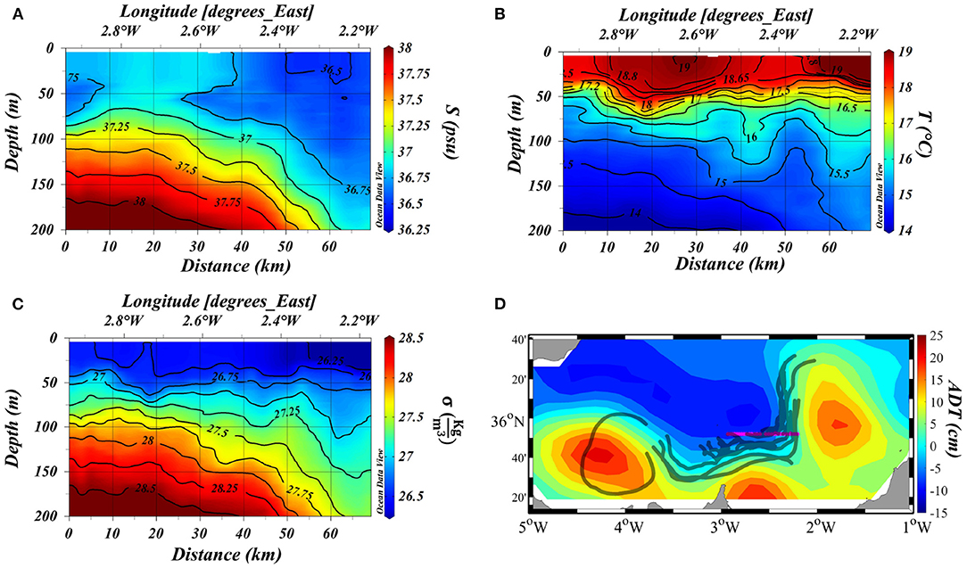
Figure 3. UCTD transect (28–31 May) of salinity (A), temperature (B), and potential density (C) from the CALYPSO experiment 2018. Panel (D) shows the 4-day mean ADT, together with the position of the transect (in magenta, also shown in Figure 1), and drifter trajectories (CODE, CARTHE, and SVP) during the transect time window.

FIGURE 4

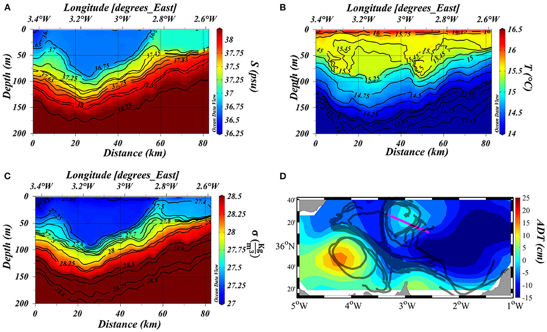
Figure 4. UCTD transect (2–5 April) of salinity (A), temperature (B), and potential density (C) from the CALYPSO experiment 2019. Panel (D) shows the 4-day mean ADT, together with the position of the transect (in magenta, also shown in Figure 2), and drifter trajectories (CODE, CARTHE, and SVP) during the transect time window.

The Alboran Sea is known to be characterized by vigorous and semi-permanent mesoscale dynamics with anticyclonic eddies and associated strong density fronts (Gascard and Richez, 1985; Tintore et al., 1988; Benzohra and Millot, 1995). In particular, the Western Alboran Gyre (WAG) is typically present in the most western side of the basin, while the more variable Eastern Alboran Gyre (EAG) is located more to the East at the boundary with the Algerian basin.

During the 2018 experiment, centered on the month of June, the average mesoscale field shows a well-defined WAG and EAG (Figure 1), with a connecting boundary current and a smaller anticyclone between them along the African coast at approximately 2°-3°W. Another anticyclone is present further East, along the Algerian current around 3°-4°E. The meteorological conditions during the period of interest are characterized by mostly moderate winds (Figure 1), with average speed ≈ 6.5 m/s over the area of interest, reaching ≈ 10 m/s during three meteorological events. The wind direction is mostly zonal (Macias et al., 2016; Oguz et al., 2017). An example of the stratification during the experiment is shown along a section perpendicular to the western side of the EAG, in terms of Temperature (T), Salinity (S), and potential density (Figure 3). The results are typical also of the other sampled sections during the experiment (not shown). A surface mixed layer can be seen in the first ≈ 50 m, mostly driven by temperature that reaches ≈ 19°C at the surface. There are indications of shallower (around 20–25 m) frontal structures in the density within the mixed layer, that reflect horizontal gradients in both T and S, likely due to filaments of Atlantic and Mediterranean waters (see for example ≈ km 18 and 55 in the transect in Figure 3). We also notice the sharp pycnocline sloping between 100 and 200 m, that is associated to the anticyclonic mesoscale eddy.

During the 2019 experiment, centered on the month of April, the ADT average field (Figure 2), shows a well-defined WAG while the EAG is not developed. Several smaller anticyclones can be seen, one along the African coast around 3° W (as in the 2018 experiment), a weaker one more to the East off the African coast around 1° W, and one in the open sea around 3°W, 36° 30′ N. The wind during the 2019 experiment has ≈ 7 m/s mean speed, similar to the 2018 experiment, but is characterized by higher variability in direction and amplitude, with maximum values of almost 15 m/s. The stratification sampled during the 2019 experiment is different from the 2018 experiment, possibly because of interannual seasonal processes or because of local variability. A typical section across the open sea anticyclone is shown in (Figure 4). Compared to the 2018 section (Figure 3), there is no well-defined surface mixed layer in the upper 50 m, (even though the surface is starting to warm up reaching ≈ 16.5°C), and the main pycnocline tends to outcrop to the surface at the edge of the gyre. On the other hand, there are also some similarity with the 2018 surface stratification, in that density gradients are also present in the upper ocean (≈ 20–30 m) away from the outcrop region (see for instance around km 8 in Figure 4). As for June 2018, these surface fronts are likely to be associated to the presence of filaments of water of different Atlantic and Mediterranean origin (Lodise et al., 2020; Tarry et al., 2021). A similar picture, characterized by surface outcropping of the isopycnals around the edge of the mesoscale gyres and smaller surface density gradients occurring away from the outcrop, is commonly observed also in the other 2019 sections (not shown).

The deployment sites for the three types of drifters are shown separately in the panels of Figures 1, 2, color coded with time. The launching strategy involves both extended transects along targeted features, and cluster releases at different depths.

2.4. General Methodology for Computing KPs From Drifters

In this study we focus on the estimate of divergence and vorticity (KPs) as statistical trademark of submesoscale activity in the area of interest, since submesoscale processes are typically characterized by positive vorticity and convergence. A number of methods have been proposed in the literature to estimate KPs from drifter clusters. Most of them are based either on Least Square velocity estimation or on area rate of change estimates (Molinari and Kirwan, 1975; Okubo et al., 1976; Kawai, 1985), using clusters with a minimum configuration of three drifters.

Here we use the area rate of change method (Saucier, 1953; Molinari and Kirwan, 1975; Berta et al., 2016) and the smallest configuration, provided by drifter triplets, chosen because it is more flexible to resolve small scales. The computation is based on the fact that divergence can be expressed as the rate of change of the area of a water parcel, in our case represented by the triangular area delimited by the drifter triplet. The formulation for vorticity can be written in an analogous form, under appropriate rotations of the velocity vectors associated to the vertices of the triangle. Even though estimate precision increases with increasing number of drifters (Essink, 2019), the recent work by Berta et al. (2020b) has shown that statistical estimates from triplets are robust, based on the comparison with estimates from larger drifter clusters and from concurrent independent observations based on Eulerian X-band radar. These findings are also confirmed by modeling results by Sun et al. (2020).

In the following, we show results from estimates of horizontal divergence

$\begin{array}{ll}\delta =\frac{\partial u}{\partial x}+\frac{\partial v}{\partial y};\text{ estimated as }\delta =\frac{1}{A}\frac{DA}{Dt};& (1)\end{array}$

and vertical vorticity component

$\begin{array}{ll}\zeta =\frac{\partial v}{\partial x}-\frac{\partial u}{\partial y};\text{ estimated as }\frac{1}{A^{\prime }}\frac{D{A}^{\prime }}{Dt},\text{ with }u\to -v^{\prime }\text{ and }v\to u^{\prime }& (2)\end{array}$

where u, v are the x, y components of drifters' velocity, computed from triplets evolution during a time step Dt. Drifter triplets are re-sampled every 15 min (only triplets sharing at most one drifter are considered) and followed for the time interval Dt over which the KPs are estimated. Using independent chance triplets for a short time window, instead of following original triplets for longer time, allows to maximize the statistics and to minimize the effect of inhomogeneous sampling driven by convergent regions (Pearson et al., 2020; Sun et al., 2020). The KPs results presented in the following are expressed in terms of the local Coriolis parameter, f (8.572 × 10⁻⁵s⁻¹ at the reference latitude 36° N). KPs triplet-based estimates are valid as long as triplets maintain non-collinear configuration, while they deteriorate as triangles elongate. The aspect ratio of the triangles is evaluated at each time step using the deformation metric λ (Berta et al., 2016, 2020b)

$\begin{array}{ll}\lambda =12\sqrt{3}A/P^2,& (3)\end{array}$

where A and P are the area and perimeter of the triangle, respectively. The λ normalization ensures that λ=0 for collinear triangles and λ=1 for equilateral triangles.

For the purpose of investigating scale dependency of KPs, we separate triplets in selected classes of scales, depending on their size—i.e., the average side length (Berta et al., 2020b). The processes of class selection and KP estimation is performed in such a way to minimize possible error sources, as discussed in the following.

A main error source is the tendency toward deformation and alignment of the triplets since KPs estimation becomes unreliable when clusters tend toward collinearity (Berta et al., 2016; Ohlmann et al., 2017). In order to minimize this error, we perform a targeted triplet selection similarly to what was done in Berta et al. (2020b). At each time interval (15 min), we resample the data set choosing chance triplets of various class sizes that are quasi-equilateral, i.e., with values of λ greater than the cutoff value λ=0.7.

The other main potential error source is due to the GPS error on drifters' position, that is of the order of ≈ 10 m. In order to avoid error propagation from this source, we choose a time step Dt for the estimation of δ and ζ such that the increment in triplet size Dr during Dt is much larger than 10 m. Details on uncertainty estimation from GPS error are provided in the Supplementary Material, while the implementation of the procedures are provided in the next subsection.

2.5. Implementation and Sensitivity Tests

As mentioned in section 2.1 the drifter data sets are available in three different formats depending on data treatment and filtering. The sensitivity of the KPs estimates to these formats and to the choice of Dt has been tested. As a first step, we have chosen a “benchmark configuration” that consists of the quality-checked unfiltered data set, from which KPs are computed using Dt = 30 min.

Triplets at different scales are selected from the data set as mentioned in section 2.4. The various classes of scales are chosen to maximize spatial resolution still retaining a statistically significant number of triplets, leading to a set of classes centered around values of 1, 3, 5, 9, and 16 km. Higher resolution classes, centered at less than 1 km, cannot be achieved because of the restricted number of triplets. The number of triplets in each class for each drifter type is shown in Table 1, bottom panel. KPs for each type of drifter (CARTHE, CODE, and SVP) are then computed for each size class and statistics are evaluated when the number of triplets is larger than a cutoff value of 85.

A few outliers have been removed (approximately 10 points for each type of drifter over thousands of samples), corresponding to isolated points outside the KP distributions. Typical values of Dr corresponding to Dt=30 min are evaluated as averages for each class, and in all cases they are found to be greater than 100 m, which is significantly bigger than the GPS error of 10 m (see also the Supplementary Material).

The robustness of the benchmark configuration is then tested using as metric the root mean square (rms) of the divergence δ (that is one of the main statistics considered in this study), and considering the sensitivity to the formats of the data sets and to different values of the time step Dt. The following tests have been considered:

• The benchmark results obtained using the unfiltered data set have been compared with results obtained using the data set filtered at 30 min. The difference is on average less than 5% in all cases.

• The benchmark results obtained using Dt = 30 min have been compared with results using Dt = 1 h. The difference is less than approximately 10% in all cases. For Dt = 2 h the differences are more significant, as it can be expected given that the time scale of divergence fluctuations is of the order of a few hours.

Overall, the results show that the benchmark configuration is robust, and that minimizes the impact of errors on the estimates. We therefore confirm the use of the benchmark configuration, i.e, the unfiltered dataset and the time step Dt=30 min to compute KPs, and from now on we refer to these results only.

3. Results

3.1. Geographic Distribution of Trajectories and Energetics

We start by providing a general description of the distribution of the trajectories, that are shown in Figure 5 color coded according to drifters' speed (the superimposed black dots indicate triplet distribution, that will be discussed in the next sections).

FIGURE 5

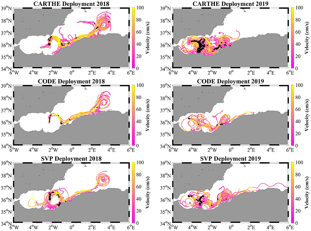
Figure 5. Trajectories of drifters CARTHE (top), CODE (middle), and SVP (bottom) during the experiments 2018 (left) and 2019 (right), color coded with drifters' speed. Black dots represent the spatial distribution of triplets in the range (4–6) km for each type of drifter in each year.

For both experiments, drifter trajectories show a good qualitative agreement with the main features of ADT in Figures 1, 2. During June 2018, the trajectories from the three drifter types sample the EAG and the eastern anticyclone in the Algerian current, while SVPs also partially sample the WAG. During April 2019, all drifter types sample the WAG and the African boundary current with the two smaller eastern anticyclones close to the coast. They also sample the small open ocean anticyclone at around 3°W, 36° 30' N, especially for the CARTHE drifters.

The energetics of the two experiments are similar, but stronger for 2018 probably because of the prevalence of the strong WAG and EAG gyres as shown also in the altimeter maps. Mean speeds are similar for the three types of drifters (CARTHE, CODE, and SVP) and have average values of ≈ 45 cm/s in 2018 and ≈ 40 cm/s in 2019.

3.2. Estimates of Divergence and Vorticity at Different Scales and Depths

In this section, we use the methodology described in section 2.4 and 2.5 to compute divergence and vorticity using triplets in the various classes of scales shown in Table 1, bottom panel. We notice that the number of triplets, especially for small scales, depends not only on the number of drifters (Table 1, top panel), but also on the details of the deployment (see Figures 1, 2). A typical spatial distribution of triplets is shown in Figure 5, considering as an example the positions (black dots) of triplets in the 5 km class characterized by higher divergence values, exceeding 0.5f. The 5 km class, corresponding to the range (4–6) km, has been chosen because is the smallest range with enough data to provide significant statistics for the three drifter types in both years. In the 2018 experiment, the triplets are mostly found along the front of the EAG (left panels) especially for SVPs. CARTHE and CODE triplets are also seen along the African boundary current reaching the eastern anticyclone in the Algerian Current. In the 2019 experiment (right panels) triplets are found in the WAG, in the African boundary current and in part of the open ocean smaller anticyclone around 3° W,36° 30' N.

As a first step in the analysis, we investigate the possibility of computing the statistics separately for the three drifter data sets. Specifically, the question that we address is whether or not there are enough data to significantly differentiate between the very surface drifters, i.e., CARTHE at 60 cm and CODE at 1 m. Previous works have shown the presence of significant shears in the first meter of water (Laxague et al., 2018; Lodise et al., 2019), suggesting that it would be interesting to keep them separate, but the number of data is limited, so that a preliminary investigation is needed.

We consider two classes of triplets as examples, one at the smallest resolved scale of 1 km (range <2 km), and the other at the larger 9 km scale (range 6–12 km), and we investigate the KP statistics, comparing the two surface drifters and the 15 m SVPs. Probability density functions (Pdfs) of divergence and vorticity are shown in Figures 6, 7, respectively, for the two classes and the 2 years. The corresponding statistics are shown in Table 2. As shown in Table 1, bottom panel, in both years for the smallest class (<2 km) only one type of surface drifters has sufficient data for analysis (i.e., more than 85 values) : CODE for 2018 and CARTHE for 2019.

FIGURE 6

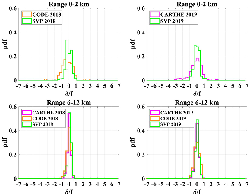
Figure 6. Distribution of normalized divergence estimates for the 3 types of drifter (magenta for CARTHE, orange for CODE, and green for SVP) during the experiments 2018 (left) and 2019 (right) calculated from drifter triplets in the ranges: <2 km (upper) and (6–12) km (lower).

FIGURE 7

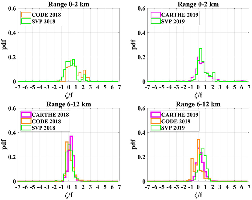
Figure 7. Distribution of normalized vorticity estimates for the 3 types of drifter (magenta for CARTHE, orange for CODE, and green for SVP) during the experiments 2018 (left) and 2019 (right) calculated from drifter triplets in the ranges: <2 km (upper) and (6–12) km (lower).

TABLE 2

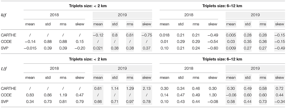
Table 2. Statistical results for the normalized divergence (δ/f) and vorticity (ζ/f) distribution (top and bottom panel, respectively) for the 3 types of drifters in the ranges <2 and 6–12 km for years 2018 and 2019.

For the smallest class (<2 km) the pdfs of divergence (Figure 6 upper panels) show a clear difference between the SVP and the surface drifters considered for each experiment. The SVP distribution is more peaked, while the surface drifters are more spread-out and characterized by higher standard deviation (std) and root mean square (rms) (Table 2, top panel), with individual values reaching 3f. For the vorticity (Figure 7 upper panels), the surface pdfs show prevalent positive values, with significant means (up to 0.8f for CODE 2018), and heavy positive tails especially for CARTHE 2019, with individual values exceeding 6f. The SVP pdfs have qualitatively similar properties but reduced values of std and rms (Table 2, bottom panel). For the larger class (6–12 km) the situation is different (Figures 6, 7 lower panels). For all drifter types and for both KPs, the pdfs are more peaked than for the smaller class. The std and rms values are smaller (Table 2), and there is no clear difference between the distribution of SVPs and the more surface drifters. The vorticity distribution is positively skewed for both classes and for both surface drifters, as it can be expected in presence of submesoscale processes in an area with strong lateral gradients and frontogenesis. For SVPs the skewness is positive for the smaller class, and slightly negative at the bigger scales. The divergence skewness is smaller than for vorticity and less well-defined, even though mostly negative.

Overall, the results indicate that the there is no detectable systematic difference between the statistics of the two surface drifter sets at the larger scales of 9 km, while at the smaller scales of 1 km the coverage is insufficient to differentiate among them. Differences with SVPs are comparable for the two surface sets. As a consequence in the following we analyze the two surface drifter data sets together. This allows increasing the number of triplets in each class (Table 1, bottom panel), giving a minimum of 123 surface triplets for the smallest class (<2 km) in 2018 and 290 in 2019.

3.2.1. Results for Surface and 15 m Drifters

In the following we present the results obtained grouping the surface drifters CARTHE and CODE, comparing them with the 15 m results from SVPs, and focusing on KPs main statistics vs. space scale.

We start by analyzing the behavior of the rms values, that are especially interesting since they provide an indication of the typical magnitude of the variables. Figure 8 summarizes the results for both KPs and experiments. Before going into the details of the results, we notice that the different types of drifter triplets sample similar but not exactly coincident features (see example in Figure 5), with the surface drifters extending more toward the Algerian boundary current in both experiments. This implies a potential bias in the comparison between surface and 15 m, due to the differences in sampled regions. In order to gain some insight on this aspect, we performed a preliminary test for the 2018 experiment, considering only data in the EAG anticyclone that is covered by all three types of drifters (Supplementary Figure 1). No significant differences are found, reinforcing the main conclusions discussed below.

FIGURE 8

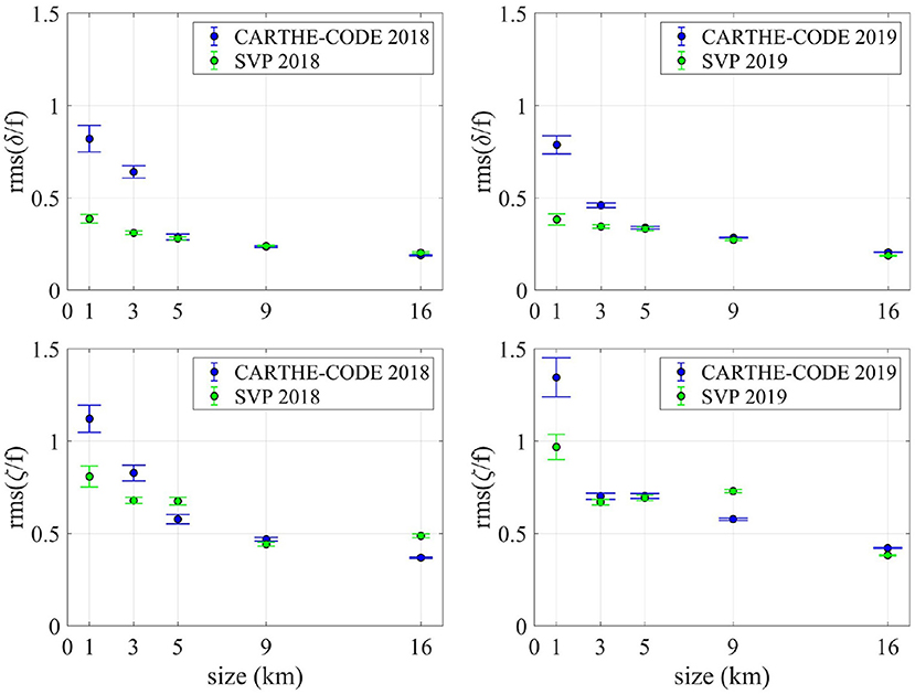
Figure 8. Scale dependence of rms values of normalized divergence (upper) and vorticity (lower) for the experiments 2018 (left) and 2019 (right) for the surface drifters (CARTHE and CODE) in blue and 15 m drifters (SVP) in green. Error bars indicate 95% CI.

For divergence (Figure 8, upper panels), the rms values for surface drifters in both experiments are slightly less than 1f at 1 km, and decrease to approx 0.25f at approximately 10 km. Also, for both experiments, the SVP values are significantly smaller than the surface drifters for scales of 1 km (less than 0.5f), while they are of the same order at bigger scales (>5 km), resulting in a slower decay with increasing scales.

The vorticity scale dependence (Figure 8 lower panels) shows surface values greater than 1f at the smallest scales of 1 km, decreasing to approximately 0.5f at scales of the order of 10 km. Also in this case, SVP values are smaller than surface values at the smallest scales, even though the attenuation is less severe than for divergence. For scales of 5 km or more, the SVP values are the same or greater than the surface ones. The rms trend with scales is influenced by the trend of the mean vorticity values, that are typically positive for surface drifters and SVPs, and reach values of 0.8f at small scales as shown in Supplementary Figure 2, especially for 2019. We note that this is not the case for divergence (Supplementary Figure 3), where mean values are small (not exceeding 0.15f for all scales) and oscillate around 0. The vorticity skewness (Figure 9) shows consistently positive values for surface drifters, exceeding 1 for the 2019 experiment at 1 km. For SVPs, the skewness is still typically positive at small scales, reaching high values close to 1 for the 2018 experiment at 1 km, but there is more variability in the scale results, with some significant negative values (−0.5). On the other hand, for divergence skewness (Supplementary Figure 4) negative values (around −0.5) prevail across the different scales, with a peak for surface drifters at 1 km in 2019 (≈-0.8).

FIGURE 9

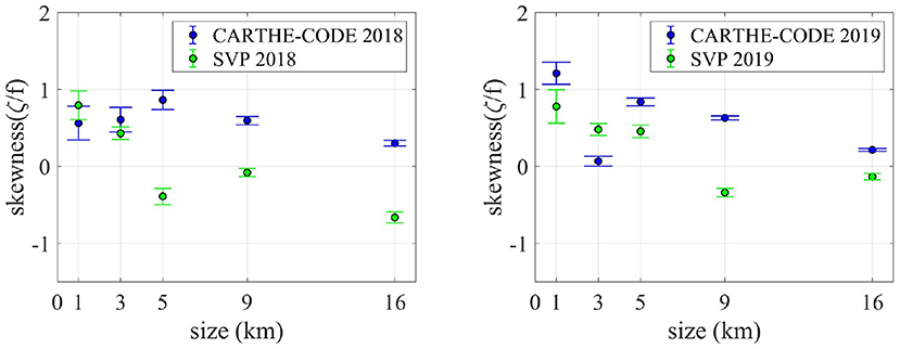
Figure 9. Scale dependence of vorticity skewness for experiments 2018 (left) and 2019 (right) for the surface drifters (CARTHE and CODE) in blue and 15 m drifters (SVP) in green.

The variance vs. scales of the two KPs are shown in a log-log plot (Figure 10) for both experiments together, to facilitate comparison. We also show two slopes for reference: the −4/3 slope, compatible with a second order structure function decaying with scale as r^2/3 (Berta et al., 2020b), typical of a broad band spectrum as in 3d turbulence; and a slower decaying −4/5 slope, also considered in Berta et al. (2020b) for comparison. For divergence, the surface drifters for both experiments show a quick decay, compatible with the −4/3 slope up to approximately 5–9 km. The SVP decay, on the other hand is slower and characterized by a slope closer to −4/5. For vorticity, all the data sets decay more slowly, with a slope close or even less than −4/5, especially for scales greater than 5 km.

FIGURE 10

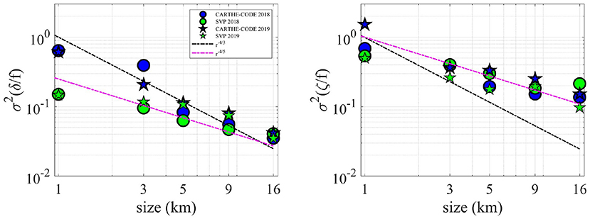
Figure 10. Scale dependence of the variance of divergence (left) and vorticity (right) for both experiments (2018 circles, 2019 stars), and for the surface drifters (CARTHE and CODE) in blue and 15 m drifters (SVP) in green. For comparison, the scaling laws for velocity derivatives are also shown: black line for −4/3 slope and magenta line for −4/5 slope.

The comparison between the results in the two experiments is further investigated computing the joint probability distribution of vorticity and divergence. An example for the range <6 km at the surface is shown in Figure 11. The 2018 results (left panel) show prevalent negative values of divergence at high positive vorticity, which is the expected trademark of submesoscales. The values though are relatively contained and no negative vorticity values exceeding −1f are present. The 2019 results (right panel) are significantly more noisy, with a more extended distribution and heavier tails (compatible also with the results in Figures 6, 7). This suggests the presence of several incidents of more vigorous submesoscale processes with respect to the 2018 experiment. The results at 15 m, on the other hand, do not show significant differences, and are similar for the two experiments (not shown).

FIGURE 11

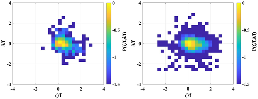
Figure 11. Normalized joint probability distribution of divergence and vorticity (logarithmic scale) for surface drifters (CODE and CARTHE) in the range below 6 km for experiments 2018 (left), and 2019 (right).

3.3. Summary of Results

The results presented above provide an interesting and articulated picture of the upper ocean between the surface and 15 m at horizontal scales of 1–16 km, bridging the meso and submesoscale range. Here we summarize the main findings and point out some interesting open issues.

At the surface, CARTHE and CODE drifters sampling the first meter of water indicate that the flow is highly ageostrophic at scales of 1 km, with typical rms values of order f for both KPs (higher than 1f for ζ and slightly less than 1f for δ) and individual values exceeding 3-6f. Positive vorticity skewness indicates the presence of submesoscale dynamics, in agreement with previous results (Shcherbina et al., 2013). Both surface KP values decrease with increasing horizontal scales, as expected, but there is a significant difference between divergence, that decreases faster with variance slope ≈ −4/3 at least up to scales 5–9 km, and vorticity variance that decreases more slowly, with a slope ≈ −4/5 or smaller, and tends to flatten for scales larger than 5 km, suggesting an interaction with mesoscales. The dynamical reasons behind these different decays will be further discussed in section 4, comparing our results with other literature results.

At 15 m, results from SVP drifters show that the flow has similar but attenuated characteristics with respect to the surface. The attenuation is especially evident for divergence, that has rms values less than 0.5f at 1 km and significantly slower decay with scales with respect to the surface, suggesting that the flow is less dominated by small scales. The vorticity shows similar but less marked results, with rms below 1f at 1 km and reduced scale dependence. The skewness values are positive at the smallest scales, but there is more variability with scales, with the occurrence of some negative values. This indicates that the flow is still ageostrophic but the influence of submesoscale processes is attenuated with respect to the surface.

From the dynamical point of view, the attenuation with depth points to the relevance of boundary layer processes (D'Asaro, 2014) that are expected to energize surface dynamics, increasing divergence and vorticity and influencing the smaller scales. This is indeed in agreement with TTW and TTTW results, that indicate that ageostrophic overturning is intensified in presence of strong vertical turbulence and lateral buoyancy gradients (Dauhajre et al., 2017). Also the presence of Langmuir cells, that can reach scales of 1 km (Malarkey and Thorpe, 2016; Suzuki et al., 2016) is expected to increase surface kinematic properties, as well the interaction between fronts and waves (McWilliams and Fox-Kemper, 2013; Suzuki et al., 2016). The wave interaction occurring through Stokes shear forces, can inject energy and momentum at the scales of the front, i.e., well beyond the actual scales of Stokes drift. Finally, ageostrophic overturning in shallow mixed layer fronts have also been shown to evolve in surface gravity currents (Pham and Sarkar, 2018), with strong across front velocities. All these results provide a useful general framework that goes in the direction of explaining the present results. There are some specific questions, though, that are still not resolved at least at the authors knowledge, and need further investigation. For instance it is not clear whether high wind stress directly correlates with enhanced surface values of KPs and with depth attenuation in the upper 15 m. Some mechanisms, such as the dependence of the overturning circulation on vertical mixing suggests that high wind stress induces higher surface KPs, but other mechanisms such as Ekman pumping (Thomas et al., 2013) and wave interactions (Suzuki et al., 2016) can act both ways, since they depend on the specific wind direction with respect to the front. Also other mechanisms related to atmosphere feedback to submesoscale fronts can act both ways (Renault et al., 2018). A statistical answer based on the present data set is not feasible, because there are not enough information on triplet sampling with respect to frontal structures nor enough co-located triplets. Further studies would be necessary to address these questions either considering specific events (Johnson et al., 2020a,b), or using model results (Oguz et al., 2017). Another interesting question arises from the difference in the attenuation of ζ and δ. A possible hypothesis is that higher values of ζ at larger scales and at depth are sustained by mesosocale interactions. Again, further studies are necessary to quantitatively address these points.

The results on scale and depth dependence are generally valid for both experiments, but it is interesting to verify whether there are some quantitative differences between them related to the different environmental characteristics, especially in terms of stratification.

Comparing the 2018 and 2019 results, differences can indeed be seen in the surface δ and ζ joint probability density (Figure 11). The flow in the 2019 experiment presents more extreme values of vorticity and divergence, suggestive of the occurrence of stronger submesoscale events, in agreement with the different stratification characteristics and possibly also with the higher wind effects. The bulk statistics, though, are similar for both experiments, and the 15 m attenuation of submesoscale signatures is seen in both cases, even though is slightly more evident in the 2018 experiment, as indicated by the more variable skewness.

A possible hypothesis to explain the limited statistical differences, despite the stratification differences shown in Figures 3, 4. is that submesoscale instabilities might occur mostly within the shallower filamentations with depth of ≈ 25–30 m, that are indicative of different water masses and that are present during both experiments (Lodise et al., 2020; Tarry et al., 2021). Even though an in depth investigation of the effects of stratification is out of the scope of this paper, we have quantitatively tested this hypothesis characterizing the stability properties (Thomas, 2008) of the two sections in Figures 3, 4 in the upper 50 m, computing the vertical and lateral buoyancy gradients, N² and M², and the balanced Richardson number $R{i}_B=f^2{N}^2/M^4$ (see Supplementary Figures 5, 6). Values of Ri_B smaller or close to 1 are typical of submesoscale regimes, and indicate regions prone to frontal instabilities such as symmetric instabilities (SI) (Taylor and Ferrari, 2010), forced symmetric instabilities (FSI) (Thomas et al., 2013), and ageostrophic baroclinic instabilities (ABI) (Boccaletti et al., 2007). The results in Supplementary Figures 5, 6 show values of N² and M² reaching 10⁻⁴ and 10⁻⁶ s⁻², respectively, for both experiments, in the range of previously observed values in submesoscale regimes (Thompson et al., 2016; Ramachandran et al., 2018; Johnson et al., 2020a,b). Also, while regions with Ri_B < 1 are restricted especially for the 2019 section, values close to 1 can be seen in both years. Actually, even though M² reaches the highest values in the outcrop region in 2019, values of Ri_B close to 1 are indeed more prominent in 2018, close to the surface filaments shown in Figure 3. These results therefore reinforce the fact that water masses gradients support submesoscale processes in both experiments.

Also, another factor to be considered is that the statistical description at scales of order of 1 km, as considered here, might not be sufficient to effectively diagnose the complete development of submesoscale frontal phenomena. Recent studies have shown that frontal structures are characterized by scales of the order of hundred to tens of meters and values of KPs of the order of tens of f (Gonçalves et al., 2019; Lodise et al., 2020). We will come back on this point in section 4 in the framework of literature comparison.

4. Discussion

In this section, we compare our main findings on KP dependence on depth and horizontal scales with previous results reported in the literature, with the goal of contributing toward a synthesis of experimental results and identification of open questions.

4.1. Comparison With Previous Results on Depth Dependence

We start by comparing our statistical results on depth dependence over the first 15 m with results obtained by Tarry et al. (2021) using the same CALYPSO data set, but focusing on a specific event in June 2018, sampled also by a neutrally buoyant Lagrangian float (D'Asaro, 2003). Tarry et al. (2021) analyze a submesoscale instability at a surface front, where the mixed layer was about 15 m deep in the dense part, shallowing to less than 6 m at the front and then reaching 20 m in the lighter part. KPs estimates during the event show vorticity values reaching approximately 2f at the surface and barely 1f at 15 m. A strong convergence signal of approximately 2f is observed at the surface, while at 15 m divergence reaches 0.5f and does not show any obvious correlation with the surface. Indeed, measurements of vertical velocity from the float indicate that the divergence is not a linear function of depth between the surface and 15 m. A very high spatial variability in KP values is found at the surface, while at 15 m the values are smoother. Overall, the description of this specific event is in good agreement with our statistical findings, that indicate a decrease of small scale KP values at 15 m, especially evident for divergence, and increased variance at scales of the order of 10 km, indicating smoother divergent patterns.

Surface intensification of submesoscale KPs in the upper ocean has also been observed during a 1-day survey with a ship-towed Triaxus profiler in the California current (Johnson et al., 2020a). Vorticity and divergence were inferred at several depths in the first 20 m and in the layer 100–140 m, showing strong fluctuations in time and approaching values of order f near the surface.

Other experimental results in the literature regarding KPs variability do not resolve the upper ocean in the first 15 m. Statistical submesoscale depth dependence has been studied by Shcherbina et al. (2013), Buckingham et al. (2016) in the North Atlantic comparing currentmeter observations in the range of 50 m with deeper results at 350–500 m depth. In winter, when the mixed layer depth is deeper than 50 m, they report attenuation of KPs std of approximately a factor two and a marked difference in the shape of vorticity pdfs, with skewness values exceeding 1 at 50 m and decreasing to values close to zero at depth.

4.2. Comparison With Previous Results on Horizontal Scale Dependence

Our statistical results on the KPs dependence on horizontal scales are first compared with previous results by Berta et al. (2020b), obtained in a different part of the world ocean, i.e., in the surface Northern Gulf of Mexico (GoM), using a similar drifter analysis and covering a (partially) compatible range of scale. We notice, though, that the drifter sampling strategy in Berta et al. (2020b) is different from the one used here. While in the present analysis chance triplets over an extended geographical region and during 1 month period are used, providing an “average” picture of the dynamics in the Alboran Sea region, Berta et al. (2020b) consider short analysis periods of 1–3 days, providing a more synoptic description of specific environmental situations. The analysis is based on massive cluster deployments (order of 100–300 drifters) synoptically launched during the CARTHE experiments in 2012 and 2016 (D'Asaro et al., 2020), that specifically targeted submesoscale dynamics in a GoM area influenced by the Mississippi outflow. Four main releases are analyzed in Berta et al. (2020b), two during summer (S1, S2) and two during winter (W1, W2), characterized by different conditions. In particular, the winter W1 deployment targeted an energetic cyclonic eddy of approximately 20 km in diameter, characterized by strong surface density gradients associated with filaments of fresh Mississippi River water, while the W2 deployment occurred in an area with nearly homogeneous horizontal density during the onset of a storm with high winds.

In Figure 12, the scale dependence of the variance of δ and ζ are shown in a range between 0.2 and 16 km, covering both the Berta et al. (2020b) and our results. The scale dependence of divergence variance (Figure 12 upper panel) is quite consistent in all cases with an approximately −4/3 slope up to 5–9 km scales. The GoM summer values are the lowest, as it can be expected given the very shallow mixed layer in this area (5–10 m), while the two GoM winter cases are in the same range as the two Alboran Sea cases considered here. Overall, the consistency of results despite the differences in geographical and dynamical regions is noteworthy. In particular, the consistency with the W2 case, obtained in environmental conditions indicating weak submesoscale instabilities and strong wind effects (Berta et al., 2020b), suggests the importance of boundary layer dynamics in shaping divergence scale dependence.

FIGURE 12

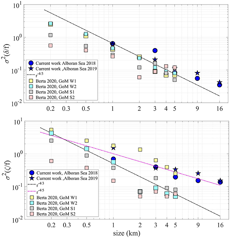
Figure 12. Scale dependence of the variance of divergence (upper) and vorticity (lower) for surface values from Berta et al. (2020b) in the Gulf of Mexico (GoM) and from present results. For comparison, the scaling laws for velocity derivatives are also shown: black line for −4/3 slope and magenta line for −4/5 slope.

The vorticity variance (Figure 12 lower panel) shows a more complex situation. Summer GoM and the winter W2 cases have lower vorticity variance and show a quick decay with scales, compatible with the same −4/3 slope as divergence. The GoM W1 and the two Alboran Sea cases, on the other hand, are characterized by higher variance values and slower decay (−4/5). This suggests an interaction with larger scale vorticity, and possible mesoscale transfer fueling vorticity values at intermediate scales (Lodise et al., 2020).

Scale dependence of KPs have also been considered by Ohlmann et al. (2017) using surface drifters in the coastal California currents, based on repeated small cluster deployments targeting coastal eddies and frontal features. Ohlmann et al. (2017) consider the scale dependency of mean square (ms), rather than variance, in a range covering approximately 400 m–3.5 km (their Figure 5). The comparison between our ms results and the Ohlmann et al. (2017) ones is therefore limited to 2 data points, corresponding to approximately 1 and 3 km scales. A qualitative comparison of ms values shows that δ and ζ values are in the same range, but the Ohlmann et al. (2017) values are consistently higher. The values are 1.2f and 2.5f for δ and ζ at 1 km (vs. 0.7f and 1.6f in the Alboran Sea), and 0.3f and 1f at 3 km (vs. 0.25f and 0.5f). The difference is at least partially due to the fact that the California Current deployments were targeted to eddies and fronts, that are characterized by high KP values. The ratio between 1 km and 3 km values are in the range of 2.5–3 in all cases, except for the divergence in Ohlmann et al. (2017), that has a 4 ratio, suggesting a faster decay at those scales. Indeed Figure 5 of Ohlmann et al. (2017) shows a very fast decrease of δ for scales greater than 1 km, while ζ oscillates and decreases slowly. The difference between the δ and ζ decay is consistent with our findings, but even more marked. We also mention that scale dependence has been considered by Johnson et al. (2020a) using Triaxus and SEASOR data at scales of 5 and 12 km during the frontal survey in the California current. Even though the methodology is quite different, they find consistent values (of order 0.7f at 5 km and 0.1f or less at 10 km) with more pronounced scale decay for δ.

4.3. Outlook on Small Scales and Frontal Events

The statistical properties presented here provide a description of KP properties at a given scale between 1 and 16 km. As discussed in section 3.3, though, the characteristics of specific frontal events might need a more detailed description, likely including smaller scales. Lodise (2020) has recently proposed that values of maximum vorticity and divergence could provide useful metrics to characterize frontal events, and has provided a literature overview (his Figures 3.20, 3.21) of such values for scales smaller than 1 km, considering various types of instrumentations and methodologies. Here we report the Lodise (2020) results in our Figure 13, integrated with results from the present study in the Alboran Sea at 1 km and from Berta et al. (2020b) in the GoM at the available scale of 500 m (their Figures 10, 11).

FIGURE 13

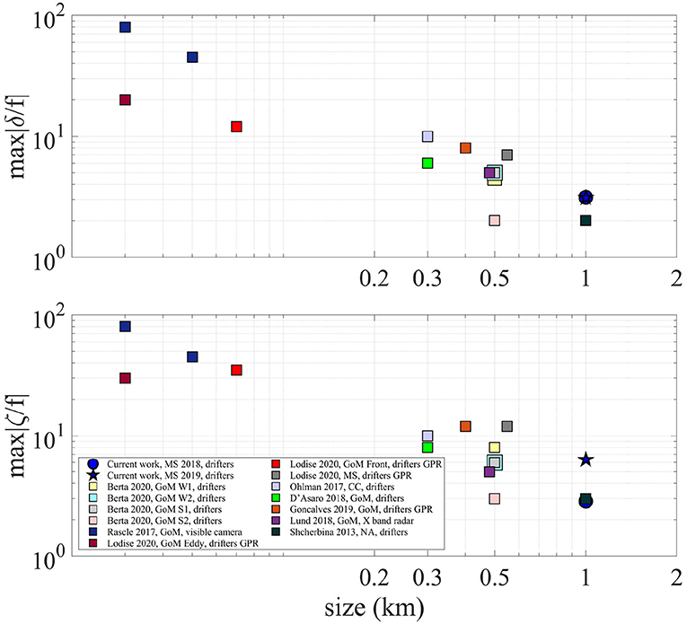
Figure 13. Scale dependence of the maximum divergence (upper) and maximum vorticity (lower) for surface values from the literature and from present results. Adapted from Figures 3.20, 3.21 by Lodise (2020).

The results in Figure 13 have been taken in various world oceans, including the Gulf of Mexico, North Atlantic, California Current, and Mediterranean Sea (see legend). They are mostly obtained from surface drifters, aside from Shcherbina et al. (2013) that are taken from ADCP, Rascle et al. (2017) from visible camera on airborne surveys, and Lund et al. (2018) from shipboard X-band radar (see also Table 5 in Lodise et al., 2020). Also, various methodologies have been used to analyze drifter data, following two main approaches. The first approach, (used in Ohlmann et al., 2017; D'Asaro et al., 2018; Berta et al., 2020b) includes techniques that estimate KPs directly from drifter clusters, provided that the cluster aspect ratio is beyond a certain threshold value. The second approach (used in Gonçalves et al., 2019; Lodise et al., 2020) is based on the reconstruction of the Eulerian velocity field using a Gaussian Process Regression (GPR), from which KPs are then evaluated. While also this technique is limited by drifter availability and cluster deformation, the flow parameter estimation allows a greater flexibility reaching smaller scale estimates.

Figure 13 shows the relationship between maximum δ and ζ values and the horizontal scale of the estimates. For the GPR based studies (Gonçalves et al., 2019; Lodise et al., 2020), the horizontal scale corresponds to the smallest correlation scale evaluated for each analyzed event. The horizontal scales associated with the visible camera measurements made by Rascle et al. (2017) are defined by the two different estimates of the width of front sampled (30 and 50 m). For statistical analyses at relatively coarse resolution (Shcherbina et al., 2013; Ohlmann et al., 2017; Lund et al., 2018; Berta et al., 2020b and the present study), for each class of scale, the maximum values from the distributions of δ and ζ are chosen and plotted against the resolution of the other datasets. Assigning a horizontal scale to the maximum kinematic values found by D'Asaro et al. (2018) is less trivial due to the fact that the ellipses method used becomes less accurate as drifters converge and become less isotropically spaced. Lodise et al. (2020), as well as this study, choose a corresponding length scale of 300 m. Varying this scale between 200 and 500 m still results in good agreement with the trends seen in Figure 13.

Most of the values in Figure 13 are clustered in a range between 300 m and 1 km, where most of the observations are taken. In this range, the maximum divergence values are approximately three times larger than the corresponding variance values in Figure 12 (upper panel), with the summer values in the GoM being distinctively smaller than the others. Despite the fact that the results are obtained from various instruments and in various locations of the world ocean, the divergence trend in this range shows a well-defined quasi-linear decrease at increasing scales, qualitatively consistent also with what shown in the variance plot (Figure 12 upper panel). We notice that the values include also the Alboran Sea estimates by Lodise et al. (2020) with GPR, corresponding to δ approximately 7f at 550 m. A second cluster of values is found for smaller scales in the range 70-30 m, with maximum δ values reaching almost 100f at the smallest scales. The highest values are obtained by Rascle et al. (2017) using visible camera on airborne surveys over the GoM which sampled a very narrow front, 30–50 m in width, followed by GPR estimates at 70 and 30 m also in the GoM. The vorticity plot (Figure 13 lower panel) shows similar general features, even though in the range 300m–1km the values are more scattered, in keeping also with the variance plot (Figure 12 lower panel). The Lodise et al. (2020) estimate for the Alboran Sea reaches 11f at 550 m. The highest values of order 100f are confirmed at 30 m for the camera measurements, while GPR estimates at those scales reach 30f.

Overall the results indicate that there is a good consistency between different types of instruments and methodology at various scales. They also show that frontal features can reach small scales of the order of tens of meters with KPs values of the order of 10–100f, and that targeted techniques are necessary to reach such resolution.

5. Concluding Remarks

In this paper we analyze drifter data at the surface and 15 m in the Alboran Sea during two experiments, one in June 2018 and the other in April 2019. We use drifter triplets at various scales during 1 month period to investigate the statistics of vorticity and divergence as function of horizontal scales and depth in the upper mixed layer. We span the range between 1 and 16 km, that bridges the submesoscale and mesoscale, in an area characterized by strong mesoscale variability. Results are compared with other literature results in several regions of the world ocean and obtained with different methodologies, in an effort to provide a synthesis of results and identify open issues and new avenues of investigation.

The surface results (1m depth) show that for both experiments the flow is highly ageostrophic at 1 km scales, in agreement with other results in the world oceans (Shcherbina et al., 2013; Ohlmann et al., 2017; Berta et al., 2020b). The vorticity skewness is positive at all scales, indicating the presence of submesoscale features.

At 15 m, the KPs are qualitatively similar to those at the surface but significantly less ageostrophic (especially for divergence), in agreement also with what was found by Tarry et al. (2021) in the analysis of a specific event during the 2018 experiment.

Both δ and ζ statistics decrease with scales, even though at different rates. The decay is faster for δ at the surface as observed also in other results in the California Current (Ohlmann et al., 2017) and in the GoM (Berta et al., 2020b). In particular, the δ variance decay is consistent with a −4/3 slope, characteristic of a broadband energy spectrum as in 3d turbulence. At 15 m, on the other hand, the decay is slower with a reduced slope smaller than 1. The ζ variance decay both at the surface and at 15 m also shows a slope smaller than 1, similar to previous literature findings in presence of large scale vorticity structures (Ohlmann et al., 2017; Berta et al., 2020b).

Overall, the vorticity scale dependence suggests the interaction of submesoscale processes, that are dominating at the surface and less pronounced at 15 m, with mesoscale processes that sustain vorticity variance at intermediate scales. The faster decay of surface divergence, on the other hand, indicates the strong influence of surface boundary layer processes at scales of few kilometers. This is in agreement with what suggested by a number of modeling and theoretical results on the effects of boundary layer turbulence (Dauhajre and McWilliams, 2018), wind (Thomas et al., 2013), Langmuir cells and waves (Suzuki and Fox-Kemper, 2016; Suzuki et al., 2016) on overturning circulation. The present results provide a quantitative statistical assessment of these effects, and can be seen as complementary to other experimental results focused on specific events (Berta et al., 2020b; Johnson et al., 2020a,b). As such the present results can contribute to provide benchmarks for theoretical and modeling results.

An interesting question is whether the present findings on variance decay with space scales r can be related to wavenumber k spectra (Lien and Sanford, 2019). Simple dimensional considerations would suggest that if the variance decays with space scale as r⁻ⁿ, then the corresponding wavenumber k spectral density varies as k^m, where m = n − 1. This would imply a blue spectrum for n > 1 and a red spectrum for n < 1, with m = −1 for n = 0. On these bases, our findings suggest a blue spectrum for surface divergence, that is influenced by 3d boundary layer processes, while at 15 m, away from the effects of surface dynamics, the spectrum tends to become red. For vorticity, the results suggest red spectra both at the surface and 15 m, probably because of the influence of mesoscale. In particular at 15 m the slope tends to flatten almost to a m = −1 slope at scales of 5–9 km, that is consistent with quasi geostrophic dynamics. While these simple considerations are interesting and suggestive of broad dynamical scenarios, they should be taken with caution and only as qualitative indications. The variance computation at each scale, in fact, is actually aliased by the presence of the smaller scales (Lien and Sanford, 2019; Tarry et al., 2021), and effects of area averaging need to be expressed by appropriate transfer functions and taken into account in order to quantitatively express spectrum slopes. Further investigations are needed to address this point.

Another interesting issue is related to the comparison between the 2018 and 2019 experiments that are characterized by different environmental properties especially in stratification. The KPs show some differences, with increased occurrence of high δ and ζ values in 2019, indicating stronger submesoscale events, possibly related to the stratification outcrops and higher wind events. Nevertheless, there are no consistent differences in the bulk statistics of the two experiments at various scales, and the 15m attenuation is observed in both experiments. This is likely due to the fact that submesoscale instabilities occur mostly at surface fronts associated with filaments, that are present in both experiments due to the mixing of Atlantic and Mediterranean waters that is characteristic of the Alboran Sea. This is suggested also by the occurrence of near unit values of the balanced Richardson number in the vicinity of surface filaments in both years.

Further investigations are planned to address some of the open question. In particular, we are planning to isolate and study in details specific events occurring in the area of the gyre outcrops in April 2019, in order to better understand its dynamics and vertical extent. Recent results (Lodise et al., 2020) show that in order to fully describe frontal processes, high resolution estimates at less than hundred meters might be necessary, with KPs reaching very high values in the range 10–100f. Appropriate methodologies and metrics are necessary to address such scales. Maximum KP values might be useful to identify events (Lodise et al., 2020), while dilation type metrics (Huntley et al., 2015) can be used to quantify their persistency and therefore their relevance for vertical transport. Also the interactions with surface dynamics and high wind effects on drifter trajectories will be further investigated.

Data Availability Statement

The raw data supporting the conclusions of this article will be made available by the authors, without undue reservation.

Author Contributions

GE performed the analysis on the Alboran Sea dataset and contributed to the writing. MB provided the methodology and collaborated to the analysis process and contributed to the writing. JL provided input for comparison with literature and contributed to the writing. LC, P-MP, and TÖ provided the drifter datasets and contributed to the analysis interpretation and to the writing. TJ provided the uCTD dataset and revised the manuscript. AG coordinated the work and led the writing. All authors contributed to the article and approved the submitted version.

Funding

The work has been supported and co-financed by the Office of Naval Research under the CALYPSO Departmental Research Initiative (Grant numbers N00014-18-1-2782, N00014-18-1-2418, and N00014-18-1-2416). LC and the SVP drifters were funded by ONR grant numbers N00014-17-1-2517 and N00014-19-1-269. The analysis methodology has been mainly developed within the CARTHE III project (Prime Award n. SA 18-14, subcontract agreement SPC-000649), under the Gulf of Mexico Research Initiative framework. Investigation of (sub)mesoscale dynamics in the Mediterranean Sea is also supported by the JERICO-S3 project under the European Union's Horizon 2020 research and innovation programme with grant number 871153.

Conflict of Interest

The authors declare that the research was conducted in the absence of any commercial or financial relationships that could be construed as a potential conflict of interest.

Acknowledgments

The authors thank the CALYPSO team and the cruise participants in 2018 and 2019 experiments.

Supplementary Material

The Supplementary Material for this article can be found online at: https://www.frontiersin.org/articles/10.3389/fmars.2021.678304/full#supplementary-material

Footnote

1. ^Poulain, P.-M., Centurioni, L., and Ozgokmen, T. (under review). Comparing the currents measured by CARTHE, CODE and SVP drifters as a function of wind and wave conditions in the southwestern Mediterranean Sea. J. Atmos. Ocean. Technol.

References

Barkan, R., Molemaker, M. J., Srinivasan, K., McWilliams, J. C., and D'Asaro, E. A. (2019). The role of horizontal divergence in submesoscale frontogenesis. J. Phys. Oceanogr. 49, 1593–1618. doi: 10.1175/JPO-D-18-0162.1

CrossRef Full Text | Google Scholar

Benzohra, M., and Millot, C. (1995). Hydrodynamics of an open sea Algerian eddy. Deep Sea Res. I Oceanogr. Res. Pap. 42, 1831–1847. doi: 10.1016/0967-0637(95)00046-9

CrossRef Full Text | Google Scholar

Berta, M., Corgnati, L., Magaldi, M. G., Griffa, A., Mantovani, C., Rubio, A., et al. (2020a). Small scale ocean weather during an extreme wind event in the Ligurian Sea. J. Oper. Oceanogr. 13(Suppl 1):s149. doi: 10.1080/1755876X.2020.1785097

CrossRef Full Text

Berta, M., Griffa, A., Haza, A. C., Horstmann, J., Huntley, H. S., Ibrahim, R., et al. (2020b). Submesoscale kinematic properties in summer and winter surface flows in the northern Gulf of Mexico. J. Geophys. Res. Oceans 125:e2020JC016085. doi: 10.1029/2020JC016085

CrossRef Full Text | Google Scholar

Berta, M., Griffa, A., Özgökmen, T. M., and Poje, A. C. (2016). Submesoscale evolution of surface drifter triads in the Gulf of Mexico. Geophys. Res. Lett. 43, 11751–11759. doi: 10.1002/2016GL070357

CrossRef Full Text | Google Scholar

Boccaletti, G., Ferrari, R., and Fox-Kemper, B. (2007). Mixed layer instabilities and restratification. J. Phys. Oceanogr. 37, 2228–2250. doi: 10.1175/JPO3101.1

CrossRef Full Text | Google Scholar

Bodner, A. S., Fox-Kemper, B., Van Roekel, L. P., McWilliams, J. C., and Sullivan, P. P. (2019). A perturbation approach to understanding the effects of turbulence on frontogenesis. J. Fluid Mech. 883:A25. doi: 10.1017/jfm.2019.804

CrossRef Full Text | Google Scholar

Buckingham, C. E., Garabato, A. C. N., Thompson, A. F., Brannigan, L., Lazar, A., Marshall, D. P., et al. (2016). Seasonality of submesoscale flows in the ocean surface boundary layer. Geophys. Res. Lett. 43, 2118–2126. doi: 10.1002/2016GL068009

CrossRef Full Text | Google Scholar

Capet, X., McWilliams, J. C., Molemaker, M. J., and Shchepetkin, A. F. (2008). Mesoscale to submesoscale transition in the California Current system. Part III: energy balance and flux. J. Phys. Oceanogr. 38, 2256–2269. doi: 10.1175/2008JPO3810.1

CrossRef Full Text | Google Scholar

Centurioni, L. R. (2018). “Drifter technology and impacts for sea surface temperature, sea-level pressure, and ocean circulation studies, in Observing the Oceans in Real Time, eds R. Venkatesan, A. Tandon, E. D'Asaro, and M. Atmanand (Cham: Springer International Publishing), 37–57. doi: 10.1007/978-3-319-66493-4_3

CrossRef Full Text | Google Scholar

Chang, H., Huntley, H. S., Kirwan, A. D., Carlson, D. F., Mensa, J. A., Mehta, S., et al. (2019). Small-scale dispersion in the presence of Langmuir circulation. J. Phys. Oceanogr. 49, 3069–3085. doi: 10.1175/JPO-D-19-0107.1

CrossRef Full Text | Google Scholar

D'Asaro, E. A. (2003). Performance of autonomous Lagrangian floats. J. Atmos. Ocean. Technol. 20, 896–911. doi: 10.21236/ADA629105

CrossRef Full Text | Google Scholar

D'Asaro, E. A. (2014). Turbulence in the upper-ocean mixed layer. Annu. Rev. Mar. Sci. 6, 101–115. doi: 10.1146/annurev-marine-010213-135138

CrossRef Full Text | Google Scholar

D'Asaro, E. A., Carlson, D. F., Chamecki, M., Harcourt, R. R., Haus, B. K., Fox-Kemper, B., et al. (2020). Advances in observing and understanding small-scale open ocean circulation during the Gulf of Mexico Research Initiative era. Front. Mar. Sci. 7:349. doi: 10.3389/fmars.2020.00349

CrossRef Full Text | Google Scholar

D'Asaro, E. A., Shcherbina, A. Y., Klymak, J. M., Molemaker, M. J., Novelli, G., Guigand, C. M., et al. (2018). Ocean convergence and the dispersion of flotsam. Proc. Natl. Acad. Sci. U.S.A. 115, 1162–1167. doi: 10.1073/pnas.1718453115

CrossRef Full Text | Google Scholar

Dauhajre, D. P., and McWilliams, J. C. (2018). Diurnal evolution of submesoscale front and filament circulations. J. Phys. Oceanogr. 48, 2343–2361. doi: 10.1175/JPO-D-18-0143.1

CrossRef Full Text | Google Scholar

Dauhajre, D. P., McWilliams, J. C., and Uchiyama, Y. (2017). Submesoscale coherent structures on the continental shelf. J. Phys. Oceanogr. 47, 2949–2976. doi: 10.1175/JPO-D-16-0270.1

CrossRef Full Text | Google Scholar

Davis, R. E. (1985). Drifter observations of coastal surface currents during CODE: the method and descriptive view. J. Geophys. Res. Oceans 90, 4741–4755. doi: 10.1029/JC090iC03p04741

CrossRef Full Text | Google Scholar

Dever, M., Freilich, M., Hodges, B., Farrar, J., Lanagan, T., and Mahadevan, A. (2019). UCTD and ECOCTD Observations from the Calypso Pilot Experiment (2018): Cruise and Data Report. Technical report. WHOI Library. doi: 10.1575/1912/23637

CrossRef Full Text | Google Scholar

Escudier, R., Renault, L., Pascual, A., Brasseur, P., Chelton, D., and Beuvier, J. (2016). Eddy properties in the western Mediterranean Sea from satellite altimetry and a numerical simulation. J. Geophys. Res. Oceans 121, 3990–4006. doi: 10.1002/2015JC011371

CrossRef Full Text | Google Scholar

Essink, S. (2019). Lagrangian dispersion and deformation in submesoscale flows (Ph.D. thesis). Massachusetts Institute of Technology, Boston, MA, United States.

Google Scholar

Fox-Kemper, B., Ferrari, R., and Hallberg, R. (2008). Parameterization of mixed layer eddies. Part I: theory and diagnosis. J. Phys. Oceanogr. 38, 1145–1165. doi: 10.1175/2007JPO3792.1

CrossRef Full Text | Google Scholar

Gascard, J., and Richez, C. (1985). Water masses and circulation in the western Alboran Sea and in the Straits of Gibraltar. Prog. Oceanogr. 15, 157–216. doi: 10.1016/0079-6611(85)90031-X

CrossRef Full Text | Google Scholar

Gonçalves, R. C., Iskandarani, M., Özgökmen, T. M., and Thacker, W. C. (2019). Reconstruction of submesoscale velocity field from surface drifters. J. Phys. Oceanogr. 49, 941–958. doi: 10.1175/JPO-D-18-0025.1

CrossRef Full Text | Google Scholar

Grodsky, S. A., Lumpkin, R., and Carton, J. A. (2011). Spurious trends in global surface drifter currents. Geophys. Res. Lett. 38:L10606. doi: 10.1029/2011GL047393

CrossRef Full Text | Google Scholar

Gula, J., Molemaker, M. J., and McWilliams, J. C. (2014). Submesoscale cold filaments in the Gulf Stream. J. Phys. Oceanogr. 44, 2617–2643. doi: 10.1175/JPO-D-14-0029.1

CrossRef Full Text | Google Scholar

Haza, A. C., D' Asaro, E., Chang, H., Chen, S. S., Curcic, M., Guigand, C., et al. (2018). Drogue-loss detection for surface drifters during the Lagrangian Submesoscale Experiment (LASER). J. Atmos. Ocean. Technol. 35, 705–725. doi: 10.1175/JTECH-D-17-0143.1

CrossRef Full Text | Google Scholar

Huntley, H. S., Lipphardt, B. L. Jr., Jacobs, G., and Kirwan, A. D. Jr. (2015). Clusters, deformation, and dilation: diagnostics for material accumulation regions. J. Geophys. Res. Oceans 120, 6622–6636. doi: 10.1002/2015JC011036

CrossRef Full Text | Google Scholar

Huntley, H. S., Lipphardt, B. L. Jr., and Kirwan, A. D. Jr. (2019). Anisotropy and inhomogeneity in drifter dispersion. J. Geophys. Res. Oceans. 124, 8667–8682. doi: 10.1029/2019JC015179

CrossRef Full Text | Google Scholar

Johnson, L., Lee, C. M., D;Asaro, E. A., Wenegrat, J. O., and Thomas, L. N. (2020b). Restratification at a California current upwelling front. Part II: dynamics. J. Phys. Oceanogr. 50, 1473–1487. doi: 10.1175/JPO-D-19-0204.1

CrossRef Full Text | Google Scholar

Johnson, L., Lee, C. M., D'Asaro, E. A., Thomas, L., and Shcherbina, A. (2020a). Restratification at a California current upwelling front. Part I: Observations. J. Phys. Oceanogr. 50, 1455–1472. doi: 10.1175/JPO-D-19-0203.1

CrossRef Full Text | Google Scholar

Kawai, H. (1985). Scale dependence of divergence and vorticity of near-surface flows in the sea. Part 1. Measurements and calculations of area-averaged divergence and vorticity. J. Oceanogr. Soc. Jpn. 41, 157–166. doi: 10.1007/BF02111115

CrossRef Full Text | Google Scholar

Klein, P., Lapeyre, G., Siegelman, L., Qiu, B., Fu, L.-L., Torres, H., et al. (2019). Ocean-scale interactions from space. Earth Space Sci. 6, 795–817. doi: 10.1029/2018EA000492

CrossRef Full Text | Google Scholar

Laxague, N. J. M., Özgökmen, T. M., Haus, B. K., Novelli, G., Shcherbina, A., Sutherland, P., et al. (2018). Observations of near-surface current shear help describe oceanic oil and plastic transport. Geophys. Res. Lett. 45, 245–249. doi: 10.1002/2017GL075891

CrossRef Full Text | Google Scholar

Lévy, M. (2003). Mesoscale variability of phytoplankton and of new production: Impact of the large-scale nutrient distribution. J. Geophys. Res. Oceans 108:3358. doi: 10.1029/2002JC001577

CrossRef Full Text | Google Scholar

Lévy, M., Klein, P., and Treguier, A.-M. (2001). Impact of sub-mesoscale physics on production and subduction of phytoplankton in an oligotrophic regime. J. Mar. Res. 59, 535–565. doi: 10.1357/002224001762842181

CrossRef Full Text | Google Scholar

Lien, R.-C., and Sanford, T. B. (2019). Small-scale potential vorticity in the upper-ocean thermocline. J. Phys. Oceanogr. 49, 1845–1872. doi: 10.1175/JPO-D-18-0052.1

CrossRef Full Text | Google Scholar

Lodise, J. (2020). Observing and quantifying upper ocean processes through massive Lagrangian drifter deployments (Ph.D. thesis). University of Miami, Coral Gables, FL, United States.

Google Scholar

Lodise, J., Özgökmen, T., Goncalves, R. C., Iskandarani, M., Lund, B., Horstmann, J., et al. (2020). Investigating the formation of submesoscale structures along mesoscale fronts and estimating kinematic quantities using Lagrangian drifters. Fluids 5:159. doi: 10.3390/fluids5030159

CrossRef Full Text | Google Scholar

Lodise, J., Özgökmen, T., Griffa, A., and Berta, M. (2019). Vertical structure of ocean surface currents under high winds from massive arrays of drifters. Ocean Sci. 15, 1627–1651. doi: 10.5194/os-15-1627-2019

CrossRef Full Text | Google Scholar

Lumpkin, R., Grodsky, S. A., Centurioni, L., Rio, M.-H., Carton, J. A., and Lee, D. (2013). Removing spurious low-frequency variability in drifter velocities. J. Atmos. Ocean. Technol. 30, 353–360. doi: 10.1175/JTECH-D-12-00139.1

CrossRef Full Text | Google Scholar

Lumpkin, R., Özgökmen, T., and Centurioni, L. (2017). Advances in the application of surface drifters. Annu. Rev. Mar. Sci. 9, 59–81. doi: 10.1146/annurev-marine-010816-060641

CrossRef Full Text | Google Scholar

Lund, B., Haus, B. K., Horstmann, J., Graber, H. C., Carrasco, R., Laxague, N. J. M., et al. (2018). Near-surface current mapping by shipboard marine X-band radar: a validation. J. Atmos. Oceanic Technol. 35, 1077–1090. doi: 10.1175/JTECH-D-17-0154.1

CrossRef Full Text | Google Scholar

Macias, D., Garcia-Gorriz, E., and Stips, A. (2016). The seasonal cycle of the Atlantic jet dynamics in the Alboran Sea: direct atmospheric forcing versus Mediterranean thermohaline circulation. Ocean Dyn. 66, 137–151. doi: 10.1007/s10236-015-0914-y

CrossRef Full Text | Google Scholar

Mahadevan, A., D'Asaro, E., Allen, J., Almaraz Garcia, P., Alou-Font, E., Aravind, H., et al. (2020a). Calypso 2019 Cruise Report: Field Campaign in the Mediterranean. Technical report. WHOI Library. doi: 10.1575/1912/25266

CrossRef Full Text

Mahadevan, A., Pascual, A., Rudnick, D. L., Ruiz, S., Tintore, J., and D'Asaro, E. (2020b). Coherent pathways for vertical transport from the surface ocean to interior. Bull. Am. Meteorol. Soc. 101, E1996-E2004. doi: 10.1175/BAMS-D-19-0305.1

CrossRef Full Text | Google Scholar

Mahadevan, A., and Tandon, A. (2006). An analysis of mechanisms for submesoscale vertical motion at ocean fronts. Ocean Model. 14, 241–256. doi: 10.1016/j.ocemod.2006.05.006

CrossRef Full Text | Google Scholar

Malarkey, J., and Thorpe, S. A. (2016). Line vortices and the vacillation of Langmuir circulation. J. Phys. Oceanogr. 46, 2123–2141. doi: 10.1175/JPO-D-16-0006.1

CrossRef Full Text | Google Scholar

McDougall, T. J., and Barker, P. M. (2011). Getting Started With TEOS–10 and the Gibbs Seawater (GSW) Oceanographic Toolbox. SCOR/IAPSO WG127, 28. Available online at: http://www.teos-10.org/pubs/Getting_Started.pdf

Google Scholar

McWilliams, J. C. (2016). Submesoscale currents in the ocean. Proc. R. Soc. A 472:20160117. doi: 10.1098/rspa.2016.0117

CrossRef Full Text | Google Scholar

McWilliams, J. C., and Fox-Kemper, B. (2013). Oceanic wave-balanced surface fronts and filaments. J. Fluid Mech. 730, 464–490. doi: 10.1017/jfm.2013.348

CrossRef Full Text | Google Scholar

Molinari, R., and Kirwan, A. D. Jr. (1975). Calculations of differential kinematic properties from Lagrangian observations in the Western Caribbean Sea. J. Phys. Oceanogr. 5, 483–491. doi: 10.1175/1520-0485(1975)005<0483:CODKPF>2.0.CO;2

CrossRef Full Text | Google Scholar

Niiler, P. (2001). “The world ocean surface circulation, in Ocean Circulation and Climate, volume 77 of International Geophysics, eds G. Siedler, J. Church, and J. Gould (Academic Press), 193–204. doi: 10.1016/S0074-6142(01)80119-4

CrossRef Full Text | Google Scholar

Niiler, P. P., Sybrandy, A. S., Bi, K., Poulain, P. M., and Bitterman, D. (1995). Measurements of the water-following capability of holey-sock and TRISTAR drifters. Deep Sea Res. I Oceanogr. Res. Pap. 42, 1951–1964. doi: 10.1016/0967-0637(95)00076-3

CrossRef Full Text | Google Scholar

Novelli, G., Guigand, C. M., Boufadel, M. C., and Özgökmen, T. M. (2020). On the transport and landfall of marine oil spills, laboratory and field observations. Mar. Pollut. Bull. 150:110805. doi: 10.1016/j.marpolbul.2019.110805

PubMed Abstract | CrossRef Full Text | Google Scholar

Novelli, G., Guigand, C. M., Cousin, C., Ryan, E. H., Laxague, N. J. M., Dai, H., et al. (2017). A biodegradable surface drifter for ocean sampling on a massive scale. J. Atmos. Oceanic Technol. 34, 2509–2532. doi: 10.1175/JTECH-D-17-0055.1

CrossRef Full Text | Google Scholar

Oguz, T., Mourre, B., and Tintore, J. (2017). Modulation of frontogenetic plankton production along a meandering jet by zonal wind forcing: an application to the Alboran Sea. J. Geophys. Res. Oceans 122, 6594–6610. doi: 10.1002/2017JC012866

CrossRef Full Text | Google Scholar

Ohlmann, J. C., Molemaker, M. J., Baschek, B., Holt, B., Marmorino, G., and Smith, G. (2017). Drifter observations of submesoscale flow kinematics in the coastal ocean. Geophys. Res. Lett. 44, 330–337. doi: 10.1002/2016GL071537

CrossRef Full Text | Google Scholar

Okubo, A., Ebbesmeyer, C. C., and Helseth, J. M. (1976). Determination of Lagrangian deformations from analysis of current followers. J. Phys. Oceanogr. 6, 524–527. doi: 10.1175/1520-0485(1976)006<0524:DOLDFA>2.0.CO;2

CrossRef Full Text | Google Scholar

Özgökmen, T. M., and Fischer, P. F. (2012). CFD application to oceanic mixed layer sampling with Lagrangian platforms. Int. J. Comput. Fluid Dyn. 26, 337–348. doi: 10.1080/10618562.2012.668888

CrossRef Full Text | Google Scholar

Pascual, A., Ruiz, S., Olita, A., Troupin, C., Claret, M., Casas, B., et al. (2017). A multiplatform experiment to unravel meso- and submesoscale processes in an intense front (AlborEx). Front. Mar. Sci. 4:39. doi: 10.3389/fmars.2017.00039

CrossRef Full Text | Google Scholar

Pearson, J., Fox-Kemper, B., Pearson, B., Chang, H., Haus, B. K., Horstmann, J., et al. (2020). Biases in structure functions from observations of submesoscale flows. J. Geophys. Res. Oceans 125:e2019JC015769. doi: 10.1029/2019JC015769

CrossRef Full Text | Google Scholar

Pham, H. T., and Sarkar, S. (2018). Ageostrophic secondary circulation at a submesoscale front and the formation of gravity currents. J. Phys. Oceanogr. 48, 2507–2529. doi: 10.1175/JPO-D-17-0271.1

CrossRef Full Text | Google Scholar

Poje, A. C., Özgökmen, T. M., Bogucki, D. J., and Kirwan, A. D. Jr. (2017). Evidence of a forward energy cascade and Kolmogorov self-similarity in submesoscale ocean surface drifter observations. Phys. Fluids 29:020701. doi: 10.1063/1.4974331

CrossRef Full Text | Google Scholar

Poje, A. C., Özgökmen, T. M., Lipphardt, B. L. Jr., Haus, B. K., Ryan, E. H., et al. (2014). Submesoscale dispersion in the vicinity of the deepwater horizon spill. Proc. Natl. Acad. Sci. U.S.A. 111, 12693–12698. doi: 10.1073/pnas.1402452111

PubMed Abstract | CrossRef Full Text | Google Scholar

Poulain, P.-M. (1999). Drifter observations of surface circulation in the Adriatic Sea between December 1994 and March 1996. J. Mar. Syst. 20, 231–253. doi: 10.1016/S0924-7963(98)00084-0

CrossRef Full Text | Google Scholar

Poulain, P.-M., and Gerin, R. (2019). Assessment of the water-following capabilities of CODE drifters based on direct relative flow measurements. J. Atmos. Ocean. Technol. 36, 621–633. doi: 10.1175/JTECH-D-18-0097.1

CrossRef Full Text | Google Scholar

Poulain, P.-M., Gerin, R., Mauri, E., and Pennel, R. (2009). Wind effects on drogued and undrogued drifters in the eastern Mediterranean. J. Atmos. Ocean. Technol. 26, 1144–1156. doi: 10.1175/2008JTECHO618.1

CrossRef Full Text | Google Scholar

Poulain, P.-M., Ozgokmen, T., Guigand, C., Cristofano, G., and Centurioni, L. (2019). Calypso 2019 Experiment 28 March - 10 April 2019 r/v Pourquoi Pas: Lagrangian Drifter and Float Deployments. Technical report. OGS, Trieste.

Poulain, P.-M., Ozgokmen, T., Guigand, C., Wirth, N., Casas, B., and Centurioni, L. (2018). Calypso Pilot Experiment 2018 27 May - 2 June 2018 r/v Alliance &r/v Socib: Lagrangian Drifter and Float Deployments. Technical report. OGS, Trieste.

Ramachandran, S., Tandon, A., Mackinnon, J., Lucas, A. J., Pinkel, R., Waterhouse, A. F., et al. (2018). Submesoscale processes at shallow salinity fronts in the Bay of Bengal: observations during the winter monsoon. J. Phys. Oceanogr. 48, 479–509. doi: 10.1175/JPO-D-16-0283.1

CrossRef Full Text | Google Scholar

Rascle, N., Chapron, B., Molemaker, J., Nouguier, F., Ocampo-Torres, F. J., Osuna Canedo, J. P., et al. (2020). Monitoring intense oceanic fronts using sea surface roughness: satellite, airplane, and in situ comparison. J. Geophys. Res. Oceans 125:e2019JC015704. doi: 10.1029/2019JC015704

CrossRef Full Text | Google Scholar

Rascle, N., Molemaker, J., Marié, L., Nouguier, F., Chapron, B., Lund, B., et al. (2017). Intense deformation field at oceanic front inferred from directional sea surface roughness observations. Geophys. Res. Lett. 44, 5599–5608. doi: 10.1002/2017GL073473

CrossRef Full Text | Google Scholar

Renault, L., McWilliams, J. C., and Gula, J. (2018). Dampening of submesoscale currents by air-sea stress coupling in the Californian upwelling system. Sci. Rep. 8, 2045–2322. doi: 10.1038/s41598-018-31602-3

PubMed Abstract | CrossRef Full Text

Rudnick, D. L. (2001). On the skewness of vorticity in the upper ocean. Geophys. Res. Lett. 28, 2045–2048. doi: 10.1029/2000GL012265

CrossRef Full Text | Google Scholar

Rudnick, D. L., and Klinke, J. (2007). The underway conductivity-temperature-depth instrument. J. Atmos. Ocean. Technol. 24, 1910–1923. doi: 10.1175/JTECH2100.1

CrossRef Full Text | Google Scholar

Saucier, W. (1953). Horizontal deformation in atmospheric motion. EOS Trans. Am. Geophys. Union 34, 709–719. doi: 10.1029/TR034i005p00709

CrossRef Full Text | Google Scholar

Shcherbina, A. Y., D'Asaro, E. A., Lee, C. M., Klymak, J. M., Molemaker, M. J., and McWilliams, J. C. (2013). Statistics of vertical vorticity, divergence, and strain in a developed submesoscale turbulence field. Geophys. Res. Lett., 40, 4706–4711. doi: 10.1002/grl.50919

CrossRef Full Text | Google Scholar

Sun, D., Bracco, A., Barkan, R., Berta, M., Dauhajre, D., Molemaker, M. J., et al. (2020). Diurnal cycling of submesoscale dynamics: Lagrangian implications in drifter observations and model simulations of the northern Gulf of Mexico. J. Phys. Oceanogr. 50, 1605–1623. doi: 10.1175/JPO-D-19-0241.1

CrossRef Full Text | Google Scholar

Suzuki, N., and Fox-Kemper, B. (2016). Understanding Stokes forces in the wave-averaged equations. J. Geophys. Res. Oceans 121, 3579–3596. doi: 10.1002/2015JC011566

CrossRef Full Text | Google Scholar

Suzuki, N., Fox-Kemper, B., Hamlington, P. E., and Van Roekel, L. P. (2016). Surface waves affect frontogenesis. J. Geophys. Res. Oceans 121, 3597–3624. doi: 10.1002/2015JC011563

CrossRef Full Text | Google Scholar

Tarry, D. R., Essink, S., Pascual, A., Ruiz, S., Poulain, P.-M., Özgökmen, T., et al. (2021). Frontal convergence and vertical velocity measured by drifters in the Alboran Sea. J. Geophys. Res. Oceans 126:e2020JC016614. doi: 10.1029/2020JC016614

CrossRef Full Text | Google Scholar

Taylor, J. R., and Ferrari, R. (2010). Buoyancy and wind-driven convection at mixed layer density fronts. J. Phys. Oceanogr. 40, 1222–1242. doi: 10.1175/2010JPO4365.1

CrossRef Full Text | Google Scholar

Thomas, L. N. (2008). Formation of intrathermocline eddies at ocean fronts by wind-driven destruction of potential vorticity. Dyn. Atmos. Oceans 45, 252–273. doi: 10.1016/j.dynatmoce.2008.02.002

CrossRef Full Text | Google Scholar

Thomas, L. N., and Lee, C. M. (2005). Intensification of ocean fronts by down-front winds. J. Phys. Oceanogr. 35, 1086–1102. doi: 10.1175/JPO2737.1

CrossRef Full Text | Google Scholar

Thomas, L. N., Taylor, J. R., Ferrari, R., and Joyce, T. M. (2013). Symmetric instability in the Gulf Stream. Deep Sea Res. II Top. Stud. Oceanogr. 91, 96–110. doi: 10.1016/j.dsr2.2013.02.025

CrossRef Full Text | Google Scholar

Thompson, A. F., Lazar, A., Buckingham, C., Garabato, A. C. N., Damerell, G. M., and Heywood, K. J. (2016). Open-ocean submesoscale motions: a full seasonal cycle of mixed layer instabilities from gliders. J. Phys. Oceanogr. 46, 1285–1307. doi: 10.1175/JPO-D-15-0170.1

CrossRef Full Text | Google Scholar

Tintore, J., Gomis, D., Alonso, S., and Parrilla, G. (1991). Mesoscale dynamics and vertical motion in the Alboran Sea. J. Phys. Oceanogr. 21, 811–823. doi: 10.1175/1520-0485(1991)021<0811:MDAVMI>2.0.CO;2

CrossRef Full Text | Google Scholar

Tintore, J., Violette, P. E. L., Blade, I., and Cruzado, A. (1988). A study of an intense density front in the eastern Alboran Sea: the Almeria-Oran front. J. Phys. Oceanogr. 18, 1384–1397. doi: 10.1175/1520-0485(1988)018<1384:ASOAID>2.0.CO;2

CrossRef Full Text | Google Scholar

Wenegrat, J. O., and McPhaden, M. J. (2016). Wind, waves, and fronts: frictional effects in a generalized Ekman model. J. Phys. Oceanogr. 46, 371–394. doi: 10.1175/JPO-D-15-0162.1

CrossRef Full Text | Google Scholar

Yu, X., Naveira Garabato, A. C., Martin, A. P., Gwyn Evans, D., and Su, Z. (2019). Wind-forced symmetric instability at a transient mid-ocean front. Geophys. Res. Lett. 46, 11281–11291. doi: 10.1029/2019GL084309

CrossRef Full Text | Google Scholar