Fluorescence Characteristics of Chromophoric Dissolved Organic Matter in the Eastern Indian Ocean: A Case Study of Three Subregions

Introduction

Marine dissolved organic matter (DOM), one of the largest reservoirs of organic carbon in the global carbon cycle, has a wide variety of sources (e.g., biological, microbial, and terrestrial sources) (Hansell and Carlson, 2014). The intricate interplay between DOM and physical and biological processes solidifies its important role in aquatic ecosystems (Mopper et al., 2015; Repeta, 2015).

The marine dissolved organic carbon (DOC) pool plays a pivotal role in the functioning of marine ecosystems and is a major component of the carbon cycling of Earth (Lønborg et al., 2020). In the open ocean, DOC values range from 34 to 75 μM (Hansell, 2002). In marine systems, DOC is mainly produced by phytoplankton and influenced by macrophytes and benthic microalgae in coastal waters (Lønborg et al., 2009). Phytoplankton produce DOC through extracellular release, which typically accounts for 5–30% of their total primary productivity (Karl et al., 1998). However, extracellular DOC release is enhanced under high-light and low-nutrient conditions, contributing to an increase in DOC concentrations from eutrophic to oligotrophic regions (Thornton, 2014). Nevertheless, many factors influence DOC cycling, including ocean circulation, ocean warming, stratification, acidification, and deoxygenation (Lønborg et al., 2020).

The eastern Indian Ocean (EIO), the largest tropical oligotrophic oceanic province in the world, further making up a major part of the largest warm pool in the world (Piketh et al., 2000). In addition, the EIO is characterized by an extensive oxygen minimum zone and a distinct natural ecosystem (Paulmier and Ruiz-Pino, 2009). The optically active component of DOM, known as chromophoric DOM (CDOM) or fluorescent DOM (FDOM), has been examined in coastal settings using absorbance and fluorescence measurements. To discriminate between allochthonous and autochthonous DOM sources in coastal and marine environments, researchers have frequently used excitation emission matrix (EEM) fluorescence (Coble, 1996; Stedmon et al., 2003; Murphy et al., 2018). Extensive research has identified protein and humic-like fluorophores and their peak positions in the EEM make it easy to discriminate between them (Holland et al., 2018). To break EEMs down into their constituent fluorescence components, Stedmon et al. (2003) proposed a parallel factor analysis (PARAFAC), which is a statistical modeling methodology. Thus, EEM-PARAFAC is an effective technique for determining the DOM components and independent spectral components in aquatic environments. However, it has not yet been used to identify the underlying fluorophores that make up the CDOM pool in the EIO.

In this study, we examined the characteristics of fluorescent dissolved organics in the EIO (13 stations, nine vertical profiles, three transects) by using fluorescence spectroscopy. We also used different hydrological parameters (e.g., temperature, salinity, and nutrients), organic carbon concentrations [e.g., DOC, particulate organic carbon (POC), and abundance of CDOM], fluorescence indices [the fluorescence index (FI), the biological index (BIX), the humification index (HIX), and β/α (a ratio of two known fluorescing components: β/α, where β represents more recently derived DOM and α represents highly decomposed DOM)], and the fluorophores of the general DOM structure to further characterize the variation in the vertical distribution of CDOM in the EIO. The findings of this work contribute to a better understanding of the spatiotemporal distribution of CDOM and its implications for ocean DOM cycling.

Materials and Methods

Seawater Sampling

Seawater samples were collected using 12-L Niskin bottles (KC-Denmark) equipped with a SeaBird CTD (Sea-Bird Electronics Inc., Bellevue, USA) (SBE 9/11 plus) from the surface (5 m) to deep (1,000 m) layers at 13 stations in the EIO during Autumn 2020 (between October 3 and November 6) (Figure 1). Hydrological parameters (e.g., temperature, salinity, and depth) were determined via Conductivity, Temperature and Depth (CTD) sensors. Our study area covered the Bay of Bengal, Southern Sri Lanka, and Western Sumatra (Figure 1). Pre-combusted GF/F filters (Whatman Corp.) were used to filter samples for CDOM analysis, and the filtrates were collected in pre-combusted glass vials with Teflon-lined covers after triple-washing. The seawater samples were then frozen (−20°C) on board and kept in the dark until they were analyzed.

FIGURE 1

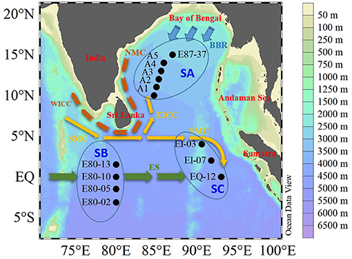
Figure 1. Sampling map and schematic diagram of the primary current regimes in the eastern Indian Ocean (EIO) in October and November 2020. Map created using Ocean Data View. The current systems included are the Bay of Bengal Runoffs (BBR), Northeast Monsoon Current (NMC), West Indian Coastal Current (WICC), East Indian Coastal Current (EICC), and Equatorial Streams (ES) (see Wei et al., 2019a; Guo et al., 2021). Stations A1, A2, A3, A4, A5, and E87-37 were defined as the SA area. Stations E80-02, E80-05, E80-10, and E80-13 were defined as the SB area. Stations EI-03, EI-07, and EQ-12 were defined as the SC area.

Determination of Nutrients and Chl-a

For the nutrient analysis, the seawater samples were filtered through a 0.45-μm pore size cellulose acetate membrane and then immediately frozen (−20°C) until measurements could be made be in the laboratory. The dissolved inorganic phosphate, dissolved silicate, dissolved inorganic nitrogen, nitrate (NO₃-N), nitrite (NO₂-N), and ammonium (NH₄-N) in the filtered seawater samples were measured with a Technicon AA3 AutoAnalyzer (Bran + Luebbe, Norderstedt, Germany). The analytical methods were performed according to a study by Hansen and Koroleff (1999).

For the chlorophyll-a (Chl-a) analysis, the seawater samples were filtered through a 0.2-μm pore size GF/F glass fiber filter (Whatman Corp.) and then refrigerated at −20°C (no light) for further analysis in the laboratory. The Chl-a content was determined with a Turner-Designs Trilogy fluorometer (Sunnyvale, CA, USA) with reference to the method of Welschmeyer (1994).

For the chlorophyll fluorescence parameters produced by phytoplankton in the ocean, seawater samples from the upper euphotic depth (<200 m) were measured with FastOcean (Chelsea Technologies Group, Surrey, UK) according to the method described by Wei et al. (2019b). We calculated the maximum quantum yield of the photosystem II photochemistry in a dark-adapted state by referring to the study of Kitajima and Butler (1975) and expressed it as F_v/F_m, where F_v is the variable fluorescence and F_m is the maximum fluorescence.

Elemental Stoichiometry

A total organic carbon analyzer (Multi N/C TOC-3100; Jena, Germany) was used to determine DOC. We extracted the samples using pre-combusted (450°C for 6 h) GF/F glass fiber filters (25 mm in diameter) to assess the POC. Before being analyzed with a Costech Elemental Analyzer (ECS4010; Costech Analytical Technologies, Inc., Milan, Italy), the samples were acidified with 200 μl of 0.2 N HCl and dried overnight in an oven at 60°C.

Absorption Spectroscopy

A UV-visible spectrophotometer (TU-1810 DAPC; Beijing Persee General Instrument Co., Ltd., Beijing, China) with a 10-cm quartz cell was used to record absorption spectra from 200 to 800 nm. The absorption spectra were adjusted by subtracting the average absorption from 700 to 800 nm from ultrapure water (Milli-Q, Millipore, Billerica, MA, USA) as the blank. The absorption coefficient was calculated as a(λ) = 2.303A(λ)/l, where A(λ) is the absorbance at wavelength λ (nm) and l (m) represents the path length of the quartz cell. The CDOM concentration was quantified by the absorption coefficient at the 325-nm [a_cdm(325)] wavelength (Kowalczuk et al., 2010).

The EEM Spectra and PARAFAC Modeling

Three-dimensional EEM measurements were made with a fluorescence spectrophotometer (Hitachi F-7100; Tokyo, Japan). The voltage of the photomultiplier tube was set to 700 V. Fluorescence spectra detected the subsequent scanning of excitation (Ex) from 200 to 450 nm and emission (Em) from 250 to 550 nm. Excitation and Em slits were maintained at 5 nm, and the scanning speed was set at 1,200 nm/min. Instrument corrections were performed according to the instructions of the manufacturer. To eliminate the majority of the Raman scattering, we subjected each DOM spectrum to blank subtraction using ultrapure water (Milli-Q). The correction was followed by Raman calibration according to the literature (Lawaetz and Stedmon, 2009). A PARAFAC analysis was performed in Matlab 2018b (Mathworks, USA) with the DOMFluor toolbox. Every component model may be tested using a split-half analysis, residual analysis, and loadings to provide correct information about fluorescence components. Water Raman units were used to analyze all fluorescence data. Four fluorescence indices were derived from the EEMs: the FI (McKnight et al., 2001), the BIX (Parlanti et al., 2000), the HIX (Parlanti et al., 2000), and β/α (Parlanti et al., 2000).

Statistical Analysis

In this study, the correlations and plots of different hydrological parameters and CDOM-associated parameters were obtained with the ggplot2, corrplot, RColorBrewer, and reshape2 packages in RStudio. A confidence level of 95% was selected to strictly determine significance, and differences were considered significant at p < 0.05.

Results

Hydrological Parameters

The variation in temperature and salinity with depth in the three subregions is presented in Figure 2. The overall change in temperature, which decreased with increased depth, was similar in the three areas (Figure 2A). The temperatures of the SB (Space B, including stations E80-02, E80-05, E80-10, and E80-13) and SC (Space C, including stations EI-03, EI-07, and EQ-12) areas were higher than that of the SA area (Space C, including stations A1, A2, A3, A4, A5, and E87-37) at depths between 50 and 100 m. The salinity in all stations ranged from 31.891 to 35.277 (Figure 2B). The salinity in SA and SC generally increased with increased depth. The salinity in SB ranged from 34.758 to 35.277 (average salinity = 35.012). The salinity of the surface layer was generally lower in SA than in SB and SC (i.e., SA < SC < SB).

FIGURE 2

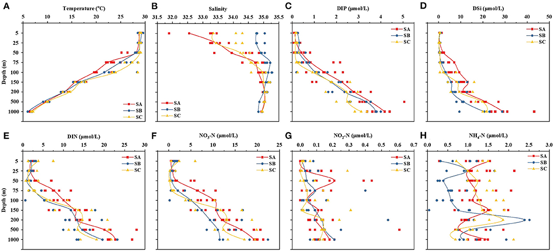
Figure 2. Variation in temperature, salinity, and nutrient concentrations at various depths (5–1,000 m) in the three subregions. The red, blue, and yellow lines represented the SA, SB, and SC areas, respectively.

Although the distribution of nutrients showed noticeable regional differences (Figures 2C–H), the lowest nutrient concentrations were invariably observed in the surface layer across all three regions. The concentration ranges of dissolved inorganic phosphate, dissolved silicate, dissolved inorganic nitrogen, NO₃-N, NO₂-N, and NH₄-N were 0.074 to 0.257, 0.111 to 1.454, 0.607 to 7.471, 0.186 to 5.971, 0 to 0.079, and 0.043 to 1.543 μmol/L in the surface layer (5 m), respectively (Figures 2C–H). In general, nutrient concentrations followed a depth gradient, with lower concentrations in the upper layers and higher ones in the bottom layers. The nutrient concentrations in SA were higher than those in SB and SC, especially in the 50–75 m layer. This reveals a potential replenishment of nutrients in the marginal waters of the Bay of Bengal, which could serve as a nutrient sink. Compared with SB and SC, higher Chl-a concentrations were found in the 50 m layer in SA. Photosynthesis is an important metabolic activity of phytoplankton, and the dimensionless number Fv/Fm is related to photosynthesis and hence productivity. As shown in Figure 3B, the trend for F_v/F_m was similar to that for Chl-a. This indicates that the influence of greater nutrients, the Bay of Bengal Runoffs, and the East Indian Coastal Current may promote activity among phytoplankton in SA.

FIGURE 3

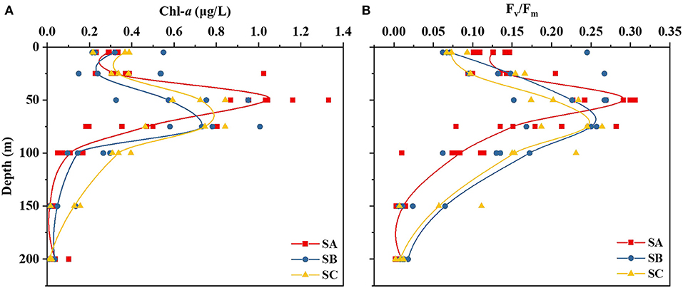
Figure 3. Variation in chlorophyll-a (Chl-a) and chlorophyll fluorescence (F_v/F_m) at various depths (5–1,000 m) in the three subregions. The red, blue, and yellow lines represented the SA, SB, and SC areas, respectively.

Distribution of DOC and POC Concentrations and Abundance of CDOM

Dissolved organic carbon and POC concentrations ranged from 0.025 to 1.285 and from 0.008 to 0.106 mg/L (Figures 4A,B), respectively, in all stations. In each subregion, DOC and POC concentrations decreased steadily with increased depth. For SA, the DOC and POC concentration ranges were 0.092–1.285 and 0.008–0.106 mg/L, respectively. For SB, they were 0.043–1.032 and 0.028–0.077 mg/L, respectively. For SC, they were 0.025–1.032 and 0.026–0.095 mg/L, respectively. The lowest value was found in the deep waters (1,000 m) of SA (0.008 mg/L, DOC), whereas the highest was in the surface layer of the Bay of Bengal, close to 200 nmi exclusive economic zone of Sri Lanka (station A1; 1.285 mg/L, POC). The abundance of CDOM was indicated by the index a_cdm(325). These a_cdm(325) values ranged from 0.011 to 0.161 for all seawater samples and increased with increasing depth (Figure 4C).

FIGURE 4

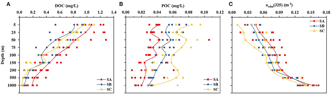
Figure 4. Variation in DOC and POC concentrations and the abundance of CDOM [a_cdm(325)] at various depths (5–1,000 m) in the three subregions. The red, blue, and yellow lines represented the SA, SB, and SC areas, respectively. DOC, dissolved organic carbon; POC, particulate organic carbon; CDOM, chromophoric DOM; a_cdm(325), an abundance of chromophoric dissolved organic matter.

Fluorescence Components

A total of 117 DOM samples collected from the three subregions of the EIO were modeled with PARAFAC. In addition, the spectral characteristics of all the components in this study were compared to those reported in earlier studies through an online repository of published PARAFAC components (Table 1). Four primary components were identified in SA (protein-, marine humic-, humic-, and tryptophan-like components) and SB (tryptophan-, humic-, and marine humic-like components), and three primary components were identified in SC (tryptophan-, marine humic-, and humic-like components) (Supplementary Figure 1 and Table 1). As shown in Figure 4, six independent components were identified by the PARAFAC analysis. Component 1 exhibited two fluorescence peaks centered at the Ex/Em wavelength pairs of 225/305 and 275/305 nm, respectively (Figure 5A). This component was identified as protein-like compounds (peak B), and its spectral characteristics were related to previous reports (Coble, 1996; Para et al., 2010). Component 2 was made up of two fluorescence peaks (Ex/Em wavelengths = 225/275 and 300–400 nm; Figure 5B), which we ascribed to tryptophan-like compounds (peak T) (Coble et al., 1998). Component 3 (Ex/Em = 260/458 nm) corresponded to humic-like fluorescence (peak C, Figure 5C) (Yamashita and Tanoue, 2008). Component 4 (Ex/Em = 235/400 nm) was distinguished as marine humic-like components (Figure 5D) (Yao et al., 2011). Components 5 and 6 (Ex/Em = 250/325 and 425 nm) were assigned to a humic-like component related to terrestrial substances (peak A; Figures 5E,F) (Stedmon et al., 2003; Yamashita et al., 2011).

TABLE 1

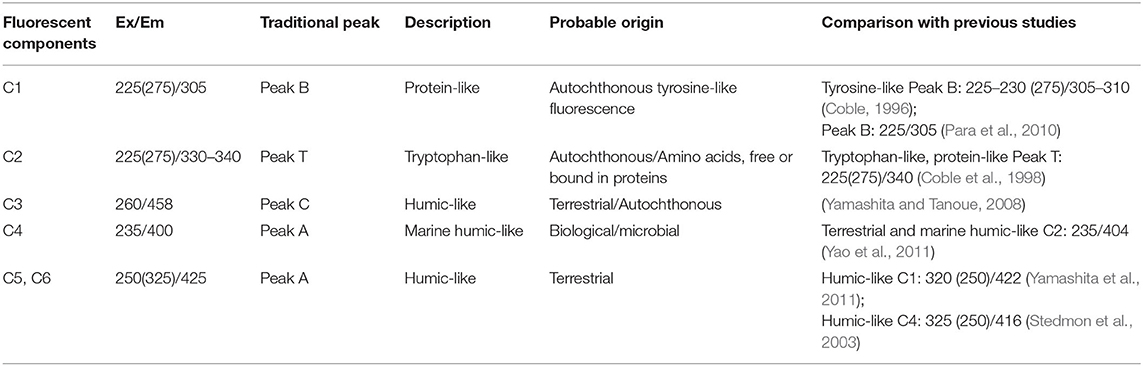
Table 1. Spectral characteristics of excitation and emission maxima of six fluorescence components identified by PARAFAC modeling compared with previously identified origins.

FIGURE 5

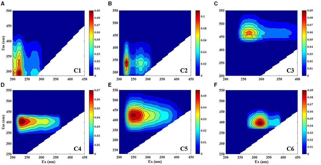
Figure 5. Excitation emission matrix (EEM) contour plots of the six fluorescence components identified by the parallel factor analysis (PARAFAC) model. C1–C6 represented components 1 to 6, respectively. The fluorescence intensity is given in Raman units (RU) with different scales.

The Depth Profiles of the CDOM FIs and Fluorescence Peaks

The fluorescence index is used to distinguish the origin of DOM. The FI values for the EIO samples ranged from 1.189 to 3.708 (Figure 6A). In particular, SA had a maximum FI value of 2.938 at 50 m, whereas SB and SC had maximum values of 2.709 and 2.819 at 150 m, respectively. From Figure 6B, we can see that BIX values decreased with increasing depth, from 1.661 to 0.893, with the lowest value recorded at 1,000 m in SA. The freshness index, β/α, (Parlanti et al., 2000; Huguet et al., 2009), in which the β peak represents recently created DOM whereas the α peak is older, more decomposed DOM, was also calculated. The β/α values of all samples were between 0.821 and 1.419. All samples with a β/α <1 were observed at depths of 1,000 m (Figure 6C). The HIX is an index of the degree of degradation in organic matter, with higher values being characteristic of higher molecular weight aromatic compounds (i.e., the HIX is directly proportional to the humic content of DOM) (Huguet et al., 2009). The degree of humification gradually intensified with increasing depth, especially in SA (Figure 6D).

FIGURE 6

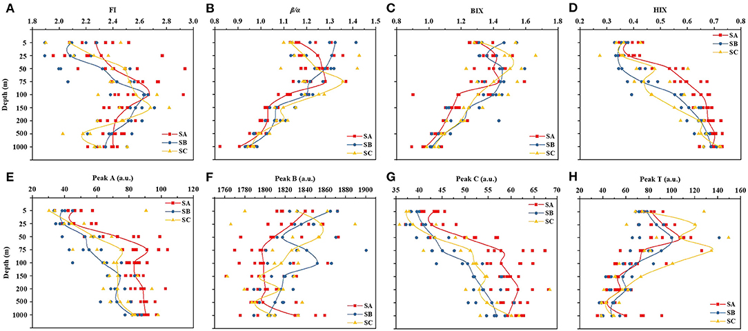
Figure 6. Variation in fluorescence indices (FI, BIX, β/α, and HIX) and peaks (peaks A, B, C, and T) at various depths (5–1,000 m) in the three subregions. The red, blue, and yellow lines represented the SA, SB, and SC areas, respectively. FI, fluorescence index; BIX, biological index; β/α, freshness index; HIX, humification index.

As can be seen in Figures 6E–H, the maximum fluorescence intensity recorded in the entire data set was 1900.5 (peak B), which had no obvious trend. Peaks A and C (protein-like) had the same trend in fluorescence intensity, which increased with increasing depth. Furthermore, SA values were commonly higher than SB and SC values. Peak T generally also decreased with increasing depth; the highest value for SC occurred at 50 m.

Discussion

Salinity and temperature have long been used in studies of the origin of marine waters. The above salinity and temperature data (Figures 2A,B) reveal that SA is a region of freshwater influence. Moreover, the saline surface seawaters carried by the eastward-flowing equatorial streams were obvious, especially in SB and SC. There is no difference in temperature among the three subregions, and relatively low salinity is influenced by freshwater flow and coastal currents (Unger et al., 2003; Shah et al., 2018). Sri Lanka is the center of an important commercial port. Most coastal waters are affected by pollution and eutrophication (Jiang et al., 2019; Rozemeijer et al., 2021). Simultaneously, SA is influenced by the East Indian Coastal Current and Bay of Bengal Runoffs, which has resulted in relatively rich nutrients that have made the area suitable for phytoplankton growth. This has caused an increase in the Chl-a concentration and F_v/F_m (Figures 2A,B).

By analyzing relevant hydrological parameters and spectroscopic indices, we found that most parameters were significantly positively or negatively correlated (Figure 7). Indeed, significant correlations were found between a_cdm(325) and other parameters. Furthermore, a_cdm(325) was positively correlated with depth, salinity, dissolved inorganic phosphate, dissolved silicate, dissolved inorganic nitrogen, NO₃-N, peak A, and peak C, and negatively correlated with temperature, β/α, Chl-a, F_v/F_m, DOC, POC, BIX, and peak T. These correlations suggest that CDOM might be used as a proxy for the marine DOM fraction (Coble, 2007). Moreover, in SA, we clearly saw that the FI, NO₂-N, and NH₄-N did not correlate significantly with the other parameters (Figure 7A). In contrast, in SB, the correlations between most parameters were significant, except for salinity, which had a weak correlation (Figure 7B). In SC, FI and NH₄-N did not correlate significantly with other parameters (Figure 7C). This further illustrates the significant differences in the correlations between hydrological parameters and spectroscopic indices in the three subregions of the EIO. Taken together, the differences in spatial and temporal distributions point to differences in multiple parameters.

FIGURE 7

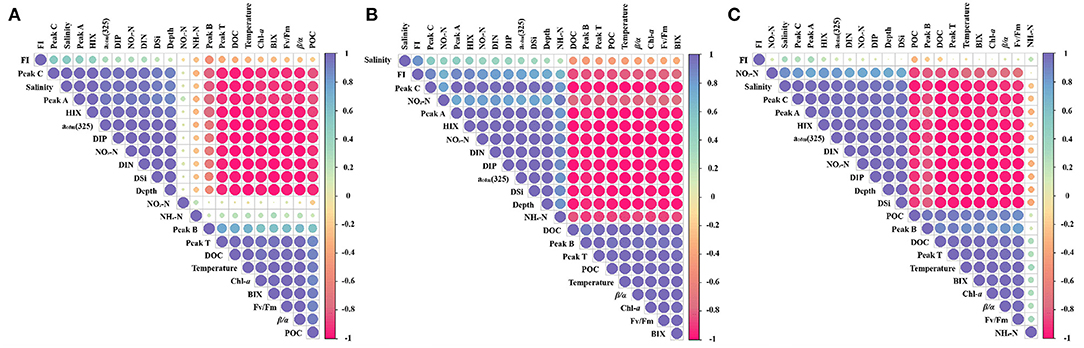
Figure 7. Correlation matrix among different hydrological parameters and CDOM-associated parameters of three subregions in the EIO. (A–C are represented as SA, SB, and SC areas) Only correlations with p < 0.05 are shown as circles and the color and the size of each circle indicate the correlation coefficient. The blue color indicates a positive correlation and the red color indicates a negative correlation.

DOC Accumulation and Export

We found that the concentration of DOC in the EIO decreased with increasing water depth (Figure 4A). Only a small amount of DOC was detected in the deeper layers. This trend is consistent with previous observations made throughout the oceans in the world (Hansell, 2002). It is now well-established from a variety of studies that DOC concentrations are typically greatest at the surface, drop quickly with depth, and then remain stable throughout the mesopelagic (200–1,000 m), bathypelagic (1,000–4,000 m), and abyssopelagic (4,000 m to bottom) layers (Hansell, 2002). These findings suggest that phytoplankton plays an important role in the production of DOC. In addition, phytoplankton decomposition creates huge volumes of degraded organic matter, which is then released into the ocean. In addition, DOC provides the carbon that microbes need to grow and function (Yang et al., 2018). Although bacteria are commonly thought to be the primary consumers of DOC, they may also generate DOC during cell division and virus lysis (Kawasaki and Benner, 2006).

The value of a_cdm(325) increased from the surface to the deep layers (Figure 4C), which is consistent with the range in oceanic CDOM concentrations reported in earlier research (Nelson and Siegel, 2013). In particular, surface depletion is consistent with severe photobleaching in surface waters caused by solar irradiation. This process results in a greater spectral slope and a considerable reduction in the abundance of CDOM (Li et al., 2019). In addition, oceanic CDOM can be produced during the remineralization of DOM by microorganisms (Nelson and Siegel, 2013; Hansman et al., 2015). The microbial metabolism resulting in the transformation of labile DOM into refractory DOM is likely responsible for the comparatively high abundance of CDOM we observed (Ortega-Retuerta et al., 2009).

The SA area is contained within the oxygen minimum zone. Thus far, previous studies have demonstrated that the production and degradation of organic matter are identical in oxic and anoxic environments (Lee, 1992). The decrease in free energy provided by the production and degradation of organic matter from aerobic to anaerobic respiration, resulting in lower community density and slower specific reactions, or not possible without O₂, could explain why the production and degradation of organic matter are slower and less efficient in marine environments under anoxic conditions (Fenchel and Finlay, 1995). Moreover, the primary productivity of phytoplankton and the generation of DOC are also affected by lower O₂ levels. One longitudinal study found that the optical characteristics of the anoxic layers in an oxygen minimum zone off the coast of Peru were distinct and dominated by marine humic-like compounds, indicating changes in chemical composition and a more refractory character of the DOC pool in anoxic waters (Loginova et al., 2016). This result was confirmed in our study, i.e., humic-like characteristics were more pronounced in the SA area than in the SB and SC areas (Figures 6D,E,G).

PARAFAC Components and Fluorescence Indices

To further understand the distribution of FDOM in the EIO, we built models with four to seven components, all of which we validated using a split-half analysis. Our seawater samples contained measurable concentrations of at least four fluorescence components, including commonly occurring protein- and humic-like components (Figure 5).

Four components (Components 3, 4, 5, and 6) (Figure 5) had previously been linked to high molecular weight and aromatic humic material referred to in the literature as peaks A and C (Stedmon et al., 2003; Yamashita and Tanoue, 2008; Yamashita et al., 2011; Yao et al., 2011; Table 1), and found in forest and wetland environments. These components are also more abundant in the open ocean. Autochthonous tryptophan-like substances, amino acids, and/or free or bound proteins are frequently linked with Component 2. As a result, it likely reflects the proteinaceous material generated by bacteria and phytoplankton in aquatic ecosystems. Component 1 (similar to peak B in the literature) was previously tentatively identified as autochthonous tyrosine-like fluorescence (Coble, 1996). Moreover, the presence of visible components (Components 1 and 2) might be explained by the suppression of tyrosine fluorescence through energy transfer to tryptophan and quenching by nearby groups (Lakowicz, 2013). Because the EIO is an oligotrophic marine region, there is greater photobleaching in the surface layer of the seawater, which may influence the peak position of microbial humic-like components. In addition, the absence of autochthonous or terrestrial inputs and poor biological or microbial production in the studied regions resulted in the low intensities of protein and humic-like components.

The vertical distributions of the index and peak intensity in our investigation are comparable to those of earlier ocean CDOM studies (Nelson and Siegel, 2013). In particular, there was evidence of the photobleaching of CDOM in surface waters and the microbial generation of CDOM in deeper waters (Nelson and Siegel, 2013). The parameters related to the fluorescence index and peak intensity showed significant variation by a depth that could be interpreted in terms of biogeochemical processing. The BIX can be used as an indicator of the traceability of DOM in aquatic ecosystems. Higher values indicate a greater degradation of DOM and the more likely production of endogenous carbon products. The trends in the BIX and β/α were similar (Figures 6B,C), i.e., a sharp decrease from 1.353 ± 0.101 (mean ± SD) and 1.213 ± 0.096 in the surface layer (5 m) to 1.016 ± 0.052 and 0.943 ± 0.042 in deep water (1,000 m), respectively. These trends reflect the fact that the amount of CDOM recently produced from a microbial activity is lower in deeper waters than in surface waters. The highest FI values were found at 50 m (Figure 3A). Moreover, the FI values were all >1.8, which indicates that the fluorescence component of DOM was mainly produced by microorganisms (Lavonen et al., 2015). In contrast with the BIX and β/α values, the HIX values gradually increased with depth (Figure 6D), which indicates a higher concentration of humus in deep waters (1,000 m), as humic substances accumulate in the deep ocean with the aging of water masses (Yamashita and Tanoue, 2008; Jørgensen et al., 2014).

In general, FDOM characteristics are related to environmental indicators and microbial activity (Williams et al., 2010). Peaks A and C can represent humus, which is similar to the trend in the HIX (Figures 6D,E,G). In contrast, peak T represents a protein, with a maximum at 75 m (Figure 6H). It has been reported in the literature that protein-like substances are less chemically stable and more easily degraded than tryptophan- and humic-like substances. Moreover, open-ocean fluorescence is generally low, with the highest fluorescence in the area of peak T. In other words, even the maximum fluorescence intensity is very low in the ocean. The global observations of altered fluorescence in the open ocean, which has been related to the remineralization of organic materials, might be explained by similar processes occurring in the open-ocean water column (Lechtenfeld et al., 2015).

Oceanic FDOM: Phytoplankton, Bacteria, or Remnant Terrestrial?

The CDOM samples we obtained from seawater samples produced protein-like fluorophores such as tyrosine- and tryptophan-like fluorescence that may be due to the natural assemblages of marine phytoplankton generating FDOM. Moreover, bacteria may generate secondary metabolites with complex molecular structures that render this material unnamable to further microbial degradation (Lechtenfeld et al., 2015). The structures that give DOM its fluorescence characteristics are created by a natural assemblage of marine microorganisms. Our findings indicate that phytoplankton have chemical characteristics comparable with those seen in terrestrial environments in which light and fluorescence can be absorbed. Regardless of the origin of DOM, microbial processing pathways can create a pool of varied compounds that tend to be durable in natural waters. This means that CDOM forming in the open ocean as a result of the biological pump can provide a semi-refractory material supply for the marine carbon cycle (Fakhraee et al., 2020).

A virtually continuous background signal has been seen in studies of CDOM absorption in the open ocean and has been interpreted as the potential residue of terrestrial biological components. Our findings show that terrestrial signals can be detected even when they are distant from recognized coastal impacts. Even when we confined data sets to seawater measurements acquired from at least 200 nmi away from any shore or island, we were able to determine the distinctive spectra of humic-like components (Components 3–6) in the EIO using PARAFAC. Low signal-to-noise ratios may have impacted these components, but they might also be photo-degraded refractory residues of the original terrestrial signal.

Conclusions

Numerous factors (e.g., physical, chemical, or biological factors) influence the composition and distribution of CDOM in the open sea. This study examined the hydrological parameters and properties of CDOM in the EIO. The fluorophore content, fluorescence indices, and fluorescence components allowed us to distinguish the overall origin and distribution of FDOM in the EIO. Different fluorescence components were identified by EEM-PARAFAC. Moreover, the FIs showed significant and meaningful variations in vertical distribution. This study was based on a limited number of samples and increasing the spatial coverage would help toward a more comprehensive understanding of the horizontal and vertical distribution of CDOM in the EIO.

Data Availability Statement

The raw data supporting the conclusions of this article will be made available by the authors, without undue reservation.

Author Contributions

JS and YL contributed to conception and design of the study. YL, XWa, XL, XWu, ZC, TG, WW, LY, YG, YW, GuoZ, and GuiZ organized the database. YL, XWa, YW, GuoZ, and GuiZ performed the statistical analysis. YL wrote the first draft of the manuscript. All authors contributed to manuscript revision, read, and approved the submitted version.

Funding

This research was financially supported by the National Natural Science Foundation of China (41876134) and the Changjiang Scholar Program of Chinese Ministry of Education (T2014253) to JS. Data and samples were collected onboard of R/V Shiyan-3 implementing the open research cruise NORC2020-10 supported by NSFC Ship time Sharing Project (project number: 41949910) and China-Sri Lanka Joint Center for Education and Research (Chinese Academy of Sciences).

Conflict of Interest

The authors declare that the research was conducted in the absence of any commercial or financial relationships that could be construed as a potential conflict of interest.

Publisher's Note

All claims expressed in this article are solely those of the authors and do not necessarily represent those of their affiliated organizations, or those of the publisher, the editors and the reviewers. Any product that may be evaluated in this article, or claim that may be made by its manufacturer, is not guaranteed or endorsed by the publisher.

Supplementary Material

The Supplementary Material for this article can be found online at: https://www.frontiersin.org/articles/10.3389/fmars.2021.742595/full#supplementary-material

References

Coble, P. G. (1996). Characterization of marine and terrestrial DOM in seawater using excitation-emission matrix spectroscopy. Marine Chem. 51, 325–346. doi: 10.1016/0304-4203(95)00062-3

CrossRef Full Text | Google Scholar

Coble, P. G. (2007). Marine optical biogeochemistry: the chemistry of ocean color. Chem. Rev. 107, 402–418. doi: 10.1021/cr050350+

PubMed Abstract | CrossRef Full Text | Google Scholar

Coble, P. G., Del Castillo, C. E., and Avril, B. (1998). Distribution and optical properties of CDOM in the Arabian Sea during the 1995 Southwest Monsoon. Deep Sea Res. 45, 2195–2223. doi: 10.1016/S0967-0645(98)00068-X

CrossRef Full Text | Google Scholar

Fakhraee, M., Planavsky, N. J., and Reinhard, C. T. (2020). The role of environmental factors in the long-term evolution of the marine biological pump. Nat. Geosci. 13, 812–816. doi: 10.1038/s41561-020-00660-6

CrossRef Full Text | Google Scholar

Fenchel, T., and Finlay, B. J. (1995). Ecology and Evolution in Anoxic Worlds. Oxford, NY: Oxford University Press.

Guo, C., Sun, J., Wang, X., Jian, S., Abu Noman, M., Huang, K., et al. (2021). Distribution and settling regime of Transparent Exopolymer Particles (TEP) potentially associated with bio-physical processes in the Eastern Indian Ocean. J. Geophys. Res. 126:e2020JG005934. doi: 10.1029/2020JG005934

CrossRef Full Text | Google Scholar

Hansell, D. A. (2002). “DOC in the global ocean carbon cycle,” in Biogeochemistry of Marine Dissolved Organic Matter, eds D. A. Hansell and C. A. Carlson (San Diego, CA: Academic Press), 685–715. doi: 10.1016/B978-012323841-2/50017-8

CrossRef Full Text | Google Scholar

Hansell, D. A., and Carlson, C. A., (eds.). (2014). Biogeochemistry of Marine Dissolved Organic Matter. London: Academic Press.

Hansen, H. P., and Koroleff, F. (1999). “Determination of nutrients,” in Methods of Seawater Analysis, eds K. Grasshoff, K. Kremling, and M. Ehrhardt (Wiley-VCH Verlag GmbH). doi: 10.1002/9783527613984.ch10

CrossRef Full Text | Google Scholar

Hansman, R. L., Dittmar, T., and Herndl, G. J. (2015). Conservation of dissolved organic matter molecular composition during mixing of the deep water masses of the northeast Atlantic Ocean. Mar. Chem. 177, 288–297. doi: 10.1016/j.marchem.2015.06.001

PubMed Abstract | CrossRef Full Text | Google Scholar

Holland, A., Stauber, J., Wood, C. M., Trenfield, M., and Jolley, D. F. (2018). Dissolved organic matter signatures vary between naturally acidic, circumneutral and groundwater-fed freshwaters in Australia. Water Res. 137, 184–192. doi: 10.1016/j.watres.2018.02.043

PubMed Abstract | CrossRef Full Text | Google Scholar

Huguet, A., Vacher, L., Relexans, S., Saubusse, S., Froidefond, J. M., and Parlanti, E. (2009). Properties of fluorescent dissolved organic matter in the Gironde Estuary. Org. Geochem. 40, 706–719. doi: 10.1016/j.orggeochem.2009.03.002

CrossRef Full Text | Google Scholar

Jiang, Q., He, J., Wu, J., Hu, X., Ye, G., and Christakos, G. (2019). Assessing the severe eutrophication status and spatial trend in the coastal waters of Zhejiang province (China). Limnol. Oceanogr. 64, 3–17. doi: 10.1002/lno.11013

CrossRef Full Text | Google Scholar

Jørgensen, L., Stedmon, C. A., Granskog, M. A., and Middelboe, M. (2014). Tracing the long-term microbial production of recalcitrant fluorescent dissolved organic matter in seawater. Geophys. Res. Lett. 41, 2481–2488. doi: 10.1002/2014GL059428

CrossRef Full Text | Google Scholar

Karl, D. M., Hebel, D. V., Björkman, K., and Letelier, R. M. (1998). The role of dissolved organic matter release in the productivity of the oligotrophic North Pacific Ocean. Limnol. Oceanogr. 43, 1270–1286. doi: 10.4319/lo.1998.43.6.1270

CrossRef Full Text | Google Scholar

Kawasaki, N., and Benner, R. (2006). Bacterial release of dissolved organic matter during cell growth and decline: molecular origin and composition. Limnol. Oceanogr. 51, 2170–2180. doi: 10.4319/lo.2006.51.5.2170

CrossRef Full Text | Google Scholar

Kitajima, M., and Butler, W. L. (1975). Quenching of chlorophyll fluorescence and primary photochemistry in chloroplasts by dibromothymoquinone. Biochim. Biophys. Acta 376, 105–115. doi: 10.1016/0005-2728(75)90209-1

PubMed Abstract | CrossRef Full Text | Google Scholar

Kowalczuk, P., Cooper, W. J., Durako, M. J., Kahn, A. E., Gonsior, M., and Young, H. (2010). Characterization of dissolved organic matter fluorescence in the South Atlantic Bight with use of PARAFAC model: Relationships between fluorescence and its components, absorption coefficients and organic carbon concentrations. Mar. Chem. 118, 22–36. doi: 10.1016/j.marchem.2009.10.002

CrossRef Full Text | Google Scholar

Lakowicz, J. R., (eds.). (2013). Principles of Fluorescence Spectroscopy. New York, NY: Springer Science and Business Media.

Lavonen, E. E., Kothawala, D. N., Tranvik, L. J., Gonsior, M., Schmitt-Kopplin, P., and Köhler, S. J. (2015). Tracking changes in the optical properties and molecular composition of dissolved organic matter during drinking water production. Water Res. 85, 286–294. doi: 10.1016/j.watres.2015.08.024

PubMed Abstract | CrossRef Full Text | Google Scholar

Lawaetz, A. J., and Stedmon, C. A. (2009). Fluorescence intensity calibration using the Raman scatter peak of water. Appl. Spectr. 63, 936–940. doi: 10.1366/000370209788964548

PubMed Abstract | CrossRef Full Text | Google Scholar

Lechtenfeld, O. J., Hertkorn, N., Shen, Y., Witt, M., and Benner, R. (2015). Marine sequestration of carbon in bacterial metabolites. Nat. Commun. 6, 1–8. doi: 10.1038/ncomms7711

PubMed Abstract | CrossRef Full Text | Google Scholar

Lee, C. (1992). Controls on organic carbon preservation: the use of stratified water bodies to compare intrinsic rates of decomposition in oxic and anoxic systems. Geochim. Cosmochim. Acta 56, 3323–3335. doi: 10.1016/0016-7037(92)90308-6

CrossRef Full Text | Google Scholar

Li, P., Tao, J., Lin, J., He, C., Shi, Q., Li, X., et al. (2019). Stratification of dissolved organic matter in the upper 2000 m water column at the Mariana Trench. Sci. Total Environ. 668, 1222–1231. doi: 10.1016/j.scitotenv.2019.03.094

PubMed Abstract | CrossRef Full Text | Google Scholar

Loginova, A. N., Thomsen, S., and Engel, A. (2016). Chromophoric and fluorescent dissolved organic matter in and above the oxygen minimum zone off Peru. J. Geophys. Res. 121, 7973–7990. doi: 10.1002/2016JC011906

CrossRef Full Text | Google Scholar

Lønborg, C., Álvarez-Salgado, X. A., Davidson, K., and Miller, A. E. (2009). Production of bioavailable and refractory dissolved organic matter by coastal heterotrophic microbial populations. Estuarine Coast. Shelf Sci. 82, 682–688. doi: 10.1016/j.ecss.2009.02.026

CrossRef Full Text | Google Scholar

Lønborg, C., Carreira, C., Jickells, T., and Álvarez-Salgado, X. A. (2020). Impacts of global change on ocean dissolved organic carbon (DOC) cycling. Front. Marine Sci. 7:466. doi: 10.3389/fmars.2020.00466

CrossRef Full Text | Google Scholar

McKnight, D. M., Boyer, E. W., Westerhoff, P. K., Doran, P. T., Kulbe, T., and Andersen, D. T. (2001). Spectrofluorometric characterization of dissolved organic matter for indication of precursor organic material and aromaticity. Limnol. Oceanogr. 46, 38–48. doi: 10.4319/lo.2001.46.1.0038

CrossRef Full Text | Google Scholar

Mopper, K., Kieber, D. J., and Stubbins, A. (2015). “Marine photochemistry of organic matter: processes and impacts,” in Biogeochemistry of Marine Dissolved Organic Matter, eds D. A. Hansell, and C. A. Carlson (Academic Press), 389–450. doi: 10.1016/B978-0-12-405940-5.00008-X

CrossRef Full Text | Google Scholar

Murphy, K. R., Timko, S. A., Gonsior, M., Powers, L. C., Wunsch, U. J., and Stedmon, C. A. (2018). Photochemistry illuminates ubiquitous organic matter fluorescence spectra. Environ. Sci. Technol. 52, 11243–11250. doi: 10.1021/acs.est.8b02648

PubMed Abstract | CrossRef Full Text | Google Scholar

Nelson, N. B., and Siegel, D. A. (2013). The global distribution and dynamics of chromophoric dissolved organic matter. Ann. Rev. Mar. Sci. 5, 447–476. doi: 10.1146/annurev-marine-120710-100751

PubMed Abstract | CrossRef Full Text | Google Scholar

Ortega-Retuerta, E., Frazer, T. K., Duarte, C. M., Ruiz-Halpern, S., Tovar-Sánchez, A., Arrieta, J. M., et al. (2009). Biogeneration of chromophoric dissolved organic matter by bacteria and krill in the Southern Ocean. Limnol. Oceanogr. 54, 1941–1950. doi: 10.4319/lo.2009.54.6.1941

CrossRef Full Text | Google Scholar

Para, J., Coble, P. G., Charrìère, B., Tedetti, M., Fontana, C., and Sempere, R. (2010). Fluorescence and absorption properties of chromophoric dissolved organic matter (CDOM) in coastal surface waters of the northwestern Mediterranean Sea, influence of the Rhône River. Biogeosciences 7, 4083–4103. doi: 10.5194/bg-7-4083-2010

CrossRef Full Text | Google Scholar

Parlanti, E., Wörz, K., Geoffroy, L., and Lamotte, M. (2000). Dissolved organic matter fluorescence spectroscopy as a tool to estimate biological activity in a coastal zone submitted to anthropogenic inputs. Org. Geochem. 31, 1765–1781. doi: 10.1016/S0146-6380(00)00124-8

CrossRef Full Text | Google Scholar

Paulmier, A., and Ruiz-Pino, D. (2009). Oxygen minimum zones (OMZs) in the modern ocean. Progr. Oceanogr. 80, 113–128. doi: 10.1016/j.pocean.2008.08.001

CrossRef Full Text | Google Scholar

Piketh, S. J., Tyson, P. D., and Steffen, W. (2000). Aeolian transport from southern Africa and iron fertilization of marine biota in the South Indian Ocean. South Afr. J. Sci. 96, 244–246.

Repeta, D. J. (2015). “Chemical characterization and cycling of dissolved organic matter,” in Biogeochemistry of Marine Dissolved Organic Matter, eds D. A. Hansell and C. A. Carlson (Boston, MA: Academic Press), 21–63. doi: 10.1016/B978-0-12-405940-5.00002-9

CrossRef Full Text | Google Scholar

Rozemeijer, J., Noordhuis, R., Ouwerkerk, K., Pires, M. D., Blauw, A., Hooijboer, A., et al. (2021). Climate variability effects on eutrophication of groundwater, lakes, rivers, and coastal waters in the Netherlands. Sci. Total Environ. 771:145366. doi: 10.1016/j.scitotenv.2021.145366

PubMed Abstract | CrossRef Full Text | Google Scholar

Shah, C., Sudheer, A. K., and Bhushan, R. (2018). Distribution of dissolved organic carbon in the Bay of Bengal: Influence of sediment discharge, fresh water flux, and productivity. Marine Chem. 203, 91–101. doi: 10.1016/j.marchem.2018.04.004

CrossRef Full Text | Google Scholar

Stedmon, C. A., Markager, S., and Bro, R. (2003). Tracing dissolved organic matter in aquatic environments using a new approach to fluorescence spectroscopy. Marine Chem. 82, 239–254. doi: 10.1016/S0304-4203(03)00072-0

CrossRef Full Text | Google Scholar

Thornton, D. C. O. (2014). Dissolved organic matter (DOM) release by phytoplankton in the contemporary and future ocean. Eur. J. Phycol. 49, 20–46. doi: 10.1080/09670262.2013.875596

CrossRef Full Text | Google Scholar

Unger, D., Ittekkot, V., Schäfer, P., Tiemann, J., and Reschke, S. (2003). Seasonality and interannual variability of particle fluxes to the deep Bay of Bengal: influence of riverine input and oceanographic processes. Deep Sea Res. 50, 897–923. doi: 10.1016/S0967-0645(02)00612-4

CrossRef Full Text | Google Scholar

Wei, Y., Zhang, G., Chen, J., Wang, J., Ding, C., Zhang, X., et al. (2019a). Dynamic responses of picophytoplankton to physicochemical variation in the eastern Indian Ocean. Ecol. Evol. 9, 5003–5017. doi: 10.1002/ece3.5107

PubMed Abstract | CrossRef Full Text | Google Scholar

Wei, Y., Zhao, X., Sun, J., and Liu, H. (2019b). Fast repetition rate fluorometry (FRRF) derived phytoplankton primary productivity in the Bay of Bengal. Front. Microbiol. 10:1164. doi: 10.3389/fmicb.2019.01164

PubMed Abstract | CrossRef Full Text | Google Scholar

Welschmeyer, N. A. (1994). Fluorometric analysis of chlorophyll a in the presence of chlorophyll b and pheopigments. Limnol. Oceanogr. 39, 1985–1992. doi: 10.4319/lo.1994.39.8.1985

CrossRef Full Text | Google Scholar

Williams, C. J., Yamashita, Y., Wilson, H. F., Jaffé, R., and Xenopoulos, M. A. (2010). Unraveling the role of land use and microbial activity in shaping dissolved organic matter characteristics in stream ecosystems. Limnol. Oceanogr. 55, 1159–1171. doi: 10.4319/lo.2010.55.3.1159

CrossRef Full Text | Google Scholar

Yamashita, Y., Panton, A., Mahaffey, C., and Jaff,é, R. (2011). Assessing the spatial and temporal variability of dissolved organic matter in Liverpool Bay using excitation–emission matrix fluorescence and parallel factor analysis. Ocean Dynamics 61, 569–579. doi: 10.1007/s10236-010-0365-4

CrossRef Full Text | Google Scholar

Yamashita, Y., and Tanoue, E. (2008). Production of bio-refractory fluorescent dissolved organic matter in the ocean interior. Nat. Geosci. 1, 579–582. doi: 10.1038/ngeo279

CrossRef Full Text | Google Scholar

Yang, J., Zhan, C., Li, Y., Zhou, D., Yu, Y., and Yu, J. (2018). Effect of salinity on soil respiration in relation to dissolved organic carbon and microbial characteristics of a wetland in the Liaohe River estuary, Northeast China. Sci. Total Environ. 642, 946–953. doi: 10.1016/j.scitotenv.2018.06.121

PubMed Abstract | CrossRef Full Text | Google Scholar

Yao, X., Zhang, Y., Zhu, G., Qin, B., Feng, L., Cai, L., et al. (2011). Resolving the variability of CDOM fluorescence to differentiate the sources and fate of DOM in Lake Taihu and its tributaries. Chemosphere 82, 145–155. doi: 10.1016/j.chemosphere.2010.10.049

PubMed Abstract | CrossRef Full Text | Google Scholar