Intrinsic and Wind-Driven Decadal Variability of the Kuroshio Extension in Altimeter Observations

Introduction

The Kuroshio Extension (KE) is an eastward extension to one of the most prominent western boundary currents of the global oceans – the Kuroshio. It is manifested in the maxima of horizontal sea surface height (SSH) gradient observed by satellite altimeters (Figure 1A, thin contours). Observational and modeling evidences have shown that the KE exhibits significant decadal bi-modal variability between a weak, southern, zonally contracted, unstable phase, and the phase of the opposite sign (Qiu and Chen, 2005, 2010; Qiu et al., 2007; Taguchi et al., 2007; Ceballos et al., 2009; Sugimoto and Hanawa, 2009; Kelly et al., 2010; Sugimoto et al., 2014). However, the mechanism for the decadal variability of the KE is not fully understood yet.

FIGURE 1

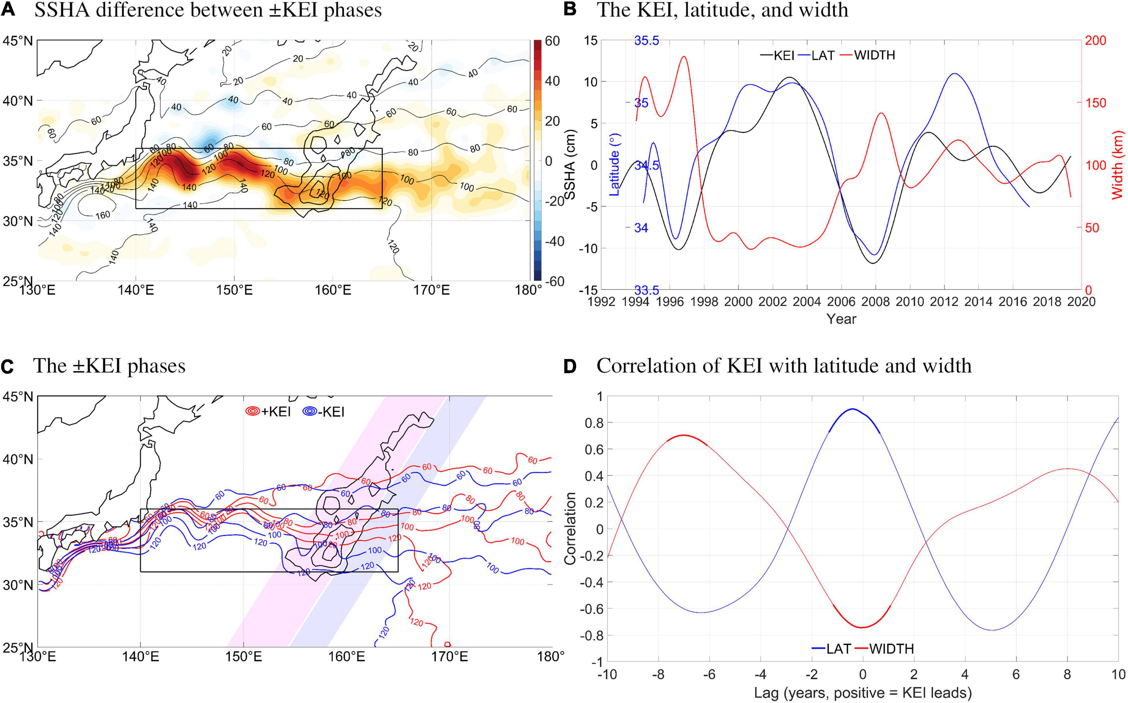
Figure 1. (A) Time-mean SSH (thin contours; cm) and bathymetry of the Shatsky Rise (thick contours; CI = 1 km starting from 5 km). Shading shows the SSHA difference (cm) between the ± KEI phases. (B) Time series of the KEI (black), latitude of the 100 cm SSH contour (142–160°E; blue), and meridional width between 90 and 110 cm SSH contours (red). (C) SSH (thin contours; cm) of the ± KEI phases. The Shatsky Rise is shown with thick contours as in (A). The magenta and blue patches will be used later in Figure 5. (D) Correlation between the KEI and the latitude and width indices. Thick curves denote statistical significance at the 95% level. The effective degrees of freedom are 2.6–4.4 (LAT) and 4.8–7.9 (WIDTH) depending on the lag.

FIGURE 2

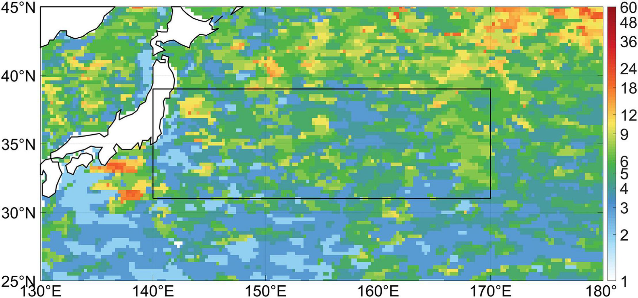
Figure 2. Decorrelation timescale (month) of the eddy field extracted by the 5° × 5° spatial filter.

FIGURE 3

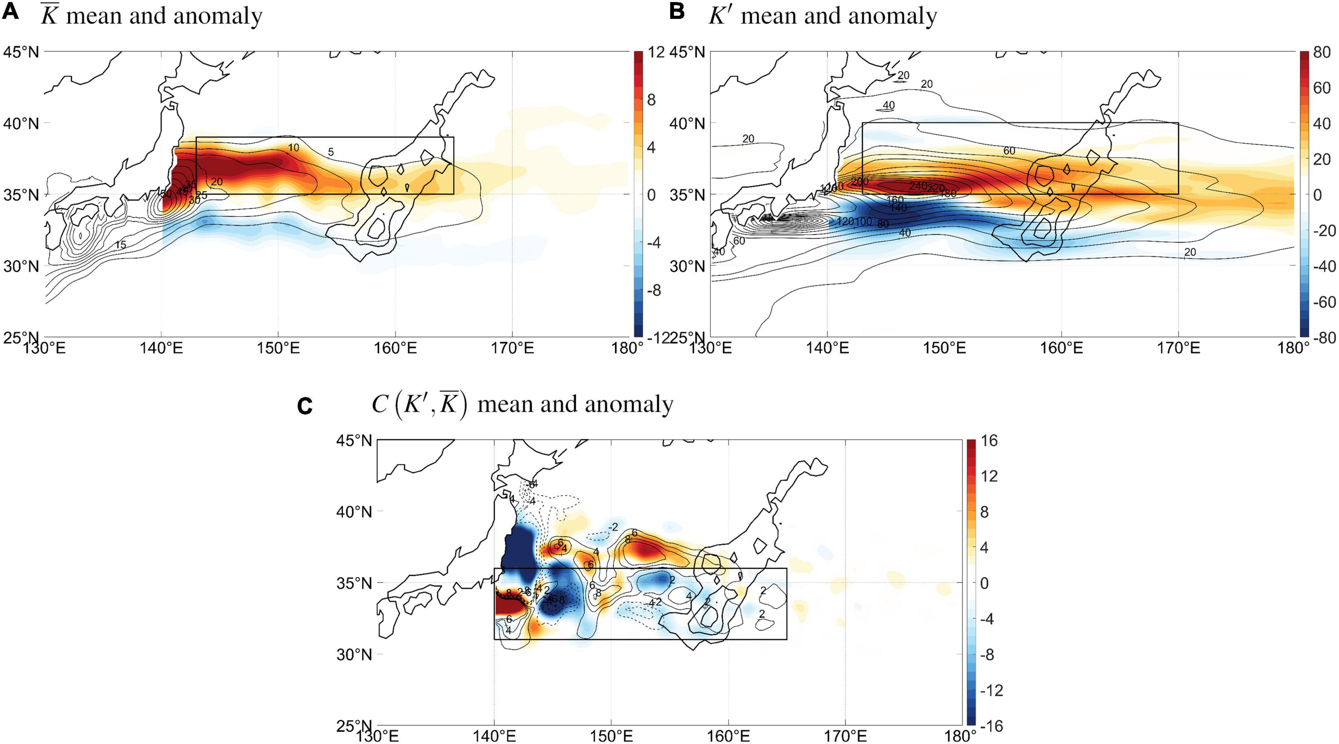
Figure 3. Time-mean (thin contours) and difference between the ± KEI phases (shading) for (A) mean-flow kinetic energy (J/m³), (B) eddy kinetic energy (J/m³), (C) eddy-to-mean-flow kinetic energy conversion rate $C(K^{\prime },\overline{K})$ (W/m³). Negative contours are dashed. Bathymetry of the Shatsky Rise is shown with the thick contours (CI = 1 km starting from 5 km).

FIGURE 4

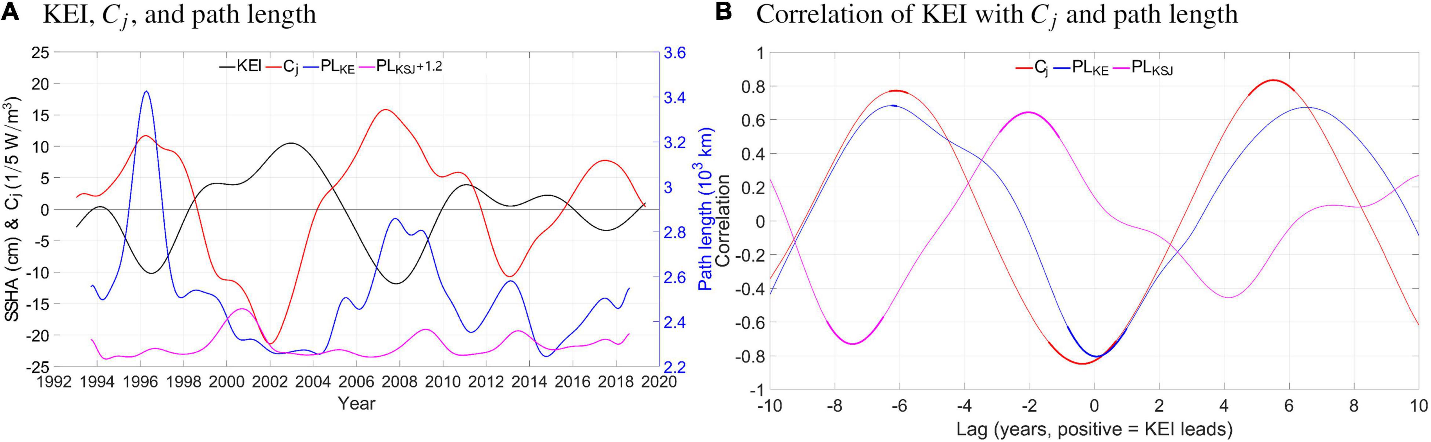
Figure 4. (A) Time series of the KEI (black, left axis; cm), along-jet eddy-to-jet conversion rate C_j averaged meridionally between 90 and 110 cm SSH contours between 142 and 160°E (red, left axis; 1/5 W/m³), and path length of the KE (blue, right axis; 10³ km) and KSJ (magenta, right axis; 10³ km) defined as the 100 cm SSH contour between 142 and 165°E and 133 and 143°E, respectively. (B) Correlation between the KEI and the C_j and path length indices in (A). Thick curves denote statistical significance at the 95% level. The effective degrees of freedom are 2.9–4.6 (C_j), 3.8–6.4 (PL_KE), and 6.5–10.8 (PL_KSJ) depending on the lag.

FIGURE 5

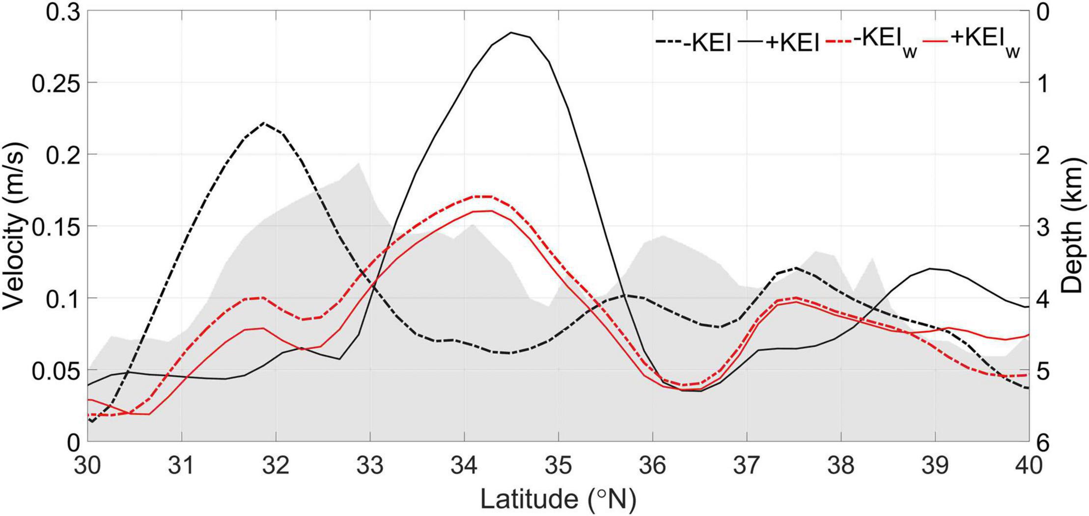
Figure 5. Geostrophic velocity of the KEI phases (black, left axis; m/s) zonally averaged across the blue patch in Figure 1C. Red curves are the same but for KEI_w phases. Gray shading shows zonally averaged bathymetry (right axis; km) across the magenta patch in Figure 1C.

Literature studies have identified two factors that are potentially important for maintaining the KE’s decadal variability, namely SSH anomaly (SSHA) driven by anomalous basin-scale wind stress curl and mesoscale eddy feedback. Particularly, early studies detected that decadal variability of the KE seems largely explained by propagation of baroclinic Rossby waves in response to wind-driven Ekman pumping in the central North Pacific (Miller et al., 1998; Deser et al., 1999; Xie et al., 2000; Seager et al., 2001; Qiu, 2002, 2003; Nonaka et al., 2006; Frankignoul et al., 2011). However, the wind-driven SSHAs can only explain broad-scale (≥1,000 km) SSHA variability, yet recent high-resolution satellite observations and modeling results revealed that the SSHAs in the KE region are actually narrowly confined (Taguchi et al., 2007; Sasaki and Schneider, 2011; Sasaki et al., 2013), and have much stronger amplitude (Qiu and Chen, 2005, 2010; Sasaki et al., 2013; Lin et al., 2014; Watanabe et al., 2016). On the other hand, recent studies noticed violent eddy generation in the vicinity of the KE jet due to the strong baroclinic instability (Ferrari and Wunsch, 2009; Bishop, 2013; Chen et al., 2014; Yang et al., 2018) and barotropic instability (Waterman et al., 2011; Waterman and Jayne, 2011; Yang and Liang, 2016; Yang et al., 2017; Ji et al., 2018), especially near the Shatsky Rise and Emperor Seamounts (Tanaka and Ikeda, 2004; Greene, 2010; Qiu and Chen, 2010; Lin et al., 2014). Recent findings reveal that mesoscale eddies can also feedback to the larger-scale jet through inverse energy cascade (Yang and Liang, 2016; Sérazin et al., 2018; Yang et al., 2018) and anomalous vorticity flux (Qiu and Chen, 2010; Delman et al., 2015). The exact role of eddy feedback in the decadal variation of the KE, however, is still poorly known.

Many literature studies attempted to address the problem of KE decadal variability by using either idealized (Dewar, 2003; Dijkstra and Ghil, 2005; Hogg et al., 2005; Pierini, 2006, 2010, 2011, 2014; Primeau and Newman, 2008; Zhang et al., 2017; Gentile et al., 2018) or full (Nonaka et al., 2006; Taguchi et al., 2007) numerical models. While the modeling approach is particularly useful in identifying potential mechanisms, it is subject to biases resulting from simplified or inaccurate model dynamics and limited resolution. Observation-based studies (Qiu and Chen, 2005, 2010; Lin et al., 2014; Qiu et al., 2014; Seo et al., 2014) typically rely on satellite altimeter measurements available since 1992, which are believed sufficient in resolving the mesoscale eddies and are now long enough for studying decadal variability of the KE.

Therefore, it is necessary to further investigate the mechanism of KE’s decadal variability, particularly regarding the respective roles of mesoscale eddies and wind-driven Rossby waves. Since three subjects (jet, eddy, and wind) are involved in this dynamic system, it is necessary to carefully identify and separate them from one another. This work attempts to examine the mechanism of the decadal variability of the KE using 27-year altimeter observations, with special attention on the jet-eddy energy transfer along the jet, and the separation of the wind-driven and intrinsic oceanic SSHAs. The rest of the paper is organized as follows: After introducing the observational data in section “Data,” section “Results” first analyzes the decadal variability of the jet and jet-eddy interaction, and then explores the relationship between the explicitly separated wind-driven and intrinsic SSHAs. The results are summarized in section “Summary and Discussion” followed by some discussions.

Data

We use the daily 1/4°-resolution satellite altimeter SSH product of AVISO (Ducet et al., 2000) for 1992–2019. Here the SSH is the absolute dynamic topography, which is the sum of the sea level anomaly and the mean dynamic topography, the latter of which is relative to the geoid. Sea surface heat and freshwater flux data from the NCEP/NCAR Reanalysis 1 dataset (Kistler et al., 2001) on a 2.5° grid are used to calculate the steric height variations (Supplementary Appendix A). Wind stress data also from NCEP/NCAR are employed in the 1.5-layer linear model to simulate the wind-driven SSH (Supplementary Appendix B). Observed and simulated SSH is averaged for each month, detrended, and applied a 4-year lowpass filter to remove interannual and shorter-term variabilities. Anomalies are defined as the deviation from the multi-year monthly climatology.

Results

Decadal Variability of the Kuroshio Extension and Role of Eddy

We follow Qiu et al. (2014) and define the SSHA averaged over the KE region (box in Figure 1A, 140–165°E, 31–36°N) as the KE index (KEI), which, as shown in Figure 1B (black curve), exhibits significant interannual to decadal variability. Positive and negative KEI events are then defined by a threshold of ±0.8 times standard deviation, and the composite-mean SSHAs are calculated, respectively, for the positive and negative KEI events. An alternative threshold of 1 times standard deviation does not change the results qualitatively. The positive-negative differences are shown in Figure 1A (shading). It is evident that the SSHA associated with the positive KEI is narrowly concentrated along the KE jet at 31–36°N, consistent with recent studies (Taguchi et al., 2007; Sasaki and Schneider, 2011; Sasaki et al., 2013). We then define the axis of the KE jet as the 100 cm SSH contour. The reason for choosing this contour level is based on Qiu and Chen (2005) who showed that the 170 cm SSH contour in their work is consistently located at the close vicinity of the maximum zonal geostrophic velocity and is thus a good index for the KE axis. Their SSH data is the sum of the sea level anomaly from the AVISO dataset and the mean dynamic topography given by Teague et al. (1990). The sea level anomaly is the same as in this work, but their mean dynamic topography is relative to 1,000 m below the sea surface, which is about 70 cm below our reference level, the geoid (not shown). Therefore, their 170 cm SSH contour is equivalent to the 100 cm contour here. The mean meridional width between the time-dependent 90 and 110 cm SSH contours is used as an (inverse) index of the strength of the jet in its core area. Apparently, the stronger the jet, the closer the contours, and hence the stronger the geostrophic velocity. This width/strength index, together with the latitude of the jet axis, is shown in Figure 1B (red and blue curves), which further demonstrates that comparing to the negative phase, the positive KEI features an enhanced and northward-shifted jet. This is also evident from the direct comparison between the KEI phases shown in Figure 1C, which reveals that the contours north of the jet axis do not move much (or even moved south as evident in the 60 cm contour), it is the jet axis itself and the contours south of it that are displaced northward, resulting in the thinning and strengthening. The cross-correlation between the strength and position indices shown in Figure 1D also suggests their close relationship, which can be understood in the framework of potential vorticity (PV) conservation: higher sea level to the south of the jet stretches the water column and the stronger jet enhances the anticyclonic relative vorticity, both requiring the planetary vorticity to increase. The KEI index, therefore, is representative of the integrated strength and position changes of the KE jet on decadal scales.

Next, we extract the large-scale component of the SSH using a 5° × 5° moving average filter and calculate the eddy component as the deviation from it. The use of a spatial filter instead of a canonical temporal one is justified by the decorrelation timescale of the resultant eddy field shown in Figure 2. East of 143°E, the decorrelation timescale has a median of 5 months and a 97-percentile of 10 months, confirming that the filter indeed does a good job in extracting the eddies. Eddies south of Japan extracted using such a moving average filter, however, are primarily manifested as the large meanders of the Kuroshio (Kawabe, 1995), which stand out in Figure 2 with decorrelation timescales of a few years. Since close to the coast the results of the moving average filter become questionable, in the following, eddy energetics analysis is only performed east of 142°E. Note that as in many previous studies (e.g., Qiu and Chen, 2005, 2010, 2013; Taguchi et al., 2007, 2010; Qiu et al., 2014, 2015, 2017, 2020; Yang and Liang, 2016, 2018; Yang et al., 2017, 2018; Nonaka et al., 2020), the extracted eddy field makes no strict distinction between mesoscale eddies and long baroclinic Rossby waves, since the two are both manifested as mesoscale SSH extrema and they often coincide and are in close dynamic association (Pingree and Sinha, 2001; Oliveira and Polito, 2013; Polito and Sato, 2015; Cheng et al., 2017).

Using u and v to denote the zonal and meridional component of the geostrophic velocity vector, surface kinetic energies are calculated for the mean-flow and eddies as,

$$\overline{K}=\frac{{\mathrm{\rho }}_0}{2}\left({\overline{u}}^2+{\overline{v}}^2\right)$$

$$K^{\prime }=\frac{{\mathrm{\rho }}_0}{2}\overline{u^{{}^{\prime }2}+v^{{}^{\prime }2}}$$

where overbar denotes the moving average filter, and prime denotes the eddy component, both defined above. ρ₀ = 1025 kg/m³ is a reference density. The kinetic energies are then averaged over the positive and negative KEI events and the difference between the phases is shown in Figures 3A,B. Both the mean-flow and eddy kinetic energies exhibit two bands on both sides of 35°N, representing a northward migration. Statistical significance of this result is confirmed by the high correlations (≥0.9) between the KEI and the energy terms averaged over the boxes indicated in the figures (not shown). Further, the kinetic energy conversion rate between the two components is calculated following von Storch et al. (2012):

$$C={\mathrm{\rho }}_0\left(\overline{u^{{}^{\prime }}{\mathbf{\text{u}}}^{{}^{\prime }}}\cdot \nabla \overline{u}+\overline{v^{{}^{\prime }}{\mathbf{\text{u}}}^{{}^{\prime }}}\cdot \nabla \overline{v}\right)$$

Positive C indicates eddy-to-jet conversion, and negative C indicates jet-to-eddy conversion. As shown by the contours in Figure 3C, climatologically, kinetic energy is mostly converted from eddies to the mean-flow (i.e., inverse cascade) downstream of 143°E, in agreement with literature studies (Yang and Liang, 2016; Sérazin et al., 2018; Yang et al., 2018). On the other hand, composite difference of the conversion rate (Figure 3C, shading) shows that with the positive KEI, the downstream inverse cascade exhibits a meridional dual pattern around 35°N indicating a meridional displacement along with the jet.

However, as the jet and the zone of high eddy activity migrate, it is better to study jet-eddy interaction following the core of the migrating jet (i.e., in the Lagrangian sense). To this end, we calculate the path length of the jet axis between 142 and 165°E as an index of along-jet eddy activity, since a convolved and longer axis indicates high eddy activity (e.g., Qiu and Chen, 2005, 2010; Qiu et al., 2014). The energy conversion rate C is then averaged over the area enclosed by the 90 and 110 cm SSH contours between 142 and 160°E as an indicator of jet-following energy conversion, denoted by C_j, the subscript j meaning “jet-following”. Such eddy activity and conversion indices are therefore quite different from what one may visually infer from Figures 3B,C at a fixed location (i.e., in the Eulerian sense). The resultant time series are shown in Figure 4A (red and blue curves). They are suggestive that on decadal timescales the eddy activity and the eddy-jet energy conversion at the jet core are in phase, both decreasing when the jet is stronger and northerly. Figure 4B confirms this and made clear the quasi-decadal periodicity of the indices.

These, however, are hard to interpret in a straightforward manner. When the jet is enhanced, forward energy cascade (i.e., negative C_j, or a reduction to the climatological inverse cascade) is expected to occur due to baroclinic instability (e.g., Ferrari and Wunsch, 2009; Bishop, 2013; Chen et al., 2014; Yang et al., 2018) and barotropic instability (e.g., Waterman et al., 2011; Waterman and Jayne, 2011; Yang and Liang, 2016; Yang et al., 2017; Ji et al., 2018), which is supported by Figure 3B. The forward cascade is then supposed to reinforce eddy activity. This process could be sketched with the following diagram:

$$\mathrm{jet}(+)\to {\mathrm{C}}_{\mathrm{j}}(-)\to \mathrm{eddy}(+)$$

Here “jet” means the integrated dynamic processes of the jet involving strength and position changes, as represented by the KEI index. The plus symbol indicates both the strengthening and the northward displacement. Positive correlation between jet and eddy, and negative correlation between C_j and eddy, are therefore expected, which are opposite to those found in Figure 4B at zero lag. It is also possible that the jet-eddy interaction is the other way around, i.e., driven by enhanced eddy activity and inverse cascade:

$$\mathrm{eddy}(+)\to {\mathrm{C}}_{\mathrm{j}}(+)\to \mathrm{jet}(+)$$

but in this case the jet-eddy and jet-C_j correlations are still of the wrong sign.

To tackle this problem, Qiu and Chen (2010) showed that with the Shatsky Rise being an important eddy generation site (Tanaka and Ikeda, 2004; Greene, 2010; Lin et al., 2014), a strong and northern jet axis would flow over a deep passage of the seamount at 35°N, resulting in reduced topographic interaction, which then causes weaker eddy activity and therefore reduced inverse cascade. The diagram of this regime is as follows:

$$\mathrm{jet}(+)\to \mathrm{topo}.\mathrm{inter}.(-)\to \mathrm{eddy}(-)\to {\mathrm{C}}_{\mathrm{j}}(-)$$

This argument is favored in this work, as Figure 5 (black curves) confirms the depth difference between the KEI phases, and the jet-eddy-C_j relationship agrees with Figure 4B. The initial impetus of the perturbation to the jet could be from the wind-driven SSHA anomalies (Qiu and Chen, 2010; Qiu et al., 2014) which is discussed in the next subsection. However, here we argue that the topography-mediated interaction pathway can also provide a feedback mechanism, forming a closed decadal cycle:

$$\mathrm{jet}(+)\to \mathrm{topo}.\mathrm{inter}.(-)\to \mathrm{eddy}(-)\to {\mathrm{C}}_{\mathrm{j}}(-)$$

$$\uparrow \mathit{\hspace{1em}\hspace{1em}\hspace{1em}\hspace{1em}\hspace{1em}\hspace{1em}\hspace{1em}\hspace{1em}\hspace{1em}\hspace{1em}\hspace{1em}\hspace{1em}\hspace{1em}\hspace{1em}\hspace{1em}\hspace{1em}\hspace{0.5em}\hspace{1em}}\downarrow$$

$${\mathrm{C}}_{\mathrm{j}}(+)\leftarrow \mathrm{eddy}(+)\leftarrow \mathrm{topo}.\mathrm{inter}.(+)\leftarrow \mathrm{jet}(-)$$

The key to this cycle is the C_j → jet positive correlation found in Figure 4B at lead time of 6 years by the C_j. The positive correlation when KEI leads and the negative peak at zero lag, on the other hand, are due to the decadal periodicity of the indices. More specifically, the C_j → jet process could be presumably attributed to eddies’ reinforcement to the southern recirculation gyre by means of anomalous vorticity forcing (Hurlburt et al., 1996; Qiu and Chen, 2010), and the strengthened recirculation gyre forces the jet northward while enhancing it. This highlights the role of inverse energy cascade in maintaining the decadal variability of the KE.

Moreover, another mechanism known as the intrinsic relaxation oscillation has been proposed based on idealized, barotropic, flat-bottom modeling results forced by climatological winds (Pierini, 2006; Gentile et al., 2018). This mechanism emphasizes the controlling role of the large meanders of the Kuroshio south of Japan (KSJ) on the KE jet. In a nutshell, it is argued that KSJ large meanders absorb anticyclonic PV advected from upstream and prevent it from feeding the KE, thus leading to the weakening of the KE in a few years. As the large meanders grow due to the accumulation of anticyclonic PV, they finally detach and turn into eddies. The KSJ, then, returns to a straight path, and the anticyclonic PV can therefore be advected to the recirculation gyre of the KE, both reinforcing the KE and at the same time spawning new large meanders to close the cycle. This paradigm solely depends on the relaxation oscillation of the gyre circulation, while jet-eddy and jet-topography interaction is not crucial.

We find here, however, that this mechanism seems missing in the real ocean. To show this, an index for the KSJ large meanders is constructed by the path length of the 100 cm SSH contour between 133 and 143°E (Figure 4A, magenta curve). Apparently, a meandering KSJ path must be convoluted and long. Cross-correlation of this KSJ index with the KEI (Figure 4B, magenta curve) exhibits strong and significant positive value when the KSJ leads by 2 years, but weak and insignificant at zero lag. This finding contradicts the argument of the relaxation oscillation theory that meandering KSJ leads to weakened KE in a few years. This is probably due to the lack of very large KSJ meanders in the satellite altimeter era. Traditionally, three typical states of the KSJ are defined after Kawabe (1985, 1995), i.e., the typical large meander (tLM), nearshore non-large meander (nNLM), and offshore non-large meander (oNLM) states as shown in Figure 6 (thin colorful curves). Since 1992, paths of the KSJ (thick and thin gray curves in the figure) are mostly in between the nNLM and oNLM states, while the tLM state only occurred once during winter 2004/2005 (Sugimoto and Hanawa, 2012; Seo et al., 2014). Our finding on KSJ path length – KEI concurrent relationship is in agreement with Sugimoto and Hanawa (2012) who concluded that the nNLM and tLM states are associated with stronger and more stable KE, while the oNLM and unclassified states are associated with the opposite. Knowing that the nNLM state exhibits the straightest KSJ path and the tLM the most convoluted, the fact that they are both associated to positive KEI thus nullifies the correspondence between KEI and the KSJ path.

FIGURE 6

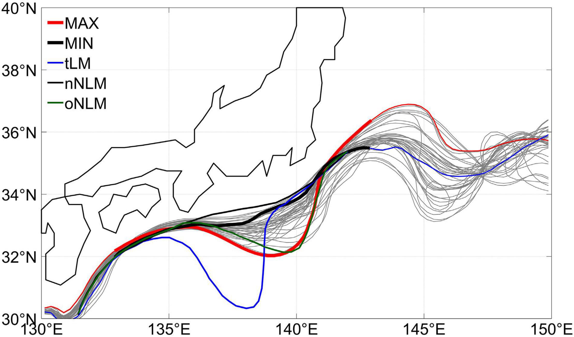
Figure 6. Paths of the 100 cm SSH contour in the KSJ region. Gray curves are snapshots 8 months apart. Thick curves are the overall shortest and longest paths. The three well-known typical states of the KSJ, i.e., the tLM, nNLM, and oNLM states defined conventionally by Kawabe (1985) are shown with thin colorful curves.

Wind-Driven and Intrinsic Variability

The next question is about the relationship of this oceanic intrinsic system with external forcing. Possible forcing factors include: (a) Steric height anomalies due to thermal expansion and saline contraction in response to the seasonally varying surface buoyancy fluxes (Stammer, 1997). They are estimated using air-sea heat and freshwater fluxes from the NCEP reanalysis as described in Supplementary Appendix A. (b) Westward propagating Rossby waves that originate at the eastern boundary, transited from coastally trapped Kelvin waves that travel northward from the tropics, not directly related to extratropical wind stress forcing. Supplementary Appendix A introduces the method to estimate the height anomalies associated with these waves. (c) Sea level anomalies due to Ekman pumping responses to wind stress curl forcing. These are originally the local SSH response to wind forcing at each location. After being generated, these SSH signals propagate westward both as barotropic Rossby waves which are very quick (Willebrand et al., 1980) and as baroclinic Rossby waves at much slower speed depending on the latitude (Chelton and Schlax, 1996; Killworth et al., 1997). Therefore, for a certain time and certain location, there are not only signals driven by local winds, but also those generated at remote locations in the east some time ago. Such SSHAs associated with local and remote wind-driven Rossby waves (termed SSHA_w) are calculated using a 1.5-layer reduced gravity model following Qiu (2003). The formulae and justification of this model are introduced in Supplementary Appendix B.

Next, we subtract the steric, eastern-boundary, and the local and remote wind-driven components of SSHA from the original SSHA, and refer to the residual wind-free part as the “intrinsic” component (SSHA_i) which is representative of the intrinsic oceanic jet-eddy dynamics. This linear approach is of course not fully accurate, yet the nonlinear interaction between the different types of sea level variations is presumably secondary. The wind-driven (KEI_w) and intrinsic (KEI_i) indices for the KE are then defined in the same manner as for the total KEI as box-averaged SSHA_w and SSHA_i in the KE region, and their time series are shown in Figure 7A. The reason why the time series before about 1999 are missing is because the calculation of SSHA_w requires sea level data a few years before, in order to account for the time needed for the Rossby waves generated near the eastern boundary to travel across the basin. Significant decadal-scale variability is evident for both the KEI_w and KEI_i.

FIGURE 7

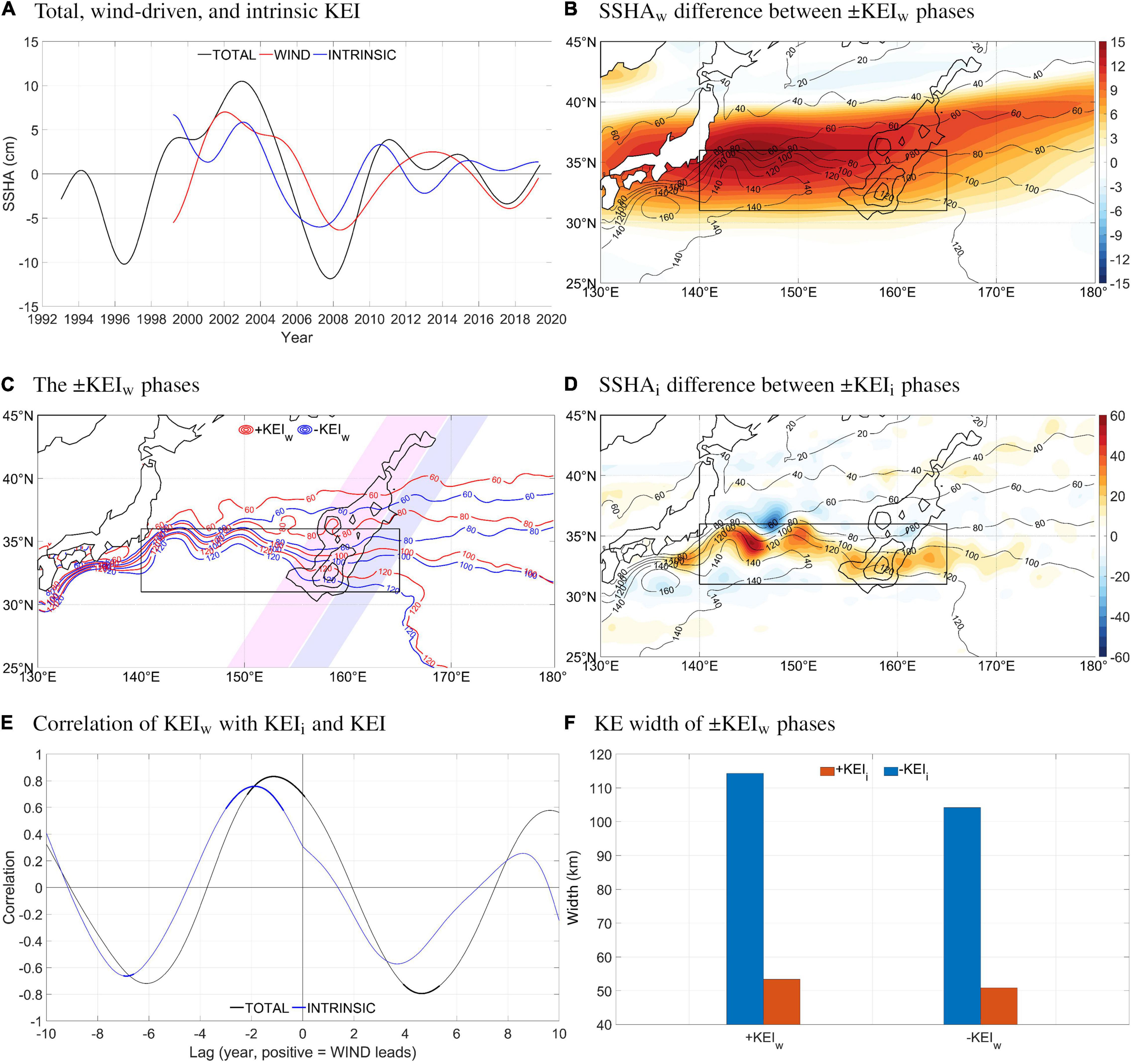
Figure 7. (A) Time series of total KEI, KEI_w, and KEI_i. (B) SSHA difference (shading; cm) between the ± KEI_w phases overlaid on time-mean SSH (thin contours; cm). (C) SSH (cm) of the ± KEI_w phases. (D) as (B), but for KEI_i. Note the different color scales in (B,D). (E) Correlation between KEI_w-KEI (black) and KEI_w-KEI_i (blue). Thick curves denote statistical significance at the 95% level. The effective degrees of freedom are 2.6–4.4 (TOTAL) and 4.8–7.9 (INTRINSIC) depending on the lag. (F) Bar chart of meridional distance between 90 and 110 cm SSH contours when the ± KEI_w phases are superimposed on the ± KEI_i phases. In (B–D), bathymetry of the Shatsky Rise is shown with the thick contours (CI = 1 km starting from 5 km).

Composite analysis is again performed to examine the SSHA_w associated with the KEI_w phases (Figures 7B,C). Comparing to the total SSHA, the SSHA_w is remarkably weaker (on the order of ∼1/5), and spans a much broader zonal and meridional range, consistent with earlier findings (e.g., Taguchi et al., 2007; Lin et al., 2014). Quantitatively, the strength and position changes of the jet across the KEI_w phases averaged over 142–160°E are, respectively, 4–19% and ∼1/3 of those associated with the total KEI. The percentages decrease dramatically downstream of Shatsky Rise (see also the red curves in Figure 5). On the other hand, the SSHA_i exhibits comparable magnitude and similar pattern as the total SSHA (Figure 7D). Therefore, it can be concluded that it is the intrinsic term, rather than the wind-driven part, that accounts for the majority of local SSHA variations in the KE region. However, it should be noted that area-averaged SSHA_w like the KEI_w can still explain a large fraction of the total SSHA thanks to its spatial broadness (KEI_w accounts for 64% of the variance of KEI). This is consistent with early studies using low-resolution observations and ocean models which argued that large-scale SSHA in the KE region can be adequately explained by wind-driven Rossby waves (e.g., Miller et al., 1998; Deser et al., 1999; Xie et al., 2000; Seager et al., 2001).

The relationship between the wind-driven and intrinsic SSHAs is explored based on the cross-correlation of the KEI_i and KEI_w indices shown in Figure 7E. It is found that the two are positively correlated when the KEI_i leads by 2 and 7 years. An insignificant negative correlation when the KEI_i lags by about 3 years is also visible. The concurrent correlation is positive but weak and insignificant. The physical causal relationship behind these statistical results is evaluated in the following.

First, for the intrinsic SSHAs to exert a forcing on the wind-driven counterpart, it must change the basin-scale wind stress. Previous studies have shown that frontal-scale SST anomalies associated with the decadal variability of the KE can indeed significantly modulate the overlying atmospheric storm track and basin-scale wind stress (Taguchi et al., 2009; Kwon et al., 2010; Frankignoul et al., 2011; O’Reilly et al., 2015; Révelard et al., 2016; Zhou et al., 2017; Zhang and Luo, 2017; Zhou, 2019; Zhou and Cheng, 2021). Qiu et al. (2014) used statistical methods to show that the positive KEI drives basin-scale wind stress anomalies that could further force negative SSHA_w response in about half a decadal cycle, in agreement with the negative correlation found at −7 years in Figure 7E of this work. Because the KEI switches sign at around year 5, which is 2 years before the arrival of the negative SSHA_w, the two would have positive correlation at lag −2, also consistent with the findings here. The feedback from the anomalous KE to wind-driven SSHA is thus favored in this work.

The positive concurrent correlation between KEI_w and KEI has often been regarded as an evidence to support the idea of wind-driven meridional displacement of the KE jet (e.g., Qiu and Chen, 2005, 2010; Taguchi et al., 2005, 2007; Qiu et al., 2014). We think, however, that this argument is questionable for three reasons. First, recalling Figures 5, 7C, the displacement caused by wind-driven SSHA is, in fact, minimal. Second, it is the correlation between KEI_w and KEI_i, instead of KEI, that should actually be investigated, which is much smaller and insignificant according to our results. Last, if this mechanism is true, the correlation between the two indices would maximize at zero lag, which is obviously not the case here. Therefore, the concurrent correlation is most likely merely a transition between the peaks on both sides as a result of the periodicity of the indices.

Finally, the negative correlation at positive lags suggests a possible mechanism of wind-triggered intrinsic oscillation at the delay of 3–4 years. Although statistical significance is low, it is still interesting to discuss the physical implications and relate to previous studies. One of the wind-triggered intrinsic oscillation mechanisms is proposed by Pierini and coauthors (Pierini, 2010, 2014; Zhang et al., 2017; Gentile et al., 2018) based on their idealized modeling results extending from the relaxation oscillation theory of Pierini (2006). Particularly, they argued that the intrinsic relaxation oscillation in the idealized model can be excited by SSHAs forced by either red-noise or nearly realistic winds, and that the negative SSHA_w south of the KE axis is the most effective trigger. However, as discussed in section “Decadal Variability of the Kuroshio Extension and Role of Eddy,” the intrinsic relaxation oscillation relies on a close association between the KE jet and the KSJ large meanders, which is not obvious in the altimeter era. It is therefore less promising to explain the delayed negative KEI_w-KEI_i correlation in the framework of the relaxation oscillation.

Here we propose another candidate mechanism. A closer look at Figure 7B reveals that the SSHA_w is not uniform in the meridional direction, having its maxima slightly to the north of the climatological KE jet at about 36°N. Therefore, contradicting common assumptions, the positive SSHA_w works to reduce the KE’s intensity (Figure 7F) while pushing it slightly poleward (Figure 7C). In fact, the positive SSHA_w in Figure 7B induces a clockwise secondary circulation that weakens the westerly current of the KE and KSJ. This leads to greater reduction to the KE in a few years because the weakened anticyclonic vorticity advection from upstream cannot balance the dissipation of vorticity due to the lateral eddy viscosity (Cessi et al., 1987; Pedlosky, 1987). The weakened KE jet migrates southward, encountering the shallower part of the Shatsky Rise and, thereby, evokes the intrinsic jet-eddy dynamical feedback. This mechanism is similar to the one suggested by Taguchi et al. (2005, 2007) based on the results of a general circulation model, except that they did not detect a delay between the wind-driven and intrinsic modes, and that they did not consider eddy feedback in the intrinsic mode. Together with the results of the last subsection, it could be concluded that the KE jet and eddy system maintains a closed feedback cycle that could be triggered by, and in pace with, the wind-forced SSHA, if the latter does play any role.

Summary and Discussion

In this study, we used the altimeter-observed sea surface height anomalies (SSHAs) to investigate the mechanism of the decadal variability of the Kuroshio Extension (KE). It is shown that the jet-eddy-topography feedback can maintain the decadal oscillation of the KE, in which inverse energy cascade is a key factor. The explicitly separated wind-driven and oceanic intrinsic SSHAs exhibit mutual forcing in both ways. On one hand, meridional displacement of the jet can force atmospheric storm track responses which, by means of anomalous wind stress forcing, further drive Rossby waves propagating from the eastern North Pacific. This results in negative correlation between the intrinsic and wind-driven components when the former leads by 7 years. On the other hand, the SSHAs associated with the wind-driven Rossby waves arrive at the KE region and change the velocity of the jet, which could evoke the intrinsic jet-eddy-topography feedback in about 3 years. The proposed relationship between jet, eddies, and wind-forced SSHAs is summarized schematically in Figure 8.

FIGURE 8

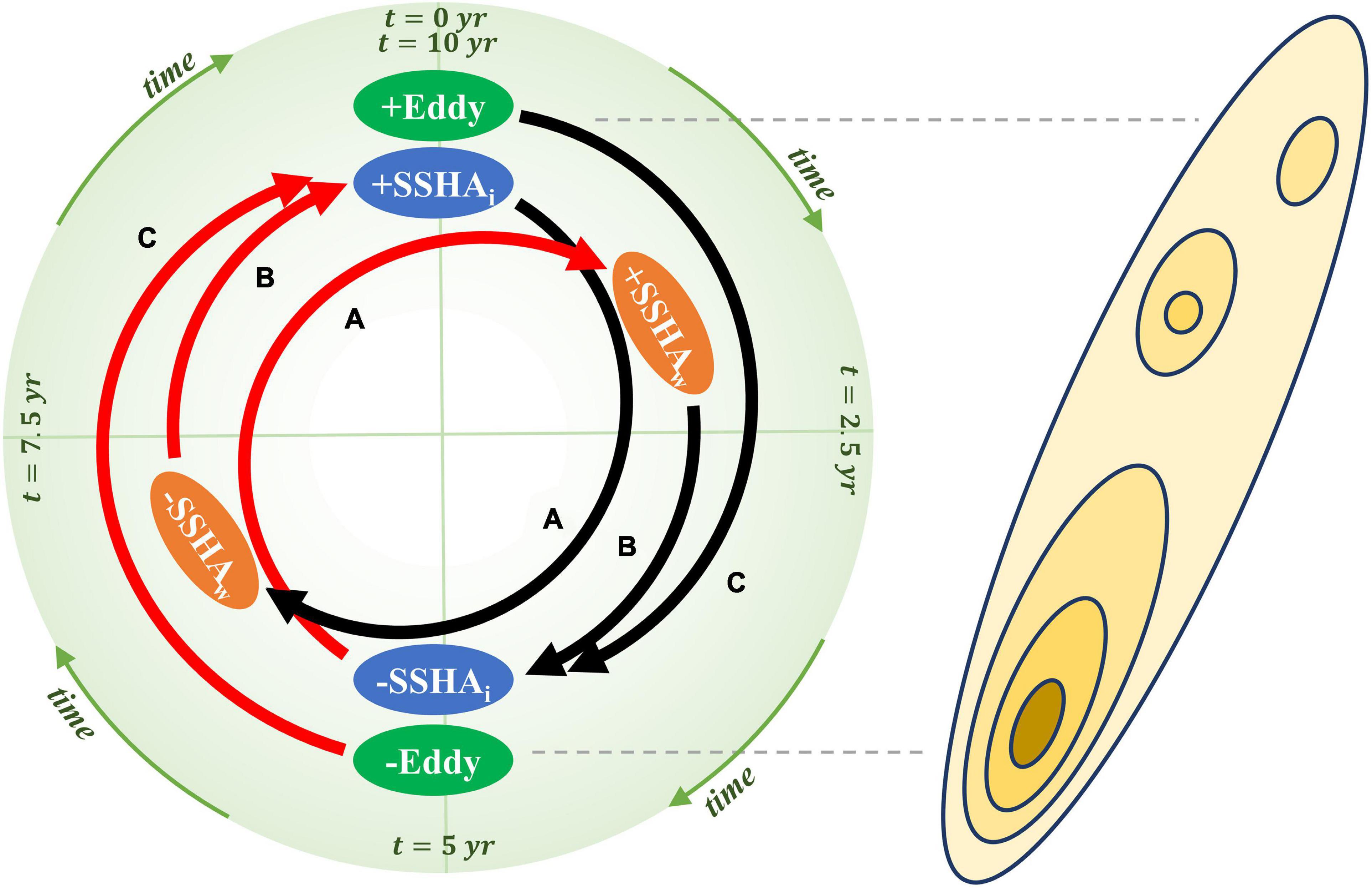
Figure 8. Sketch showing the decadal cycle of the intrinsic SSHA (SSHA_i), mesoscale eddies, and wind-driven SSHA (SSHA_w) with a diagram of the Shatsky Rise. Time evolves in the clockwise direction, and the thick arrows denote the (A) delayed modulation of wind-driven SSHA by intrinsic KE variability (B) delayed negative effect of wind-driven SSHA on the KE’s strength; (C) delayed energy feedback from eddies to the KE jet. The black and red colors indicate different polarities of the above feedbacks.

However, we must note that our results do not rule out the possibility that the relationship between the wind-driven and intrinsic variabilities is just a matter of coincidence, especially given the low statistical significance of such wind-triggered variability. While the wind-triggered mechanism proposed above is physically plausible, it is possible that the wind-driven SSHAs happen to lead the intrinsic cycle by 3–4 years. Recently, Nonaka et al. (2020) used ensemble modeling results to show that on the decadal timescale, the level of wind-driven variability of KE jet speed is 1.3 times that of the intrinsic counterpart. Their estimation method of the two components is statistical, based on a hypothesis that the ensemble mean represents the response to atmospheric forcing, while the ensemble spread is caused by ocean intrinsic processes. Their results, however, are subject to uncertainties due to model specificities and limited ensemble size (only 10). Further dynamical investigation with numerical models could be useful in validating the relative roles of the wind-driven and intrinsic components.

For future studies, it is also interesting to test the sensitivity of the KE to its relative position with the Shatsky Rise using numerical models, especially given the long-term migration of the KE axis in the context of climate change (e.g., Li et al., 2017). Since the atmospheric storm track and basin-scale wind stress undergo multi-decadal and climate change-related variations as well (Yin, 2005; Lu et al., 2010; Wu et al., 2011), models can be useful to assess the relationship between the wind-driven and intrinsic SSHAs beyond the time period studied in this article.

Data Availability Statement

The original contributions presented in the study are included in the article/Supplementary Material, further inquiries can be directed to the corresponding author.

Author Contributions

GZ performed most of the data analysis and wrote the initial manuscript. ZL contributed to the ideas behind the work, participated in the data analysis and visualization, and significantly improved the manuscript. XC participated in the discussions and improvement of the manuscript. All authors contributed to the article and approved the submitted version.

Funding

This work was supported by the National Natural Science Foundation of China (Grant No. 41906001), Natural Science Foundation of Jiangsu Province (Grant No. BK20190501), Fundamental Research Funds for the Central Universities (Grant Nos. B210202137 and B19020044), and the 2020 Jiangsu Shuangchuang (Mass Innovation and Entrepreneurship) Talent Program (Grant No. 2020-30448).

Conflict of Interest

The authors declare that the research was conducted in the absence of any commercial or financial relationships that could be construed as a potential conflict of interest.

Publisher’s Note

All claims expressed in this article are solely those of the authors and do not necessarily represent those of their affiliated organizations, or those of the publisher, the editors and the reviewers. Any product that may be evaluated in this article, or claim that may be made by its manufacturer, is not guaranteed or endorsed by the publisher.

Acknowledgments

The authors wish to thank Bo Qiu for the fruitful discussions. The AVISO altimeter observational data can be accessed under https://www.aviso.altimetry.fr. The NCEP/NCAR Reanalysis 1 is provided at https://www.esrl.noaa.gov/psd/data/gridded/data.ncep.reanalysis.html.

Supplementary Material

The Supplementary Material for this article can be found online at: https://www.frontiersin.org/articles/10.3389/fmars.2021.766226/full#supplementary-material

References

Bishop, S. P. (2013). Divergent eddy heat fluxes in the Kuroshio Extension at 144^°–148^°E. Part II: spatiotemporal variability. J. Phys. Oceanogr. 43, 2416–2431. doi: 10.1175/JPO-D-13-061.1

CrossRef Full Text | Google Scholar

Ceballos, L. I. Di Lorenzo, E., Hoyos, C. D., Schneider, N., and Taguchi, B. (2009). North Pacific gyre oscillation synchronizes climate fluctuations in the eastern and western boundary systems. J. Clim. 22, 5163–5174. doi: 10.1175/2009JCLI2848.1

CrossRef Full Text | Google Scholar

Cessi, P., Ierley, G., and Young, W. (1987). A model of the inertial recirculation driven by potential vorticity anomalies. J. Phys. Oceanogr. 17, 1640–1652. doi: 10.1175/1520-04851987017<1640:AMOTIR<2.0.CO;2

CrossRef Full Text | Google Scholar

Chelton, D. B., and Schlax, M. G. (1996). Global observations of oceanic Rossby waves. Science 272, 234L–238. doi: 10.1126/science.272.5259.234

CrossRef Full Text | Google Scholar

Chen, R., Flierl, G. R., and Wunsch, C. (2014). A description of local and nonlocal eddy–mean flow interaction in a global eddy-permitting state estimate. J. Phys. Oceanogr. 44, 2336–2352. doi: 10.1175/JPO-D-14-0009.1

CrossRef Full Text | Google Scholar

Cheng, X., McCreary, J. P., Qiu, B., Qi, Y., and Du, Y. (2017). Intraseasonal-to-semiannual variability of sea-surface height in the astern, equatorial Indian Ocean and southern Bay of Bengal. J. Geophys. Res. Oceans 122, 4051–4067. doi: 10.1002/2016JC012662

CrossRef Full Text | Google Scholar

Delman, A. S., McClean, J. L., Sprintall, J., Talley, L. D., Yulaeva, E., and Jayne, S. R. (2015). Effects of eddy vorticity forcing on the mean state of the Kuroshio Extension. J. Phys. Oceanogr. 45, 1356–1375. doi: 10.1175/JPO-D-13-0259.1

CrossRef Full Text | Google Scholar

Deser, C., Alexander, M. A., and Timlin, M. S. (1999). Evidence for a wind-driven intensification of the Kuroshio Current extension from the 1970s to the 1980s. J. Clim. 12, 1697–1706. doi: 10.1175/1520-04421999012<1697:EFAWDI<2.0.CO;2

CrossRef Full Text | Google Scholar

Dewar, W. K. (2003). Nonlinear midlatitude ocean adjustment. J. Phys. Oceanogr. 33, 1057–1082. doi: 10.1175/1520-04852003033<1057:NMOA<2.0.CO;2

CrossRef Full Text | Google Scholar

Dijkstra, H. A., and Ghil, M. (2005). Low-frequency variability of the large-scale ocean circulation: a dynamical systems approach. Rev. Geophys. 43:RG3002. doi: 10.1029/2002RG000122

CrossRef Full Text | Google Scholar

Ducet, N., Le Traon, P. Y., and Reverdin, G. (2000). Global high-resolution mapping of ocean circulation from TOPEX/Poseidon and ERS-1 and -2. J. Geophys. Res. Oceans 105, 19477–19498. doi: 10.1029/2000JC900063

CrossRef Full Text | Google Scholar

Ferrari, R., and Wunsch, C. (2009). Ocean circulation kinetic energy: reservoirs, sources, and sinks. Annu. Rev. Fluid Mech. 41, 253–282. doi: 10.1146/annurev.fluid.40.111406.102139

CrossRef Full Text | Google Scholar

Frankignoul, C., Sennéchael, N., Kwon, Y.-O., and Alexander, M. A. (2011). Influence of the meridional shifts of the Kuroshio and the Oyashio extensions on the atmospheric circulation. J. Clim. 24, 762–777. doi: 10.1175/2010JCLI3731.1

CrossRef Full Text | Google Scholar

Gentile, V., Pierini, S., de Ruggiero, P., and Pietranera, L. (2018). Ocean modelling and altimeter data reveal the possible occurrence of intrinsic low-frequency variability of the Kuroshio Extension. Ocean Model. 131, 24–39. doi: 10.1016/j.ocemod.2018.08.006

CrossRef Full Text | Google Scholar

Greene, A. D. (2010). Deep Variability in the Kuroshio Extension. Ph.D. thesis. Narragansett, RI: Graduate School of Oceanography, University of Rhode Island, 150.

Google Scholar

Hogg, A. M. C., Killworth, P. D., Blundell, J. R., and Dewar, W. K. (2005). Mechanisms of decadal variability of the wind-driven ocean circulation. J. Phys. Oceanogr. 35, 512–531. doi: 10.1175/JPO2687.1

CrossRef Full Text | Google Scholar

Hurlburt, H. E., Wallcraft, A. J., Schmitz, W. J., Hogan, P. J., and Metzger, E. J. (1996). Dynamics of the Kuroshio/Oyashio current system using eddy-resolving models of the North Pacific Ocean. J. Geophys. Res. Oceans 101, 941–976. doi: 10.1029/95JC01674

CrossRef Full Text | Google Scholar

Ji, J., Dong, C., Zhang, B., Liu, Y., Zou, B., King, G. P., et al. (2018). Oceanic eddy characteristics and generation mechanisms in the Kuroshio Extension region. J. Geophys. Res. Oceans 123, 8548–8567. doi: 10.1029/2018JC014196

CrossRef Full Text | Google Scholar

Kawabe, M. (1985). Sea level variations at the Izu Islands and typical stable paths of the Kuroshio. J. Oceanogr. Soc. Jpn. 41, 307–326. doi: 10.1007/BF02109238

CrossRef Full Text | Google Scholar

Kawabe, M. (1995). Variations of current path, velocity, and volume transport of the Kuroshio in relation with the large meander. J. Phys. Oceanogr. 25, 3103–3117. doi: 10.1175/1520-04851995025<3103:VOCPVA<2.0.CO;2

CrossRef Full Text | Google Scholar

Kelly, K. A., Small, R. J., Samelson, R. M., Qiu, B., Joyce, T. M., and Kwon, Y. O., et al. (2010). Western boundary currents and frontal air-sea interaction: gulf stream and kuroshio extension. J. Clim. 23, 5644–5667. doi: 10.1175/2010JCLI3346.1

CrossRef Full Text | Google Scholar

Killworth, P. D., Chelton, D. B., and de Szoeke, R. A. (1997). The speed of observed and theoretical long extratropical planetary waves. J. Phys. Oceanogr. 27, 1946–1966. doi: 10.1175/1520-04851997027<1946:TSOOAT<2.0.CO;2

CrossRef Full Text | Google Scholar

Kistler, R., Kalnay, E., Collins, W., Saha, S., White, G., and Woollen, J. (2001). The NCEP–NCAR 50–year reanalysis: monthly means CD–ROM and documentation. Bull. Am. Meteorol. Soc. 82, 247–267. doi: 10.1175/1520-04772001082<0247:TNNYRM<2.3.CO;2

CrossRef Full Text | Google Scholar

Kwon, Y.-O., Alexander, M. A., Bond, N. A., Frankignoul, C., Nakamura, H., Qiu, B., et al. (2010). Role of the gulf stream and Kuroshio–Oyashio systems in large-scale atmosphere–ocean interaction: a review. J. Clim. 23, 3249–3281. doi: 10.1175/2010JCLI3343.1

CrossRef Full Text | Google Scholar

Li, R., Jing, Z., Chen, Z., and Wu, L. (2017). Response of the Kuroshio Extension path state to near-term global warming in CMIP5 experiments with MIROC4h. J. Geophys. Res. Oceans 122, 2871–2883. doi: 10.1002/2016JC012468

CrossRef Full Text | Google Scholar

Lin, H., Thompson, K. R., and Hu, J. (2014). A frequency-dependent description of propagating sea level signals in the Kuroshio Extension region. J. Phys. Oceanogr. 44, 1614–1635. doi: 10.1175/JPO-D-13-0185.1

CrossRef Full Text | Google Scholar

Lu, J., Chen, G., and Frierson, D. M. W. (2010). The position of the midlatitude storm track and eddy-driven westerlies in aquaplanet AGCMs. J. Atmos. Sci. 67, 3984–4000. doi: 10.1175/2010JAS3477.1

CrossRef Full Text | Google Scholar

Miller, A. J., Cayan, D. R., and White, W. B. (1998). A westward-intensified decadal change in the North Pacific thermocline and gyre-scale circulation. J. Clim. 11, 3112–3127. doi: 10.1175/1520-04421998011<3112:AWIDCI<2.0.CO;2

CrossRef Full Text | Google Scholar

Nonaka, M., Nakamura, H., Tanimoto, Y., Kagimoto, T., and Sasaki, H. (2006). Decadal variability in the Kuroshio–Oyashio extension simulated in an eddy-resolving OGCM. J. Clim. 19, 1970–1989. doi: 10.1175/JCLI3793.1

CrossRef Full Text | Google Scholar

Nonaka, M., Sasaki, H., Taguchi, B., and Schneider, N. (2020). Atmospheric-driven and intrinsic interannual-to-decadal variability in the Kuroshio Extension jet and eddy activities. Front. Mar. Sci. 7:547442. doi: 10.3389/fmars.2020.547442

CrossRef Full Text | Google Scholar

Oliveira, F. S. C., and Polito, P. S. (2013). Characterization of westward propagating signals in the South Atlantic from altimeter and radiometer records. Remote Sens. Environ. 134, 367–376. doi: 10.1016/j.rse.2013.03.019

CrossRef Full Text | Google Scholar

O’Reilly, C. H., Czaja, A., O’Reilly, C. H., and Czaja, A. (2015). The response of the Pacific storm track and atmospheric circulation to Kuroshio Extension variability. Q. J. R. Meteorol. Soc. 141, 52–66. doi: 10.1002/qj.2334

CrossRef Full Text | Google Scholar

Pedlosky, J. (1987). Geophysical Fluid Dynamics, 2nd Edn. New York, NY: Springer New York, 710.

Google Scholar

Pierini, S. (2006). A Kuroshio Extension system model study: decadal chaotic self-sustained oscillations. J. Phys. Oceanogr. 36, 1605–1625. doi: 10.1175/JPO2931.1

CrossRef Full Text | Google Scholar

Pierini, S. (2010). Coherence resonance in a double-gyre model of the Kuroshio Extension. J. Phys. Oceanogr. 40, 238–248. doi: 10.1175/2009JPO4229.1

CrossRef Full Text | Google Scholar

Pierini, S. (2011). Low-frequency variability, coherence resonance, and phase selection in a low-order model of the wind-driven ocean circulation. J. Phys. Oceanogr. 41, 1585–1604. doi: 10.1175/JPO-D-10-05018.1

CrossRef Full Text | Google Scholar

Pierini, S. (2014). Kuroshio Extension bimodality and the North Pacific oscillation: a case of intrinsic variability paced by external forcing. J. Clim. 27, 448–454. doi: 10.1175/JCLI-D-13-00306.1

CrossRef Full Text | Google Scholar

Pingree, R., and Sinha, B. (2001). Westward moving waves or eddies (Storms) on the subtropical/azores front near 32^°N? Interpretation of the Eulerian currents and temperature records at moorings 155 (35.5^°W) and 156 (34.4^°W). J. Mar. Syst. 29, 239–276. doi: 10.1016/s0924-7963(01)00019-7

CrossRef Full Text | Google Scholar

Polito, P. S., and Sato, O. T. (2015). Do eddies ride on Rossby waves? J. Geophys. Res. Oceans 120, 5417–5435. doi: 10.1002/2015JC010737

CrossRef Full Text | Google Scholar

Primeau, F., and Newman, D. (2008). Elongation and contraction of the western boundary current extension in a shallow-water model: a bifurcation analysis. J. Phys. Oceanogr. 38, 1469–1485. doi: 10.1175/2007JPO3658.1

CrossRef Full Text | Google Scholar

Qiu, B. (2002). Large-scale variability in the midlatitude subtropical and subpolar North Pacific Ocean: observations and causes. J. Phys. Oceanogr. 32, 353–375. doi: 10.1175/1520-04852002032<0353:LSVITM<2.0.CO;2

CrossRef Full Text | Google Scholar

Qiu, B. (2003). Kuroshio Extension variability and forcing of the Pacific decadal oscillations: responses and potential feedback. J. Phys. Oceanogr. 33, 2465–2482. doi: 10.1175/2459.1

PubMed Abstract | CrossRef Full Text | Google Scholar

Qiu, B., and Chen, S. (2005). Variability of the Kuroshio Extension jet, recirculation gyre, and mesoscale eddies on decadal time scales. J. Phys. Oceanogr. 35, 2090–2103. doi: 10.1175/JPO2807.1

CrossRef Full Text | Google Scholar

Qiu, B., and Chen, S. (2010). Eddy-mean flow interaction in the decadally modulating Kuroshio Extension system. Deep Sea Res. 2 Top. Stud. Oceanogr. 57, 1098–1110. doi: 10.1016/j.dsr2.2008.11.036

CrossRef Full Text | Google Scholar

Qiu, B., and Chen, S. (2013). Concurrent decadal mesoscale eddy modulations in the western North Pacific subtropical gyre. J. Phys. Oceanogr. 43, 344–358. doi: 10.1175/JPO-D-12-0133.1

CrossRef Full Text | Google Scholar

Qiu, B., Chen, S., and Schneider, N. (2017). Dynamical links between the decadal variability of the Oyashio and Kuroshio Extensions. J. Clim. 30, 9591–9605. doi: 10.1175/JCLI-D-17-0397.1

CrossRef Full Text | Google Scholar

Qiu, B., Chen, S., Schneider, N., Oka, E., and Sugimoto, S. (2020). On reset of the wind-forced decadal Kuroshio Extension variability in late 2017. J. Clim. 33, 1–49. doi: 10.1175/JCLI-D-20-0237.1

CrossRef Full Text | Google Scholar

Qiu, B., Chen, S., Schneider, N., and Taguchi, B. (2014). A coupled decadal prediction of the dynamic state of the Kuroshio Extension system. J. Clim. 27, 1751–1764. doi: 10.1175/JCLI-D-13-00318.1

CrossRef Full Text | Google Scholar

Qiu, B., Chen, S., Wu, L., and Kida, S. (2015). Wind- versus eddy-forced regional sea level trends and variability in the North Pacific Ocean. J. Clim. 28, 1561–1577. doi: 10.1175/JCLI-D-14-00479.1

CrossRef Full Text | Google Scholar

Qiu, B., Schneider, N., and Chen, S. (2007). Coupled decadal variability in the North Pacific: an observationally constrained idealized model. J. Clim. 20, 3602–3620. doi: 10.1175/JCLI4190.1

CrossRef Full Text | Google Scholar

Révelard, A., Frankignoul, C., Sennéchael, N., Kwon, Y.-O., and Qiu, B. (2016). Influence of the decadal variability of the Kuroshio Extension on the atmospheric circulation in the cold season. J. Clim. 29, 2123–2144. doi: 10.1175/JCLI-D-15-0511.1

CrossRef Full Text | Google Scholar

Sasaki, Y. N., Minobe, S., and Schneider, N. (2013). Decadal response of the Kuroshio Extension jet to Rossby waves: observation and thin-jet theory*. J. Phys. Oceanogr. 43, 442–456. doi: 10.1175/JPO-D-12-096.1

CrossRef Full Text | Google Scholar

Sasaki, Y. N., and Schneider, N. (2011). Decadal shifts of the Kuroshio Extension jet: application of thin-jet theory*. J. Phys. Oceanogr. 41, 979–993. doi: 10.1175/2011JPO4550.1

CrossRef Full Text | Google Scholar

Seager, R., Kushnir, Y., Naik, N. H., Cane, M. A., and Miller, J. (2001). Wind-driven shifts in the latitude of the Kuroshio–Oyashio Extension and generation of SST anomalies on decadal timescales. J. Clim. 14, 4249–4265. doi: 10.1175/1520-04422001014<4249:WDSITL<2.0.CO;2

CrossRef Full Text | Google Scholar

Seo, Y., Sugimoto, S., and Hanawa, K. (2014). Long-term variations of the Kuroshio Extension path in winter: meridional movement and path state change. J. Clim. 27, 5929–5940. doi: 10.1175/JCLI-D-13-00641.1

CrossRef Full Text | Google Scholar

Sérazin, G., Penduff, T., Barnier, B., Molines, J.-M., Arbic, B. K., Müller, M., et al. (2018). Inverse cascades of kinetic energy as a source of intrinsic variability: a global OGCM study. J. Phys. Oceanogr. 48, 1385–1408. doi: 10.1175/JPO-D-17-0136.1

CrossRef Full Text | Google Scholar

Stammer, D. (1997). Steric and wind-induced changes in TOPEX/POSEIDON large-scale sea surface topography observations. J. Geophys. Res. Oceans 102, 20987–21009. doi: 10.1029/97JC01475

CrossRef Full Text | Google Scholar

Sugimoto, S., and Hanawa, K. (2009). Decadal and interdecadal variations of the aleutian low activity and their relation to upper oceanic variations over the North Pacific. J. Meteorol. Soc. Japan. Ser. II 87, 601–614. doi: 10.2151/jmsj.87.601

PubMed Abstract | CrossRef Full Text | Google Scholar

Sugimoto, S., and Hanawa, K. (2012). Relationship between the path of the Kuroshio in the south of Japan and the path of the Kuroshio Extension in the east. J. Oceanogr. 68, 219–225. doi: 10.1007/s10872-011-0089-1

CrossRef Full Text | Google Scholar

Sugimoto, S., Kobayashi, N., and Hanawa, K. (2014). Quasi-decadal variation in intensity of the western part of the winter subarctic sst front in the Western North Pacific: the influence of kuroshio extension path state. J. Phys. Oceanogr. 44, 2753–2762. doi: 10.1175/JPO-D-13-0265.1

CrossRef Full Text | Google Scholar

Taguchi, B., Nakamura, H., Nonaka, M., and Xie, S.-P. (2009). Influences of the Kuroshio/Oyashio Extensions on air–sea heat exchanges and storm-track activity as revealed in regional atmospheric model simulations for the 2003/04 cold season. J. Clim. 22, 6536–6560. doi: 10.1175/2009JCLI2910.1

CrossRef Full Text | Google Scholar

Taguchi, B., Qiu, B., Nonaka, M., Sasaki, H., Xie, S.-P., and Schneider, N. (2010). Decadal variability of the Kuroshio Extension: mesoscale eddies and recirculations. Ocean Dyn. 60, 673–691. doi: 10.1007/s10236-010-0295-1

CrossRef Full Text | Google Scholar

Taguchi, B., Xie, S.-P., Mitsudera, H., and Kubokawa, A. (2005). Response of the Kuroshio Extension to Rossby waves associated with the 1970s climate regime shift in a high-resolution ocean model. J. Clim. 18, 2979–2995. doi: 10.1175/JCLI3449.1

CrossRef Full Text | Google Scholar

Taguchi, B., Xie, S. P., Schneider, N., Nonaka, M., Sasaki, H., and Sasai, Y. (2007). Decadal variability of the Kuroshio Extension: observations and an eddy-resolving model hindcast. J. Clim. 20, 2357–2377. doi: 10.1175/JCLI4142.1

CrossRef Full Text | Google Scholar

Tanaka, K., and Ikeda, M. (2004). Propagation of Rossby waves over ridges excited by interannual wind forcing in a western North Pacific Model. J. Oceanogr. 60, 329–340. doi: 10.1023/B:JOCE.0000038339.21509.83

CrossRef Full Text | Google Scholar

Teague, W. J., Carron, M. J., and Hogan, P. J. (1990). A comparison between the generalized digital environmental model and Levitus climatologies. J. Geophys. Res. 95:7167. doi: 10.1029/JC095iC05p07167

CrossRef Full Text | Google Scholar

von Storch, J. S., Eden, C., Fast, I., Haak, H., Hernández-Deckers, D., Maier-Reimer, E., et al. (2012). An estimate of the Lorenz energy cycle for the World Ocean based on the 1/10^°STORM/NCEP simulation. J. Phys. Oceanogr. 42, 2185–2205. doi: 10.1175/JPO-D-12-079.1

CrossRef Full Text | Google Scholar

Watanabe, W. B., Polito, P. S., and da Silveira, I. C. A. (2016). Can a minimalist model of wind forced baroclinic Rossby waves produce reasonable results? Ocean Dyn. 66, 539–548. doi: 10.1007/s10236-016-0935-1

CrossRef Full Text | Google Scholar

Waterman, S., Hogg, N. G., and Jayne, S. R. (2011). Eddy–mean flow interaction in the Kuroshio Extension region. J. Phys. Oceanogr. 41, 1182–1208. doi: 10.1175/2010JPO4564.1

CrossRef Full Text | Google Scholar

Waterman, S., and Jayne, S. R. (2011). Eddy-mean flow interactions in the along-stream development of a western boundary current jet: an idealized model study. J. Phys. Oceanogr. 41, 682–707. doi: 10.1175/2010JPO4477.1

CrossRef Full Text | Google Scholar

Willebrand, J., Philander, S. G. H., and Pacanowski, R. C. (1980). The oceanic response to large-scale atmospheric disturbances. J. Phys. Oceanogr. 10, 411–429. doi: 10.1175/1520-04851980010<0411:TORTLS<2.0.CO;2

CrossRef Full Text | Google Scholar

Wu, Y., Ting, M., Seager, R., Huang, H.-P., and Cane, M. A. (2011). Changes in storm tracks and energy transports in a warmer climate simulated by the GFDL CM2.1 model. Clim. Dyn. 37, 53–72. doi: 10.1007/s00382-010-0776-4

CrossRef Full Text | Google Scholar

Xie, S.-P., Kunitani, T., Kubokawa, A., Nonaka, M., and Hosoda, S. (2000). Interdecadal thermocline variability in the North Pacific for 1958–97: a GCM simulation*. J. Phys. Oceanogr. 30, 2798–2813. doi: 10.1175/1520-04852000030<2798:ITVITN<2.0.CO;2

CrossRef Full Text | Google Scholar

Yang, H., Qiu, B., Chang, P., Wu, L., Wang, S., Chen, Z., et al. (2018). Decadal variability of eddy characteristics and energetics in the Kuroshio Extension: unstable versus stable states. J. Geophys. Res. Oceans 123, 6653–6669. doi: 10.1029/2018JC014081

CrossRef Full Text | Google Scholar

Yang, Y., and Liang, X. S. (2016). The instabilities and multiscale energetics underlying the mean–interannual–eddy interactions in the Kuroshio Extension region. J. Phys. Oceanogr. 46, 1477–1494. doi: 10.1175/JPO-D-15-0226.1

CrossRef Full Text | Google Scholar

Yang, Y., and Liang, X. S. (2018). On the seasonal eddy variability in the Kuroshio Extension. J. Phys. Oceanogr. 48, 1675–1689. doi: 10.1175/JPO-D-18-0058.1

CrossRef Full Text | Google Scholar

Yang, Y., Liang, X. S., Qiu, B., and Chen, S. (2017). On the decadal variability of the eddy kinetic energy in the Kuroshio Extension. J. Phys. Oceanogr. 47, 1169–1187. doi: 10.1175/JPO-D-16-0201.1

CrossRef Full Text | Google Scholar

Yin, J. H. (2005). A consistent poleward shift of the storm tracks in simulations of 21st century climate. Geophys. Res. Lett. 32:L18701. doi: 10.1029/2005GL023684

CrossRef Full Text | Google Scholar

Zhang, J., and Luo, D.-H. (2017). Impact of Kuroshio Extension dipole mode variability on the North Pacific storm track. Atmos. Ocean. Sci. Lett. 2834, 1–8. doi: 10.1080/16742834.2017.1351864

CrossRef Full Text | Google Scholar

Zhang, X., Mu, M., Wang, Q., and Pierini, S. (2017). Optimal precursors triggering the Kuroshio Extension state transition obtained by the conditional nonlinear optimal perturbation approach. Adv. Atmos. Sci. 34, 685–699. doi: 10.1007/s00376-017-6263-7

CrossRef Full Text | Google Scholar

Zhou, G. (2019). Atmospheric response to sea surface temperature anomalies in the mid-latitude oceans: a brief review. Atmos. Ocean 57, 319–328. doi: 10.1080/07055900.2019.1702499

CrossRef Full Text | Google Scholar

Zhou, G., and Cheng, X. (2021). Impacts of oceanic fronts and eddies in the Kuroshio-Oyashio Extension region on the atmospheric general circulation and storm track. Adv. Atmos. Sci. doi: 10.1007/s00376-021-0408-4 [Epub ahead of print].

CrossRef Full Text | Google Scholar

Zhou, G., Latif, M., Greatbatch, R. J., and Park, W. (2017). State dependence of atmospheric response to extratropical North Pacific SST anomalies. J. Clim. 30, 509–525. doi: 10.1175/JCLI-D-15-0672.1

CrossRef Full Text | Google Scholar