A space-time mosaic of seawater carbonate chemistry conditions in the north-shore Moorea coral reef system

1 Introduction

Warm water coral reef ecosystems are globally under severe threat from climate change driven stressors, such as ocean warming and ocean acidification (Hoegh-Guldberg, 1999; Kleypas et al., 1999a; Hughes et al., 2003; Hoegh-Guldberg et al., 2007; Pandolfi et al., 2011; Gattuso et al., 2015). These stressors are bound to increase as long as atmospheric CO₂ and global temperature are rising, making coral reefs among the most threatened ecosystems from global climate change (Knowlton, 2001; Knowlton and Jackson, 2008; Hughes et al., 2018; Bindoff et al., 2021). Given the large number of ecosystem services provided by coral reefs (Costanza et al., 1997; Costanza et al., 2017), especially their supporting of one of the highest levels of biodiversity in marine systems (Knowlton et al., 2010), the impairment of these systems will have substantial impact on global flora, fauna and human societies. Thus, preserving coral reefs against these stressors is a priority (Magnan et al., 2016), which requires a thorough understanding on how corals depend on and interact with their environment.

The local environmental conditions coral reefs experience can deviate substantially from those of the open ocean, especially for the seawater’s carbonate system parameters, such as dissolved inorganic carbon (DIC), total alkalinity (TA), pH (-log([H⁺])), the partial pressure of CO₂ (pCO₂), or the saturation state with respect to the mineral CaCO₃ aragonite, Ω_α (Manzello, 2010; Gray et al., 2012; Kealoha et al., 2017; Takeshita et al., 2018; Yan et al., 2018). This is a consequence of the interplay between coral metabolism altering the seawater chemistry in the overlying waters and the transport and mixing of the water across the reef (Anthony et al., 2011; Kleypas et al., 2011). Concretely, organic matter production by photosynthesis (by corals and algae) drives down seawater DIC and pCO₂, while keeping TA largely unchanged, and thus increasing pH and Ω_α (Sarmiento and Gruber, 2006). Respiration and remineralization of this organic matter, induces the opposite changes, with the net rate of organic matter production referred to as net community production (NCP). Calcification decreases DIC and TA (TA twice as much as DIC), thereby increasing pCO₂, and decreasing pH and Ω_α. The dissolution of the CaCO₃ induces the opposite changes, with the net rate of CaCO₃ formation being referred to as net community calcification (NCC). Thus, the net balance between NCP and NCC is a very critical determinant of how coral reef communities modulate the overlying seawater carbonate chemistry (c.f. Smith, 1973; Smith and Key, 1975; Suzuki and Kawahata, 1999; Suzuki and Kawahata, 2003; Cyronak et al., 2018), and affect the CO₂ source or sink behaviour of coral reefs. As pointed out by Suzuki and Kawahata (2003), reefs with a NCP to NCC production rate of less than about 0.6 (assuming both are positive) have a tendency to release CO₂ to the atmosphere, since the enhancing effect of NCC on pCO₂ exceeds the decreasing effect on pCO₂ by NCP.

The high metabolic rates and the often relatively slow transport of waters over the reefs system lead to both strong spatial gradients between the open ocean and these systems and high temporal variability. In fact, the variability of these parameters in coral reefs represents the strongest temporal variations in seawater chemistry observed anywhere in the world oceans (Hofmann et al., 2011). For example, the observed diel variability of pH in reef systems (Manzello, 2010; Gray et al., 2012; Price et al., 2012) tend to exceed the expected pH changes (~-0.4) over the next century even under a high CO₂ emission scenario (Orr et al., 2005; Feely et al., 2009; Bopp et al., 2013; Kwiatkowski et al., 2020). Similarly, the diel variations in seawater DIC and alkalinity within a reef can exceed 100 mmol m^-3 (Teneva et al., 2013; Albright et al., 2015) again several times larger than the anticipated changes under a high CO₂ emission scenario (~-10 to -25 mmol m^-3).

A good quantification and understanding of the spatio-temporal variations in the seawater’s chemistry in coral reefs are of interest for several reasons: First, the gradients in seawater carbonate chemistry parameters, such as DIC and TA, between the open ocean and the reef permit the quantification of NCP and NCC over the reef (Cyronak et al., 2018). Although such estimations depend sensitively on the spatio-temporal scale of the analysis (Takeshita et al., 2018), this approach has been used extensively since 1970s (Smith, 1973; Smith and Key, 1975; Gattuso et al., 1993; Gattuso et al., 1996; Watanabe et al., 2006; Shamberger et al., 2011; Kwiatkowski et al., 2016). Second, coral metabolism, and especially calcification with its high sensitivity to the saturation state of seawater Ω_α (Gattuso et al., 1998; Langdon and Atkinson, 2005; Kleypas and Yates, 2009; Kroeker et al., 2010; Kroeker et al., 2013), might vary within and between reefs in response to these differences in carbonate chemistry. Such variations in metabolic rates are especially relevant when assessing the impact of future ocean acidification on coral metabolism, since it is insufficient to assume that the corals experience the same changes in seawater chemistry as the open ocean (Andersson et al., 2014). Third, corals might have developed adaptive strategies to cope with these fluctuations in seawater carbonate chemistry (Boyd et al., 2016; Kroeker et al., 2020). This may permit them to cope better with the chemical changes that are lying ahead in a future high CO₂ ocean. Fourth, the mosaic of conditions within a coral reef ecosystem may lead to the emergence of biogeochemical niches, i.e., areas within the reef where biogeochemical conditions differ systematically in the mean and in their variance. Such niches could be relevant in two ways. On the one hand, these niches may facilitate the assessment of the acclimatization and adaptation potential of corals (Putnam, 2017). For instance, corals living in niches characterized with particularly low pH and aragonite saturation state may have adapted to such conditions (e.g. Fabricius et al., 2011; Bitter et al., 2019). On the other hand, such niches could also provide refugia (Manzello et al., 2012; Kapsenberg and Cyronak, 2019), i.e., regions within a reef that are less exposed to ocean acidification compared to other regions. Such ocean acidification refugia may offer means for managing coral ecosystems in a high CO₂ ocean.

With a few exceptions (e.g. Takeshita et al., 2018), the scale and resolution of the carbonate system measurements obtained so far in reef systems are inadequate to reveal the strong spatial and temporal gradients one can expect from the interplay between reef metabolism and reef circulation. As a result, our understanding of the spatio-temporal dynamics of seawater chemistry over coral reefs is rather limited. In particular, we do not know the degree to which the interaction can create distinct spatio-temporal patterns. This lack of understanding prevents us from assessing how variations in the carbonate chemistry can feed back to the coral’s metabolism or from determining whether biogeochemical niches emerge within the reef system. This lack also hinders the estimation of the potential resilience of corals against ocean acidification induced by the carbonate chemistry variations in the reef system.

Clearly, dedicated spatio-temporal surveys of the carbonate systems in and around coral reefs are urgently needed to fill this gap. But the large resources required to obtain such observations limit the scale and scope of this approach. A complimentary approach is the use of three-dimensional coupled hydrodynamic/coral reef ecosystem models, the first of which were developed only about a decade ago (Falter et al., 2013; Watanabe et al., 2013). These early studies tended to focus on the modeling of the flow of waters over the reef system and used prescribed fluxes of DIC and TA as a bottom boundary condition to represent the metabolic activity of the benthos. For instance, Falter et al. (2013) used their idealized setup to demonstrate how the magnitude of the diel variability in various biogeochemical properties scale with the forcing and geometry of the system and highlighted the critical role of reef flat geometry and bottom friction. Another thread was the development of models that incorporate detailed dynamics of the coral physiology (Nakamura et al., 2013) or of the coral-symbiont interactions (Baird et al., 2018). But these models were used in stand-alone applications, without explicit coupling to a hydrodynamic model. This changed when Nakamura et al. (2018) took coral reef ecosystem modeling efforts one step further by incorporating his coral physiology model into a hydrodynamic model to examine coral calcification under ocean acidification and sea level rise. But so far, this fully coupled model has not been used to investigate the spatio-temporal dynamics of the seawater’s chemistry overlying coral reef ecosystems and how this can give rise to distinct biogeochemical niches. This is the gap we aim to close with this study. To this end, we use a newly developed high-resolution three-dimensional hydrodynamic model coupled with a water column biogeochemistry module and a polyp photosynthesis/calcification model to investigate the interplay between the circulation, seawater carbonate chemistry and the activity of the corals with a focus on the spatio-temporal dynamics of the seawater chemistry. We configured this coupled model for the north-shore of Moorea Island, but it can be easily configured for any other tropical coral reef ecosystem.

2 Study area: Moorea island

Moorea Island is one of the French Polynesian islands located at 17°32’S, 149°50’W in the central South Pacific in close proximity to Tahiti. The coral reef system on the north-shore (Figure 1) is an ideal site for the investigation of the spatio-temporal variability in seawater chemistry driven by coral metabolism, owing to this system belonging to one of the best studied reef systems in the world (e.g. Gattuso et al., 1993; Gattuso et al., 1996; Frankignoulle et al., 1996; Anthony et al., 2011; Kleypas et al., 2011)

FIGURE 1

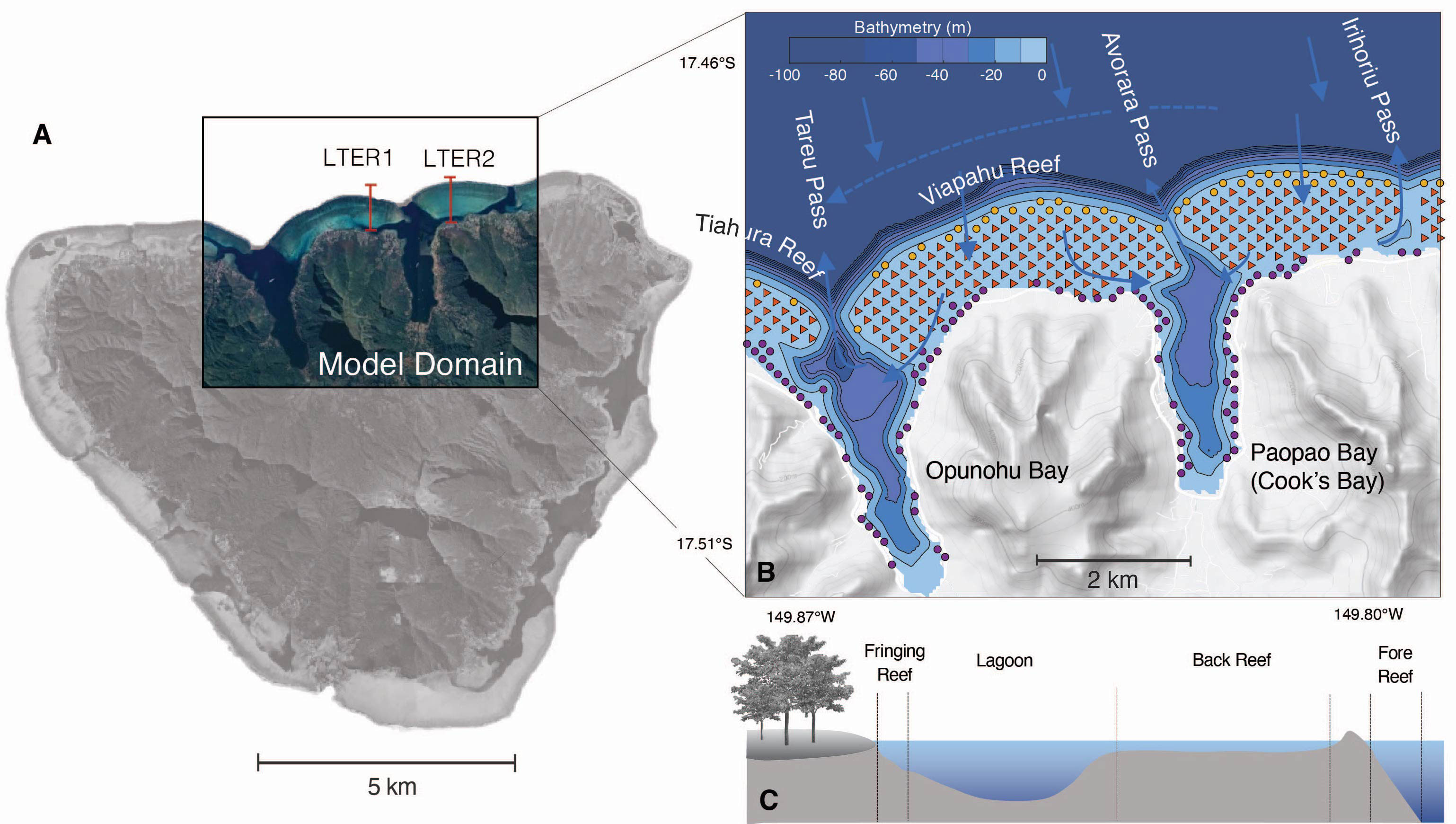
Figure 1 (A) Map view of Moorea island, showing the domain of the numerical model (colored inset) and the locations of the LTER1 and LTER2 stations of the Moorea LTER used in our study. (B) Map of the model domain showing the bathymetry (bluescale), the different reef types (fore reef: yellow circles, back reef: red triangles, and fringing reef: purple circles) and the names of the different bays, reefs, and passes. Also indicated with arrows is the typical circulation within and around the reef. (C) Schematic cross section across a typical reef showing the different reef types and the lagoon.

A barrier reef surrounds the island with a width of 0.5-1.5 km (Galzin and Pointier, 1985; Leichter et al., 2013). The north-shore coral reef system has a structure typical for many reef systems in the Pacific, consisting of a steeply sloping fore reef facing the ocean, a shallow back reef, and a fringing reef along the shorelines (Figure 1). The two relatively deep bays (Paopao (Cook’s) and Opunaho Bays in the east and west of our domain, respectively) are connected to the open ocean by narrow deep passes (Figure 1).

The flow over the reef is primarily governed by the breaking of surface waves, with tides and winds playing a minor role (Hench et al., 2008; Monismith et al., 2013). The small contribution of tides is largely a consequence of Moorea Island being located in an amphidromic point, resulting in small tidal amplitudes (< 30 cm). The breaking waves that arrive mostly from the north typically have a significant wave height of 1 to 2 m (Hench et al., 2008).

The pressure gradient set up by the breaking waves in the surf zone at the reef crest pushes the waters across the back reef and into the channels, working against the strong topographic drag induced by the roughness of the coral colonies (Symonds et al., 1995) (Figure 1). Most of the waters entering the bay from the channels tend to exit the bays rapidly through the passes in the form of narrow jets. With typical flow speeds over the back reef of about 0.1 m s^-1 (Hench and Rosman, 2013), the waters take a few hours to travel from the reef crest across the back reef to the channels. Typical residence times in the bays are a few hours to days (Herdman et al., 2015). When the waters exit the passes, they join an anti-cyclonic circulation that goes around the entire island, likely playing an important role in the retention of nutrients and organisms (Leichter et al., 2013).

The reefs of northern Moorea consist of coral aggregations separated by patches of sand and rubble. Other major benthic groups are crustose coralline algae, turf algae and macroalgae (Herdman et al., 2015). The corals of Moorea are predominantly branching corals of the families Pocilloporidae and Acroporidae, but also massive corals of the family Poritidae can be found. Although coral aggregations may reach to several meters in diameter, most of the colonies are relatively small (10 to 50 cm) due to the relatively frequent disturbances that occured over the past decades (Trapon et al., 2011). Since 1979, Moorea has been subject to nine coral bleaching events, two cyclones and two major outbreaks of the Crown of Thorns Starfish (COTS). The corals have shown a remarkable resilience, being able to recover relatively quickly after each of these major disturbances (Edmunds, 2020).

3 Materials and methods

3.1 Description of the model

To address our goals, we developed a fully coupled physical-biogeochemical-ecological model of the Moorea reef system (Figure 2). This model is based on our coupling of three existing models, i.e., the hydrodynamic model Coupled Ocean Atmosphere Wave and Sediment Transport (COAWST) Model (Warner et al., 2010), the Biogeochemical Elemental Cycling model (BEC) (Moore et al., 2004), and the coral polyp physiology model of (Nakamura et al., 2013) (Figure 2).

FIGURE 2

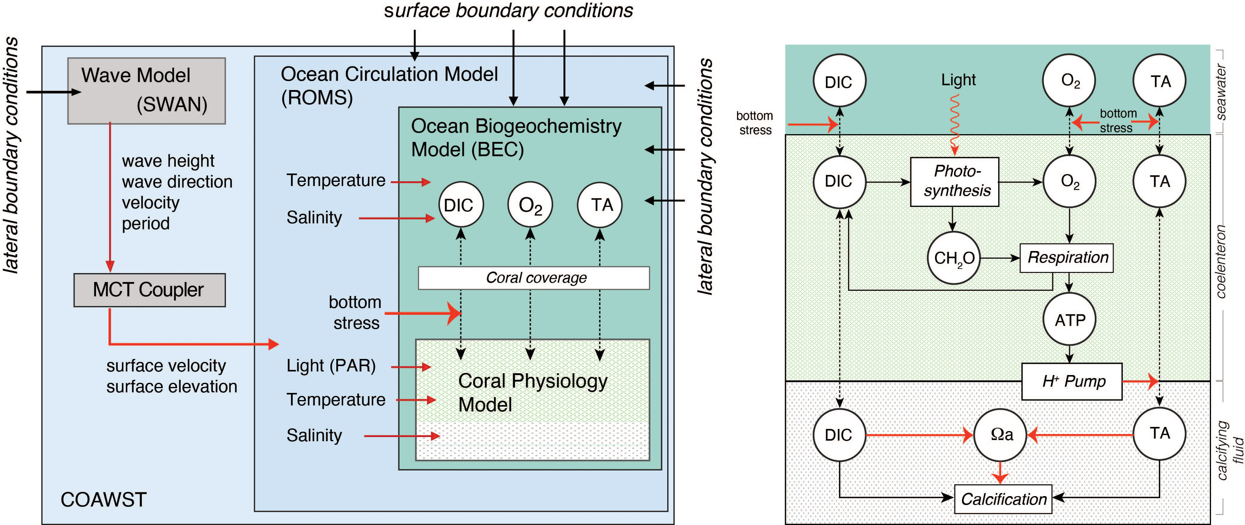
Figure 2 Diagrammatic depiction of the fully coupled physical-biogeochemical-ecological model of the Moorea North Shore Reef system. The model consists of four compartments, i.e., the wave model SWAN, the ocean circulation model ROMS, which are parts of COAWST, the ocean biogeochemical model BEC, and a coral physiology model (see text for details). Metabolic processes in the coral physiology model on the right hand side are shown in rectangles, while the considered state variables in each model are indicated in circles. Dashed lines indicate diffusive fluxes. Red arrows indicate controlling influences (e.g., the control of bottom stress on the diffusive exchange between corals and the seawater) or information transfer (e.g. the transfer of temperature and salinity from ROMS to BEC, or from ROMS to the coral physiology model).

The COAWST is a modeling system comprised of the Regional Ocean Modeling System (ROMS) (Shchepetkin and McWilliams, 2005) for the ocean, the Weather and Research Forecast (WRF) model for the atmosphere (Skamarock et al., 2005), the Simulation WAves Nearthshore (SWAN) model for the wave component (Booij et al., 1999), and the Community Sediment Transport Model for the sediment transport component (Warner et al., 2008), which exchange information through the Model Coupling Toolkit (MCT) coupler (Larson et al., 2005). In this study, we only use the ocean and the wave models, and force them with atmospheric and lateral boundary conditions. In this way, the three-dimensional reef scale circulation driven by the surface waves and buoyancy forcing are simulated.

BEC is a biogeochemical/ecological module that simulates the lower trophic level dynamics of pelagic marine ecosystem, as well as ocean biogeochemistry (Moore et al., 2004). In the context of this modeling study, we use BEC only to compute the inorganic biogeochemical processes in the seawater, especially the speciation of the carbonate system and the exchange of gaseous tracers (i.e., CO₂ and O₂) across the air-sea interface, while ROMS transports and mixes them across the domain. The reason for turning off the lower trophic levels in BEC is because the contribution of water column plankton to coral reef metabolism has been shown to be typically less than 1% (Delesalle et al., 1993).

The coral physiology model developed by Nakamura et al. (2013) represents the functioning of a single coral polyp and simulates, dependent on environmental conditions, photosynthesis by the symbiotic zooxhantellae, coral respiration, coral calcification, and other physiological processes occurring inside the corals (Figure 2). The fluxes of DIC, TA and O₂ between surrounding seawater and the upper seawater facing coral compartment, i.e., the coelenteron, is governed by the concentration gradient between the coelenteron and the seawater and by the mass transfer velocity that depends on the shear stress of the bottom currents (Hearn et al., 2001). The rate of photosynthesis (GPP) that occur in coelenteron depends on the available light (i.e., photosynthetically available radiation, PAR) and the concentration of bicarbonate (HCO₃^-) in this compartment. PAR is computed as a fixed fraction of the surface shortwave radiation in ROMS and provided as an input for the coral polyp model, while the bicarbonate concentration is computed from the concentration of DIC and TA in the coelenteron using the carbonate chemistry module mocsy 2.0 (Orr and Epitalon, 2015). Photosynthesis produces O₂ and carbohydrates CH₂O with a stoichiometric ratio of 1 to 1. Respiration (R), which also occurs in coelenteron, consumes CH₂O and O₂, produces DIC, and is controlled by the amount of carbohydrate and the concentration of O₂ within the coelenteron. The final process, i.e., calcification (G), which produces mineral CaCO₃ from DIC and TA, occur in the lower skeleton facing polyp compartment, i.e. calcifying fluid, and is controlled by the saturation state of the calcifying fluid with regard to the CaCO₃ mineral aragonite (see Supplementary material for equations). The saturation state in the calcifying fluid is kept high by the pumping of H⁺ from the calcifying fluid to the coelenteron, using the energy generated from respiration. In addition, DIC and TA are also diffusively exchanged between the coelenteron and the calcifying fluid through a paracellular pathway. Furthermore, CO₂ is also passively transported between the compartments. With this tight linking of coral photosynthesis, respiration and calcification involving active pumping by a transcellular ion transporter (Ca-ATPase) the coral polyp physiology model of Nakamura et al. (2013) is an implementation of the light enhanced calcification (LEC) mechanism (Gattuso et al., 1999), which is well supported by numerous experiments (Al-Horani et al., 2003; Galli and Solidoro, 2018).

The coupling between the polyp model and the wave-ocean-biogeochemical model occurs at every time-step of the wave ocean-biogeochemical model. The latter provides information about temperature, salinity, PAR, wave, and current driven bottom shear stress, DIC, TA, and O₂ to the polyp model. In return, the diffusive fluxes of DIC, TA and O₂ are provided back to BEC. The computed per planar area specific fluxes of DIC, TA, and O₂ between the polyp’s coelenteron and the seawater are multiplied with the fractional coral coverage (see section 3.2.4.) and a geometric conversion factor to obtain the bottom fluxes that are used in ROMS. This real to-planar conversion factor is set to 4 on the basis of data from the Moorea LTER dataset (Carpenter, 2015).

3.2 Model setup and simulations

3.2.1 Domain and topography

The model domain extends by 6.4 km in north-south direction and 7.8 km in east-west direction, encompassing a substantial fraction of the northern reef system of Moorea with the Viapahu reef in the center and including the two large bays (Opunohu and Cook) (see Figure 1). The model is discretized with a horizontal resolution of about 40 m (194x161 grid points) and 10 terrain following levels in the vertical. The model time step is set to 9 seconds, i.e., the largest time step that the model could run without running into stability problems. The model’s topography was prepared by Walter Torres and James Hench (pers. comm., 2017) on the basis of high resolution bathymetric measurements obtained by airborne LiDAR. We set the maximum open ocean depth to 100 meter to avoid instability problems. The reef sections at the eastern and western boundaries are closed in order to prevent the influence of the lateral boundary conditions over the reef.

3.2.2 Surface forcing

We run the model for three time-slices representing different circulation regimes that typify the average year. We follow this time-slice approach in order to gain insight into expected variations over a full year without having to run the model for this entire period, as this is computationally very expensive. These circulation regimes are primarily governed by the wave forcing since the seasonal variations in the atmospheric forcing are comparatively low.

The analyses of the high-frequency ADCP measurements from the edge of the fore reef (LTER site 1, see Figure 1, (Washburn, 2019)) for the period 2004 through 2018 reveal that one can cluster 93% of the wave conditions into three wave regimes (Figures 3A–C). More specifically, approximately 43% of the times, the waves come from the north (-20 to 20°) with significant wave heights of more than one meter (i.e. northerly high waves, NHW). Another 27% come from the same direction range, but with significant wave heights of less than one meter (i.e. northerly low waves, NLW). Lastly, 23% of the data represents conditions when the waves come from the northeastern sector (20 to 60°) with significant wave heights of less than one meter (i.e. northeasterly low waves, ELW). These clusters form the basis for constructing the three time-slices.

FIGURE 3

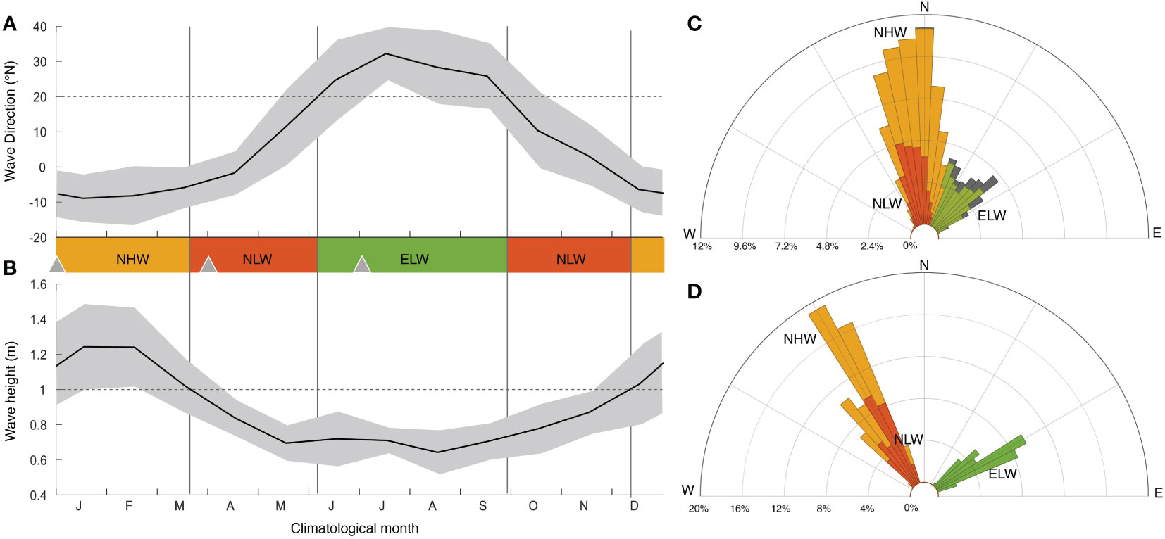
Figure 3 Characteristics of the surface wave forcing: Observed seasonal climatology of the significant wave height (A) and the wave direction (B) at the LTER1 fore reef site, constructed from the monthly averages of the data obtained in 20 minutes intervals from 2004 through 2018 (Washburn, 2019). (C) Windrose histogram of the wind direction from daily averages of the same measurements between 2004 and 2018. The observations were grouped into three wind forcing regimes, i.e., a northerly high wave regime (NHW, yellow) with monthly wave heights > 1 m and waves coming from northerly directions (-20 to 20 °), a northerly low wave regime (NLW, red), which corresponds to waves from the same direction, but with monthly wave heights < 1 m, and a northeasterly low wave regime (ELW, green) with waves coming from northeasterly direction (20 to 60 °). (D) Windrose histogram of the hourly forcing used to run the model for the three wave forcing regimes. Shown in (B) as triangles are the starting days for the time-slice simulations for each of the three wind regimes. See text for details.

The boundary conditions of the wave model for these three wave regimes were constructed based on the hourly wave measurements from the model boundaries for the period from January 1st until January 17, 2007.

These measurements are directly used for forcing the NHW regime. As these were the only wave measurement at the domain boundaries available to us, we modified these measurements in order to obtain the forcing for the NLW and ELW regimes. For the NLW regime, we reduced the wave height by a constant factor of 3, without changing the temporal pattern of the measurements. For the ELW regime, we adjusted the NLW forcing further by turning the angle of the wave direction by 90°. The windrose histogram of these produced three circulation regimes span the range of the observed wave conditions very well (Figures 3C, D).

The atmospheric forcing of each wave regime was created from three-hourly atmospheric measurements of solar radiation, wind velocity, air temperature, air pressure, humidity and rain obtained at the Gump research station located on the north-shore of Moorea Moorea (Washburn, 2020). Atmospheric pCO₂ is held fixed at 380.2 μatm, the mean value for Moorea between 2004-2018, computed from the marine boundary layer background dry air CO₂ mixing ratio product of NOAA (https://gml.noaa.gov/ccgg/mbl/mbl.html#ghg_product) as provided by Landschützer et al., 2020.

3.2.3 Lateral ocean boundary forcing

Because of the insufficient in-situ observations, we used global data products to construct the oceanic conditions at the northern lateral boundary for all wave regimes. The boundary conditions for temperature, salinity, and oxygen were specified on the basis of the monthly data from the World Ocean Atlas 2013 (Garcia et al., 2013; Locarnini et al., 2013; Zweng et al., 2013). Velocity fields were taken from Simple Ocean Data Assimilation (SODA) Version 2.0.2 (Carton and Giese, 2008). Surface DIC and TA at the lateral boundary were computed from the monthly OceanSODA-ETHZ dataset (Gregor and Gruber, 2021) using the years 2004-2018. These surface concentrations were extended to depth with respect to the mean vertical profiles of DIC and TA from the gridded product of the Global Ocean Data Analysis Project Vs 2 (Lauvset et al., 2016). This permitted us to retain consistency between the specified atmospheric CO₂ concentration and the surface and subsurface DIC fields.

3.2.4 Bottom coverage

For the bottom coverage, we used the average observed coverage of each benthic group between 2006 and 2018, thus neglecting the large temporal variations observed over the last few decades. The average bottom coverage for the corals during this period amounted to 25% in the fore and back reefs, and 20% in the fringing reefs (Edmunds, 2020). The coverage of macroalgae varied usually in an anti-correlated manner to that by the corals, with a mean of 10% in the fore and back reefs, and 5% in the fringing reef. Turf algae have the highest coverage, amounting to 30% in the fore and back reefs, and 15% in the fringing reef. Crustose coralline algae, sand and rubble are responsible for the remaining fractional coverage.

While our standard configuration neglects the potential contribution of turf- and macroalgae to coral reef metabolism, we constructed a sensitivity case wherein we parameterized this contribution (details provided in Supplementary Material).

3.2.5. Simulations

All simulations started from rest and were run for a total of 16 days (i.e., the number of full days the model can simulate in 24 hours on the supercomputer). The time-slices started on the virtual dates January 1, April 1 and July 1 to represent the NHW, NLW and ELW regimes, respectively. Initial conditions for all considered state variables, i.e., temperature, salinity, DIC, TA, and O₂ were based on measurements collected at the LTER1 and LTER2 sites (Figure 1). At these sites, monthly measurements were undertaking across the entire water column in the fringing, back and fore reefs as well as the top 75 meters of the open ocean. These observations were binned, and then vertically and horizontally interpolated to the entire model domain.

Previous studies had estimated that the water spends approximately 3 hours over the reef, but can remain in the system an average of 2 days if it enters the bays (Herdman et al., 2015). Based on this, we consider the first two days as spin-up, and used the remaining 14 days for the analyses. Annual mean properties of all fields are estimated by combining the model results for three wave regimes in a weighted manner such that the weight of each wave regime corresponds to normalized relative occurrence of that wave regime throughout the year (see Figure 3). Concretely, the results from the NHW regime were weighted 46%, those from the NLW 29% and those from the ELW 25%, where the total adds up to 100%.

3.3 Analyses tools

3.3.1 Carbonate chemistry

The derived properties pH, pCO₂, and Ω_α are computed from the model simulated DIC and TA employing the carbonate chemistry module mocsy 2.0 (Orr and Epitalon, 2015) and using the model simulated temperature, salinity, and nutrientconcentration as input. For these calculations, we use the dissociation constants for the carbonate system of Millero (2010). pH is thereby computed on the seawater scale.

3.3.2 Clustering

In order to reduce the time-space complexity of the results, we cluster the model domain into a set of regions that share common diel variability pattern in carbonate chemistry. To this end, we employ a K-Means clustering algorithm (Likas et al., 2003) with the annual mean diel cycle of pH over the entire model domain as input. We chose this property as its diel variability is representative for those of the other properties of the seawater carbonate system, especially that of Ω_α (see later). We identified three distinct clusters from the resulting dendrogram, taking into consideration also the requirement of a maximal silhouette value, (Lletı et al., 2004). This choice was further checked by performing Kruskal-Wallis tests (Kruskal and Wallis, 1952) to identify the statistical differences between the three clusters under the NHW, NLW and ELW wave regimes for pH, DIC, TA, and Ω_α. The test results confirmed that the clusters are statistically well separable (i.e., have p-values less than 0.01) for all parameters and wave conditions. The results of the Kruskal-Wallis tests, as well as the dendrogram and the computed silhouette values are provided in the supplementary materials.

3.3.3 Lagrangian analyses

In order to investigate the flow pathways in the reef system and to compute how much time the water spends over specific parts of the reef (i.e., to estimate the residence times), we conducted a Lagrangian analysis using Ariane Version 2.2.8 (http://www.univ-brest.fr/lpo/ariane). To this end, we used hourly output (horizontal and vertical velocities) from each of the three time-slice simulations for the three wave regimes as input for Ariane. We seeded particles at day three of the simulation at the surface in each grid point located over the reef as well as in those ocean grid points within one kilometer of the reef. This seeding approach resulted in the release of a total of 9512 particles. After release, the particles are passively advected by the circulation. We tracked the particles until they leave the domain and computed how much time they spend over particular parts of the domain. This analysis is performed for each wave scenario separately, which permit us to see the changes in the residence times as a response to the wave set-up.

4 Results

4.1 Circulation

The model simulates distinct circulation patterns for each wave regime over the reef systems and in the ocean just north of them (Figures 4A–C). The intensity of the flow over the reefs varies primarily with the height of the waves, whereas the flow path is primarily related to the wave direction. During northerly wave regimes (NHW and NLW in Figures 4A, B), the flow over the central Viapahu reef splits into two branches, one feeding Paopao Bay in the east, and the other feeding Opunohu Bay in the west (see Figure 1 for names). A similar splitting occurs in the eastern reef. In contrast, when the waves come from the northeast in the ELW regime (Figure 4C), the circulation over the reefs rotates westward, strengthening the flows over the eastern reef, but generally weakening the flow over the central Viapahu reef. In particular, the circulation over the western end of the Viapahu reef becomes very sluggish (i.e. ~0.3 m s⁻¹ in NHW, ~0.1 m s⁻¹ in NLW and less than 0.05 m s⁻¹ in ELW).

FIGURE 4

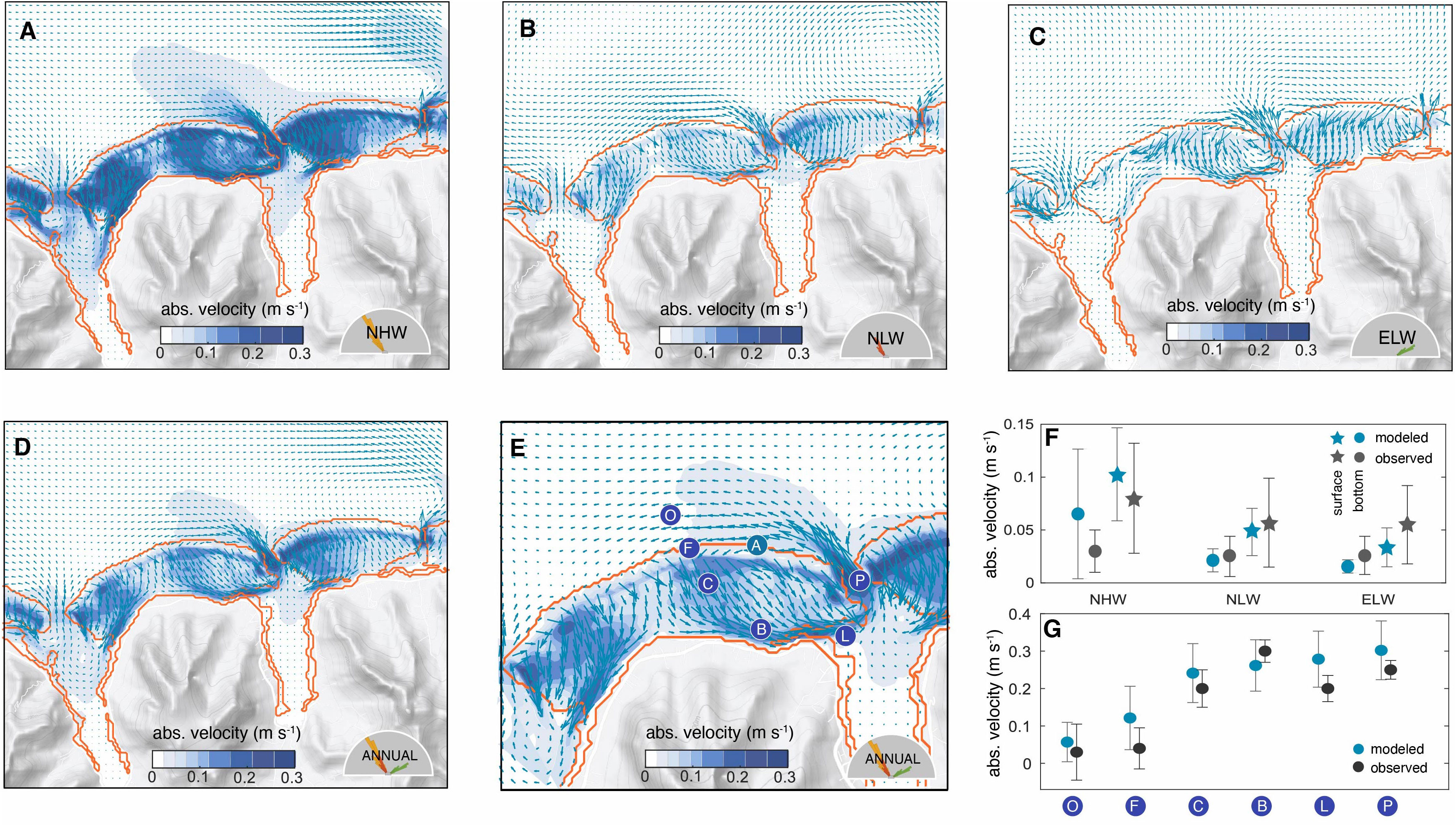
Figure 4 Model simulated circulation over the north-shore reefs of Moorea and evaluation with observations: Mean absolute velocity (shading) and direction (arrows) of the surface flows for the 14 days associated with the northerly high wave (NHW) regime (A), the northerly low wave regime (NLW) (B), and the northeasterly low wave regime (ELW) (C). Annual mean circulation constructed by combining the three wave regimes according to their relative frequency of occurrence (D) (see text for details), with a zoom and with the locations of the survey measurements of Hench et al. (2008) (blue circles) along a reef transect following the flow from the open ocean (O) to the lagoon (L) and to the pass (P) (E). Also shown as a circle (A) is the location of the long-term ADCP measurements at the LTER 1 site (Washburn, 2019) on the fore reef. (F) Comparison of the model simulated velocities with the long-term ADCP measurements at the LTER 1 site. The observation were stratified according to the wave regime and compared to the corresponding time-slice simulation. Shown are the mean results for the surface flows (triangles) and those at depth (circles), with the bars indicating the variability (one standard deviation). (G) Comparison of the model Hench et al. (2008) along the reef transect shown in (E). The circles indicate the mean over simulation period and the bars indicate the variability (one standard deviation). Since these measurements were taken during a NHW regime, we use the simulation results from this regime only for the comparison.

Under all scenarios, the majority of the water entering the reefs exits them within hours through the channels and then back out into the ocean through the passes in the forms of jets. The magnitude of these jets is mainly determined by the wave heights and less by the direction. Outside the passes, the waters are steered toward the west, largely in response to the anticlockwise circulation that circles the entire island and is present in all wave regimes. This strong westward steering prevents the waters from leaving the nearshore waters, causing also some recirculation back over the reef as these waters are transported onshore again by the wave action.

A small fraction of the reef waters enter the bays and contribute to the ventilation, especially at nighttime, when the waters lose buoyancy when being transported over the reef. This ventilation also replenishes the oxygen concentration of the bays (not shown). The circulation in the bays is more intense during the high wave regime, and differs little between the two low wave regimes.

The annual mean circulation, estimated from the weighted mean of the three wave regimes (Figure 4D), resembles the flow pattern of the northerly wave regimes. This primarily reflects the fact that these regimes dominate over the year, contributing together to 70% of all conditions. Within the Viapahu reef the annual mean flow speed highly varies from place to place, with certain parts of the reef experiencing typical flow velocities in excess of 0.2 m s⁻¹, while other areas are very sluggish, having typical velocities of less than 0.05 m s⁻¹. Thus, the circulation over the reef is highly structured with channels enabling rapid draining of waters and other areas where the waters remain relatively stagnant.

The model simulated circulation is very consistent with prior studies that described the flow characteristics based on observations and reef geometry (Hench et al., 2008; Leichter et al., 2012; Monismith et al., 2013; Herdman et al., 2015; Knee et al., 2016; Herdman et al., 2017). In particular, the modeled flow along the channels into the bays, and back out through the passes corresponds with the expectations. Quantitatively, the model simulated circulation compares excellently with the available observations, both with respect to magnitude and sensitivity to different wave regimes (Figures 4E, F).

The long-term current measurements from the fore reef, taken between 2004 and 2018 (Washburn, 2019), (circle A in Figure 4E) suggest an absolute surface ocean velocity of 0.08(±0.05) m s⁻¹ under NHW conditions, decreasing only slightly to 0.05 (±0.04) m s⁻¹ under either NLW and ELW conditions. The model simulates both the absolute values and the trend well, although perhaps with an overestimated sensitivity to the wave regime (Figure 4F). The model suggests a ~60% decrease in the surface absolute velocity under low wave conditions compared to those under high waves, which is higher than the reduction seen in the observations (~30%). The model also simulates the vertical shearing of the flow at the location of the measurements, with bottom currents being substantially reduced relatively to those at the surface (Figure 4F). However, the model tends to underestimate this vertical reduction up to 20%, particularly during high wave conditions.

The most important explanation for the discrepancy between the modelled and the measured flow velocities across the wave regimes is that the model is forced with idealized conditions constructed from observations stemming from January 2007, while the observations represent the long-term mean conditions for 15 years (2004-2018). Although we consider these constructed forcings as representative, they do not capture all conditions (Figure 3). For the underestimating of the vertical shear, we suspect that with our model’s resolution being 40x40 meters, it may not sufficiently resolve the geometry of the region and smaller scale variations in the bottom drag generated by the coral canopy structure. As a result, this may prevent our model from fully capturing the strong reduction in flow speed with depth in the NHW regime.

Spatially, the model captures well the observed acceleration of the flow along the typical path from the open ocean over the fore and back reefs, into the lagoons, channels, and then out through the passes Figure 4G). The model simulated velocities are, on average, slightly higher than the observed ones (by about 0.03 m s^-1), but this difference is well within the uncertainties arising from the temporal variability of the circulation. Further, these observations stem from December 2004 through January 2005 (Hench et al., 2008), where the wave conditions corresponded to the NHW regime, but still differed from those in 2007 used here. In summary, COAWST performs in our northern shore of Moorea setup excellently against the observational metrics, both with respect to flow pattern and velocities.

4.2 Coral metabolism

The coral polyp physiology model simulates a very active coral metabolism, characterized by strong diel fluctuations (Figure 5). Gross primary production (GPP) varies from zero at night to values up to 4 μmol m⁻² s⁻¹) (Figure 5A) driven by the day-night cycles of PAR. The variations in GPP between the different wave regimes are modest, but still notable with the NHW regime having the highest GPP, primarily owing to a faster rise in the morning hours. The model simulated GPP rates at mid-day are in very good agreement with those determined between 2006 and 2015 in the flume experiments (Carpenter, 2015) (Figure 5A).

FIGURE 5

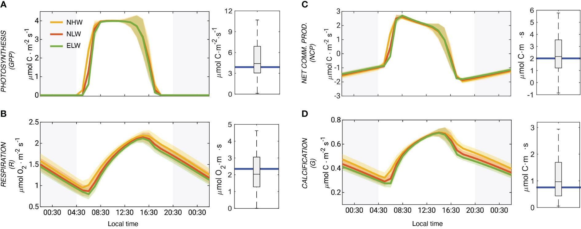
Figure 5 Model simulated coral metabolism and evaluation with observations: Mean diel cycle of net photosynthesis (GPP) (A), respiration (R) (B), net community production (NCP) (C) and coral calcification (G) (D) averaged over the entire domain. The comparison of model simulated mid-day rates with observations are given on the right side of each panel. The rates for the different wave regimes are indicated with different colors (NHW: yellow; NLW: red; ELW: green). The shadings indicate the variability (i.e., one standard deviation). The blue line shows the annual mean rates, computed from the weighted averages simulated for the three wave regimes. All rates are given as planar flux densities. The data are from Carpenter (2015) and other sources (see Supplementary Materials).

The simulated mid-day respiration (R) rates are about 2 μ mol m⁻² s⁻¹, again very comparable to the experimentally determined numbers (Figure 5B). Modeled respiration follows a distinct diel cycle with a minimum at sunrise and a maximum at around 16:00 local time. During the day, the modeled respiration rates are very similar across all wave regimes, but starting in the late afternoon and throughout the night, the NHW regime leads to distinctly higher respiration rates. This is a consequence of the higher diffusivity in this regime permitting a higher supply of oxygen from the surrounding seawater.

Over the course of the day, NCP varies from around -1 μmol m⁻² s⁻¹ at night to more than 2 μmol m⁻² s⁻¹ in the morning (Figure 5C). NCP declines during the day and relatively abruptly falls to below zero in the late afternoon. As was the case for GPP and respiration, the modeled rates for the mid-day fit the observations very well. Integrated over the day, NCP is slightly positive with a mean areal value of 0.005 μmol m⁻² s⁻¹.

The mid-day coral calcification rates are around ~0.6 μmol m⁻² s⁻¹ (Figure 5D). Even though they are a bit lower than the observed rates of 1±0.6 μmol m⁻² s⁻¹ determined from the flume experiments, they compare well within the large range of variability. The diel cycle of calcification follows that of respiration closely, which is a consequence of the high energy requirement for the pumping of protons out of the calcifying fluid into the coelenteron (Figure 2). The diel cycle of calcification is rather similar during the day across the three different wave regimes, but differs quite substantially during the night. The daily integrated rate of calcification is higher during the NHW conditions (41 mmol m^{−2 −1}) compared to the NLW and ELW conditions (36 mmol m⁻² s⁻¹ and 32 mmol m⁻² s⁻¹).

4.3 Carbonate chemistry

The model simulated interaction between the coral reef metabolism and the circulation over the reef systems of north-shore Moorea leads to distinct patterns in the annual mean conditions for the excess oxygen (oxygen levels above the saturation level) and the various parameters of the surface ocean carbonate chemistry (DIC, TA, pCO₂, pH, and Ω_α) (Figure 6). The waters are supersaturated with respect to oxygen nearly everywhere (5-20 mmol m^-3) (Figure 6A). For DIC and TA, the coral metabolism leads to a substantial depletion of the waters over the reef and the bays relative to the open ocean amounting to a mean difference of about 20 mmol m^-3 of DIC and 33 mmol m^-3 of TA for the quasi annual mean (Figures 6B, C). However, a closer inspection reveals some distinct differences. While DIC is most depleted relative to the open ocean in the bays, the maximum depletion for TA occurs over the back and fringing reefs of the main reef systems. These differences in the relative depletion pattern have substantial consequences for the other parameters of the seawater carbonate system, since all of them are very sensitive to changes in the ratio of TA over DIC (Sarmiento and Gruber, 2006). Concretely, the stronger depletion of TA over DIC over the back and fringing reefs of the Viapahu reef causes strong annual mean supersaturation in pCO₂ (around 300-400 μatm), and strong minima in pH (~-0.1) and in the saturation state Ω_α (~-0.5) in these sections of the reef system (Figures 6G–I). In contrast, the relatively similar depletion of TA and DIC in the bays causes none of these three properties to differ much between the open ocean and these regions, i.e., the effect of the reductions in TA and DIC on pCO₂, pH and Ω_α tend to cancel each other nearly completely.

FIGURE 6

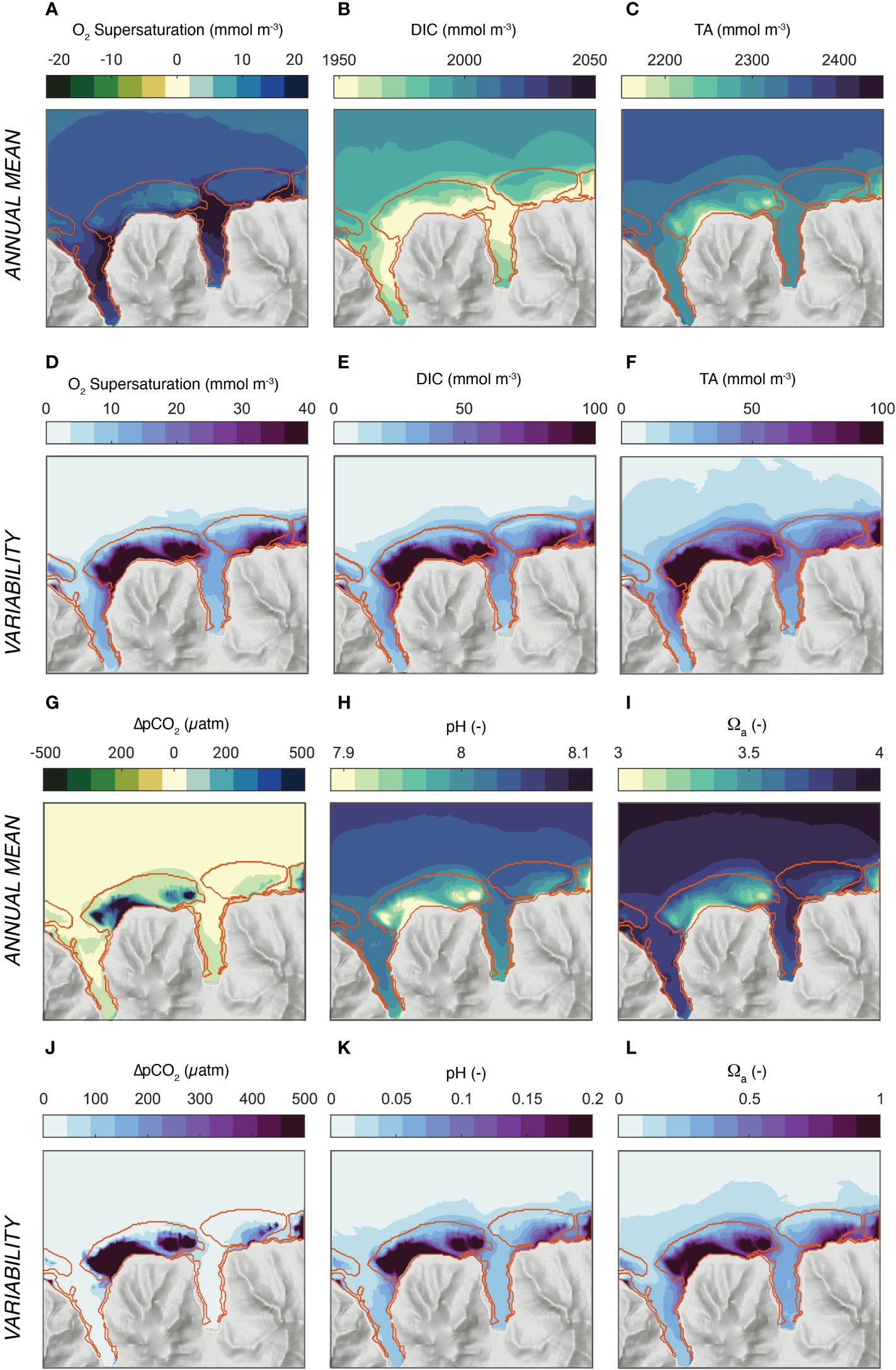
Figure 6 Simulated distribution of oxygen and the parameters of ocean carbonate system. (A-C) and (G–I) depict the annual mean concentrations, while (D-F) and (J-L) show the variability (one standard deviation). (A, D) Surface excess oxygen, i.e., O₂ - O₂ ^sat, (B, E) DIC, (C, F) Total Alkalinity (TA),(G, J) surface Δ;pCO₂ = pCO₂ - pCO₂ atm, (H, K) pH, and (I, L) Ω_a, the saturation state with respect to aragonite. The annual mean and standard deviations were computed from the simulations for the three wave regimes, taking into account their relative contribution to the annual cycle.

The annual mean gradients between the open ocean and the different sections of the reef are comparable in magnitude to the changes in the open ocean’s properties that have occurred since preindustrial times and are roughly similar to those expected for the next decades, even for a low emission scenario that is compatible with the Paris 2°C target (Bopp et al., 2013; Jiang et al., 2019; Kwiatkowski et al., 2020).

The modeled seawater chemistry compares reasonably well with the few available observations (Figure S2 in supplementary material). The model simulates the observed mean values within the observational constraints quite well, especially in the open ocean and in the fore reef sections. At the same time, the observations suggest a somewhat smaller gradient between the open ocean and the different sections of the reef. But the uncertainties in these comparisons are rather large, however. This is a consequence of the substantial representation errors associated with the very limited observations. None of these observations were taken as a synoptic survey, and thus pooling in time and space will likely result in an underestimation of the true gradients. This is especially the case when considering the very large temporal variations of the water column chemistry.

Figures 6D–F, J–L shows that the one standard deviation of the temporal variability is about two to three times larger than the mean gradient between the open ocean and the reef. The biggest variations occur over the back and fringing reef sections of the Viapahu reef with little difference between the different chemical properties. In general, the highest standard deviations occur in the regions where the largest difference to the open ocean occur, but the variability pattern between the different chemical properties is more similar to each other than the annual mean pattern. In absolute terms, the standard deviations amount to more than 100 mmol kg⁻¹ in DIC and TA, more than 300 μatm in ΔpCO₂, more than 0.2 in pH, and one unit in Ω_α. This corresponds to the level of variations found across the global surface ocean ocean (Sarmiento and Gruber, 2006; Gregor and Gruber, 2021). These high variations are limited to the main reef system. In contrast, the concentrations vary much less in the bays and over its fringing reefs. Also, the variability in the waters outside the fore reefs and in the passes are also comparably small.

The largest contributor to the simulated variability over the reefs is the diel cycle and is responsible for 99% of the simulated variability (Figure 7). At the same time, each chemical property has a distinct day-night pattern, especially over the reef systems. Oxygen is highly supersaturated during the day, but strongly undersaturated during the night hours (Figures 7A, D). DIC has the opposite pattern with a strong depletion during the day and a substantially elevated concentration relative to the open ocean during the night (Figures 7B, E). This is not the case for TA, whose mean daytime and nighttime concentrations barely change, maintaining the strong depletion relative to the open ocean conditions throughout the day (Figures 7C, F). This strong difference in the diel cycle between DIC and TA cause complex variations in pCO₂ (actually shown is $\Delta pC{O}_2=pC{O}_2-pC{O}_2^{\text{atm}}$, pH, and Ω_α (Figures 7G-L)). During the day, ΔpCO₂ is low relative to the open ocean over most of the back and fringing reefs. During the night, nearly the entire reef is highly supersaturated with respect to CO₂, causing high ΔpCO₂ relative to the open ocean. pH follows the same day-night asymmetry of pCO₂, just with the opposite sign. The same is the case for the saturation state Ω_α, although with a slightly shifted pattern.

FIGURE 7

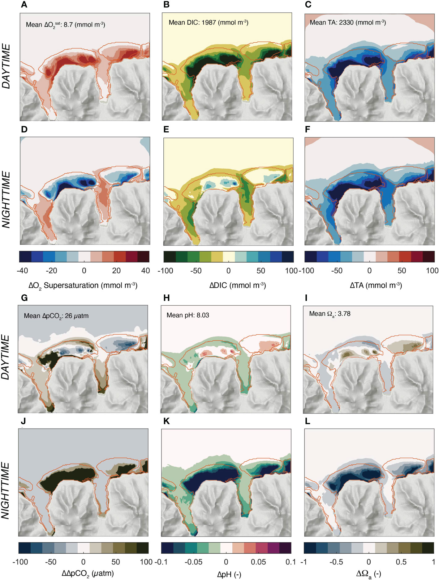
Figure 7 Simulated day and night distribution of oxygen and the parameters of ocean carbonate system relative to the open ocean. (A-C) and (G-I) depict the annual mean concentrations for the day hours, while (D-F) and (J-L) the same properties for the night hours. (A, F) Surface O₂ supersaturation, i.e., [O₂] - [O₂] ^sat, (B, E) DIC, (C, F) Total Alkalinity (TA),(G, J) surface Δ;pCO₂ = pCO₂ - pCO₂ atm, (H, K) pH, and (I, L) Ω_a, the saturation state with respect to aragonite. Also shown in (A–C) and (G-I) are the mean values for the open ocean. The daytime hours comprise 08:30 to 15:30, and the nighttime hours comprise the average of 21:30 and 04:30.

Thus, the interplay between the variability in ocean circulation and the strong diel changes in coral metabolism lead to a complex pattern of day-night changes in carbonate chemistry and oxygen that defy the expectations based on a purely local balance. Several specific questions emerge from these average pattern. First, what causes the day night asymmetry in DIC and TA over the reefs that then leads to the strong day-night asymmetries in ΔpCO₂, pH, and Ω_α? Second, what determines the pattern of the different chemical properties?

After the diel cycle, the second most important contribution to the temporal variability are the changes in ocean circulation and mixing imparted by the different wave regimes (Figure 8). To first order, the more sluggish circulation associated with the low wave regimes strongly enhances the pattern simulated by the high wave regime. This is particularly evident in the back and fringing reef sections of the Viapahu and eastern reefs, where, especially at night, the decrease in pH relative to the open ocean is highly accentuated. To second order, the shifts in the wave direction alters the pattern over the reef, especially in the western section of the Viapahu reef, where also the circulation changes most strongly with the change in wave direction (see Figure 4). Concretely, the usually elevated pH waters during daytime over the eastern section of the back and fringing reefs of Viapahu are replaced by rather low pH waters, such that this section of the reef remains lower than the open ocean throughout the day (Figure 8C). Similarly, although substantially smaller changes occur in the fore reef section of eastern Viapahu, the pH of the waters also remain lower than the open ocean all day. The latter feature can also be seen during the NLW regime (Figure 8B). This enhancement and pattern shifts in the pH resulting from the changes in the wave regimes (Figure 8) are also evident for all other investigated parameters (not shown).

FIGURE 8

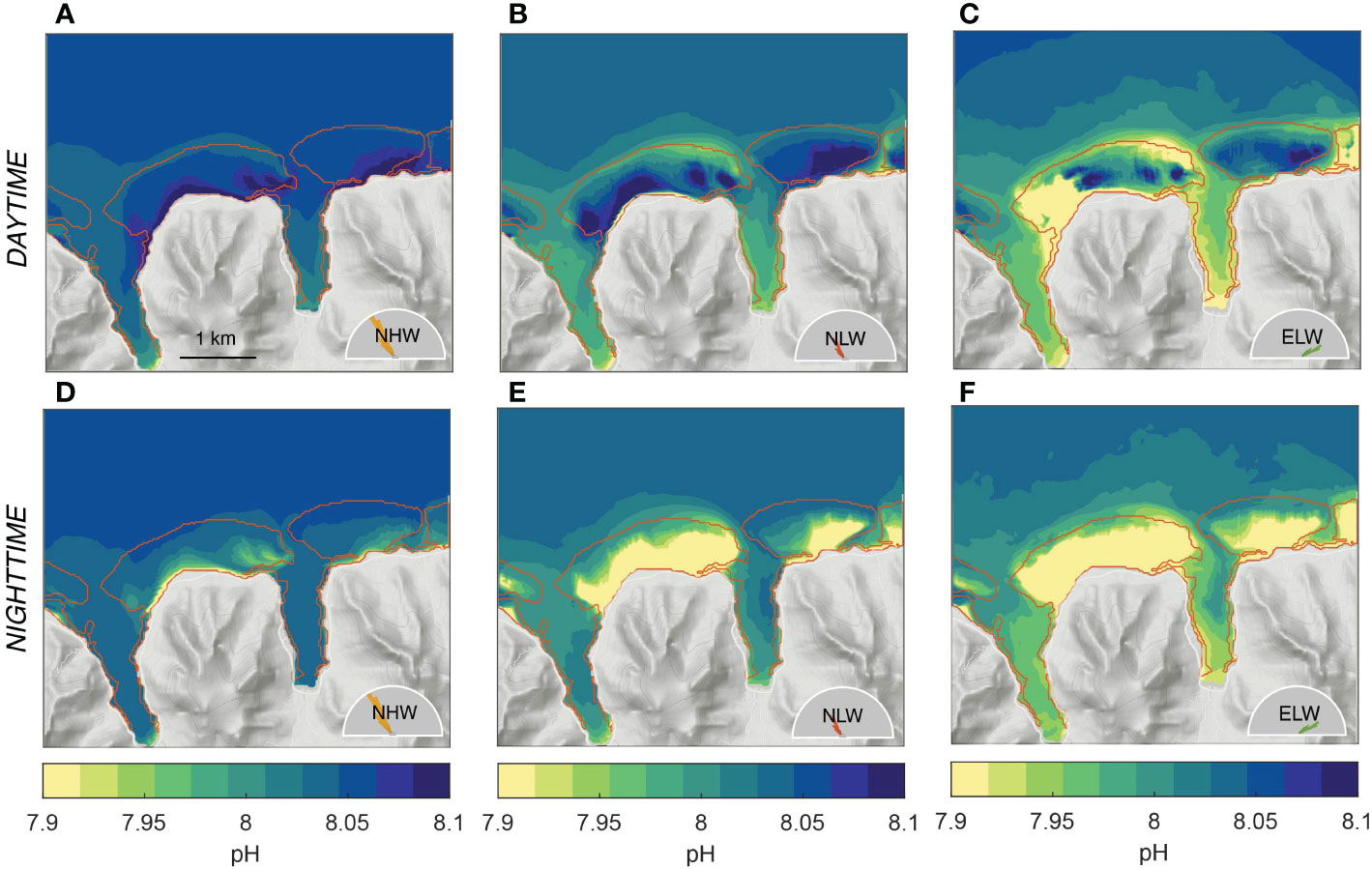
Figure 8 Simulated distribution of (top row) day- and (bottom row) nighttime pH for the three considered wave regimes, i.e., (A, D) northerly high wave (NHW) regime, (B, E) northerly low wave regime (NLW) and (C, F) northeasterly low wave regime (ELW). The weighted averages of these three scenarios for day and nighttime, respectively correspond to the annual mean shown in Figure 7H, K.

4.4 The emergence of biogeochemical niches

The K-means cluster analysis of the diel cycle of pH suggests that within the high spatiotemporal variability in reef’s carbonate chemistry, three clusters emerge (Figure 9A). These are: (i) an open ocean cluster that is characterized by chemical concentrations that are similar to the open ocean conditions, and with low diel variability (open ocean cluster, dark blue); (ii) a local cluster (light green) that is characterized with concentrations that deviate strongly from the open ocean conditions, and with high diel variability and, and (iii) an intermediate cluster (dark green) that is in between the two others. The clustering results were tested for their distinctness under the different wave regimes and for all other carbonate chemistry parameters and oxygen (see Method section 5.3 above for details). Also Figure (Figures 9B–G) confirms how different the chemical conditions are between the different clusters, both with respect to their mean and their variability and also vis-a-vis different wave regimes. Thus, these clusters can be viewed as distinct biogeochemical niches that are stable in place and time. Thus, the corals growing up in these different niches experience very different chemical conditions throughout their lifetime.

FIGURE 9

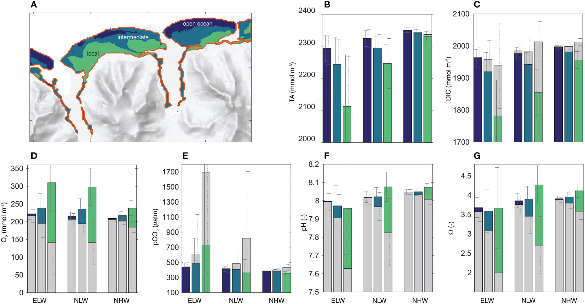
Figure 9 Emergence of biogeochemical niches: (A) Map showing the three biogeochemical niche clusters considered in our study. Average TA (B), DIC (C), dissolved oxygen (D), pCO₂ (E), pH (F) and the saturation state Ω_a (G) for each cluster (color) and each wave regime. Also shown is the diurnal range with the average day and average nighttime concentrations, with the colored column indicating the daytime concentrations, and the grey column indicating the nighttime concentrations. Since the two columns are plotted on top of each other with the taller bar in the back and the smaller one in the foreground, the diel range is given by the upper section of the column. If this section is colored (e.g., for O₂, pH, and Ω_a), then the daytime concentrations exceeds the nighttime ones. If the top section is grey (e.g., for DIC and pCO₂), then the nighttime concentrations exceed those during the day. The diel range of TA is too small to be clearly visible.

A more thorough inspection of Figure 9 reveals that with the exception of TA (Figure 9B), the lateral gradients in all parameters across the reef from the open ocean cluster (dark blue) to the local cluster (light green) vary fundamentally between day and night, highlighting the diel asymmetry noted above. In addition, the distinctiveness of the biogeochemical niches increases as the circulation over the reefs become more sluggish in the low wave regimes. The increase appears to be non-linear, with the amplitude of the diel cycle increasing more than the factor of three when comparing the ELW and NLW with the NHW regime. Especially the ELW regime leads to a high accumulation of the metabolic signature of the corals in the local niches, with pCO₂ levels at night reaching as high as 1700 μatm, pH levels as low as 7.6 and saturation states Ω_α as low as 2. The saturation state goes also below 3, on average, during the night hours of the NLW regime. This implies that corals in the local niches are every second night during the year exposed to chemical conditions that have been characterized as “extremely marginal” (e.g. Kleypas et al., 1999b).

4.5 Drivers determining the variability

A powerful way to analyze the effect of coral metabolism on the carbonate chemistry of the overlying water column is to plot the diel changes as a function of DIC (x-axis) and TA (y-axis) (Figure 10) (c.f. Smith, 1973; Suzuki and Kawahata, 2003; Cyronak et al., 2018). In such a plot, the impact of each of the three processes photosynthesis, respiration, and calcification can be represented by a distinct vector, reflecting their differential impact on the DIC and TA (Sarmiento and Gruber, 2006). The vectors describing the changes in DIC and TA during the photosynthesis and respiration are horizontal (we hereby neglect the impact on TA of the uptake of nitrogen by the corals and any subsequent reduction or oxidation process (Middelburg et al., 2020), a process that is considered negligible in coral reefs reefs (Chisholm and Gattuso, 1991), while calcification follows a vector with a slope of 2:1. In addition, this graph permits us to assess also the impact of these processes on pCO₂, pH, and Ω_α, since for constant temperature and salinity, these parameters have nearly linear isolines with a positive slope (thin lines in Figure 10).

FIGURE 10

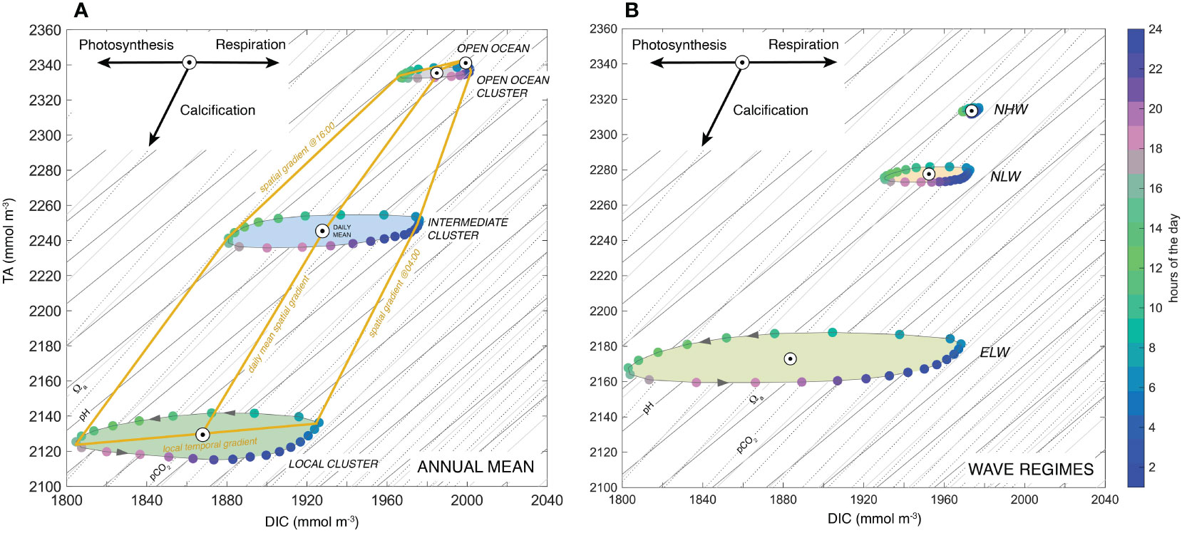
Figure 10 Processes determining the diel cycle of seawater chemistry: Variations of TA versus DIC across the reef system for the annual mean (A) and for the whole reef and for the different wave regimes (B). Shown are the diel progression in each of the three biogeochemical niche clusters. Colors indicate the hours of the day. Shown are also the isolines for pH (dark-grey line), pCO₂ (grey line) and Ω_a (dashed line). The arrows at the top left indicate how the processes of photosynthesis/respiration and calcification change seawater chemistry.

The die TA to DIC changes for the different clusters (Figure 10A) or for the different wave regimes (Figure 10B) describe ellipses, with main axes that have TA to DIC slopes of about 0.16, reflecting the dominance of coral NCP over coral calcification over the diel cycle (roughly by a factor of three to one). During the day, the high rates of NCP drive down DIC very rapidly until the afternoon hours, when NCP starts to decrease, eventually becoming negative at around 16:30 local time (see Figure 5G). At this time, calcification actually just passes its maximum (see Figure 5H), leading to a strong decrease in TA, while the calcification driven draw down in DIC is increasingly compensated by the production of DIC by respiration. This causes the diel cycle in the TA versus DIC diagram (Figure 10A) to turn around. It starts its back trajectory at around 18:00 local time, driven now by the fast increase in DIC caused by the strongly negative NCP owing to respiration no longer being balanced by photosynthesis. Since calcification continues throughout the night, this back-trajectory occurs at a lower concentration of TA, explaining the ellipsoid nature of this trajectory. As the calcification rates get weaker during the night, the impact of ocean circulation becomes more dominant, resupplying TA from the upstream clusters and ultimately from the open ocean. This resupply of TA (and DIC) permits the diel ellipse to close in the very early morning hours. The small tilt of the ellipse contrasts with the slope of the isolines for pH, pCO₂, and Ω_α, explaining why locally, the diel cycle causes large fluctuations in all these parameters.

The situation is very different when analyzing the average spatial gradients between the open ocean and the reef sections for different hours of the day (yellow lines in Figure 10A). During the late afternoon hours these gradients largely follow lines of near constant pH, pCO₂, and Ω_α. This contrasts strongly with the situation in the early morning hours, when the spatial gradients across the reef cross the isolines for pH, pCO₂, and Ω_α, leading to increases in these quantities, even though TA is decreasing. In the daily mean, the spatial gradients are in between these two extremes i.e., having a TA to DIC slope of 1.8, a value close to the calcification relationship of 2. This strongly reflects the fact that in our model, calcification is not balanced by any form of dissolution of CaCO₃, while GPP and R are nearly balanced, giving a near zero NCP over the course of a day.

The position of the ellipses within the TA versus DIC diagram for the different wave regimes (Figure 10B) indicate that the more sluggish the regime, the larger the ellipsoid, the larger its minor axis, and the stronger the deficit in TA relative to the open ocean (see also Figure 8). Similarly, the ellipses get larger and TA reductions get stronger from the open ocean to the local cluster (Figure 10A). The temporal slopes remain roughly the same within the clusters, i.e., about 0.16 (Figure 10A), although they are enhanced from high wave to low wave and northern to eastern wave conditions (Figure 10B).

4.6 Role of (re)circulation

In order to better understand the role of ocean circulation in driving the pattern over the reef and the formation of the biogeochemical provinces, we use the results from the Lagrangian experiments where we released particles in the water column (see section 3.3.3) and traced them through time. The trajectories of all tracked particles (Figures 11A–C) reveal a complex dynamics (see also Herdman et al. (2017)). Some particles circulate once over the reef and leave the reef system after their exit through the passes, while other particles recirculate many times over the reef before leaving (Figure 11D). Yet another group is primarily involved in circulation within the bays after having passed through the reef. The average single-pass transit time for the particles is short for most parts of the reef, ranging between 0.7 to 1.1 hours for the NHW regime (Figure 11E). In the low wave regimes, the transit time increases to 3 to 4 h, and in the case of the western most region of the Viapahu reef up to more than 7 h. The distribution of transit times is quite broad, with a standard deviation of the same order of magnitude as the mean transit time.

FIGURE 11

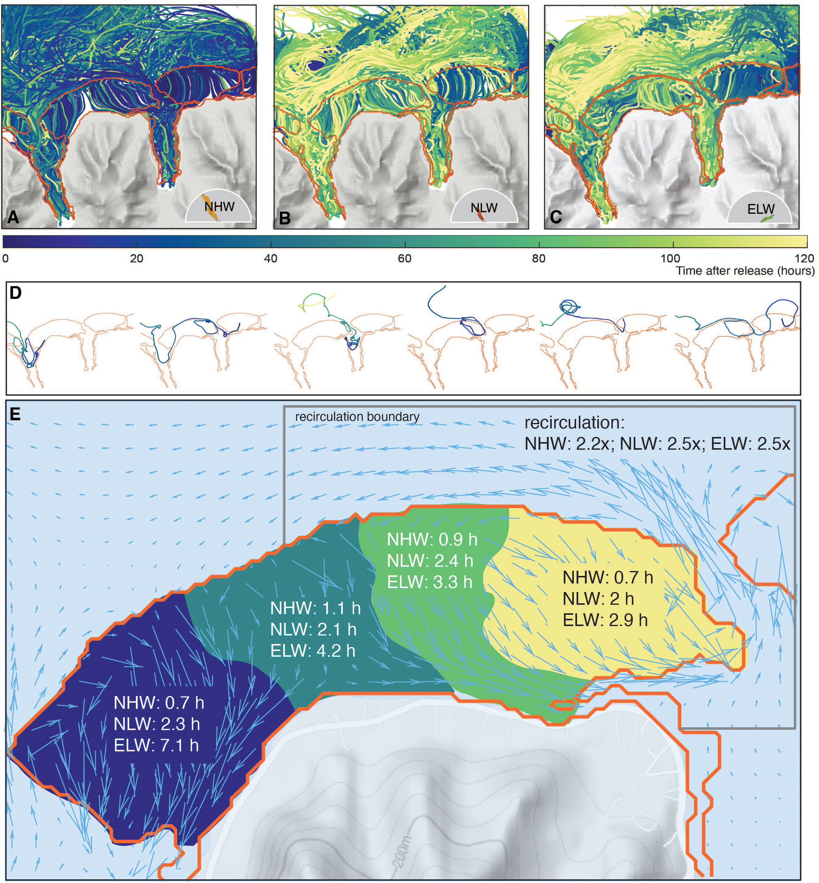
Figure 11 Circulation and flows over the reef system diagnosed from the Lagrangian simulations: Trajectories of all particles for the NHW wave regime (A), NLW wave regime (B) and ELW wave regime (C). Color indicates the time passed since the release. (D) Trajectories of selected particles. Colors are as in (A-C). (E) Diagnosed transit times over different sections of the Viapahu reef for the different wave regimes. Also shown are the number of times the average water parcel passes over the reef before it leaves the recirculation boundary delineated by the black line. The arrows in (E) depict the average flow in the NHW wave regime.

Combining these single-pass residence times with the typical metabolic rates and the water depth permits us to obtain a first order estimate of the expected variations in the different clusters. Using the typical daytime NCP rates of about 2 μmol m² s⁻¹ and the typical calcification rates G of about 0.6 μmol m2 s −¹, and taking into account the water depth (~2 m) fractional coverage of corals (25%) and the real-to-planar ratio (4), one would expect a DIC drawdown of ~3.6 mmol m⁻³ and a TA drawdown of ~1 mmol m⁻³ within 1 hour (in 12 hours the corresponding drawdowns are ~40 mmol m−³ for DIC and ~13 mmol m⁻³ for TA). These single-pass drawdowns are several times smaller than the modeled magnitude of the diel variability in Figure 10A. Thus, while differences in the single pass residence times are important for creating the distinct clusters, the effective residence time of typical waters over the reef must be much longer.

The Lagragian tracking permits us to count the number of times a water parcel passes over the reef before it leaves the system and to also compute the total amount of time it spends while doing so. Using 1 km from the fore reef as the distance of separation of oceanic regions and regions under the influence of corals (corresponding roughly to the outer position of the jet sitting in front of the fore reef (see grey line in Figure 11E), we find that the typical parcel traverses the reef about 2-3 times before it leaves the system, with the sluggish circulation regimes characterized by a slightly higher number of recirculations. The variance is large, with a few particles recirculating as much as 10 times before they leave the coral reef system. Consequently the actual time the water parcel spends over the reef is about 2 to 3 hours under high wave conditions on average, but this time increases to 10-12 hours under low wave conditions. Thus, recirculation of waters that leave the passes is a critical process for creating the strong spatio-temporal variations over the reefs.

5 Discussion

5.1 Spatio-temporal variability and the emergence of a mosaic

It is well understood by earlier studies that the interaction of reef metabolism and the circulation over the reefs leads to large biogeochemical variations, especially on diel scales (Suzuki and Kawahata, 1999; Bates, 2002; Suzuki and Kawahata, 2003; Manzello, 2010; Anthony et al., 2011; Kleypas et al., 2011; Gray et al., 2012; Falter et al., 2013; Teneva et al., 2013; Andersson et al., 2014; Albright et al., 2015; Kealoha et al., 2017; Takeshita et al., 2018; Yan et al., 2018). But our work provides new insights about the nature of this variability. First, the variability is not random in time and space, but it is spatiotemporally strongly structured, creating a mosaic of conditions that the organisms living in the different sections of the reef are exposed to. Second, the structure of the mosaic differs distinctly between the different biogeochemical parameters. Third, the diel variations describe a path dependency as shown by an ellipsoid when the trajectory is analyzed in phase space.

The structured spatial variability in biogeochemical conditions has not been discussed yet in the literature. One likely reason is that the observations tended to have been taken either at a fixed location, or as a (temporally limited) survey, preventing scientists to uncover the space-time mosaic. The second reason is that most model studies have used lower dimensional models (e.g., 1 D channel models, (Kleypas et al., 2011)) or idealized settings (e.g., Falter et al., 2013), where this biogeochemical patterning does not occur. Thus, for the detection of this time-space mosaic, it was crucial to simulate seawater carbonate chemistry in three-dimensions with realistic topography and for different wave and hence flow regimes.

Our model simulations permit us to identify the ingredients needed to create this time-space mosaic. The first ingredient is the structured nature of the circulation over the reef, i.e., the fact that the flow over the reef follows preferential paths, largely associated with topographic features, especially the presence of channels. Here the flow is fast, leading to short residence times. In contrast, the flow over other reef sections, especially sections of the back and fringing reefs, is very sluggish, leading to long residence times. In addition, much of the waters that have passed over the reef and then exit the bays through the passes reenter the reefs again, owing to a rather effective retention of the exiting waters. This recirculation is essential for creating the large gradients in biogeochemical conditions, sincethe waters accumulate the metabolic imprint during multiple passes the reef over the course of a single day. The pattern of this structured flow changes relatively modestly with wave regimes, being most sensitive to wave direction while the wave height changes only the flow speed, but not the path.

Being the primary driver of the circulation over reef system, the wave forcing determines the residence times (Hench et al., 2008; Monismith et al., 2013), and hence the amplitude of the biogeochemical variability. It is larger in the low wave scenarios compared to high wave scenarios. This amplification of biogeochemical variability with the elevated wave height is more than the one expected based on the scaling argument of Falter et al. (2013). Using idealized three-dimensional simulations, they suggested that the amplitude of the diel cycle scales inversely with the significant wave height forcing of the reef system, i.e., that the factor of three reduction in the wave forcing between the NHW and NLW regime should lead to a factor of three increase in the diel amplitude. Our simulations indicate an increase of more than a factor of four, and in the case of the ELW wave regime, up to a factor of 10 locally.

Such a structured flow has been seen in other three-dimensional simulations of the circulation over coral reef ecosystems (Falter et al., 2013; Watanabe et al., 2013; Nakamura et al., 2018) and to a limited degree with observations, especially with Lagrangian experiments. Also the strong retention of the waters exiting the passes, forcing a strong recirculation has been observed and modeled (Herdman et al., 2017). It is intriguing to note that this recirculation is not only essential for enhancing the spatio-temporal gradients over the reef by water parcels accumulating the metabolic signals over multiple passes over the reef, but also for critical ecological and biogeochemical functions such as the retention of larvae and nutrients (Leichter et al., 2013). In summary, we conclude that the highly structured flow over the reef is a robust finding, especially also since the evaluation of the model simulated flow with the observations gave excellent results. Thus, in order to understand how coral metabolism interacts and modifies the overlying seawater chemistry, we consider it critical to go beyond the one dimensional channel flow concept (see e.g. Kleypas et al., 2011), i.e., a unidirectional flow of water over the coral reef with the waters accumulating the metabolic imprint along this path.

The second ingredient generating this mosaic of conditions and especially the distinct spatio-temporal gradients in the considered biogeochemical parameters is the diel cycles of NCP and calcification. For example, during the day, compensatory effects between positive NCP and calcification lead to very small spatial gradients in pH, pCO₂, and Ω_α, while at night, negative NCP and calcification reinforce each other, creating very strong gradients in these properties. In contrast, DIC and O₂ vary quite symmetrically during day and night. Lastly, TA shows a sustained depletion throughout the day. While the detailed temporal evolution of NCP and calcification in our model simulations are associated with substantial uncertainties owing to these processes being modeled without strong observational constraints, the fundamental driving force, i.e., the day-night pattern of NCP is determined by the availability of light and thus robust.

5.2 Implications

The spatio-temporal patterning in reef’s carbonate chemistry has important implication for the determination of the reef metabolism from the spatio-temporal gradients of TA and DIC (e.g., Gattuso et al., 1993; Gattuso et al., 1996; Watanabe et al., 2006; Shamberger et al., 2011; Kwiatkowski et al., 2016). In our model, the slope of the TA to DIC relationship is only about 0.16 when analyzing the diel cycle locally, while this slope varies between ~1.4 and 3.4 when analyzed spatially (Figure 10). Our finding of strongly varying ratios as a function of scales in time and space supports the results of Takeshita et al. (2018) who surveyed the reef system in Bermuda, and also found a slope of about 0.2 when the data were analyzed temporally, and a slope of about 1 when they analyzed the large-scale gradients. Thus both our results and those of Takeshita et al. (2018) support the hypothesis of Cyronak et al. (2018) who suggested on the basis of their meta-analysis that the temporal and spatial approaches to estimate the reef metabolism yield fundamentally different perspectives. Our model simulations reveal that the situation is even more complex, as the slope is always a combination of the temporal (i.e., local) perspective reflecting primarily the diel cycle of NCP, and of the spatial perspective reflecting primarily calcification. If the interplay of these temporal and spatial perspectives are not taken into account, the estimates of the reef metabolism are accordingly biased and might require a reassessment of many published results.

The emergence of biogeochemical niches within the spatio-temporal patterning of the biogeochemical properties over the reef has important implications for assessing the reef’s potential resilience to future ocean acidification. It is well known that preconditioning of organisms to future change through high variability has strong implications for their potential vulnerability (e.g., Comeau, 2014; Oliver and Palumbi, 2011; Rivest et al., 2017). For example, based on the survey conducted by Rivest et al. (2017), corals calcify less under constant pH compared to a pH that has the same mean value, but fluctuates in time. Similarly, coral larvae exposed to high pH variations over 3-6 days exhibit up to 18% higher survival rate than larvae raised under constant ambient pH Dufault et al. (2012). Furthermore, diel oscillations in pCO₂ are shown to lessen the reductions in calcification due to ocean acidification Comeau (2014). Thus, corals from regions of high pH variability are expected to cope much better with future ocean acidification than those from a low variability region.

Based on the meta-anaylsis of studies that have investigated the effects of natural CO₂ variability on coral susceptibility to ocean acidification (Kapsenberg and Cyronak, 2019), this strong reduction in vulnerability in response to exposure to variability primarily happens through local adaptation. When the organisms are exposed to harmful conditions for more than one generation, their adaptive capacity is boosted through natural selection, e.g., by shifting community composition of corals and/or their symbionts toward an increased abundance of more tolerant genotypes. Hence, one would expect that different coral lineages growing in different biogeochemical niches might have developed different adaptations potentials, with corals of historically highly variable carbonate chemistry conditions being substantially more resilient to ocean acidification. This implies that on the north-shore of Moorea, one would expect individuals from the local cluster that is characterized by high concentrations and high variability to cope better with external stressors. This could provide also an opportunity for restoration projects.

In contrast, our work provides little support for the presence of ocean acidification refugia (Manzello et al., 2012; Kapsenberg and Cyronak, 2019). At the spatio-temporal scales investigated here, conditions within the reefs are almost always more acidic (lower pH) and have lower saturation states Ω_α relative to the open ocean. As discussed above, this is a consequence of the fact that during the daytime NCP and calcification nearly balance each other in terms of their impact on pH and Ω_α, while at night, the impact of NCP and calcification enhance each other.

The final implication concerns the determination of the CO₂ source/sink behaviour of a coral reef. The spatio-temporal patterning requires a structured sampling design in order to correctly determine the mean oceanic pCO₂ over the reef system. Even though the average modeled pCO₂ does not exceed the atmospheric pCO₂ by much, the northern shore reef systems of Moorea are modeled to be an overall source of CO₂ to the atmosphere, reflecting primarily the fact that over the diel cycle, NCP is close to zero while calcification constitutes a substantial net sink for TA. This yields a long-term NCP to calcification ratio of near zero, much lower than the critical value of 0.6 needed for a coral reef system to be a net CO₂ sink from the atmosphere (Suzuki and Kawahata, 2003).

5.3 Caveats and limitations

A set of caveats of this study stems from the simplifications done during model development. First, we only consider one type of coral in our model. Therefore, we underestimate the amount of variance across the reef. For example, recent flume experiments in Moorea suggested substantial community differences in the relative rates of NCP and calcification (Lantz et al., 2017). Furthermore, the model accounts for the coral coverage variability between the fore reef, back reef and fringing reef section, but does not resolve the variability within them. In fact, spatial variability in coral assemblages within reef types introduce variability in the imprint of the corals on the seawater. This effect would be less prominent in fast flowing reef sections as this imprint is quickly mixed along the flow pathway. However, it would be essential in regions with low flow rates and/or under low wave conditions. But already with the current one coral model, the model generates highly variable biogeochemical conditions giving rise to distinct biogeochemical niches.

Second, we also do not consider the contribution of other metabolically active benthic components on the reef, namely turfalgae, macroalgae, calcifying algae and sandy regions. When we included the contribution of turf- and macroalgae to reef metabolism, as done in our sensitivity simulation, the fundamental insights gained in this study are actually accentuated, i.e., the variability in biogeochemical conditions become more distinct. This is because the consideration of these additional autotrophic plants leads to even stronger day-night differences in NCP. If these non-calcifiying benthic algal groups were present in the model, one would expect to see an increase in pH and Ω_α toward the shore during the day. This would potentially lead to formation of a daytime refugium, which is not present in the current version of the model. However, such a daytime refugium would be lost during the night, when the pH would decrease even more owing to intensified respiration.

The neglect of calcifying algae (i.e., crustose coralline algae), whose metabolic effect on the overlying seawater chemistry is similar to that of the corals, also has a moderating effect on our results. Since they have been shown to contribute up to 25% to the total photosynthesis and calcification rates on the Moorea coral reefs (Comeau et al., 2016; Comeau et al., 2017), the level of our model simulated variability could be correspondingly underestimated. But the coverage of the bottom by calcifying algae varied greatly in the last decades (32±21% (Edmunds, 2020)), such that the degree of underestimation would strongly depend on the actual relative abundance of coral and calcifying algae in the region.

Lastly, our neglect of the potential dissolution of CaCO₃ in sandy regions leads to a tendency in our model to overestimate net calcification, i.e., reduce the net sink of the coral reef system for TA. However, we expect only a limited impact of this neglect on our core results. This is primarily because CaCO₃ dissolution in coral reefs is primarily observed at nighttime, and at rates ranging between 0.1 and 4 mmolC ^-2h^-1 (i.e., 0.09 and 3.50 kg m^-2yr^-1 (Andersson and Gledhill, 2013). Thus, a rough estimate of the carbonate dissolution for our system (i.e., ~25% coverage of the bottom by sands (Edmunds, 2020) and a water column depth of 2 meters) would result in an increase of 1.5-6 mmolC m^-3 in DIC and 3-12 mmol m^-3 in TA, respectively over the 12 hours of nighttime. This is much lower than the simulated diel variations in DIC and TA. Thus, incorporating the dissolution of carbonate sands in our model would have little impact on our findings with regard to the emergence of the biogeochemical niches. But it would lead to a reduced loss of TA and hence a smaller gradient from the open ocean toward the reef, a smaller overall outgassing of CO₂, and a smaller spatial slope in the TA versus DIC. The latter would bring this slope closer to that seen in other coral reefs.

Another caveat of this study is the lack of consideration of bubble-mediated transfer of gases across the air-sea interface. This process is known to contribute to the oxygen supersaturation in surface waters (Craig and Hayward, 1987), as breaking waves are known to push extra oxygen into the ocean (Keeling, 1993; Deike and Melville, 2018). Recently, Reichl and Deike (2020) suggested that the contribution of this effect for CO₂ may be as large as 40% of the air-sea exchange of CO₂. For oxygen, the relative contribution would be higher, as its solubility is more enhanced by pressure. However, the modeled impact of air-sea gas exchanges on the seawater CO₂ and O₂ variations are low (less than 1% of total diel variations, not shown) in agreement with previous work on reefs (Watanabe et al., 2006; Falter et al., 2013; Yeakel, 2015). Thus, we consider the bubble contribution to the exchange of CO₂ to be very small.

Data availability was an additional challenge in our study. As the data with which we evaluate our model are both scarce and sparse, the strength of the conclusions we draw from the comparison with the observations are limited. For instance, the model simulated strong biogeochemical gradients between the open water and the reef systems are not so evident in the observations (provided in Supplementary material). At face value, this comparison would suggest that either the modeled reef is metabolically too active or that the water circulation is too sluggish, leading to an overly strong accumulation of the metabolic imprint as the waters are flowing over the reefs. But, the abundant observations of the circulation do not suggest that the modeled circulation is too sluggish (Figure 4). Also the modeled metabolic rates are in the correct range, and if anything on the lower end of the observations Figure 5). Furthermore, several modeling studies demonstrated that coral metabolism tends to create strong lateral gradients in carbonate chemistry parameters over coral reefs and of similar magnitude as those modeled here (Kleypas et al., 2011; Falter et al., 2013). Thus, the discrepancy appears to be primarily caused by the available observations not being of sufficient density in time and space to compute a correct time-space mean over different sections of the reef. Similar challenges existed for evaluating the diel cycle of pCO₂ and the other variables of the seawater carbonate system. Yet again, the model simulated variations are entirely within the range of expectations given the measurements in other, comparable reef systems. Compared to the potential biases introduced by the model structure and its forcing, the uncertainties emanating from the potential errors in the dissociation constants of the marine carbonate system are negligible and are thus not quantitatively assessed.

While these caveats reveal the limits of our work, particularly with regard to the exact quantification of the space-time variations in seawater chemistry in the north-shore reef system of Moorea, they do not undermine the most important conclusions of our work, i.e., how the interplay between coral metabolism and reef circulation gives rise to a space-time mosaic of biogeochemical conditions.

6 Conclusion

The development and use of a dynamically coupled hydrodynamic/biogeochemical/physiological model to investigate the spatio-temporal variability of the biogeochemical conditions in the northern shore reef systems of Moorea led to important new insights that more traditional approaches would not have been able to achieve. Without the explicit modeling of the three-dimensional flow of waters over the reef into the lagoons and bays and then out through the passes and the detailed consideration of the temporal dynamics of NCP and calcification, the model would not have generated the strong spatio-temporal patterning that we highlighted in this study. Similarly, no distinct biogeochemical niches would have emerged in our results. We consider our results to be sufficiently generalizable to be applicable also for other coral reef ecosystems, i.e., we expect that nearly all reef ecosystems have a strongly patterned spatio-temporal dynamics in their biogeochemical conditions, including distinct biogeochemical niches. Thus our hypothesis that the existence of these niches could help and support genetic diversity within the reef by forcing local within niche adaptation could be investigated in all reefs. We also encourage studies to investigate variations in resilience to external stressors within reefs, as this could be exploited for assessing the health for reefs and potentials for recovery after a perturbation.

On the modeling side, several avenues can be pursued in the future. Not yet explored in our results are the impact of the spatio-temporal variability in the biogeochemical conditions on the rates of photosynthesis and calcification in our model, even though the model system is taking this two-way interaction already fully into consideration. This will be explored in a subsequent study. Further work requires a more extensive consideration of the diversity of the reef communities, especially the explicit consideration of turf-, macro- and calcifying algae, as well as fish and a representation of the biogeochemical fluxes in the sandy sections of the reefs. Such coupled models are ideally positioned to assess the impact of future climate change and ocean acidification on the local reef ecosystems, providing the tool of choice for the dynamic downscaling of large-scale results to the local system of interest. Our newly developed coupled system, although configured here for the north-shore of Moorea, is fundamentally flexible and can be configured for any other reef system, providing opportunities to generalize the conclusions beyond Moorea.

Data availability statement

The model output used for this study can be accessed freely at the ETH Research Collection under the link: https://www.research-collection.ethz.ch/handle/20.500.11850/559940.

Author contributions

This project was conceived by MM and NG. DD and MM set up the model. DD run the simulations and led the analyses. DD wrote the first draft of the paper with substantial input by NG, MM, and MV. NG led the revision of the paper leading to the final submitted version. NG and MM supervised this work.

Funding

This work received funding from the Tetiaroa Foundation. Additional funding was provided by ETH Zürich. Open access funding provided by ETH Zurich.

Acknowledgments

We thank Matthias Troyer for initiating the collaboration between ETH Zürich and the Gump Research Station at Moorea that led to this project and for his financial and intellectual support. We are grateful to James Hench and Walter Torres for providing us with the initial setup of COAWST including the topographic information and the forcing. We thank Damian Loher for his technical support. We are indebted to Sally Holbrook and Russ Schmitt who provided helpful advice and connected us to the people and datasets of the LTER. We thank the many investigators of the Moorea Coral Reef Ecosystem LTER, for providing their data sets and acknowledge its funding by the US National Science Foundation (OCE-1637396 and earlier awards).

Conflict of interest

The authors declare that the research was conducted in the absence of any commercial or financial relationships that could be construed as a potential conflict of interest.

Publisher’s note

All claims expressed in this article are solely those of the authors and do not necessarily represent those of their affiliated organizations, or those of the publisher, the editors and the reviewers. Any product that may be evaluated in this article, or claim that may be made by its manufacturer, is not guaranteed or endorsed by the publisher.

Supplementary material

The Supplementary Material for this article can be found online at: https://www.frontiersin.org/articles/10.3389/fmars.2022.1004107/full#supplementary-material

References

Albright R., Benthuysen J., Cantin N., Caldeira K., Anthony K. (2015). Coral reef metabolism and carbon chemistry dynamics of a coral reef flat. Geophys. Res. Lett. 42, 3980–3988. doi: 10.1002/2015GL063488

CrossRef Full Text | Google Scholar

Al-Horani F. A., Al-Moghrabi S. M., De Beer D. (2003). The mechanism of calcification and its relation to photosynthesis and respiration in the scleractinian coral galaxea fascicularis. Mar. Biol. 142, 419–426. doi: 10.1007/s00227-002-0981-8

CrossRef Full Text | Google Scholar

Andersson A. J., Gledhill D. (2013). Ocean acidification and coral reefs: Effects on breakdown, dissolution, and net ecosystem calcification. Annu. Rev. Mar. Sci. 5, 321–348. doi: 10.1146/annurev-marine-121211-172241

CrossRef Full Text | Google Scholar

Andersson A. J., Yeakel K. L., Bates N. R., De Putron S. J. (2014). Partial offsets in ocean acidification from changing coral reef biogeochemistry. Nat. Climate Change 4, 56–61. doi: 10.1038/nclimate2050

CrossRef Full Text | Google Scholar

Anthony K. R., Kleypas A., Gattuso J. P. (2011). Coral reefs modify their seawater carbon chemistry - implications for impacts of ocean acidification. Global Change Biol. 17, 3655–3666. doi: 10.1111/j.1365-2486.2011.02510.x

CrossRef Full Text | Google Scholar

Baird M. E., Mongin M., Rizwi F., Bay L. K., Cantin N. E., Soja-Woźniak M., et al. (2018). A mechanistic model of coral bleaching due to temperature-mediated light-driven reactive oxygen build-up in zooxanthellae. Ecol. Model. 386, 20–37. doi: 10.1016/j.ecolmodel.2018.07.013

CrossRef Full Text | Google Scholar

Bates N. R. (2002). Seasonal variability of the effect of coral reefs on seawater CO₂ and air-sea CO₂ exchange. Limnol. Oceanog. 47, 43–52. doi: 10.4319/lo.2002.47.1.0043

CrossRef Full Text | Google Scholar

Bindoff N. L., Cheung W. W., Kairo J. G., Arístegui J., Guinder V. A., Hallberg R., et al. (2021). Changing ocean, marine ecosystems, and dependent communities. IPCC special report on the ocean and cryosphere in a changing climate. 477–587.

Google Scholar

Bitter M. C., Kapsenberg L., Gattuso J.-P., Pfister C. A. (2019). Standing genetic variation fuels rapid adaptation to ocean acidification. Nat. Commun. 10, 5821. doi: 10.1038/s41467-019-13767-1

PubMed Abstract | CrossRef Full Text | Google Scholar

Booij N., Ris R. C., Holthuijsen L. H. (1999). A third-generation wave model for coastal regions 1. model description and validation. J. Geophys. Res.: Oceans 104, 7649–7666. doi: 10.1029/98JC02622

CrossRef Full Text | Google Scholar

Bopp L., Resplandy L., Orr J. C., Doney S. C., Dunne J. P., Gehlen M., et al. (2013). Multiple stressors of ocean ecosystems in the 21st century: projections with CMIP5 models. Biogeosciences 10, 6225–6245. doi: 10.5194/bg-10-6225-2013

CrossRef Full Text | Google Scholar

Boyd P. W., Cornwall C. E., Davison A., Doney S. C., Fourquez M., Hurd C. L., et al. (2016). Biological responses to environmental heterogeneity under future ocean conditions. Global Change Biol. 22, 2633–2650. doi: 10.1111/gcb.13287

CrossRef Full Text | Google Scholar

Carpenter R. (2015). MCR LTER: Coral reef: Estimates of component primary production and respiration. Available at: http://mcrlter.msi.ucsb.edu/cgi-bin/showDataset.cgi?docid=knb-lter-mcr.19.

Google Scholar

Carton J. A., Giese B. S. (2008). A reanalysis of ocean climate using simple ocean data assimilation (SODA). Monthly Weather Rev. 136, 2999–3017. doi: 10.1175/2007MWR1978.1

CrossRef Full Text | Google Scholar

Chisholm J. R., Gattuso J. (1991). Validation of the alkalinity anomaly technique for investigating calcification of photosynthesis in coral reef communities. Limnol. Oceanog. 36, 1232–1239. doi: 10.4319/lo.1991.36.6.1232

CrossRef Full Text | Google Scholar

Comeau S., Carpenter R., Edmunds P. (2017). Effects of pCO₂ on photosynthesis and respiration of tropical scleractinian corals and calcified algae. ICES J. Mar. Sci. 74, 1092–1102. doi: 10.1093/icesjms/fsv267

CrossRef Full Text | Google Scholar

Comeau S., Edmunds P., Spindel N. B., Carpenter R. C. (2014). Diel pCO₂ oscillations modulate the response of the coral acropora hyacinthus to ocean acidification. Mar. Ecol. Prog. Ser. 501, 99–111. doi: 10.3354/meps10690

CrossRef Full Text | Google Scholar

Comeau S., Carpenter R., Lantz C., Edmunds P. (2016). Parameterization of the response of calcification to temperature and pCO₂ in the coral acropora pulchra and the alga lithophyllum kotschyanum. Coral Reefs 35, 929–939. doi: 10.1007/s00338-016-1425-0

CrossRef Full Text | Google Scholar

Costanza R., “d’Arge” R., de Groot R., Farber S., Grasso M., Hannon B., et al. (1997). The value of the world’s ecosystem services and natural capital. Nature 387, 253–260. doi: 10.1038/387253a0

CrossRef Full Text | Google Scholar

Costanza R., de Groot R., Braat L., Kubiszewski I., Fioramonti L., Sutton P., et al. (2017). Twenty years of ecosystem services: How far have we come and how far do we still need to go? Ecosyst. Serv. 28, 1–16. doi: 10.1016/j.ecoser.2017.09.008

CrossRef Full Text | Google Scholar

Craig H., Hayward T. (1987). Oxygen supersaturation in the ocean. Biol. versus Phys. contribut. 235, 199–202.

Google Scholar

Cyronak T., Andersson A. J., Langdon C., Albright R., Bates N. R., Caldeira K., et al. (2018). Taking the metabolic pulse of the world’s coral reefs. PloS One 13, 1–17. doi: 10.1371/journal.pone.0190872

CrossRef Full Text | Google Scholar

Deike L., Melville W. K. (2018). Gas transfer by breaking waves. Geophys. Res. Lett. 45, 10,482–10,492. doi: 10.1029/2018GL078758

CrossRef Full Text | Google Scholar

Delesalle B., Pichon M., Frankignoulle M., Gattuso J. P. (1993). Effects of a cyclone on coral reef phytoplankton biomass, primary production and composition (Moorea island, French Polynesia). J. Plankton Res. 15, 1413–1423. doi: 10.1093/plankt/15.12.1413

CrossRef Full Text | Google Scholar

Dufault A. M., Cumbo V. R., Fan T. Y., Edmunds P. J. (2012). Effects of diurnally oscillating pCO₂ on the calcification and survival of coral recruits. Proc. R. Soc. B: Biol. Sci. 279, 2951–2958. doi: 10.1098/rspb.2011.2545

CrossRef Full Text | Google Scholar

Edmunds P. (2020). MCR LTER: Coral reef: Long-term population and community dynamics: Corals, ongoing since 2005. doi: 10.6073/pasta/10ee808a046cb63c0b8e3bc3c9799806

CrossRef Full Text | Google Scholar

Fabricius K. E., Langdon C., Uthicke S., Humphrey C., Noonan S., De’ath G., et al. (2011). Losers and winners in coral reefs acclimatized to elevated carbon dioxide concentrations. Nat. Climate Change 1, 165–169. doi: 10.1038/nclimate1122

CrossRef Full Text | Google Scholar

Falter J. L., Lowe R. J., Zhang Z., McCulloch M. (2013). Physical and biological controls on the carbonate chemistry of coral reef waters: Effects of metabolism, wave forcing, Sea level, and geomorphology. PloS One 8, e53303. doi: 10.1371/journal.pone.0053303

PubMed Abstract | CrossRef Full Text | Google Scholar

Feely R. A., Doney S. C., Cooley S. C. (2009). Ocean acidification: Present conditions and future changes in a high-CO₂ world. Oceanography 22, 36–47. doi: 10.5670/oceanog.2009.95

CrossRef Full Text | Google Scholar

Frankignoulle M., Gattuso J. P., Biondo R., Bourge I., Copin-Montégut G., Pichon M. (1996). Carbon fluxes in coral reefs. II. eulerian study of inorganic carbon dynamics and measurement of air-sea CO₂ exchanges. Mar. Ecol. Prog. Ser. 145, 123–132. doi: 10.3354/meps145123

CrossRef Full Text | Google Scholar

Galli G., Solidoro C. (2018). ATP supply may contribute to light-enhanced calcification in corals more than abiotic mechanisms. Front. Mar. Sci. 5. doi: 10.3389/fmars.2018.00068

CrossRef Full Text | Google Scholar

Galzin R., Pointier J. (1985). Moorea island, society archipelago. In Proc 5th Int Coral Reef Symp. 73–102.

Google Scholar

Garcia H. E., Locarnini R. A., Boyer T. P., Antonov J. I., Baranova O., Zweng M., et al. (2013). World Ocean Atlas 2013, Volume 3: Dissolved Oxygen, Apparent Oxygen Utilization, and Oxygen Saturation. Tech. rep., NOAA NESIS.

Google Scholar

Gattuso J.-P., Allemand D., Frankignoulle M. (1999). Interactions between the carbon and carbonate cycles at organism and community levels in coral reefs; a review on processes, rates and environmental control. American Zoologist 39, 160–183. doi: 10.1093/icb/39.1.160

CrossRef Full Text | Google Scholar

Gattuso J.-P., Frankignoulle M., Bourge I., Romaine S., Buddemeier R. W. (1998). Effect of calcium carbonate saturation of seawater on coral calcification 18, 37–46. doi: 10.1016/S0921-8181(98)00035-6

CrossRef Full Text | Google Scholar

Gattuso J.-P., Magnan A., Bille R., Cheung W. W. L., Howes E. L., Joos F., et al. (2015). Contrasting futures for ocean and society from different anthropogenic CO〖_2〗 emissions scenarios. Science 349, aac4722–aac4722. doi: 10.1126/science.aac4722

PubMed Abstract | CrossRef Full Text | Google Scholar

Gattuso J. P., Pichon M., Delesalle B., Canon C., Frankignoulle M. (1996). Carbon fluxes in coral reefs. i. Lagrangian measurement of community metabolism and resulting air-sea CO₂ disequilibrium. Mar. Ecol. Prog. Ser. 145, 109–121. doi: 10.3354/meps145109

CrossRef Full Text | Google Scholar

Gattuso J. P., Pichon M., Delesalle B., Frankignoulle M. (1993). Community metabolism and air-sea CO₂ fluxes in a coral reef ecosystem (Moorea, French Polynesia). Mar. Ecol. Prog. Ser. 96, 259–267. doi: 10.3354/meps096259

CrossRef Full Text | Google Scholar

Gray S. E. C., DeGrandpre M. D., Langdon C., Corredor J. E. (2012). Short-term and seasonal pH, pCO 2 and saturation state variability in a coral-reef ecosystem. Global Biogeochem. Cycles 26, 2011GB004114. doi: 10.1029/2011GB004114

CrossRef Full Text | Google Scholar

Gregor L., Gruber N. (2021). OceanSODA-ETHZ: a global gridded data set of the surface ocean carbonate system for seasonal to decadal studies of ocean acidification. Earth System Sci. Data 13, 777–808. doi: 10.5194/essd-13-777-2021

CrossRef Full Text | Google Scholar

Hearn C., Atkinson M., Falter J. (2001). A physical derivation of nutrient-uptake rates in coral reefs: Effects of roughness and waves. Coral Reefs 20, 347–356. doi: 10.1007/s00338-001-0185-6

CrossRef Full Text | Google Scholar

Hench J. L., Leichter J. J., Monismith S. G. (2008). Episodic circulation and exchange in a wave-driven coral reef and lagoon system. Limnol. Oceanog. 53, 2681–2694. doi: 10.4319/lo.2008.53.6.2681

CrossRef Full Text | Google Scholar

Hench J. L., Rosman J. H. (2013). Observations of spatial flow patterns at the coral colony scale on a shallow reef flat. J. Geophys. Res.: Oceans 118, 1142–1156. doi: 10.1002/jgrc.20105

CrossRef Full Text | Google Scholar

Herdman L. M. M., Hench J. L., Fringer O., Monismith S. G. (2017). Behavior of a wave-driven buoyant surface jet on a coral reef. J. Geophys. Res.: Oceans 122, 4088–4109. doi: 10.1002/2016JC011729

CrossRef Full Text | Google Scholar

Herdman L. M. M., Hench J. L., Monismith S. G. (2015). Heat balances and thermally driven lagoon-ocean exchangeson a tropical coral reef system (Moorea, French Polynesia). J. Geophys. Res.: Oceans 120, 1233–1252. doi: 10.1002/2014JC010145

CrossRef Full Text | Google Scholar

Hoegh-Guldberg O. (1999). Climate change, coral bleaching and the future of the world’s coral reefs. Mar. Freshw. Res. 50, 839–866. doi: 10.1071/MF99078

CrossRef Full Text | Google Scholar

Hoegh-Guldberg O., Mumby P. J., Hooten a. J., Steneck R. S., Greenfield P., Gomez E., et al. (2007). Coral reefs under rapid climate change and ocean acidification. Sci. (New York N.Y.) 318, 1737–1742. doi: 10.1126/science.1152509

CrossRef Full Text | Google Scholar

Hofmann G. E., Smith J. E., Johnson K. S., Send U., Levin L., Micheli F., et al. (2011). High-frequency dynamics of ocean pH: a multi-ecosystem comparison. PloS One 6, e28983. doi: 10.1371/journal.pone.0028983

PubMed Abstract | CrossRef Full Text | Google Scholar

Hughes T. P., Baird a. H., Bellwood D. R., Card M., Connolly S. R., Folke C., et al. (2003). Climate change, human impacts, and the resilience of coral reefs. Sci. (New York N.Y.) 301, 929–933. doi: 10.1126/science.1085046

CrossRef Full Text | Google Scholar

Hughes T. P., Kerry J. T., Baird A. H., Connolly S. R., Dietzel A., Eakin C. M., et al. (2018). Global warming transforms coral reef assemblages. Nature 556, 492–496. doi: 10.1038/s41586-018-0041-2

PubMed Abstract | CrossRef Full Text | Google Scholar

Jiang L. Q., Carter B. R., Feely R. A., Lauvset S. K., Olsen A. (2019). Surface ocean pH and buffer capacity: past, present and future. Sci. Rep. 9, 18624. doi: 10.1038/s41598-019-55039-4

PubMed Abstract | CrossRef Full Text | Google Scholar

Kapsenberg L., Cyronak T. (2019). Ocean acidification refugia in variable environments. Global Change Biol. 25, 3201–3214. doi: 10.1111/gcb.14730

CrossRef Full Text | Google Scholar

Kealoha A. K., Mackenzie F. T., Kahng S. E., Kosaki R. K., Alin S. R., Winn C. D. (2017). Spatiotemporal assessment of CO₂-carbonic acid system dynamics in a pristine coral reef ecosystem, French frigate shoals, northwestern Hawaiian islands. Aquat. Geochem. 23, 75–88. doi: 10.1007/s10498-017-9310-1

CrossRef Full Text | Google Scholar

Keeling C. D. (1993). “NATO Lecture 2: Surface ocean CO₂,” in The global carbon cycle. Ed. Heimann M. (New York: Springer-Verlag), 413–430.

Google Scholar

Kleypas J. A., Anthony K. R., Gattuso J. P. (2011). Coral reefs modify their seawater carbon chemistry - case study from a barrier reef (Moorea, French Polynesia). Global Change Biol. 17, 3667–3678. doi: 10.1111/j.1365-2486.2011.02530.x

CrossRef Full Text | Google Scholar

Kleypas J. A., Buddemeier R. W., Archer D., Gattuso J.-P., Langdon C., Opdyke B. N. (1999a). Geochemical consequences of increased atmospheric carbon dioxide on coral reefs. Science 284, 118–120. doi: 10.1126/science.284.5411.118

PubMed Abstract | CrossRef Full Text | Google Scholar

Kleypas J. A., McManu J. W., Mene L. A. (1999b). Environmental limits to coral reef development: Where do we draw the line? Am. Zool. 39, 146–159. doi: 10.1093/icb/39.1.146

CrossRef Full Text | Google Scholar

Kleypas J. A., Yates K. K. (2009). Coral reefs and ocean acidification. Oceanography 22, 108–117. doi: 10.5670/oceanog.2009.101

CrossRef Full Text | Google Scholar

Knee K. L., Crook E. D., Hench J. L., Leichter J. J., Paytan A. (2016). Assessment of submarine groundwater discharge (SGD) as a source of dissolved radium and nutrients to moorea (French Polynesia) coastal waters. Estuar. Coasts 39, 1651–1668. doi: 10.1007/s12237-016-0108-y

CrossRef Full Text | Google Scholar

Knowlton N. (2001). The future of coral reefs. Proc. Natl. Acad. Sci. 98, 5419–5425. doi: 10.1073/pnas.091092998

CrossRef Full Text | Google Scholar

Knowlton N., Brainard R. E., Fisher R., Moews M., Plaisance L., Caley M. J. (2010). “Coral reef biodiversity,” in In life in the world’s oceans, (Singapore: Blackwell Scientific Publications), 4, 65–77.

Google Scholar

Knowlton N., Jackson J. B. C. (2008). Shifting baselines, local impacts, and global change on coral reefs. PloS Biol. 6, e54. doi: 10.1371/journal.pbio.0060054

PubMed Abstract | CrossRef Full Text | Google Scholar

Kroeker K. J., Bell L. E., Donham E. M., Hoshijima U., Lummis S., Toy J. A., et al. (2020). Ecological change in dynamic environments: Accounting for temporal environmental variability in studies of ocean change biology. Global Change Biol. 26, 54–67. doi: 10.1111/gcb.14868

CrossRef Full Text | Google Scholar

Kroeker K. J., Kordas R. L., Crim R., Hendriks I. E., Ramajo L., Singh G. S., et al. (2013). Impacts of ocean acidification on marine organisms: quantifying sensitivities and interaction with warming. Global Change Biol. 19, 1884–1896. doi: 10.1111/gcb.12179

CrossRef Full Text | Google Scholar

Kroeker K. J., Kordas R. L., Crim R. N., Singh G. G. (2010). Meta-analysis reveals negative yet variable effects of ocean acidification on marine organisms. Ecol. Lett. 13, 1419–1434. doi: 10.1111/j.1461-0248.2010.01518.x

PubMed Abstract | CrossRef Full Text | Google Scholar

Kruskal W. H., Wallis W. A. (1952). Use of ranks in one-criterion variance analysis. J. Am. Stat. Assoc. 47, 583–621. doi: 10.1080/01621459.1952.10483441

CrossRef Full Text | Google Scholar

Kwiatkowski L., Albright R., Hosfelt J., Nebuchina Y., Ninokawa A., Rivlin T., et al. (2016). Interannual stability of organic to inorganic carbon production on a coral atoll. Geophys. Res. Lett. 43, 3880–3888. doi: 10.1002/2016GL068723

CrossRef Full Text | Google Scholar

Kwiatkowski L., Torres O., Bopp L., Aumont O., Chamberlain M., Christian J. R., et al. (2020). Twenty-first century ocean warming, acidification, deoxygenation, and upper-ocean nutrient and primary production decline from CMIP6 model projections. Biogeosciences 17, 3439–3470. doi: 10.5194/bg-17-3439-2020

CrossRef Full Text | Google Scholar

Landschützer P., Gruber N., Bakker D. C. E. (2020). An observation-based global monthly gridded sea surface pco2 product from 1982 onward and its monthly climatology (ncei accession 0160558) (NOAA National Centers for Environmental Information). doi: 10.7289/V5Z899N6

CrossRef Full Text | Google Scholar

Langdon C., Atkinson M. J. (2005). Effect of elevated pCO₂ on photosynthesis and calcification of corals and interactions with seasonal change in temperature/irradiance and nutrient enrichment. J. Geophys. Res. C: Oceans 110, 1–16. doi: 10.1029/2004JC002576

CrossRef Full Text | Google Scholar

Lantz C. A., Carpenter R. C., Comeau S., Edmunds P. J. (2017). Organisms composing an experimental coral reef community from mo’orea, French Polynesia, exhibit taxon-specific net production: Net calcification ratios. Front. Mar. Sci. 4. doi: 10.3389/fmars.2017.00298

CrossRef Full Text | Google Scholar

Larson J., Jacob R., Ong E. (2005). The model coupling toolkit: A new Fortran90 toolkit for building multiphysics parallel coupled models. Int. J. High Perform. Comput. Appl. 19, 277–292. doi: 10.1177/1094342005056115

CrossRef Full Text | Google Scholar

Lauvset S. K., Key R. M., Olsen A., Van Heuven S., Velo A., Lin X., et al. (2016). A new global interior ocean mapped climatology: The 1〖^o〗x1〖^o〗 GLODAP version 2. Earth System Sci. Data 8, 325–340. doi: 10.5194/essd-8-325-2016

CrossRef Full Text | Google Scholar

Leichter J., Alldredge A., Bernardi G., Brooks A., Carlson C., Carpenter R., et al. (2013). Biological and physical interactions on a tropical island coral reef: Transport and retention processes on moorea, French Polynesia. Oceanography 26, 52–63. doi: 10.5670/oceanog.2013.45

CrossRef Full Text | Google Scholar

Leichter J. J., Stokes M. D., Hench J. L., Witting J., Washburn L. (2012). The island-scale internal wave climate of moorea, french polynesia. J. Geophys. Res.: Oceans 117, 1–16. doi: 10.1029/2012JC007949

CrossRef Full Text | Google Scholar

Likas A., Vlassis N., Verbeek J. J. (2003). The global k-means clustering algorithm. Pattern recognit. 36, 451–461. doi: 10.1016/S0031-3203(02)00060-2

CrossRef Full Text | Google Scholar

Lletı R., Ortiz M. C., Sarabia L. A., Sánchez M. S. (2004). Selecting variables for k-means cluster analysis by using a genetic algorithm that optimises the silhouettes. Anal. Chim. Acta 515, 87–100. doi: 10.1016/j.aca.2003.12.020

CrossRef Full Text | Google Scholar

Locarnini R. A., Mishonov A. V., Antonov J. I., Boyer T. P., Garcia H. E., Baranova O. K., et al. (2013). “World ocean atlas 2013, volume 1: Temperature,” in Tech. rep., NOAA NESDIS.

Google Scholar

Magnan A. K., Colombier M., Billé R., Joos F., Hoegh-Guldberg O., Pörtner H. O., et al. (2016). Implications of the Paris agreement for the ocean. Nat. Climate Change 6, 732–735. doi: 10.1038/nclimate3038Magnan2016

CrossRef Full Text | Google Scholar

Manzello D. P. (2010). Ocean acidification hotspots: Spatiotemporal dynamics of the seawater CO₂ system of eastern pacific coral reefs. Limnol. Oceanog. 55, 239–248. doi: 10.4319/lo.2010.55.1.0239

CrossRef Full Text | Google Scholar

Manzello D. P., Enochs I. C., Melo N., Gledhill D. K., Johns E. M. (2012). Ocean acidification refugia of the Florida reef tract. PloS One 7, e41715. doi: 10.1371/journal.pone.0041715

PubMed Abstract | CrossRef Full Text | Google Scholar

Middelburg J. J., Soetaert K., Hagens M. (2020). Ocean alkalinity, buffering and biogeochemical processes. Rev. Geophys. 58, 1–28. doi: 10.1029/2019RG000681

CrossRef Full Text | Google Scholar

Millero F. J. (2010). Carbonate constants for estuarine waters. Mar. Freshw. Res. 61, 139–142. doi: 10.1071/MF09254

CrossRef Full Text | Google Scholar

Monismith S. G., Herdman L. M., Ahmerkamp S., Hench J. L. (2013). Wave transformation and wave-driven flow across a steep coral reef. J. Phys. Oceanog. 43, 1356–1379. doi: 10.1175/JPO-D-12-0164.1

CrossRef Full Text | Google Scholar

Moore J. K., Doney S. C., Lindsay K. (2004). Upper ocean ecosystem dynamics and iron cycling in a global three-dimensional model. Global Biogeochemical Cycles 18, GB4028. doi: 10.1029/2004GB002220

CrossRef Full Text | Google Scholar

Nakamura T., Nadaoka K., Watanabe A. (2013). A coral polyp model of photosynthesis, respiration and calcification incorporating a transcellular ion transport mechanism. Coral Reefs 32, 779–794. doi: 10.1007/s00338-013-1032-2

CrossRef Full Text | Google Scholar

Nakamura T., Nadaoka K., Watanabe A., Yamamoto T., Miyajima T., Blanco A. C. (2018). Reef-scale modeling of coral calcification responses to ocean acidification and sea-level rise. Coral Reefs 37, 37–53. doi: 10.1007/s00338-017-1632-3

CrossRef Full Text | Google Scholar

Oliver T. A., Palumbi S. R. (2011). Do fluctuating temperature environments elevate coral thermal tolerance? Coral Reefs 30, 429–440. doi: 10.1007/s00338-011-0721-y

CrossRef Full Text | Google Scholar

Orr J. C., Aumont O., Bopp L., Caldeira K., Doney S. C., Fabry V. J., et al. (2005). Aragonite undersaturation in the high-latitude surface ocean within the 21st century. Nature 437, 681–686. doi: 10.1038/nature04095

PubMed Abstract | CrossRef Full Text | Google Scholar

Orr J. C., Epitalon J.-M. (2015). Improved routines to model the ocean carbonate system: mocsy 2.0. Geosci. Model. Dev. 8, 485–499. doi: 10.5194/gmd-8-485-2015

CrossRef Full Text | Google Scholar

Pandolfi J. M., Connolly S. R., Marshall D. J., Cohen A. L. (2011). Projecting coral reef futures under global warming and ocean acidification. Sci. (New York N.Y.) 333, 418–422. doi: 10.1126/science.1204794

CrossRef Full Text | Google Scholar

Price N. N., Martz T. R., Brainard R. E., Smith J. E. (2012). Diel variability in seawater pH relates to calcification and benthic community structure on coral reefs. PloS One 7, 1–9. doi: 10.1371/journal.pone.0043843

CrossRef Full Text | Google Scholar

Putnam H. M., Barott K. L., Ainsworth T. D., Gates R. D. (2017). The vulnerability and resilience of reef-building corals. Curr. Biol. 27, R528–R540. doi: 10.1016/j.cub.2017.04.047

PubMed Abstract | CrossRef Full Text | Google Scholar

Reichl B. G., Deike L. (2020). Contribution of sea-state dependent bubbles to air-sea carbon dioxide fluxes. Geophys. Res. Lett. 47, e2020GL087267. doi: 10.1029/2020GL087267

CrossRef Full Text | Google Scholar

Rivest E. B., Comeau S., Cornwall C. E. (2017). The role of natural variability in shaping the response of coral reef organisms to climate change. Curr. Climate Change Rep. 3, 271–281. doi: 10.1007/s40641-017-0082-x

CrossRef Full Text | Google Scholar

Sarmiento J. L., Gruber N. (2006). Ocean biogeochemical dynamics (Princeton, New Jersey: Princeton University Press).

Google Scholar

Shamberger K. E., Feely R. A., Sabine C. L., Atkinson M. J., DeCarlo E. H., Mackenzie F. T., et al. (2011). Calcification and organic production on a Hawaiian coral reef. Mar. Chem. 127, 64–75. doi: 10.1016/j.marchem.2011.08.003

CrossRef Full Text | Google Scholar

Shchepetkin A. F., McWilliams J. C. (2005). The regional oceanic modeling system (ROMS): a split-explicit, free-surface, topography-following-coordinate oceanic model. Ocean Model. 9, 347–404. doi: 10.1016/j.ocemod.2004.08.002

CrossRef Full Text | Google Scholar

Skamarock W. C., Klemp J. B., Dudhia J., Gill D. O., Barker D. M., Wang W., et al. (2005). “A description of the advanced research WRF version 2,” in NCAR technical note NCAR/TN-468 (National Center for Atmospheric Research). doi: 10.5065/D6DZ069T

CrossRef Full Text | Google Scholar

Smith S. V. (1973). Carbon dioxide dynamics: a record of organic carbon production, respiration, and calcification in the eniwetok reef flat community. Limnol. Oceanog. 18, 106–120. doi: 10.4319/lo.1973.18.1.0106

CrossRef Full Text | Google Scholar

Smith S. V., Key G. S. (1975). Carbon dioxide and metabolism in marine environments. Limnol. Oceanog. 20, 493–495. doi: 10.4319/lo.1975.20.3.0493

CrossRef Full Text | Google Scholar

Suzuki A., Kawahata H. (1999). Partial pressure of carbon dioxide in coral reef lagoon waters: Comparative study of atolls and barrier reefs in the indo-pacific oceans. J. Oceanog. 55, 731–745. doi: 10.1023/A:1007872314591

CrossRef Full Text | Google Scholar

Suzuki A., Kawahata H. (2003). Carbon budget of coral reef systems: an overview of observations in fringing reefs, barrier reefs and atolls in the indo-pacific regions. Tellus B: Chem. Phys. Meteorol. 55, 428–444. doi: 10.3402/tellusb.v55i2.16761

CrossRef Full Text | Google Scholar

Symonds G., Black K. P., Young I. R. (1995). Wave-driven flow over shallow reefs. J. Geophys. Res. 100, 2639–2648. doi: 10.1029/94JC02736

CrossRef Full Text | Google Scholar

Takeshita Y., Cyronak T., Martz T. R., Kindeberg T., Andersson A. J. (2018). Coral reef carbonate chemistry variability at different functional scales. Front. Mar. Sci. 5. doi: 10.3389/fmars.2018.00175

CrossRef Full Text | Google Scholar

Teneva L., Dunbar R. B., Mucciarone D. A., Dunckley J. F., Koseff J. R. (2013). High-resolution carbon budgets on a Palau back-reef modulated by interactions between hydrodynamics and reef metabolism. Limnol. Oceanog. 58, 1851–1870. doi: 10.4319/lo.2013.58.5.1851

CrossRef Full Text | Google Scholar

Trapon M. L., Pratchett M. S., Penin L. (2011). Comparative effects of different disturbances in coral reef habitats in moorea, french polynesia. J. Mar. Sci.. 2011, 11. doi: 10.1155/2011/807625

CrossRef Full Text | Google Scholar

Warner J. C., Armstrong B., He R., Zambon J. B. (2010). Development of a coupled ocean-Atmosphere-Wave-Sediment transport (COAWST) modeling system. Ocean Model. 35, 230–244. doi: 10.1016/j.ocemod.2010.07.010

CrossRef Full Text | Google Scholar

Warner J. C., Butman B., Dalyander P. S. (2008). Storm-driven sediment transport in Massachusetts bay. Continental Shelf Res. 28, 257–282. doi: 10.1016/j.csr.2007.08.008

CrossRef Full Text | Google Scholar

Washburn L. (2019). MCR LTER: Coral reef: Ocean currents and biogeochemistry: Salinity, temperature and current at ctd and adcp mooring for01 from 2004 ongoing. doi: 10.6073/pasta/0e2653a77418ca12777e91201d7d17e9

CrossRef Full Text | Google Scholar

Washburn L. (2020). MCR LTER: Coral reef: Gump station meteorological data), ongoing since 2006. doi: 10.6073/pasta/70821c6834ad8cef72515ba107618738

CrossRef Full Text | Google Scholar

Watanabe A., Kayanne H., Hata H., Kudo S., Nozaki K., Kato K., et al. (2006). Analysis of the seawater CO₂ system in the barrier reef-lagoon system of Palau using total alkalinity-dissolved inorganic carbon diagrams. Limnol. Oceanog. 51, 1614–1628. doi: 10.4319/lo.2006.51.4.1614

CrossRef Full Text | Google Scholar

Watanabe A., Yamamoto T., Nadaoka K., Maeda Y., Miyajima T., Tanaka Y., et al. (2013). Spatiotemporal variations in CO₂ flux in a fringing reef simulated using a novel carbonate system dynamics model. Coral Reefs 32, 239–254. doi: 10.1007/s00338-012-0964-2

CrossRef Full Text | Google Scholar

Yan H., Yu K., Shi Q., Lin Z., Zhao M., Tao S., et al. (2018). Air-sea CO₂ fluxes and spatial distribution of seawater pCO₂ in yongle atoll, northern-central south China Sea. Continental Shelf Res. 165, 71–77. doi: 10.1016/j.csr.2018.06.008

CrossRef Full Text | Google Scholar

Yeakel K. L., Andersson A. J., Bates N. R., Noyes T. J., Collins A., Garley R. (2015). Shifts in coral reef biogeochemistry and resulting acidification linked to offshore productivity. Proc. Natl. Acad. Sci. 112, 14512–14517. doi: 10.1073/pnas.1507021112

CrossRef Full Text | Google Scholar

Zweng M. M., Reagan J., Antonov J., Locarnini R., Mishonov A., Boyer T., et al. (2013). “World ocean atlas 2013, volume 2: Salinity,” in Tech. rep., NOAA NESDIS.

Google Scholar