Effect of estuarine dam location and discharge interval on estuarine hydrodynamics, sediment dynamics, and morphodynamics

1 Introduction

Dams and weirs are barriers that stop or restrict the flow of surface water and are constructed for water supply, flood control, navigability, and hydroelectric power. In this study, dams are defined as structures where freshwater discharge occurs by sluice gates that can be opened and closed and weirs are defined as structures were freshwater discharge occurs by flow over a weir crest. In addition to rivers, dams and weirs are also found in estuaries. Estuarine dams and weirs are similar to their river counterparts, but they also block upstream salt and tide intrusion. This converts a previously saline and tidal body of water into a freshwater body with a controlled water level. This study is primarily concerned with estuarine dams, however estuarine weirs are also considered due to their similar effect on tides.

The prevalence of river dams has increased rapidly since the 1940s (Syvitski and Kettner, 2011), and there has been a similar increase in estuarine dams. Both dams can impact downstream coastal deltas and estuaries. For example, river dams trap sediment in their reservoirs and can result in delta erosion, while estuarine dams alter estuarine processes and can trap sediment in the remnant estuaries (Syvitski et al., 2005; van Proosdij et al., 2009; Milliman and Farnsworth, 2013; Williams et al., 2013; Williams et al., 2014; Figueroa et al., 2020b; van der Spek and Elias, 2021). In terms of hydrodynamics, sediment dynamics, and morphodynamics, changes to deltas and estuaries due to estuarine dams has not been studied as much as river dams and are not well understood.

Understanding the effects of estuarine dams on estuarine hydrodynamics, sediment dynamics, and morphodynamics is difficult due to the wide array of estuarine types and their complex physical processes. This motivated Figueroa et al. (2022) to investigate idealized estuaries via numerical modeling. This approach has the benefit of providing high resolution pre- and post-dam data throughout the estuaries which is often not available from field observations. Four estuarine types (strongly stratified, partially mixed, periodically stratified, and well-mixed) were investigated. It was established that estuarine dams can alter the tide and river forcing and in turn change the estuarine classification and sediment flux mechanisms. Also, the pattern of response to the estuarine dam was found to depend on the estuarine type (i.e. strongly stratified vs. well-mixed).

In Figueroa et al. (2022), the model geometry was based on 10 real estuaries with estuarine dams obtained from the literature. Based on these estuaries, an estuarine dam was placed relatively near the mouth at 20 km from the mouth. Further investigation by Figueroa et al. (2022) using an analytical tidal model (Cai et al., 2016) suggested that the results would be sensitive to the distance of the dam from the mouth. At the same time, Figueroa et al. (2022) had prescribed a discharge interval of one discharge per 3 days based on Geum estuary, Korea (Figueroa et al., 2020a, b), where estuarine dam discharge data was available. What effect the estuarine dam discharge interval had on the result was not clear, although it was suggested to be important.

Therefore, two important parameters were identified for further research. These are the distance of the estuarine dam from the estuary mouth (i.e., dam location) and the interval between freshwater discharges (i.e., discharge interval). With respect to dam location, an estuarine dam can be located at the estuarine mouth at x = 0 km, in which the entire estuary is eliminated, up to about x = 1000 km which corresponds to one of the longest tidal limits known (the Amazon; Hoitink and Jay, 2016). Examples from the literature of estuarine dams and weirs at different locations include in the Sekiya Diversion Channel of the Shinano River, Japan (x = 0 km; Tabata and Fukuoka, 2014), Bang Nara, Thailand (x = 6 km; Vongvisessomjai et al., 2003), the Loukkos and Sebou, Morroco (x = 20 and 62 km, respectively; Haddout and Maslouhi, 2019), the Guadalquivir, Spain (x = 110 km; Díez-Minguito et al., 2012), the Elbe, Germany (x = 142 km; Li et al., 2014), and the Columbia, USA (x = 234 km; Jay et al., 2015). With respect to discharge interval, the interval conceptually can vary from Δt = 0 days to 365 days or more. These limiting cases correspond to continuous discharge to practically the elimination of discharge to the estuary, respectively. Relatively little information is available about the discharge intervals of estuarine dams. The Columbia estuary receives continuous discharge, but the post-dam estuary has reduced spring freshets and increased winter flows (Kukulka and Jay, 2003). A 20 year record of estuarine dam discharge at Geum estuary, Korea, indicates that the mean summer and winter discharge intervals are Δt = 1.4 and 3.4 days, respectively (Figure 1A), and the discharge interval can range overall from about Δt = 0 – 26 days (Figure 1B). On the side of longer discharge intervals, in the Cochin estuary, India, the estuarine dam is closed during the dry season (January – April) and subsequently opened when the river flow increases (Shivaprasad et al., 2013).

FIGURE 1

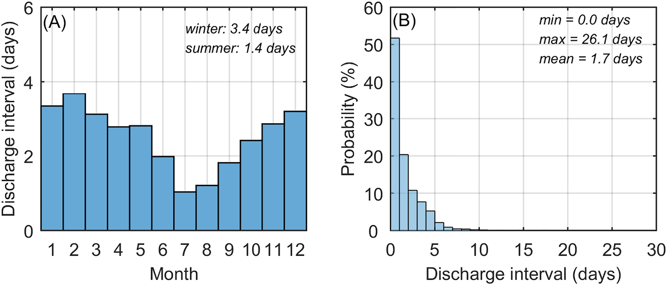
Figure 1 Interval between freshwater discharges from Geum River estuarine dam during 1994-2016. (A) Long term average discharge interval by month, (B) discharge interval probability distribution. Winter is December – February and summer is July – September. Data provided by the Korea Rural Community Corporation.

There is little existing research on the effect of dam location and discharge interval on estuaries. Zhu et al. (2017) analyzed depositional patterns in the Xinyanggang estuary, China (dam at x = 10 km), using a numerical model. Dam locations at x = 1 and 6 km and discharge intervals of Δt = 1 – 7 days were investigated. It was found that longer channels favored enhanced siltation due greater flood-dominance, and more frequent discharge reduced siltation. Schuttelaars et al. (2013) analyzed sediment trapping in the Ems estuary, Germany (weir at x = 60 km), using an idealized analytical model. Weir locations between x = 20 – 100 km were investigated. It was found that the weir was near resonance and relocating the weir landward away from resonance could reduce the tidal asymmetry and shift the sediment trapping location seaward. Together these two papers established that the estuarine dam location can strongly affect the tidal asymmetry and sediment trapping. With respect to the discharge interval, Azevedo et al. (2010) analyzed the effect of river discharge patterns in the Douro estuary, Portugal (dam at x = 22 km). It was found that variable discharges were less effective at flushing salt and dispersing contaminants compared to steady discharge. This indicates that the discharge interval can control the estuarine salinity and contaminants in addition to sediment transport reported by Zhu et al. (2017).

As these research studies focused primarily on strongly tidal systems, less research has been conducted on the effect of estuarine dam location in different estuarine types, such as partially mixed or strongly stratified estuaries. Furthermore, the effect of the discharge interval doesn’t appear to have been studied for estuarine dams located further than about x = 20 km from the mouth. Therefore, this study was carried out to extend the results of Figueroa et al. (2022), which investigated the effect of an estuarine dam on estuarine types, to include the effect of the estuarine dam location and discharge interval. The overall objective of this study is to understand the effect of estuarine dam location and discharge interval on estuarine processes. Specific research questions are: 1) how does the estuarine dam location affect the tidal processes?, 2) how does the discharge interval affect the river processes?, 3) how do changes in tidal and river processes affect the salinity and estuarine classification?, and 4) how do changes in tidal and river processes affect the sediment transport and estuarine morphology?

To address these research questions, an idealized numerical model of strongly stratified, partially mixed, periodically stratified, and well-mixed estuaries was used. Estuarine dams were placed in the region of the salt intrusion at x = 20, 55, and 90 km, and the discharge interval was varied from the tidal to the spring-neap cycle timescales at Δt = 0.5, 3, and 7 days. After evolving for one year, both the pre- and post-dam results were compared based on changes in hydrodynamic, sediment dynamic, and morphodynamic processes. Then trends in the response to the estuarine dam for each estuarine type, dam location, and discharge interval were analyzed.

This paper is organized as follows. Section 2 describes data collection and processing. Section 3 presents the results in order of changes to tide and river processes, salinity related processes and estuarine classification, and sediment flux mechanisms and depth change. Section 4 discusses the interaction of the estuarine dam location and discharge interval with estuarine spatial and temporal scales, the implications of this study for coastal hazards, and the reliability of the idealized estuary model. Finally, Section 5 summarizes the key findings.

2 Materials and methods

2.1 Data collection

2.1.1 Model description

This study used the ocean and sediment transport models of the Coupled-Ocean-Atmosphere-Wave-Sediment Transport (COAWST) modeling system (Warner et al., 2010). The ocean model is the Regional Ocean Modeling System (ROMS) which is a free surface, terrain-following numerical model that solves the three-dimensional Reynolds averaged Navier-Stokes equations using the hydrostatic and Boussinesq approximations (Haidvogel et al., 2008). The sediment transport model is the Community Sediment Transport Modeling System (CSTMS) which computes suspended sediment transport using the advection-diffusion algorithm together with an additional algorithm for vertical settling (Warner et al., 2008; Warner et al., 2010).

2.1.2 Model domain

Figure 2 shows the model domain used for scenarios with no estuarine dam and for scenarios with an estuarine dam at x = 20, 55, and 90 km. From the estuary mouth, the pre-dam domain extends 25 km seaward representing a shelf and 250 km landward representing an estuary and tidal river. The idealized estuary is funnel shaped near the mouth but becomes straight 5 km landward of the mouth. The depth decreases linearly and is constant after 90 km from the mouth. The dam location at x = 20 km was based on statistics of real estuaries with estuarine dams (Figueroa et al., 2022). The dam location at x = 90 km was selected as it is the location furthest inland before the depth transition (Figure 2D). The location at x = 55 km was chosen as it is the midpoint between these. The across-channel shape is Gaussian. The pre-dam domain had an along-channel, across-channel, and vertical discretization of 242 × 62 × 20 points. The model was run with a 5 s baroclinic time step, which was divided into 20 barotropic time steps. For each post-dam scenario, the portion of the domain upstream of the estuarine dam was removed.

FIGURE 2

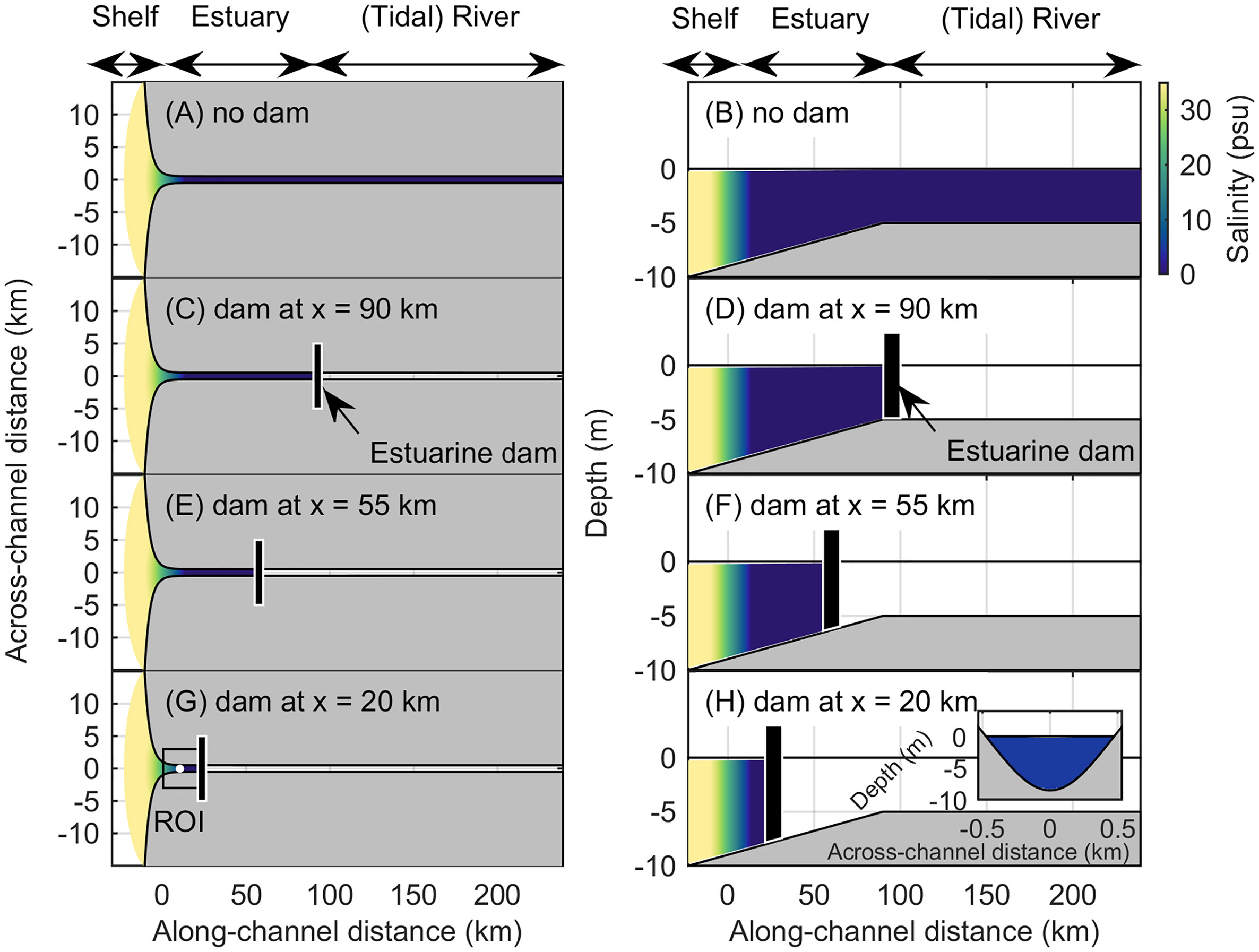
Figure 2 Model domain for (A, B) no dam, (C, D) dam at x = 90 km, (E, F) dam at x = 55 km, and (G, H) dam at x = 20 km scenarios. Left plots are top-view, right plots are side-view. Salinity and bathymetry are the model initial conditions. An example of a region of interest (ROI) for a post-dam estuary shown in (G). Point is the ROI center and is the location of the across-channel transect shown as an inset in (H) and the Figure 6 time series.

2.1.3 Model setup and boundary conditions

Table 1 lists the sediment properties for the six non-cohesive size classes used. These were divided into two groups: a marine sediment group (sand_1, mud_1, and mud_2) and a fluvial sediment group (sand_2, mud_3, and mud_4), which had the same properties. The model was initialized with only marine sediments well-mixed in the domain bed. Fluvial sediments were discharged from the river and estuarine dam to investigate the mixing of marine and fluvial sediments. During the runs the bed was allowed to evolve, resulting in morphodynamic change. This included intertidal areas which were included by a wetting and drying scheme.

TABLE 1

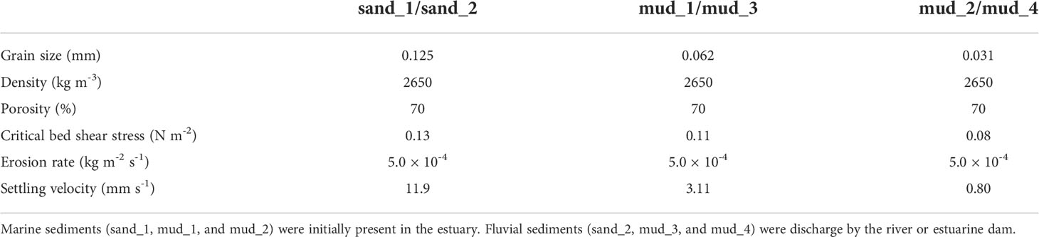
Table 1 Sediment properties.

The boundary conditions were closed on the channel banks and river end. The ocean boundary was open and featured a Chapman implicit boundary condition for the free surface and a Flather condition for the 2D momentum. The free surface and 2D momentum boundary conditions on the ocean boundary were chosen such that tidal currents were calculated from the free surface using reduced physics. Radiation and nudging conditions were applied to the salinity and sediment tracers such that they could radiate from the domain at the ocean boundary. The salinity and suspended sediment concentration (SSC) at the ocean boundary were defined as 35 psu and 0 kg m^-3, respectively.

On the river boundary, a constant river discharge was imposed for the pre-dam cases. For the post-dam cases, the discharge points were relocated to the estuarine dam, and the discharge became episodic to simulate estuarine dam operation. Discharge events from the estuarine dam were limited to 3 hours around mid-ebb tide, when the flow is seaward. During flood tides, the sluice gates are closed to block upstream salt intrusion. While dam operation may vary between estuaries with estuarine dams, this operation of discharges only during ebbs or low tides is known to occur in several estuaries including Dutch (Ye, 2006; Nauw, 2014), French (Laffaille et al., 2007; Traini et al., 2015), Chinese (Zhu et al., 2017), and Korean (Shin et al., 2019) estuaries.

2.1.4 Model scenarios

Table 2 lists the model scenarios which are organized based on estuarine type, dam location, and discharge interval. The estuarine types are the strongly stratified (hereinafter SS), partially mixed (hereinafter PM), periodically stratified (hereinafter PS), and well-mixed (hereinafter WM) estuaries. The freshwater discharge varied from continuous (no dam) to discrete discharge intervals of Δt = 0.5, 3, and 7 days. These discharge intervals were selected to examine the interaction of the freshwater discharge with the tidal and spring-neap cycles. The post-dam freshwater discharge was scaled with the discharge interval to ensure the volume of discharged water over a spring-neap cycle was same for the pre- and post-dam estuaries. This assumes that the reservoir of the estuarine dam is not limited and thus the discharge interval is determined a priori (i.e., by a dam operator).

TABLE 2

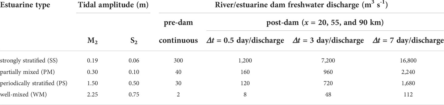
Table 2 Model scenarios.

For each estuarine type and discharge interval, the dam location was varied as x = 20, 55, and 90 km. For convenience, hereinafter a scenario is denoted as, for example, ${\text{PM}}_{90}^{0.5}$, where the subscript denotes the dam location and the superscript denotes the discharge interval. The set of scenarios for the partially mixed estuary can then be written as PM, ${\text{PM}}_{20}^{0.5}$, ${\text{PM}}_{20}^3$, ${\text{PM}}_{20}^7$, ${\text{PM}}_{55}^{0.5}$, ${\text{PM}}_{55}^3$, ${\text{PM}}_{55}^7$, ${\text{PM}}_{90}^{0.5}$, ${\text{PM}}_{90}^3$, ${\text{PM}}_{90}^7$, where no super or subscript denotes the pre-dam estuary. Thus, 10 scenarios were implemented for each estuarine type resulting in a total of 40 simulations (4 pre-dam and 36 post-dam). To refer to a group of results, the super and subscripts are written using variables. For example, ${\text{PM}}_{\text{x}}^{0.5}$ denotes all partially mixed estuaries with a discharge interval of Δt = 0.5 days, and ${\text{PM}}_{90}^{\Delta t}$ denotes all partially mixed estuaries with a dam location of x = 90 km. For convenience, the SS and PM estuaries are also referred to as “river-dominated” end members and the PS and WM estuaries are also referred to as “tide-dominated” end members based on their dominant forcing.

For the pre-dam scenarios, a salinity initialization was implemented followed by a 365-day pre-dam model run. For the post-dam scenarios, the salinity, bed morphology, SSC, and so forth of the pre-dam run were used as the initial condition for the post-dam run and the model was run for an additional 365 days. Data in the estuarine region of the domain and for a selected spring-neap cycle at the end of the runs constitute the dataset of this study. For more information on the model setup and workflow the reader is referred to Figueroa et al. (2022).

2.2 Data processing

To understand the effect of dam location and discharge interval on estuarine hydrodynamics, sediment dynamics, and morphodynamics several analysis methods were employed and are described here. Note, for the purpose of this study, key trends from these analyses are highlighted using selected model scenarios. For processed data from all model scenarios, the reader is referred to the Supplementary Material.

2.2.1 Tide and current amplitude and phase

Tide and current amplitude and phase were extracted along-channel for the principal lunar semidiurnal constituent (M₂) for all scenarios using classical tidal harmonic analysis (Pawlowicz et al., 2002). This allowed the analysis of amplification or damping of tides and currents as well as change in the relative phase between current and tide. When interpreting the phase difference, a phase difference of 0° of denotes a progressive wave, a phase difference of 90° of denotes a standing wave, and an intermediate phase difference denotes a mixed wave.

To check the numerical results of change in tidal dynamics, an analytical model of tidal propagation in estuaries with and without an estuarine dam (Cai et al., 2016) was implemented and compared with the numerical results. The analytical model is essentially a function which takes inputs of channel characteristics and tides at the mouth and outputs the along-channel variation of the tidal amplitude, velocity amplitude, and the phase difference between velocity and tide. For simplicity, a straight channel with no tidal flats was specified. The best calibration of the data was found to occur for a Manning-Strickler friction coefficient of K = 65 m^1/3 s^-1 and was applied equally to all scenarios.

2.2.2 Mean sea level and Eulerian residual current

In addition to higher frequency tidal hydrodynamics, lower frequency sea level and Eulerian residual current were analyzed. In particular the Eulerian residual current has important implications for sediment and morphodynamics. The along-channel variation of mean sea level and Eulerian residual currents were obtained from the model by spring-neap averaging. To better understand the driving processes, two processes were considered. First is the water setup due to freshwater input and the seaward river runoff. The cross-sectionally averaged runoff, U_R, was calculated from the model as:

$\begin{array}{ll}{\text{U}}_{\text{R}}=V/A& (1)\end{array}$

where V is the freshwater discharge and A is the channel cross-sectional area. Second was the landward Stokes drift (a Lagrangian current), Stokes water setup, and the seaward Stokes return flow (an Eulerian current). In strongly tidal estuaries with progressive or mixed tides, a landward Stokes drift is generated due to correlations between the vertical and horizontal tides. The Stokes drift can be approximated by (Uncles and Jordan, 1980; Guo et al., 2014; Moftakhari et al., 2016):

$\begin{array}{ll}{U}_{stokes}=\frac{1}{2}av\cos \left(\phi \right)/h& (2)\end{array}$

where a is the tidal amplitude, v is the velocity amplitude, ϕ is the relative phase, and h is the water depth. Over the spring-neap cycle, the landward Stokes drift and seaward Stokes return flow are balanced, and Eq. 2 can be used to estimate the seaward Stokes return flow (Eulerian residual current). The output of a, v, and ϕ from the tidal harmonic analysis for the M₂ tidal constituent was used to evaluate Eq. 2 for each scenario.

2.2.3 Tidal asymmetry

In addition to the Eulerian residual currents, tidal asymmetry is also an important factor for estuarine sediment and morphodynamics. Guo et al. (2019) reviewed two methods of quantifying tidal asymmetry, namely the harmonic and statistical methods. The harmonic method follows Friedrichs and Aubrey (1988) quantifying the tidal asymmetry via:

$\begin{array}{ll}{M}_4/M_2 =v_{M4}/v_{M2}& \text{(3a)}\end{array}$

$\begin{array}{ll}2{\text{M}}_2-{\text{M}}_4=2{\text{θ}}_{\text{M}2}-{\theta }_{M4}& \text{(3b)}\end{array}$

where M₄ is the shallow water overtide of the M₂ tidal constituent. Eq. 3a is the ratio of the M₄ and M₂ velocity amplitudes, and its magnitude denotes the magnitude of the tidal asymmetry. Eq. 3b is the phase difference between the M₂ and M₄ velocity constituents, and it determines the direction of the tidal asymmetry. For −90°< 2θ_M2−θ_M4<90° , the tide is flood-dominant, and for 90°<2θ_M2−θ_M4<270° , the tide is ebb-dominant. For scenarios of this study, the amplitude ratios (Eq. 3a) were averaged over the remnant estuaries and normalized by the corresponding pre-dam values to detect global changes in asymmetry magnitude. The phase difference (Eq. 3b) was also averaged over the remnant estuaries to detect global changes in asymmetry direction. To facilitate comparison between scenarios, the value of the phase difference was set to a binary -1 or +1 to denote either ebb-dominance or flood-dominance, respectively.

The harmonic method works well to understand tidal asymmetry due to distortion of the tidal wave due to frictional interaction with the bottom and intertidal storage. Another form of tidal asymmetry can occur when a tidal current is superimposed on an Eulerian residual current, known as Euler-induced asymmetry (Guo et al., 2014). The harmonic method does not include the Eulerian residual, however the statistical method to quantify tidal asymmetry can. The statistical method follows Nidzieko (2010) and Nidzieko and Ralston (2012) quantifying the tidal asymmetry via a velocity skewness parameter, γ₁, as:

$\begin{array}{ll}{\gamma }_1=\frac{{\mu }_3}{{\sigma }^3}=\frac{\frac{1}{\tau -1}{\sum }_{t=1}^{\tau }{\left(v_b\right)}^3}{{\left[\frac{1}{\tau -1}{\sum }_{t=1}^{\tau }{\left(v_b\right)}^2 \right]}^{\frac{3}{2}}}& (4)\end{array}$

where µ₃ is the third sample moment, σ is the standard deviation, v_b is the bottom current. To investigate the Euler-induced asymmetry, µ₃ and σ were taken about zero and not the mean. The bottom current was used as it is important for the sediment transport. The summation is for τ observations from time t = 1 to t = τ. The magnitude of the velocity skewness indicates the magnitude of tidal asymmetry and the sign indicates the direction (γ₁< 0 is ebb-dominant and γ₁ > 0 is flood-dominant) To facilitate comparison between scenarios, the value of the velocity skewness was also set to a binary -1 or +1 to denote either ebb-dominance or flood-dominance, respectively.

2.2.4 Discharge pulse, baroclinic processes, and exchange flow

Discharge of freshwater from an estuarine dam into an estuary results in a seaward propagating pulse of freshwater which decreases in magnitude with distance (Figueroa et al., 2020a; Figueroa et al., 2020b). The pulse speed and range of influence are important factors relevant to salinity and sediment transport. To quantify the high frequency freshwater discharge forcing along-channel (in contrast to low frequency, Section 2.2.2.), time series were selected along-channel, and height of jumps in water level and velocity, associated with the pulse front, were manually extracted.

To better understand the effect of the estuarine dams on the baroclinic hydrodynamics and associated sediment dynamics, spring-neap averaged along-channel salinity and stratification data were collected for each scenario. For the same reason, the following measure for the intensity of the estuarine exchange flow was used based on a similar measure used by Burchard and Hetland (2010):

$\begin{array}{ll}\mu (\langle u\rangle )={\displaystyle {\int }_0^1\left|\langle u\left(\sigma \right)\rangle \right|}d\sigma & (5)\end{array}$

where μ is referred to here as an exchange flow parameter, u is a spring-neap average velocity profile, and σ is the nondimensional sigma depth (σ = z/h, z is vertical coordinate, h, is water depth) ranging from zero at the bed to one at the surface. The parameter μ calculates the average absolute value of a residual velocity profile. If there was not a residual two-layered circulation, μ was set to zero.

2.2.5 Estuarine parameter space

Previous analyses were directed at understanding changes in tide and river processes caused by an estuarine dam. Such changes in turn may affect the estuarine type which has implications for both the post-dam hydrodynamics and sediment dynamics. To quantify changes in the estuarine type, the estuarine parameter space was used based on the freshwater Froude number, Fr_f, and the mixing number, M, defined as (Geyer and MacCready, 2014):

$\begin{array}{ll}F{r}_f=\frac{U_R}{{\left(\beta g{S}_{ocean}H\right)}^{\frac{1}{2}}}& \text{(6a)}\end{array}$

$\begin{array}{ll}{M}^2=\frac{C_D{U}_T^2}{\omega N_0{H}^2}& \text{(6b)}\end{array}$

where U_R is the cross-sectionally averaged river discharge velocity, H is the cross-sectionally averaged depth, U_T is the amplitude of the cross-sectionally averaged tidal velocity, N₀ = (βgS_ocean/H)^1/2 is the buoyancy frequency for maximum bottom-to-top salinity variation in an estuary, β = 7.7 × 10^-4 psu^-1 is the coefficient of haline contraction, S_ocean = 35 psu is the ocean salinity, g = 9.8 m s^-2 is the acceleration due to gravity, C_D (taken here as C_D = 2.5 × 10^-3) is the drag coefficient, and ω = 1.4 × 10^-4 s^-1 is the tidal frequency.

Physically, Fr_f is the net velocity of the river flow scaled by the maximum possible frontal propagation speed, and M is the ratio of tidal timescale to the mixing timescale (Geyer and MacCready, 2014). To keep the points within the parameter space for the post-dam estuaries, minimum values of M = 0.22 and Fr_f = 1.5 × 10^-4 and a maximum value of Fr_f = 0.9 were specified. Physically, these represent very low currents, very low freshwater discharge, and very high freshwater discharge approaching the maximum baroclinic frontal propagation speed, respectively. It is noted that, in contrast to Figueroa et al. (2022), this study allows U_T to include currents due to the discharge pulse from the estuarine dam, thus permitting the dam discharge to affect M.

2.2.6 Sediment flux decomposition and bathymetric and surficial sediment change

Changes in hydrodynamics can induce changes in sediment and morphodynamics. Several processes affect both the sediment and morphodynamics. Sediment accumulation and estuarine turbidity maximum (ETM) formation are due to the convergence of tidally averaged, cross-sectionally integrated suspended sediment transport, A[uc]_A. To highlight the relevant underlying processes, the sediment fluxes were decomposed following Burchard et al. (2018):

$\begin{array}{ll}\langle A{\left[uc\right]}_A\rangle =\underset{T}{\underbrace{W{\left[\langle D{\left[uc\right]}_z\rangle \right]}_y}}=\underset{T_a}{\underbrace{W{\left[\langle D\rangle {\langle \left[u\right]}_z\rangle {\langle \left[c\right]}_z\rangle \right]}_y}}+\underset{T_b}{\underbrace{W{\left[\langle D\rangle \langle \left[u\right]{\text{'}}_z\left[c\right]{\text{'}}_z\rangle \right]}_y}}+\underset{T_c}{\underbrace{W{\left[\langle D\rangle {\left[\langle \tilde{u}\rangle \langle \tilde{c}\rangle \right]}_z\right]}_y}}+\underset{T_d}{\underbrace{W{\left[\langle D\rangle {[\langle \tilde{u}\text{'}\tilde{c}\text{'}\rangle ]}_z\right]}_y}}+\underset{T_e}{\underbrace{W{[\langle D^{\prime }\left[uc\right]{\text{'}}_z\rangle ]}_y}}& (7)\end{array}$

where u is the along-channel current velocity, c is the suspended sediment concentration, D is the depth, W is the width, and A is the cross-sectional area. Here, [·]_y, [·]_z, and [·]_A denote lateral, vertical, and cross-sectional averages, respectively, and 〈·〉 denotes a tidal average. The prime (‘) denotes the deviation from a tidal average and a tilde (~) denotes the deviation from a vertical mean. In this way the temporally averaged, cross-sectionally integrated transport was decomposed into five terms, T_a - T_e. Each term is associated with a different sediment transport mechanism. T_a is the transport by averages often due to down-estuary river runoff. T_b is the tidal covariance transport due to tidal pumping. T_c is the vertical covariance of tidal averages transport due to the estuarine exchange flow. T_d is the combined vertical and temporal covariance transport, e.g. suspended sediment is mixed higher up into the water during flood than during ebb by tidal straining. And T_e is the temporal depth covariance transport due to Stokes transport.

The terms were quantified along-channel in both the pre- and post-dam cases to understand the impact of the estuarine dam on the sediment flux mechanisms. As Eq. 7 is exact only for constant depth or averaging in depth-proportional sigma coordinates (Burchard et al., 2018), averaging was done in sigma coordinates. The operations 〈·〉 for a tidal average and (‘) for a deviation from a tidal average were computed using Lanczos 36-hour low-pass and high-pass filters, respectively. To facilitate identifying changes between scenarios, T_a - T_e were averaged over representative pre- and post-dam spring-neap cycles, turning them into a function of only along-channel position. To quantify associated changes in the SSC, morphology, bed mud fraction, and bed fluvial sediment fraction, representative width-averaged along-channel transects were obtained from the model for all scenarios.

3 Results

3.1 Effect of estuarine dam location on tidal processes

The effect of the discharge interval on tidal processes was found to be minor in comparison with the location of the estuarine dam. Therefore, this section uses the post-dam scenarios with the discharge interval Δt = 3 days and focuses on the effect of estuarine dam location.

3.1.1 Tide and current amplitude and phase

Figure 3 presents numerical and analytical pre- and post-dam along-channel profiles of M₂ tidal amplitude, current amplitude, and phase difference between current and tide depending on the estuarine dam location. Considering first the numerical result, the tidal amplitude (Figures 3A1-D1) increased for all post-dam estuaries. In the pre-dam estuaries, the tidal amplitude was constant along-channel for the river-dominated estuaries and decreased landward in the tide-dominated estuaries due to friction. In the post-dam estuaries, the tides increased landward for dam locations x = 20 and 55 km due to reflection of the tidal wave. For dam location x = 90 km, the tidal amplitude near the mouth decreased landward due to friction before increasing near the dam due to reflection. The analytical and numerical results generally matched well. However, it was noted that for the tide-dominated estuaries, post-dam changes in the bathymetry needed to be considered. Thus, without accounting for the post-dam deepening of the mouth from about 6.5 m to 8 m (Section 3.4. below), the post-dam tidal amplitudes were underestimated (Figures 3C1-D1).

FIGURE 3

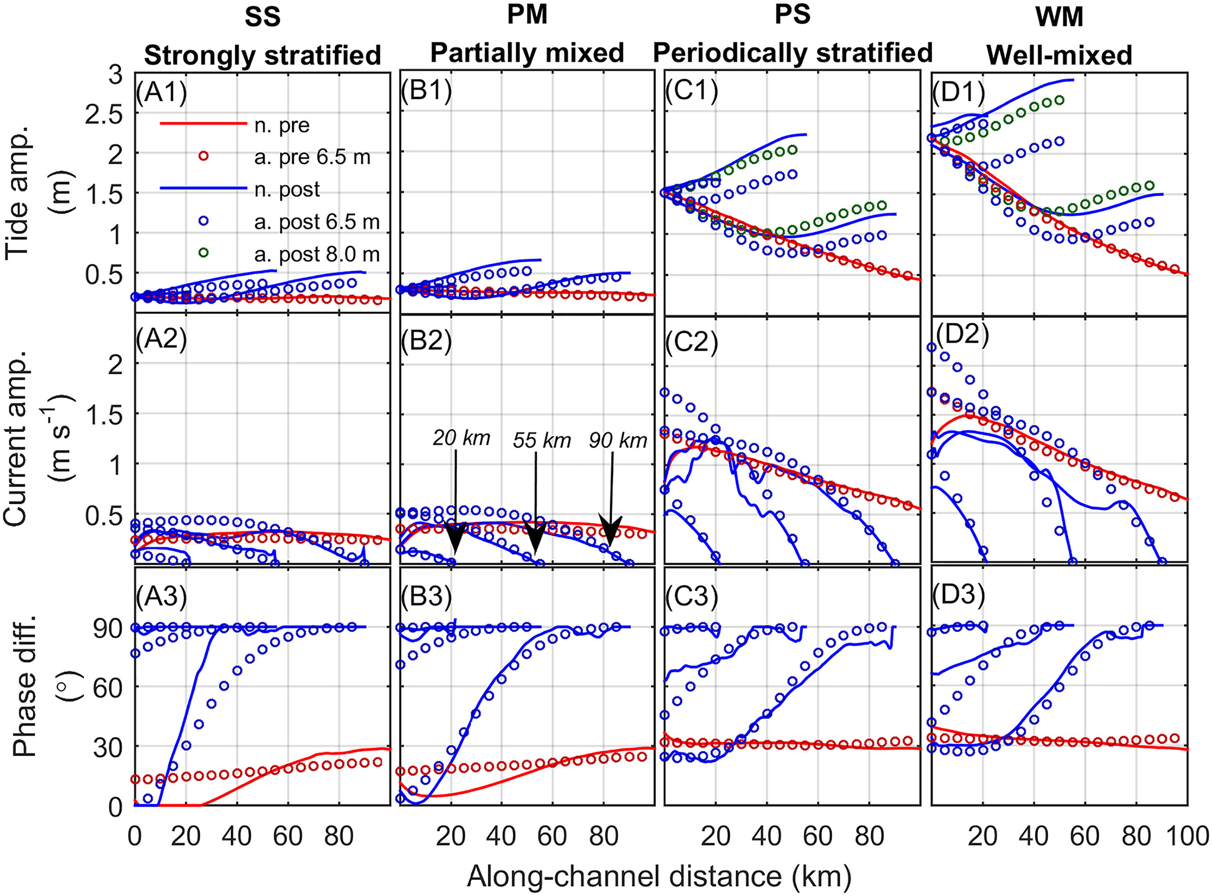
Figure 3 Pre- and post-dam along-channel profiles of (A1-D1) M₂ tidal amplitude (m), (A2-D2) M₂ current amplitude (m s^-1), and (A3-D3) phase difference between current and tide (°) depending on estuarine dam location (dam at x = 20, 55, and 90 km). Along-channel is distance is from the estuary mouth, positive landward. n. is numerical, a. is analytical, pre is pre-dam, post is post-dam, and 6.5 m and 8.0 m represent the depth at the estuary mouth used in the analytical model. Most analytical models used 6.5 m. All results correspond to scenarios with discharge intervals Δt = 3 days.

Figures 3A1-D1 support numerically that for a given tidal constituent (here M₂) a particular dam location can cause maximum tidal amplification due to resonance. For a frictionless, non-convergent estuary, the resonance length is well known to occur when the channel length is a quarter of the tidal wavelength. A simple estimate of the tidal wavelength, L, using $L=T\sqrt{gh}$ with tidal period T = 12.4 hr, acceleration due to gravity g = 9.8 m s^-2, and water depth h = 6.5 m gives L = 360 km and thus a resonance length of L/4 = 90 km. This is greater than the resonance length evident in Figure 3D1 where maximum amplification based on the available data occurs near x = 55 km. This is because friction acts to reduce the resonance length. Unfortunately, in the frictional case an explicit analytical solution for the resonance length cannot be found because it requires an iterative procedure (Cai et al., 2016). However, based on the iterative procedure, (Cai et al., 2016; their Figure 7) plotted the resonance length for the frictional case in the estuary shape number (γ, representing the effect of cross-sectional area convergence) – friction number (x, describing the role of the frictional dissipation) space. Using the WM estuary as an example, γ = 0 (straight channel) and x = 2.5 (moderate to strong friction) and the resonance length is estimated approximately as L/8 = 45 km, which is similar to the numerical result. It is noted that the resonance length depends on the tidal amplitude through the friction number, and therefore for a straight channel, smaller tidal amplitudes will have smaller friction numbers, and their resonance lengths will approach the classical L/4. This is the case in Figure 3A1 where the resonance length in the microtidal SS estuary is likely closer to L/4 = 90 km.

The along-channel current amplitude decreased for the post-dam estuaries (Figures 3A2-D2). All post-dam estuaries exhibited currents vanishing at the estuarine dam due to the dead-end channel. The dam location at x = 90 km caused the least change compared to pre-dam conditions, and the dam location at x = 20 km caused the greatest reduction in tidal currents. This was due to the loss of tidal prism near the mouth. For dam locations at x = 55 km in the region of the resonance length, the analytical model predicted larger currents at the mouth. The numerical model did not show these large currents likely due to morphological adjustment (i.e., deepening of the mouth, Section 3.4.).

The pre-dam estuaries had phase differences ranging from φ = 0 - 30°, indicating a progressive and mixed wave character. Considering the WM estuary as an example, this estuary can be classified following Friedrichs (2010) as a long, intermediate depth, nonconvergent estuary. For this case, the e-folding length of the along-channel tidal amplitude, L_a, can be used to analytically estimate the phase difference as $\text{φ}=\text{arctan}\left({\text{L}}_{\text{a}}^{-1}/k\right)$, where k is the tidal wavenumber. Using data from the WM estuary yields a phase difference estimated analytically as φ = 40°. This is similar to the numerical result and indicates that the pre-dam estuaries lie between progressive (φ = 0°) and diffusive tides (φ = 45°).

The post-dam estuaries show a shift to standing wave phase difference (φ = 90°) due to wave reflection. Dams located near the mouth (x = 20 km) changed the entire remnant estuary to have a standing wave character. Dams located near the resonance length and landward of the resonance length had progressive or mixed tides at the mouth and standing waves near the estuarine dam (x = 55 and 90 km). The analytical result agreed well with the numerical result. For dam locations beyond the resonance length, the distance from the reflecting end where the reflected wave influences the estuary was given by Friedrichs (2010). The reflected wave should be included for distances less than about |L_a|/2, where |L_a| is the absolute value of L_a as predicted by:

$\begin{array}{ll}\frac{{\text{L}}_{\text{a}}^{-1}}{k}=\frac{\omega }{r}-{\left(\frac{{\omega }^2}{r^2}+1\right)}^{1/2}& (8)\end{array}$

where r = 8c_DU/3πh is the friction factor, c_D is the drag coefficient, U is the tidal amplitude, and h is the tidally averaged depth. Taking the WM estuary as an example, the distance from the estuarine dam where the reflected wave influences the estuary is found to be about 40 km, which agrees with the model result where the tides transition from a mixed to standing wave character (Figure 3D3).

3.1.2 Mean sea level and Eulerian residual current

The pre- and post-dam mean sea levels and Eulerian residual currents were different for the river-dominated estuaries (particularly the SS estuary) and the tide-dominated estuaries (PS and WM; Figure 4). For the river-dominated estuaries, the pre-dam mean sea levels increased landward due to the freshwater discharge (Figures 4A1-B1). For the PM estuary, the post-dam mean sea levels were similar, but they increased considerably for the post-dam SS estuary because it had the largest input of freshwater volume during a discharge event which was enough to increase the spring-neap averaged sea level. The Eulerian residual currents were seaward (Figures 4A2-B2) and due to river runoff with negligible Stokes return flow (Figures 4A3-B3). The estuarine dam resulted in partially reduced seaward Eulerian currents due to scour of the channel adjacent to the dam (Section 3.4.) and the change from continuous to episodic freshwater discharge. The dam location did not change the overall trend in post-dam mean sea level and Eulerian residual current in the river-dominated estuaries.

FIGURE 4

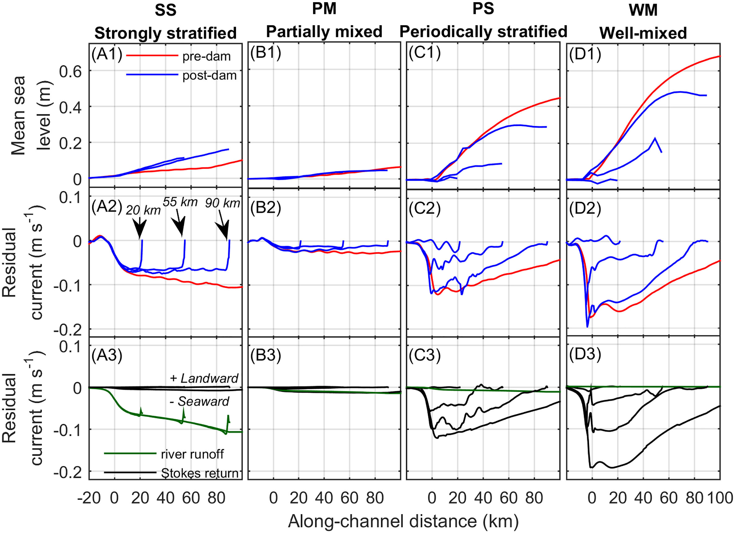
Figure 4 Pre-dam and post-dam along-channel profiles of (A1-D1) mean sea level (m), (A2-D2) cross-sectionally averaged Eulerian residual currents (m s^-1), and (A3-D3) river runoff (m s^-1) and Stokes return flow (m s^-1) depending on estuarine dam location (dam at x = 20, 55, and 90 km). Along-channel distance is distance from the estuarine mouth, positive landward. Negative current is seaward. All results correspond to scenarios with discharge intervals Δt = 3 days.

For the tide-dominated estuaries, the pre-dam mean sea levels increased landward due to the mixed tides generating a landward Stokes drift and water level setup (Figures 4C1-D1). As the dam location moves toward the mouth, a greater proportion of the estuary experiences standing wave tides, and the landward Stokes drift, Stokes setup (Figures 4C1-D1), and Stokes return flow (Figures 4C2-D2) are reduced. Analytic expressions supported that the Stokes return flow was the main process contributing to the Eulerian residual current and river runoff was negligible (Figures 4C3-D3). Thus, the dam location was found to have a strong effect on the mean sea level and Eulerian residual currents in the tide-dominated estuaries. Furthermore, the effect was greatest for the estuarine dam location near the mouth (x = 20 km). This has important ramifications for the transport of sediment by the Eulerian residual current as well as the Euler-induced tidal asymmetry.

3.1.3 Tidal asymmetry

Change in tidal asymmetry for different estuarine types and dam locations is shown in Figure 5. Based on the harmonic method, the magnitude of tidal asymmetry stayed the same or increased for almost all post-dam estuaries (Figure 5A). Relative to the pre-dam tidal asymmetry, the magnitude of the post-dam tidal asymmetry increased the most for the river-dominated estuaries likely due to their pre-dam tides being relatively small, and thus small changes have a relatively larger effect. The dam location near resonance (x = 55 km) caused the least change in tidal asymmetry magnitude whereas the dam location near the mouth (x = 20 km) changed the most. These changes were likely because of differential amplification of the M₂ and M₄ constituent, changes in mean sea level, and morphologic change. Based on the harmonic method, the tidal asymmetry direction for the river-dominated estuaries was mostly ebb-dominant and for the tide-dominated estuaries was mostly flood-dominant (Figure 5B). This agrees with Friedrichs and Aubrey (1988) who identified that increasing tidal range promotes flood-dominance.

FIGURE 5

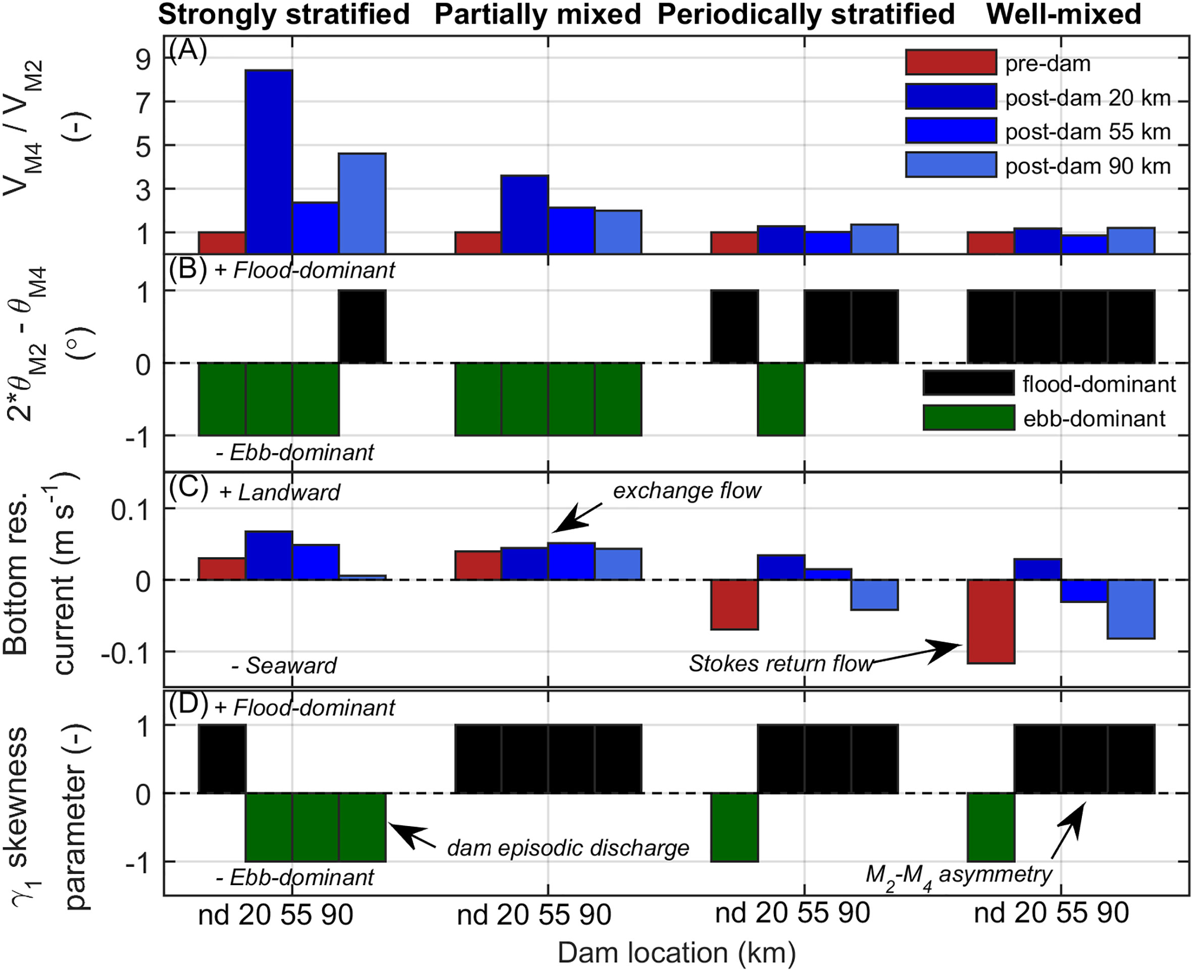
Figure 5 Pre- and post-dam tidal asymmetry for different dam locations and estuarine types. (A) Ratio of M₄ to M₂ tidal constituent velocity amplitude (v_M4/v_M2, -) with values normalized to each type’s pre-dam case, (B) M₂ and M₄ tidal constituent velocity relative phase difference (2θ_M2 – θ_M4, °) binned based on dominance, (C) bottom residual currents (m s^-1), and (D) bottom velocity skewness parameter (γ₁, -) with values binned based on dominance. The no dam case is denoted nd. All results correspond to scenarios with discharge intervals Δt = 3 days.

To discuss the tidal asymmetry based on the statistical method and the Euler-induced tidal asymmetry, the bottom Eulerian residual current is shown for reference in Figure 5C. For the pre-dam river-dominated estuaries, the estuarine exchange flow was the main process, and it drove an upstream bottom Eulerian residual current. For the pre-dam tide-dominated estuaries, the Stokes return flow was the main process, and it drove a seaward bottom Eulerian residual current. The post-dam river-dominated estuaries maintained an upstream Eulerian residual current. In the post-dam tide-dominated estuaries, the switch from mixed to more standing wave tides caused the Stokes return flow to be reduced ($P{S}_{90}^3$, $W{M}_{55}^3$, $W{M}_{90}^3$) or replaced by landward exchange flow ($P{S}_{20}^3$, $P{S}_{55}^3$, $W{M}_{20}^3$). Based on the velocity skewness, the tidal asymmetry direction tended to match the bottom Eulerian residual current (indicating Euler-induced asymmetry) with two exceptions. First were $S{S}_{20}^3$, $S{S}_{55}^3$, and $S{S}_{90}^3$ where the velocity skew was dominated by the high frequency freshwater discharge events rather than the low frequency Eulerian residual currents. Second were $P{S}_{90}^3$, $W{M}_{55}^3$, and $W{M}_{90}^3$ where the effect of tidal distortion and interaction of the M₂ and M₄ constituents was greater than the Euler-induced tidal asymmetry caused by the Stokes return flow. Overall, these results highlight the importance of Euler-induced tidal asymmetry and also the dam episodic discharge in the post-dam SS estuary and interaction of the M₂ and M₄ constituents in the post-dam tide-dominated estuaries.

3.2 Effect of estuarine dam discharge interval on river processes

3.2.1 Sea surface elevation, current, salinity, and SSC time series

As freshwater discharges are events, time series comparing river- and tide-dominated end members under different discharge intervals is shown in Figure 6. Here, data of $S{S}_{20}^{\Delta t}$ and $W{M}_{20}^{\Delta t}$ from the center of the post-dam estuary were selected (center of region of interest, ROI, see Figure 2G).

FIGURE 6

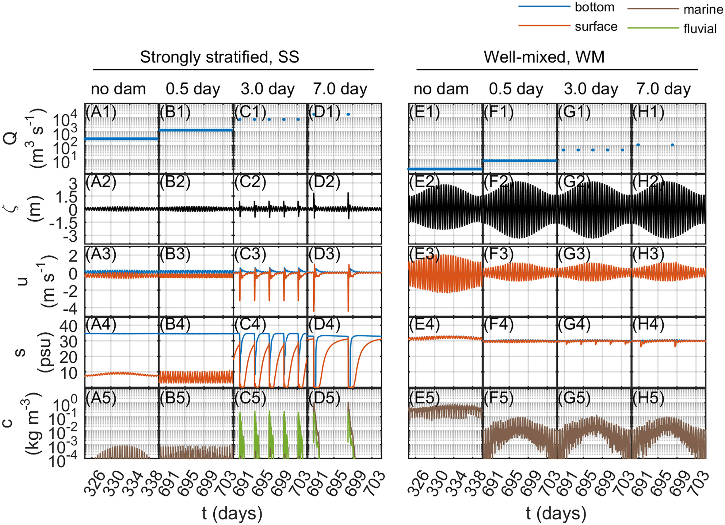
Figure 6 Representative time series comparing strongly stratified and well-mixed estuaries under different discharge intervals. (A1-H1) Freshwater discharge (Q, m³ s^-1), (A2-H2) sea surface elevation (ζ, m), (A3-H3) bottom and surface along-channel current velocity (u, m s^-1); (A4-H4) bottom and surface salinity (s, psu), and (A5-H5) suspended sediment concentration (c, kg m^-3) versus time (t, days). Data are from the center of the region of interest (ROI) for cases with an estuarine dam at x = 20 km. Time is day since initialization with estuarine dam placed on day 365. Positive velocity is landward.

In the pre-dam SS estuary, the discharge was continuous, the tidal range was small, a distinct two-layer circulation occurred, the estuary was strongly stratified, and sediment was resuspended during the spring tides (Figures 6A1-A5). The $S{S}_{20}^{0.5}$ estuary was overall similar with some change in the surface salinity and bottom resuspension due to discharges during ebb (Figures 6B1-B5). Once the discharge interval exceeded the tidal cycle period, the response was different. The $S{S}_{20}^3$ estuary had increasingly spaced discharge periods (Figure 6C1). The greater freshwater volume per discharge resulted in a noticeable water level set up, seaward current pulse, freshwater frontal propagation, and greater resuspension of bottom marine sediment and advection of fluvial sediment (Figures 6C2-C5). The $S{S}_{20}^7$ estuary was similar to the $S{S}_{20}^3$, but the magnitude of the setup, discharge pulse, freshwater front, and resuspension and advection of marine and fluvial sediment was greater (Figures 6D1-D5). Therefore it can be seen that the discharge interval strongly affects the estuarine dynamics in the river-dominated estuary, particularly if the discharge interval exceeds the tidal cycle period (Δt > 0.5 days).

In the pre-dam WM estuary, the discharge was continuous, the tidal range was large, the currents were strong, the water column was well-mixed, and the sediment concentrations were relatively high (Figures 6E1-E5). The $W{M}_{20}^{0.5}$ estuary with discrete discharges showed little change due to the estuarine dam discharge and mostly showed tidal amplification, reduced currents due to the dead-end channel, and reduced SSC due to the reduced currents (Figures 6F1-F5). The $W{M}_{20}^3$ (Figures 6G1-G5) and $W{M}_{20}^7$ (Figures 6H1-H5) similarly did not show the water level setup, discharge pulse, resuspension of bottom marine sediments or advection of fluvial sediments. The primary effect was a relatively weak salinity front followed by periodic stratification of a few psu (not shown in detail). In macrotidal estuaries receiving estuarine dam freshwater discharge, periodic stratification is due to tidal straining of the longitudinal salinity gradient (Figueroa et al., 2019; Figueroa et al., 2020a). Overall, based on both sets of time series, it is found that river-dominated estuaries respond to variations in discharge interval more than tide-dominated estuaries, particularly when the discharge interval exceeds the tidal cycle period.

3.2.2 Discharge setup and velocity along-channel profiles

To understand how the discharge forcing varies along channel with dam location and discharge interval, along-channel profiles of discharge setup and velocity are shown in Figure 7. Overall, the discharge setup and velocities were found to depend on dam location, discharge interval, and estuarine type. Due to having the largest freshwater discharge, the post-dam SS estuary had the greatest discharge setups and velocities. The longer discharge intervals had greater discharge setup and velocity. The discharge setup ranged from 0.1 m for $S{S}_{90}^{0.5}$ to 4.5 m for $S{S}_{90}^7$ (Figure 7A1). The velocity magnitude ranged from 1 m s^-1 for $S{S}_{90}^{0.5}$ to 3 m s^-1 for $S{S}_{90}^7$ (Figure 7A2). Dams located further landward (i.e., $S{S}_{90}^7$ vs $S{S}_{20}^7$) had the overall greatest setup due to freshwater discharge into the shallower, landward portion of the channel. On the other hand, dams located further seaward ($S{S}_{20}^7$ vs $S{S}_{90}^7$) generated faster discharge currents due to discharging into deeper water and experienced less dissipation compared to discharges originating further landward.

FIGURE 7

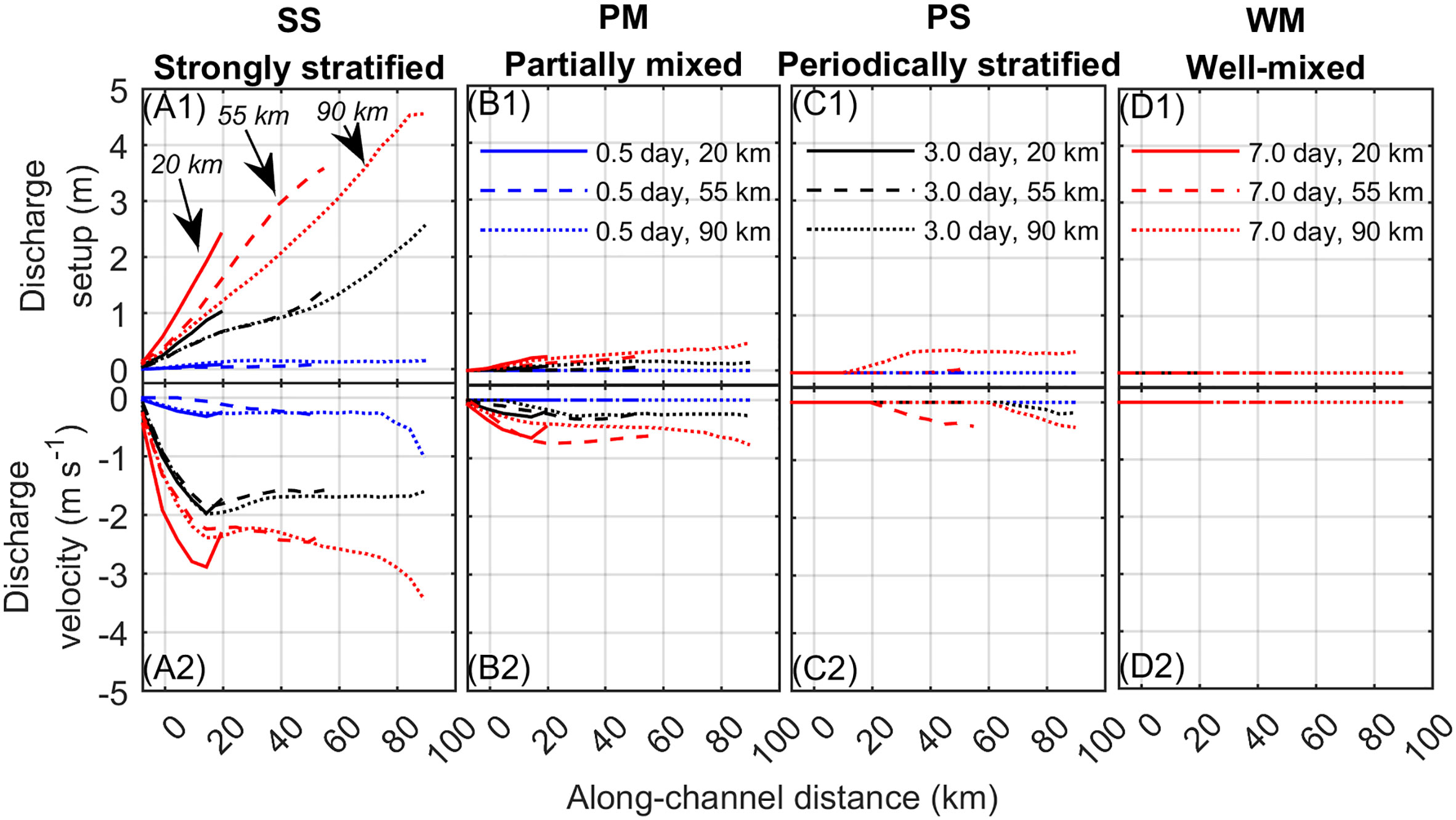
Figure 7 Along-channel profiles of (A1-D1) discharge setup (m) and (A2-D2) velocity (m s^-1) depending on estuarine type, dam location, and discharge interval. Along-channel distance is distance from the estuarine mouth (positive landward). Negative current is seaward.

A similar pattern was observed in the post-dam PM estuary. The discharge setup was less, reaching up to 0.5 m ($P{M}_{90}^7$), as was the magnitude of the discharge velocity, reached nearly 1 m s^-1 ($P{M}_{90}^7$). In the tide-dominated, post-dam PS estuary, a significant discharge pulse was generated only for the long discharge interval of Δt = 7 days. Also, the pulse dissipated completely before reaching the mouth. In the tide-dominated, post-dam WM estuary, the freshwater discharge was the least, and no significant pulse was observed. These results indicate that the river-dominated estuaries are particularly susceptible to discharge pulses, which are greater with increasing discharge interval, and are able to reach the mouth. For tide-dominated estuaries, only the longest discharge interval made a pulse, and it fully dissipated before reaching the mouth.

3.3 Effect of tide and river change on salinity, exchange flow, and estuarine classification

3.3.1 Salinity, stratification, and the estuarine exchange flow

This section considers changes in salt and baroclinic processes which result from the combined changes to the tide and river forcing. These processes are of interest to gain insight into the effect of the estuarine dam on salt and sediment transport. As data for different discharge intervals were similar, the effect of the dam location is primarily considered.

Along-channel profiles of salinity, stratification, and the estuarine exchange flow parameter for the discharge interval Δt = 3 days are shown in Figure 8. For the pre-dam estuaries the salt intrusion increased from the SS to WM estuary (Figures 8A1-D1). The stratification increased from the WM to SS estuary (Figures 8A2-D2) as did the exchange flow parameter (Figures 8A3-D3). The exchange flow was greater in the pre-dam SS compared to the PM estuary because of strong freshwater outflow in the surface layer of the SS estuary which is included in the exchange flow parameter, μ.

FIGURE 8

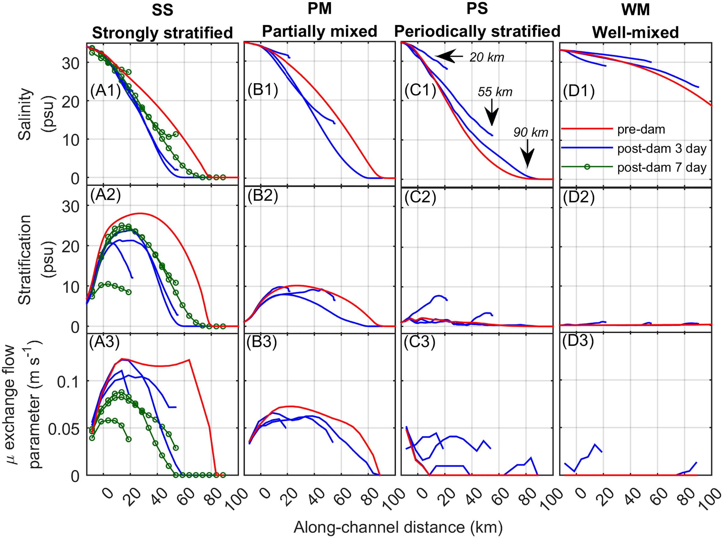
Figure 8 Along-channel profiles depending on estuarine type, dam location, and discharge interval of (A1-D1) depth-averaged salinity (psu), (A2-D2) top-to-bottom salinity stratification (psu), and (A3-D3) estuarine circulation parameter μ (m s^-1). Along-channel distance is distance from the estuarine mouth (positive landward). Most post-dam data is for discharge interval Δt = 3 days. The post-dam data for discharge interval Δt = 7 days is shown for the strongly stratified estuary.

The estuarine dam located at x = 90 km was near the salt intrusion limit for the SS, PM, and PS estuaries, whereas it was located with the salt intrusion for the WM estuary (Figures 8A1-D1). The post-dam river-dominated estuaries tended to get fresher, less stratified, and have decreased exchange flow (Figures 8A1-A3, B1-B3). This was mainly due to the shift from steady two-layer circulation to unsteady freshwater fronts. Greater discharge interval for $S{S}_x^7$ tended to show higher salinity and stratification and less exchange flow which was due to greater freshwater conveyance, intrusion of salt along the bottom layer during quiescent periods, and discharge unsteadiness. The post-dam tide-dominated estuaries tended to get saltier, more stratified, and have increased exchange flow (Figures 8C1-C3, D1-D3). This was due to the shift from a mixed water column to freshwater pulses conveyed to the shelf primarily along the surface and reduced mixing. The $P{M}_{20}^3$ and $W{M}_{20}^3$ estuaries were exceptions for their post-dam salinity change due to differences in stratification and the seaward conveyance of freshwater in the short x = 20 km estuaries.

Overall it was found that the response of the salinity, stratification, and exchange flow are influenced by changes in mixing caused by reduced tidal currents as well as the discharge pulse. Comparing the estuarine types, estuarine dams located further inland affected river-dominated estuaries more by making their inland portions fresh with less exchange flow (Figures 8A1-A3, B1-B3), and estuarine dams located further seaward affected tide-dominated estuaries more by making the mouths more stratified with greater exchange flow (Figures 8C1-C3, D1-D3). Higher discharge interval resulted in similar spatial trends (Figures 8A1-A3). It is likely the discharge interval interacted with a flushing time scale. Thus $S{S}_{90}^7$ was saltier than $S{S}_{90}^3$ because the discharge interval was greater than the flushing time scale. This relationship is complex as the flushing time scale is a function of the discharge interval (Azevedo et al., 2010) and reasonably the dam location because of its effect on the estuarine volume and tidal currents.

3.3.2 Estuarine parameter space

The change in estuarine classification is shown in Figure 9 with the divisions of the estuarine parameter space into different estuarine types labeled in Figure 9A3 for reference. For the pre-dam estuaries, lower and higher M represent primarily neap and spring tide variation, respectively, and lower and higher Fr_f represent seaward and landward position. The pre-dam estuaries matched their estuarine type (Figure 9, no dam).

FIGURE 9

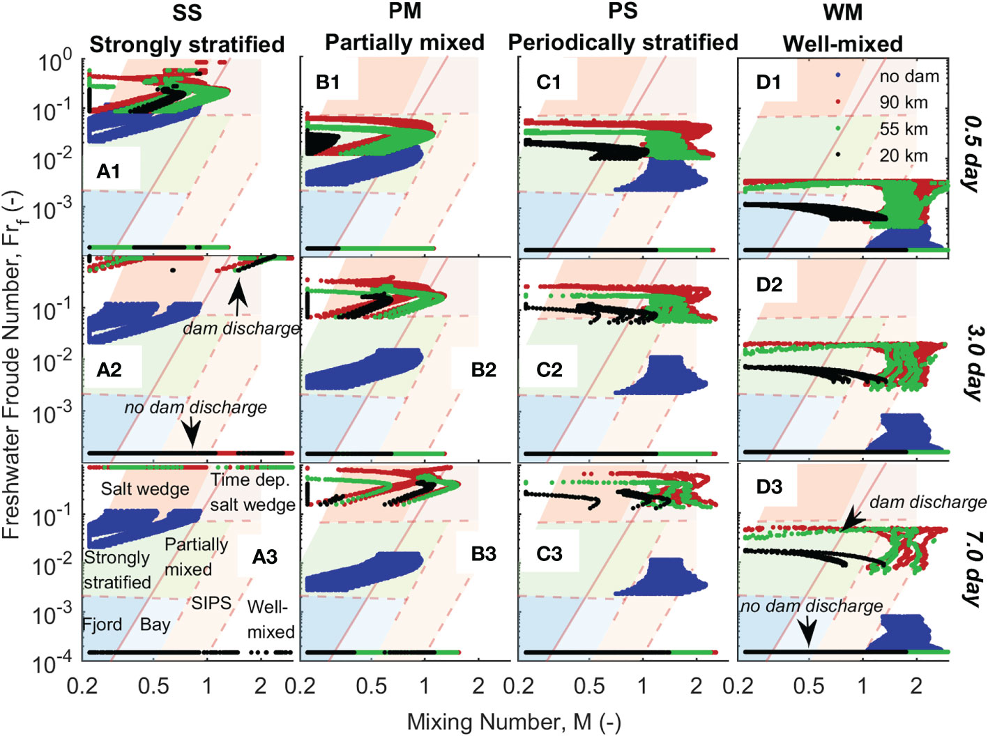
Figure 9 Change in estuarine classification for each estuary type depending on estuarine dam location and discharge interval: (A1-D1) Δt = 0.5 day, (A2-D2) Δt = 3 day, and (A3-D3) Δt = 7 day. Minimum values of M = 0.22 and Fr_f = 1.5 × 10^-4 and a maximum value of Fr_f = 0.9 were specified. Physically, these represent very low currents, very low freshwater discharge, and very high freshwater discharge approaching the maximum baroclinic frontal propagation speed, respectively. SIPS is strain-induced periodically stratified estuary, also referred to as a periodically stratified estuary.

Overall, the estuarine dam resulted in significant change in the estuarine type for all the post-dam estuaries due to changes in river and tidal forcing. A key change in the post-dam estuaries was high Fr_f during dam discharge and low Fr_f during no dam discharge (labeled for example in Figure 9A2, D3). During dam discharge, the estuaries tended to shift to the salt wedge and time dependent salt wedge types (Figures 9A1-A3, B2-B3, C2-C3, dam discharge), and during no dam discharge, the estuaries tended to shift to fjord, bay, SIPS, and well-mixed types (Figures 9A1-D3, no dam discharge). The Fr_f at unity or greater during dam discharge for the pre-dam SS estuary indicated that the maximum baroclinic frontal propagation speed was at times being replaced by a barotropic propagation speed as salt water was being pushed out of the estuary. Additionally, the post-dam Fr_f increased more for longer discharge periods (Δt = 7 days, Figures 9A3-D3) compared to shorter discharge periods (Δt = 0.5 days, Figures 9A1-D1).

The mixing number M changed in two ways. First, M was reduced in all cases in the area adjacent to the estuarine dam and in the case of dam location x = 20 km (see, e.g., Figure 9D3). The area adjacent to the dam shows M reducing quickly because of the dead-end channel. The dam location of x = 20 km had the most reduced M because of the dead-end channel and loss of tidal prism. This occurred in all post-dam estuaries but was most noticeable in the tide-dominated estuaries (Figures 9C1-C3, D1-D3, 20 km). Second, M increased adjacent to the estuarine dam during discharges due to the strong discharge currents. This was most apparent in the river-dominated estuaries (see, e.g. Figures 9A1-A3, B1-B3, dam discharge).

Considering the change in Fr_f and M together, it was revealed that the greatest change in estuarine type occurred for dams near the mouth with long discharge intervals (x = 20 km and Δt = 7 days). Furthermore, the post-dam river-dominated estuaries varied more than the tide-dominated estuaries due to the greater range in Fr_f, where $S{S}_x^7$ was an extreme case alternating between, for example, time dependent salt wedge and bay (Figure 9A3).

3.4 Effect of tide and river change on sediment flux decomposition and morphology

3.4.1 Along-channel depth, mud fraction, fluvial fraction, SSC, and sediment flux

Changes in tide and river due to an estuarine dam can affect the currents, sediment sources, and so forth. Change in aspects of sediment and morphodynamics according to an estuarine dam is shown in Figure 10. As the discharge interval resulted in similar trends, the effect of dam location for cases with Δt = 3 days is primarily considered. The effect of the discharge interval on bathymetry and cross-sectionally integrated sediment flux is shown for the post-dam SS estuary (Figures 10A1, A5).

FIGURE 10

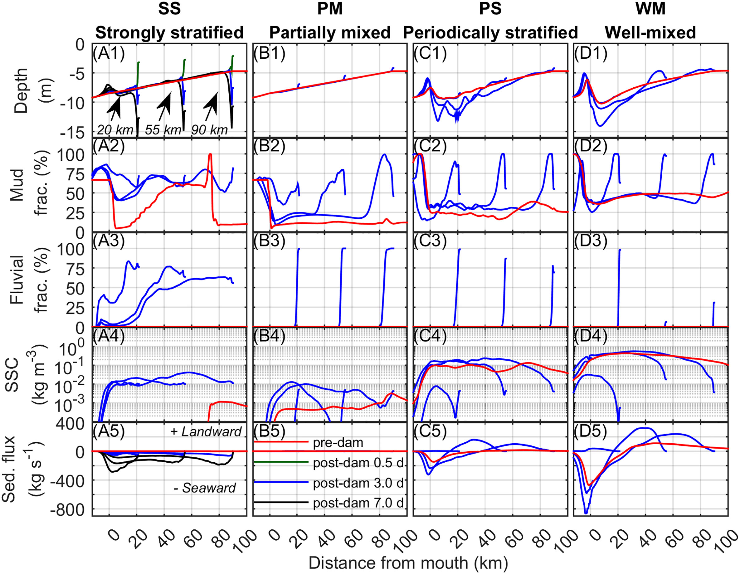
Figure 10 Pre-dam and post-dam along-channel profiles depending on estuarine dam location (dam at x = 20, 55, and 90 km) of (A1-D1) width-averaged channel depth (m), (A2-D2) width-averaged mud fraction (%) on bed surface, (A3-D3) width-averaged fluvial sediment fraction (%) on bed surface, (A4-D4) depth-averaged suspended sediment concentration along channel thalweg (SSC, kg m^-3), and (A5-D5) cross-sectionally integrated sediment flux (kg s^-1). Most data correspond to Δt = 3 day. In (A1, A5) Δt = 0.5 and 7 day are also shown. Along-channel distance is distance from the estuarine mouth (positive landward). Negative current is seaward.

The pre-dam conditions can be summarized as follows. The river-dominated estuaries’ depths tended to have less change from the initial condition whereas the tide-dominated estuaries tended to have more because of the Stokes return flow causing a deepening of the mouth and formation of a mouth bar (Figures 10A1-D1). Along the channel the bed was primarily sandy and the shelf was muddy (Figures 10A2-D2). In all cases there was no fluvial sediment reaching the estuary (Figures 10A3-D3). The SSC increased from the river-dominated estuaries to the tide-dominated estuaries (Figures 10A4-D4). And, the magnitude of the sediment flux was increasing from relatively negligible in the river-dominated estuaries to the strongest in the tide-dominated estuaries where the sediment flux was mostly seaward at the mouth due to the Stokes return flow (Figures 10A5-D5).

Similar to the pre-dam estuaries, the post-dam estuaries could be divided into two groups based on their dynamics, the river-dominated and the tide-dominated estuaries, with the PM estuary being transitional between the two. The $S{S}_x^{0.5}$ and $P{M}_x^3$ showed the formation of bayhead delta deposits due to input of fluvial sediments directly into estuary from the dam, however for longer discharge intervals, the SS estuary showed the formation of scour near the dam and deposits further downstream (Figures 10A1-A2). The tide-dominated estuaries with x = 20 km showed relatively little post-dam morphodynamic change, whereas x = 55 and 90 km showed deepening and bar formation at the mouth but also notably deposition adjacent to the dam due to tidal asymmetry. The estuaries became muddier due to discharge of fluvial mud in the river-dominated estuaries and the deposition of mud from suspension in the tide-dominated estuaries (Figures 10A2-D2). The amount of the fluvial sediment increased in all estuaries near the dam, and throughout the estuaries for the high freshwater discharge post-dam SS estuary (Figures 10A3-D3). The SSC tended to increase for the river-dominated estuaries due to input of sediment and resuspension by discharge pulses, and it tended to decease for the tide-dominated estuaries due to reduction of the tidal currents, particularly for x = 20 km (Figures 10A4-D4). Finally, the relatively small sediment fluxes increased considerably to seaward fluxes in the post-dam SS estuary, the fluxes remained low in the post-dam PM estuary, and the post-dam tide-dominated estuaries showed a similar pattern as their pre-dam estuaries, yet there was a notable increase in the landward sediment fluxes due to changes in the Stokes return flow and tidal asymmetry (Figures 10A5-D5). Based on these results, it can be seen that the dam location affected the response of the tide-dominated estuaries, and the discharge interval affected the river-dominated estuaries, in particular whether deposition or scour occurred adjacent to the dam. The changes in fluvial sediment and sediment flux directions also indicate that the river-dominated estuaries are primarily receiving sediment from the river boundary whereas the tide-dominated estuaries are primarily receiving sediment from the marine sediments reworked from the estuary and shelf.

3.4.2 Sediment flux decomposition

The decomposed sediment fluxes are shown in Figure 11. As different discharge intervals resulted in similar trends, the effect of dam location for cases with Δt = 3 days is considered. Overall, the sediment flux mechanisms and their response to the estuarine dam could be divided into the river- and tide-dominated estuaries with the PM estuary being transitional between the two.

FIGURE 11

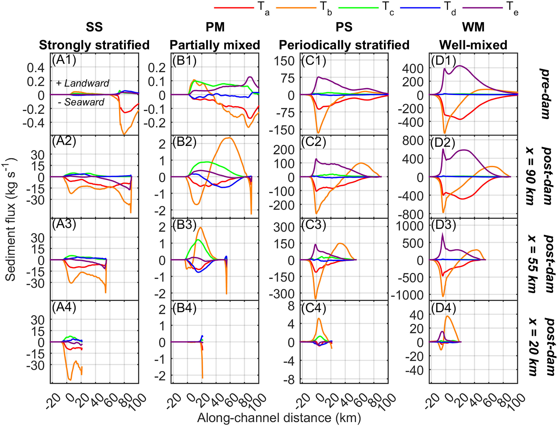
Figure 11 Pre- and post-dam spring-neap averaged, cross-sectionally integrated decomposed sediment flux (kg s^-1) along-channel profiles depending on estuarine type and estuarine dam location for (A1-D1) the pre-dam estuaries, (A2-D2) dam at x = 90 km, (A3-D3) dam at x = 55 km, and (A4-D4) dam at x = 20 km for discharge interval Δt = 3 days. T_a is the transport by averages due river runoff or Stokes return flow, T_b is tidal pumping, T_c is estuarine exchange flow, T_d is tidal straining, and T_e is Stokes transport. Along-channel distance is distance from the estuarine mouth, positive is landward. Positive sediment flux is landward.

For the pre-dam SS estuary, seaward river runoff (T_a) and tidal pumping (T_b) by Euler-induced tidal asymmetry were the main mechanisms in the landward tidal river portion, and this led to the two-layered estuary with relatively small sediment fluxes on the seaward side (Figure 11A1). With the estuarine dam, the magnitude of the fluxes increased and T_a and T_b extended throughout the estuary until reaching the shelf (Figures 11A2-A4). As the dam approached the mouth, the importance of seaward tidal pumping increased as did some landward estuarine exchange flow (T_c). In this case, the seaward T_b was due to the intratidal discharge pulses instead of the Euler-induced tidal asymmetry which occurred in the tidal river of the pre-dam estuary due to tides interacting with the seaward river runoff.

For the pre-dam PM estuary, the tidal straining (T_d) and Stokes transport (T_e) also made contributions to the sediment flux (Figure 11B1), yet it is noted that T_d was generally found to be negligible in this study. In the pre-dam PM estuary, landward T_c and related T_b due to Euler-induced tidal asymmetry occurred near the mouth whereas toward the head seaward T_a and T_b occurred, similar to the pre-dam SS estuary. Some landward T_e was present as the tides were of moderate range and mixed. With the estuarine dam at x = 55 and 90 km, two areas could be distinguished (Figures 11B2-B3). First, adjacent to the estuarine dam is a narrow area where the intratidal discharge causes a seaward T_b. Second is the broader area of the estuary where T_a and T_b flush some sediment seaward and primarily T_c and associated T_b due to Euler-induced asymmetry bring sediment landward. With x = 20 km, freshwater is conveyed efficiently to the shelf. T_c is reduced, and T_b in the narrow area adjacent to the dam is only active due to discharge pulses while the rest of the estuary is quiescent due to the reduced tidal currents.

The pre-dam tide-dominated estuaries (PS and WM) were both found to be strongly affected by the Stokes drift (T_e), Stokes return flow (here T_a), and tidal pumping (T_b) due to the Euler-induced tidal asymmetry caused by the interaction of the Stokes return flow Eulerian residual current and the strong tidal currents (Figures 11C1-D1). As discussed in Figueroa et al. (2022), in tide-dominated estuaries with little freshwater input, T_a is better to be thought of as a mean flux due to the Stokes return flow rather than a mean flux due to the river runoff. It is for this reason there is a symmetry between landward T_e and seaward T_a in Figures 11C1-D1. While T_a and T_e approximately balance, the Stokes return flow Eulerian residual current generates the seaward T_b due to the Euler-induced tidal asymmetry. With the estuarine dam at x = 55 and 90 km, the tides become standing near the estuarine dam, resulting in the elimination of Stokes drift there and promotion landward T_b due to landward tidal distortion and interaction of the M₂ and M₄ constituents. Landward T_b was likely also promoted by the reduction of the Stokes setup and amplification of the tides which would tend to deform the tides more and promote flood-dominance. With x = 20 km, the tides were standing and the Stokes drift was effectively eliminated (Figures 11C4-D4). Thus, the landward T_b due to tidal deformation dominated with some landward T_c in the ${\text{PS}}_{20}^3$ estuary and some landward T_e over the mouth bar in the ${\text{WM}}_{20}^3$ estuary (Figures 11C4, D4, respectively).

These results indicate that as the estuarine dam location approached the mouth there was a continuous change in the sediment flux mechanisms, including their magnitudes and directions. The river-dominated SS estuary shifted to higher magnitude sediment fluxes which were seaward due to the discharge pulse and could scour sediments. The PM estuary experienced changes in T_c and T_b, and when the estuary become very short, the tides were significantly reduced resulting in a shift to a quiescent basin receiving the discharged fluvial sediments. Finally, the tide-dominated estuaries were characterized by the reduction of the Stokes drift due the shift from a mixed to a standing tidal wave. This occurred first adjacent to the estuarine dam, but then came to cover the entire estuary when the estuary became very short. For these parts, T_b was reduced in magnitude but changed direction to landward indicating reworking of the mouth bar and import of marine sediments from the shelf due to tidal distortion and interaction of the M₂ and M₄ constituents.

4 Discussion

4.1 Interaction of dam location and discharge interval with estuarine spatial and temporal scales

The overall objective of this study is to understand the effect of estuarine dam location and discharge interval on estuarine processes. It was revealed that the estuarine dam location and discharge interval are important parameters controlling tide and river processes, respectively, and that the estuarine response depends on the estuarine type, broadly river-dominated and tide-dominated estuaries.

In the tide-dominated estuaries, the estuarine dam location was important due to the processes of wave reflection, resonance, the dead-end channel, loss of tidal prism, and shift from progressive and mixed to standing tidal waves. The resonance length was found to be an important length scale determining the estuarine response, and its value (here approximately L/8 = 45 km) was noted as being less than the classical value (L/4 = 90 km) due to friction. For dams located a distance less than the resonance length from the mouth, the switch from mixed to standing tides reduced the Stokes drift, Stokes setup, Stokes return flow Eulerian residual current, and the seaward tidal pumping due to Euler-induced tidal asymmetry. This resulted in lower mean sea levels, reduced seaward Eulerian residual current, and establishment of landward tidal pumping due to tidal deformation likely supported by the shallower water with amplified tides. For dams located near the resonance length, the mouth was deepened due to the increased currents which resulted in a morphodynamic feedback bringing the currents back to a magnitude similar to the pre-dam condition. The reworking of sediment at the mouth together with the dead-end channel and standing tides near the dam resulted in the greatest deposition near the estuarine dam. For dams located further than the resonance length, the pattern of seaward tidal pumping at the mouth where the tides were mixed resembled the pre-dam estuary, but landward tidal pumping near estuarine dam was prevalent due to the standing tides and flood-dominance due to shallow water tidal deformation.

In addition to the resonance length, the tidal excursion (typically about 14 km; Savenije, 2005) may also be a relevant length scale. This is because in tide-dominated estuaries receiving relatively low discharge, the seaward discharge pulse velocity is not much greater than the ebb current. Thus, the freshwater can travel approximately a tidal excursion before the turn of the tide. Therefore, if the estuarine dam location from the mouth is further than the tidal excursion, more than one tidal cycle is needed for the freshwater to reach the mouth, which can result in discharged fluvial sediments settling and being trapped in the estuary and an inability of the freshwater discharge to resuspend and flush sediments seaward (Figueroa et al., 2020b).

In the river-dominated estuaries, the discharge interval was important due to the processes of discharge water level setup, discharge pulse, exchange flow, freshwater fronts, sediment resuspension, and scour. The tidal cycle period (T = 12.4 hr ≈ 0.5 days) was found to be an important time scale determining the estuarine response to discharge. For a discharge interval equal to the tidal cycle period (Δt = 0.5 days, i.e. once every ebb tide), the sea surface elevations, currents, stratification, and sediment resuspension and settling cycles in the post-dam SS estuary resembled the pre-dam conditions. For discharge intervals longer than the tidal time scale (Δt = 3 and 7 days), the discharge currents were much greater than the pre-dam condition and the SS estuary shifted from being a continuously two-layered system to being a time-varying layered system strongly modified by discharge pulses, freshwater fronts, and discharge resuspension. There was also a switch from the deposition of a bayhead delta composed of fluvial sediment adjacent to the estuarine dam to the formation of a scour hole. It can be noted that as the discharge interval scaled with the discharge volume in this study, greater discharge intervals also imply greater ratios of discharge volume to estuarine volume during a discharge event which reasonably is important in determining the pattern of estuarine response, with larger values tending away from the pre-dam behavior.

In addition to the tidal time scale, the flushing time scale is also relevant for the transport of freshwater. For discharge intervals less than the flushing time scale, freshwater may accumulate in the estuary, whereas for discharge intervals greater than the flushing time scale, the estuary will be saltier. However, defining the flushing time scale is challenging due to its dependence on the discharge interval, dam location, and internal processes.

4.2 Implications for coastal hazards

Estuarine dams can provide several societal benefits such as increased freshwater supply for agriculture, stabilized upstream water levels, improved upstream navigability, and often a causeway constructed along the estuarine dam which improves the transportation infrastructure. At the same time, these benefits can be a trade-off with increased risks to coastal hazards such as coastal flooding, coastal erosion, harbor siltation, and water quality issues including eutrophication, algal blooms, and hypoxia. These trade-offs are not limited to the estuary but also include the upstream river and downstream shelf which are also affected by the change in tide and river processes and interruption of the sediment transport pathway.

Estuarine dams can affect coastal flooding in two ways. First, this study indicates that discharge setup and amplification of the tides can be greater than the reduction of the mean sea level by diminished Stokes setup. An example of where this has occurred is the Bang Pakong estuary, Thailand, where unexpected tidal amplification resulted in bank erosion and coastal flooding of saline water (Vongvisessomjai and Srivihok, 2003). Second, this study indicated that for most scenarios fluvial and marine sediments were deposited adjacent to the sluice gates. This can increase the risk of flooding due to the reduced drainage capacity of the river (Zhu et al., 2017; Tilai et al., 2019).

Estuarine dams also have implications for harbor siltation and water quality. For the post-dam tide-dominated estuaries, flood-dominated tidal pumping brought marine sediments reworked from the estuarine mouth or shelf and deposited them in the area with minimum currents. For the post-dam river dominated estuaries, fluvial sediments were deposited as a bay head delta and also scoured sediment were transported seaward, in some cases depositing as a mouth bar. These patterns suggest that the post-dam estuaries are susceptible to siltation and shoaling of the mouth which will require dredging to maintain navigability for any harbor developments. With respect to water quality, most scenarios in this study showed reduced SSC due to reduced currents. Together with nutrient inputs from the watershed, increased water clarity can result in algal blooms (Jeong et al., 2014) which may impact the benthic habitats and fisheries.

Investigation of alternative dam locations and discharge intervals in this study suggests that the estuarine dam always significantly impacts the estuary. Dams located further upstream beyond the resonance length with discharge intervals on the order of the tidal cycle period were found to most resemble the pre-dam estuaries in terms of tidal dynamics, discharge velocity, SSC, sediment fluxes, and depth. However, this dam location and operation, while minimizing the dam impact, limits the ability of the estuarine dam to block the salt intrusion and store freshwater which is in many cases their primary purpose. Nevertheless, while simplified idealized modeling provides a useful tool for understanding patterns in the estuarine response, in practice optimization of the dam location and discharge interval to reduce impacts to a specific estuary will depend the details of the estuary such as the more realistic geometry, forcing, and sediment sources.

4.3 Reliability of idealized estuary model

The idealized model appears to aid in understanding first-order impacts of estuarine dams with sluices gates for a range of estuarine types, dam locations, and discharge intervals. However, it should be noted that the estuarine geometry (mouth depth, mouth width, bottom slope, width convergence), estuarine forcing (semidiurnal tides, no waves, no seasonal or interannual discharge variation), and sedimentary aspects (non-cohesive sediment and short morphological time scales) shape the result.

As this study focused primarily on the along-channel dynamics, future research can increase our understanding by evaluating trends in the across-channel, vertical, and temporal dynamics. Furthermore, more research is needed to understand the reservoir. In this study, it is assumed that the inflow is constant and the reservoir is large, so the discharge interval is determined a priori by a dam operator. But in general, the upper bound for possible discharge interval is determined by the reservoir volume and freshwater inflow rate. In addition to its effect on the discharge interval, the reservoir is also coupled to the post-dam estuary by influencing the water quality entering the post-dam estuary (Jeong et al., 2014). Over long time scales, the reservoir can fill with sediments and particulate nutrients and then become a source for the downstream estuary (Palinkas et al., 2019). This research would help to better link the reservoir and post-dam estuary sub-environments.

Together with the reservoir, more research can be done on the different gate types. This appears to be important for estuarine dams which are located further upstream or function primarily as hydroelectric plants, weirs and locks. Examples include the Saco Dam on the Saco estuary, Maine (Kelley et al., 2005), the Federal Dam on the Hudson estuary, New York (Ralston et al., 2019), the Conowingo Dam on the Susquehanna estuary, Maryland (Palinkas et al., 2019), and the Franklin Lock and Dam on the Caloosahatchee estuary, Florida (Buzzelli et al., 2014) in the US. These examples fit the definition of an estuarine dam or weir here as they limit the upstream propagation of salt or tides. However, their structure and operation can be different from those applied in this study, with sluice gates discharging during ebb tide, which are found for example in Europe and Asia. This research on different structures and operation should help to bridge the gap between the effects of estuarine and river dams and weirs on estuaries.

5 Conclusions

This study has extended the results of Figueroa et al. (2022) for the effect of an estuarine dam on SS, PM, PS, and WM estuaries to a range of dam locations and discharge intervals. It was confirmed that changes in these parameters resulted in systematic changes in the river and tidal processes which in turn resulted in changes in the estuarine classification, sediment dynamics, and morphodynamics. Some key findings of this research are:

● The dam location primarily impacted the tide-dominated estuaries, and the resonance length was an important length scale. When the dam was seaward of the resonance length, the tidal currents were strongly reduced due to tidal prism loss and the dead-end channel. When the dam was at the resonance length, the morphology adjusted and maintained tidal currents near the mouth, but tidal currents were reduced near the dam due to the dead-end channel. When the dam was landward of the resonance length, the tidal currents were mostly reduced near the dam due to the dead-end channel.

● The discharge interval primarily impacted the river-dominated estuaries, and the tidal cycle was an important time scale. When the discharge interval was less than the tidal cycle period, the estuaries maintained similar salinity and stratification. When the discharge interval was greater than the tidal cycle period, the estuaries began to experience notable seaward discharge pulses and discharge freshwater fronts.

● Dams located near the mouth with large discharge intervals, associated with large discharge magnitudes, differed the most from their pre-dam condition in the estuarine parameter space. Conversely, dams located near the estuary head with small discharge intervals, associated with small discharge magnitudes, differed the least from their pre-dam condition in the estuarine parameter space.

● Dams located near the mouth altered the sediment flux mechanisms the most for all estuaries. The river-dominated estuaries were characterized by a shift from landward flux due to estuarine exchange flow to seaward flux due to river runoff and tidal pumping by the intratidal discharge pulses. The tide-dominated estuaries were characterized by a shift from seaward flux due to Stokes return flow and tidal pumping due to Euler-induced tidal asymmetry to landward flux due to tidal pumping by tidal distortion and M₂-M₄ interaction in the shallow, macrotidal estuaries.

It is expected this research will be valuable as estuarine dams continue to be constructed (e.g., the Bhadbhut barrage on the Narmada River, India; The Times of India, 2021) and are likely to become more prevalent in the future as sea level rise increases the salt and tidal intrusions, in addition to potentially less river runoff in some areas and dredging to accommodate larger ships (Winterwerp and Wang, 2013; Nienhuis et al., 2018; Nienhuis and van de Wal, 2021).

Data availability statement

The raw data supporting the conclusions of this article will be made available by the authors, without undue reservation.

Author contributions

SF, conceptualization, data curation, formal analysis, funding acquisition, investigation, methodology, validation, and visualization. MS, data curation, funding acquisition, investigation, project administration, supervision, and validation. GL, conceptualization, data curation, investigation, methodology, and validation.

Funding

This research was supported by research fund of Chungnam National University.

Conflict of interest

The authors declare that the research was conducted in the absence of any commercial or financial relationships that could be construed as a potential conflict of interest.

Publisher’s note

All claims expressed in this article are solely those of the authors and do not necessarily represent those of their affiliated organizations, or those of the publisher, the editors and the reviewers. Any product that may be evaluated in this article, or claim that may be made by its manufacturer, is not guaranteed or endorsed by the publisher.

Supplementary material

The Supplementary Material for this article can be found online at: https://www.frontiersin.org/articles/10.3389/fmars.2022.1035501/full#supplementarymaterial

References

Azevedo I. C., Bordalo A. A., Duarte P. M. (2010). Influence of river discharge patterns on the hydrodynamics and potential contaminant dispersion in the douro estuary (Portugal). Water Res. 44 (10), 3133–3146. doi: 10.1016/j.watres.2010.03.011

PubMed Abstract | CrossRef Full Text | Google Scholar

Burchard H., Hetland R. D. (2010). Quantifying the contributions of tidal straining and gravitational circulation to residual circulation in periodically stratified tidal estuaries. J. Phys. Oceanography 40 (6), 1243–1262. doi: 10.1175/2010JPO4270.1

CrossRef Full Text | Google Scholar

Burchard H., Schuttelaars H. M., Ralston D. K. (2018). Sediment trapping in estuaries. Annu. Rev. Mar. Sci. 10, 371–395. doi: 10.1146/annurev-marine-010816-060535

CrossRef Full Text | Google Scholar

Buzzelli C., Doering P. H., Wan Y., Sun D., Fugate D. (2014). Modeling ecosystem processes with variable freshwater inflow to the caloosahatchee river estuary, southwest florida. i. model development. Estuarine Coast. Shelf Sci. 151, 256–271. doi: 10.1016/j.ecss.2014.08.028

CrossRef Full Text | Google Scholar

Cai H., Toffolon M., Savenije H. H. (2016). An analytical approach to determining resonance in semi-closed convergent tidal channels. Coast. Eng. J. 58 (03), 1650009. doi: 10.1142/S0578563416500091

CrossRef Full Text | Google Scholar

Díez-Minguito M., Baquerizo A., Ortega-Sánchez M., Navarro G., Losada M. A. (2012). Tide transformation in the guadalquivir estuary (SW Spain) and process-based zonation. J. Geophysical Res.: Oceans 117 (C3), C03019. doi: 10.1029/2011JC007344

CrossRef Full Text | Google Scholar

Figueroa S. M., Lee G., Chang J., Jung N. W. (2022). Impact of estuarine dams on the estuarine parameter space and sediment flux decomposition idealized numerical modeling study. J. Geophysical Res.: Oceans, 127 (5), e2021JC017829. doi: 10.1029/2021JC017829

CrossRef Full Text | Google Scholar

Figueroa S. M., Lee G., Chang J., Schieder N. W., Kim K., Kim S. Y. (2020b). Evaluation of along-channel sediment flux gradients in an anthropocene estuary with an estuarine dam. Mar. Geol. 429, 106318. doi: 10.1016/j.margeo.2020.106318

CrossRef Full Text | Google Scholar

Figueroa S. M., Lee G., Shin H. J. (2019). The effect of periodic stratification on floc size distribution and its tidal and vertical variability: Geum estuary, south Korea. Mar. Geol. 412, 187–198. doi: 10.1016/j.margeo.2019.03.009

CrossRef Full Text | Google Scholar

Figueroa S. M., Lee G., Shin H. J. (2020a). Effects of an estuarine dam on sediment flux mechanisms in a shallow, macrotidal estuary. Estuarine Coast. Shelf Sci. 238, 106718. doi: 10.1016/j.ecss.2020.106718

CrossRef Full Text | Google Scholar

Friedrichs C. T. (2010). Barotropic tides in channelized estuaries. Contemp. Issues Estuar. Physics 27, 61. doi: 10.1017/CBO9780511676567.004

CrossRef Full Text | Google Scholar

Friedrichs C. T., Aubrey D. G. (1988). Non-linear tidal distortion in shallow well-mixed estuaries: a synthesis. Estuarine Coast. Shelf Sci. 27 (5), 521–545. doi: 10.1016/0272-7714(88)90082-0

CrossRef Full Text | Google Scholar

Geyer W. R., MacCready P. (2014). The estuarine circulation. Annu. Rev. Fluid Mechanics 46 (1), 175–197. doi: 10.1146/annurev-fluid-010313-141302

CrossRef Full Text | Google Scholar

Guo L., Wang Z. B., Townend I., He Q. (2019). Quantification of tidal asymmetry and its nonstationary variations. J. Geophysical Res.: Oceans 124 (1), 773–787. doi: 10.1029/2018JC014372

CrossRef Full Text | Google Scholar

Guo L., Van der Wegen M., Roelvink J. A., He Q. (2014). The role of river flow and tidal asymmetry on 1-D estuarine morphodynamics. Journal of Geophysical Research: Earth's Surface 119(11), 2315–34. doi: 10.1002/2014JF003110

CrossRef Full Text | Google Scholar

Haddout S., Maslouhi A. (2019). Testing analytical tidal propagation models of the one-dimensional hydrodynamic equations in morocco's estuaries. Int. J. River Basin Management 17 (3), 353–366. doi: 10.1080/15715124.2018.1546721

CrossRef Full Text | Google Scholar

Haidvogel D. B., Arango H., Budgell W. P., Cornuelle B. D., Curchitser E., Di Lorenzo E., et al. (2008). Ocean forecasting in terrain-following coordinates: Formulation and skill assessment of the regional ocean modeling system. J. Comput. Physics 227 (7), 3595–3624. doi: 10.1016/j.jcp.2007.06.016

CrossRef Full Text | Google Scholar

Hoitink A. J. F., Jay D. A. (2016). Tidal river dynamics: Implications for deltas. Rev. Geophysics 54 (1), 240–272. doi: 10.1002/2015RG000507

CrossRef Full Text | Google Scholar

Jay D. A., Leffler K., Diefenderfer H. L., Borde A. B. (2015). Tidal-fluvial and estuarine processes in the lower Columbia river: I. along-channel water level variations, pacific ocean to Bonneville dam. Estuaries Coasts 38 (2), 415–433. doi: 10.1007/s12237-014-9819-0

CrossRef Full Text | Google Scholar

Jeong Y. H., Yang J. S., Park K. (2014). Changes in water quality after the construction of an estuary dam in the geum river estuary dam system, Korea. J. Coast. Res. 30 (6), 1278–1286. doi: 10.2112/JCOASTRES-D-13-00081.1

CrossRef Full Text | Google Scholar

Kelley J. T., Barber D. C., Belknap D. F., FitzGerald D. M., van Heteren S., Stephen M., et al. (2005). Sand budgets at geological, historical and contemporary time scales for a developed beach system, saco bay, Maine, USA. Mar. Geol. 214 (1–3), 117–142. doi: 10.1016/j.margeo.2004.10.027

CrossRef Full Text | Google Scholar

Kukulka T., Jay D. A. (2003). Impacts of Columbia river discharge on salmonid habitat: 1. a nonstationary fluvial tide model. J. Geophysical Res.: Oceans 108 (C9), 3293. doi: 10.1029/2002JC001382

CrossRef Full Text | Google Scholar

Laffaille P., Caraguel J. M., Legault A. (2007). Temporal patterns in the upstream migration of European glass eels (Anguilla anguilla) at the couesnon estuarine dam. Estuarine Coast. Shelf Sci. 73 (1-2), 81–90. doi: 10.1016/j.ecss.2006.12.011

CrossRef Full Text | Google Scholar

Li M., Ge J., Kappenberg J., Much D., Nino O., Chen Z. (2014). Morphodynamic processes of the Elbe river estuary, Germany: the Coriolis effect, tidal asymmetry and human dredging. Front. Earth Sci. 8 (2), 181–189. doi: 10.1007/s11707-013-0418-3

CrossRef Full Text | Google Scholar

Milliman J. D., Farnsworth K. L. (2013). River discharge to the coastal ocean: A global synthesis (Cambridge, Cambridge University Press). doi: 10.1017/CBO9780511781247

CrossRef Full Text | Google Scholar

Moftakhari H. R., Jay D. A., Talke S. A. (2016). Estimating river discharge using multiple-tide gauges distributed along a channel. Journal of Geophysical Research: Oceans 121(4), 2078–97. doi: 10.1002/2015JC010983

CrossRef Full Text | Google Scholar

Nauw J. (2014). “Setup of a 3D hydrodynamic model of the Dutch western wadden Sea,” in NOIZ report. Den Burg: Royal Netherlands Institute for Sea Research (NOIZ)

Google Scholar

Nidzieko N. J. (2010). Tidal asymmetry in estuaries with mixed semidiurnal/diurnal tides. J. Geophysical Res.: Oceans 115 (C8), C08006. doi: 10.1029/2009JC005864

CrossRef Full Text | Google Scholar

Nidzieko N. J., Ralston D. K. (2012). Tidal asymmetry and velocity skew over tidal flats and shallow channels within a macrotidal river delta. J. Geophysical Res.: Oceans 117 (C3), C03001. doi: 10.1029/2011JC007384

CrossRef Full Text | Google Scholar

Nienhuis J. H., Hoitink A. J. F., Törnqvist T. E. (2018). Future change to tide-influenced deltas. Geophysical Res. Lett. 45 (8), 3499–3507. doi: 10.1029/2018GL077638

CrossRef Full Text | Google Scholar

Nienhuis J. H., van de Wal R. S. (2021). Projections of global delta land loss from sea-level rise in the 21st century. Geophysical Res. Lett. 48 (14), e2021GL093368. doi: 10.1029/2021GL093368

CrossRef Full Text | Google Scholar

Palinkas C. M., Testa J. M., Cornwell J. C., Li M., Sanford L. P. (2019). Influences of a river dam on delivery and fate of sediments and particulate nutrients to the adjacent estuary: Case study of conowingo dam and Chesapeake bay. Estuaries Coasts 42 (8), 2072–2095. doi: 10.1007/s12237-019-00634-x

CrossRef Full Text | Google Scholar

Pawlowicz R., Beardsley B., Lentz S. (2002). Classical tidal harmonic analysis including error estimates in MATLAB using T_TIDE. Comput. Geosci. 28 (8), 929–937. doi: 10.1016/S0098-3004(02)00013-4

CrossRef Full Text | Google Scholar

Ralston D. K., Talke S., Geyer W. R., Al-Zubaidi H. A., Sommerfield C. K. (2019). Bigger tides, less flooding: Effects of dredging on barotropic dynamics in a highly modified estuary. J. Geophysical Res.: Oceans 124 (1), 96–211. doi: 10.1029/2018JC014313

CrossRef Full Text | Google Scholar

Savenije H. H. (2005). Salinity and tides in alluvial estuaries (New York: Elsevier). doi: 10.1016/B978-0-444-52107-1.X5000-X

CrossRef Full Text | Google Scholar

Schuttelaars H. M., de Jonge V. N., Chernetsky A. (2013). Improving the predictive power when modelling physical effects of human interventions in estuarine systems. Ocean Coast. Management 79, 70–82. doi: 10.1016/j.ocecoaman.2012.05.009

CrossRef Full Text | Google Scholar

Shin H. J., Lee G., Kang K., Park K. (2019). Shift of estuarine type in altered estuaries. Anthropocene Coasts 2 (1), 145–170. doi: 10.1139/anc-2018-0013

CrossRef Full Text | Google Scholar

Shivaprasad A., Vinita J., Revichandran C., Manoj N. T., Srinivas K., Reny P. D., et al. (2013). Influence of saltwater barrage on tides, salinity, and chlorophyll a in Cochin estuary, India. J. Coast. Res. 29 (6), 1382–1390. doi: 10.2112/JCOASTRES-D-12-00067.1

CrossRef Full Text | Google Scholar

Syvitski J. P., Vorosmarty C. J., Kettner A. J., Green P. (2005). Impact of humans on the flux of terrestrial sediment to the global coastal ocean. Science 308 (5720), 376–380. doi: 10.1126/science.1109454

PubMed Abstract | CrossRef Full Text | Google Scholar

Syvitski J. P., Kettner A. (2011). Sediment flux and the Anthropocene. Jphilosophical transactions of the royal society a: Mathematical, physical and engineering sciences 369(1938), 957–975. doi: 10.1098/rsta.2010.0329

CrossRef Full Text | Google Scholar

Tabata K., Fukuoka S. (2014). “New computation method for flood flows and bed variations in a low-lying river with complex river systems,” in River Flow. Eds. Schleiss A. J., Cesare De J., Franca M. J., Pfister M. (London: Taylor & Francis Group), 1791–98.

Google Scholar

The Times of India (2021) Bhadbhut barrage to be ready by 2025. Available at: https://timesofindia.indiatimes.com/city/surat/bhadbhut-barrage-to-be-ready-by-2025/articleshow/85699621.cms (Accessed 25 August 2022).

Google Scholar

Tilai L., Liming C., Xiangyu G., Lei D. (2019). “Analysis of sediment deposition downstream tidal sluice of estuary,” in International conference on Asian and pacific coasts (Singapore: Springer), 649–655. doi: 10.1007/978-981-15-0291-0_89

CrossRef Full Text | Google Scholar

Traini C., Proust J. N., Menier D., Mathew M. J. (2015). Distinguishing natural evolution and human impact on estuarine morpho-sedimentary development: A case study from the vilaine estuary, France. Estuarine Coast. Shelf Sci. 163, 143–155. doi: 10.1016/j.ecss.2015.06.025

CrossRef Full Text | Google Scholar

Uncles R. J., Jordan M. B. (1980). A one-dimensional representation ofresidual currents in the Severn estuary and associated observations. Estuar. Coast. Mar. Sci. 10 (1), 39–60. doi: 10.1016/S0302-3524(80)80048-X

CrossRef Full Text | Google Scholar

van der Spek A. J., Elias E. P. (2021). Half a century of morphological change in the haringvliet and grevelingen ebb-tidal deltas (SW netherlands)-impacts of large-scale engineering 1964–2015. Mar. Geol. 432, 106404. doi: 10.1016/j.margeo.2020.106404

CrossRef Full Text | Google Scholar

van Proosdij D., Milligan T., Bugden G., Butler K. (2009). A tale of two macro tidal estuaries: differential morphodynamic response of the intertidal zone to causeway construction. J. Coast. Res., SI 56, 772–776. Available at: https://www.jstor.org/stable/25737683.

Google Scholar

Vongvisessomjai S., Srivihok P. (2003). The interaction between tide and salinity barriers. Songklanakarin J. Sci. Technol. 25 (6), 744. Available at: http://rdo.psu.ac.th/sjst/journal/Sp1-natural-disaster/01042008/No14-06tide_barrier-157-170.pdf.

Google Scholar

Vongvisessomjai S., Weesakul S., Srivihok P. (2003). Water level change by tidal regulator in the bang Nara river. Songklanakarin J. Sci. Technol. 25 (6), 757–771. Available at: http://rdo.psu.ac.th/sjst/journal/Sp1-natural-disaster/02042008/No15-07water_BangNara-181-195.pdf.

Google Scholar

Warner J. C., Armstrong B., He R., Zambon J. B. (2010). Development of a coupled ocean–atmosphere–wave–sediment transport (COAWST) modeling system. Ocean Modelling 35 (3), 230–244. doi: 10.1016/j.ocemod.2010.07.010

CrossRef Full Text | Google Scholar

Warner J. C., Sherwood C. R., Signell R. P., Harris C. K., Arango H. G. (2008). Development of a three-dimensional, regional, coupled wave, current, and sediment-transport model. Comput. Geosci. 34 (10), 1284–1306. doi: 10.1016/j.cageo.2008.02.012

CrossRef Full Text | Google Scholar

Williams J. R., Dellapenna T. M., Lee G. (2013). Shifts in depositional environments as a natural response to anthropogenic alterations: Nakdong estuary, south Korea. Mar. Geol. 343, 47–61. doi: 10.1016/j.margeo.2013.05.010

CrossRef Full Text | Google Scholar

Williams J. R., Dellapenna T. M., Lee G., Louchouarn P. (2014). Sedimentary impacts of anthropogenic alterations on the yeongsan estuary, south Korea. Mar. Geol. 357, 256–271. doi: 10.1016/j.margeo.2014.08.004

CrossRef Full Text | Google Scholar

Winterwerp J. C., Wang Z. B. (2013). Man-induced regime shifts in small estuaries–I: theory. Ocean Dynamics 63 (11), 1279–1292. doi: 10.1007/s10236-013-0662-9

CrossRef Full Text | Google Scholar

Ye Q. (2006). Modelling of cohesive sediment transportation, deposition and resuspension in the haringvliet mouth (Delft, Netherlands: UNESCO-IHE Institute for Water Education).

Google Scholar

Zhu Q., Wang Y. P., Gao S., Zhang J., Li M., Yang Y., et al. (2017). Modeling morphological change in anthropogenically controlled estuaries. Anthropocene 17, 70–83. doi: 10.1016/j.ancene.2017.03.001

CrossRef Full Text | Google Scholar