Spatial and seasonal variability of horizontal temperature fronts in the Mozambique Channel for both epipelagic and mesopelagic realms

1. Introduction

Ocean fronts are ubiquitous discrete features in the ocean which are now more readily available thanks to the ever-increasing spatial resolution of satellite data (Belkin et al., 2009; Kartushinsky and Sidorenko, 2013; Belkin, 2021). Fronts are defined as a sharp transition between waters of different properties (temperature, salinity, chlorophyll-a, nutrients, etc.) and are usually detected by high local horizontal gradients in those same properties (Largier, 1993; Cayula and Cornillon, 1995; Shimada et al., 2005). Frontal phenomena encompass a wide range of space and time scales, from submesoscale structures to thousands of kilometers and from hours to hundreds of years (McWilliams, 2021; Belkin, 2021). More specifically, some fronts are seasonally persistent (Acha et al., 2004; Vinayachandran et al., 2021; McWilliams, 2021), while others display clear seasonal patterns (Park and Chu, 2006; Castelao et al., 2006; Bosse and Fer, 2019).

In the open ocean, fronts are dynamic biological hotspots, offering rich habitats to numerous marine species across all trophic levels for migration, reproduction and foraging (Largier, 1993; Acha et al., 2004; Bakun, 2006; Tew Kai et al., 2009; Tew Kai and Marsac, 2010; Rossi et al., 2013; Sabarros et al., 2014; Lévy et al., 2018). Additionally, species of all trophic levels exploit the whole water column around those dynamical structures (Bakun, 2006), from phytoplankton communities (Barlow et al., 2014), to micronekton (Annasawmy et al., 2018), and megafauna (Brunnschweiler et al., 2009), thus increasing the interest for ecological and conservation studies with a vertical component.

Indeed, submesoscale fronts were previously thought to be confined in the mixed layer (Fox-Kemper et al., 2008) but recent studies show that fronts could penetrate much deeper than the mixed layer, and reach depths up to 1000m (Bettencourt et al., 2012; Yu et al., 2019; Siegelman et al., 2020b). There is thus an opportunity to infer deep circulation as well as vertically-integrated biological hotspots from surface mesoscale activity. This is essential for understanding the spatio-temporal variability of these critical ecosystems, at both ocean surface and interior, in order to design conservation management strategies and ensure sustainable resources (Alemany et al., 2009; Nieblas et al., 2014; Watson et al., 2018; Scales et al., 2018).

In this study, we investigate the temperature fronts in the Mozambique Channel (MC). The MC is part of the greater Agulhas system (Lutjeharms, 2006) starting North of Madagascar and reaching south all the way to South Africa (Figure 1). The circulation in the Mozambique Channel is highly energetic and unstable. The South Equatorial Current (SEC) parts in two at around 17°S east of Madagascar forming the Northeast and Southeast Madagascar currents (SEMC and NEMC, respectively). The MC is characterized by a highly variable Mozambique Current flowing southward along the Mozambican shelf (DiMarco et al., 2002; Lutjeharms et al., 2012) and a succession of mesoscale eddies propagating southward at a speed of about 3 to 6 km/day (de Ruijter et al., 2002; Halo et al., 2014). Eddies in the MC have a typical scale of several hundreds of kilometers (de Ruijter et al., 2002; Halo et al., 2014; Ternon et al., 2014), and a frequency of occurrence of 4 to 7 per year (Schouten et al., 2003). Those eddies display a strong barotropic component and some are felt all the way to the bottom of the channel (i.e., over -2000m) (de Ruijter et al., 2002; Ridderinkhof and de Ruijter, 2003; Schouten et al., 2003; Halo et al., 2014). The most intense eddies are anticyclonic eddies (AE), also referred to as Mozambique Rings. They form at the narrowest part of the MC around 12-16°S and travel southward along the Mozambican shelf (Halo et al., 2014), where the flow is most intense (de Ruijter et al., 2002) and where eddy kinetic energy (EKE) is the highest (Biastoch and Krauss, 1999). Cyclonic eddies (CE) are more numerous, yet smaller than AE in the channel (Halo et al., 2014). They usually form at the edge of bigger AE on the eastern side of the channel and south of 20°S, to then travel to the southwest (Halo et al., 2014; Roberts et al., 2014). The formation of submesoscale filaments and fronts at the edge of mesoscale eddies is a common feature in turbulent regions and has been extensively documented from satellite imagery (Munk et al., 2000; Zhang and Qiu, 2020) and from observations (Read et al., 2007; Roberts et al., 2014; Adams et al., 2017; Siegelman et al., 2020a; Tarry et al., 2021). The highly energetic flow at sub-to-mesoscale of the MC makes it thus ideal to study fronts.

FIGURE 1

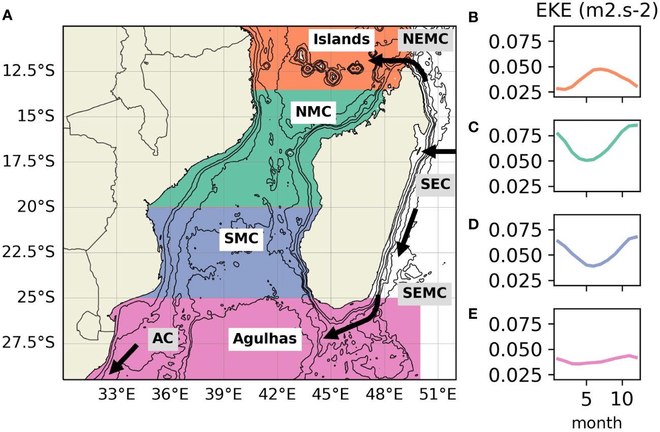
Figure 1 Major currents in the Mozambique Channel, its 4 subregions (A), and their respective EKE climatology (B–E). The subregions are defined in the text as “Islands” (10°S- 13.5°S), “North Mozambique Channel” (NMC: 13.5°S- 20°S), “South Mozambique Channel” (SMC: 20°S-25°S) and “Agulhas” (25°S-30°S). The major currents, South Equatorial Current (SEC), North East Madagascar Current (NEMC), South East Madagascar Current (SEMC) and the Agulhas Current (AC) are indicated by arrows. The background contours represent isobaths at -200, -1000, -2000, -3000 and -4000 m.

The MC also exhibits a strong seasonal cycle and experiences biannual monsoons north of 20°S (Schott et al., 2009). During the northeast monsoon, from December to March, winds blow from the northwest, while winds blow from the southeast during the southwest monsoon, from June to November. South of 20°S, winds blow from the southeast all year round (Obura et al., 2019). The monsoon reversals of the north MC also modulate currents intensity (Ridderinkhof et al., 2010; Obura et al., 2019) and create a distinct seasonal pattern, which affects the large anticyclonic eddies forming at 12-16°S (Donguy and Piton, 1991). Finally, altimetry-derived EKE climatology for different parts of the MC (Figure 1) shows a strong seasonal variability, especially north of 25°S. The MC energetic turbulent flow, seasonal cycle and exceptional biodiversity (Obura et al., 2019) thus motivate the investigation of temperature front seasonal variability.

Historically, fronts have mostly been detected from satellite imagery. Originally, fronts were simply identified manually from SST images (Legeckis, 1978), but more sophisticated automatic front detection algorithms have been developed since then. Front detection algorithms are usually based on SST gradients, even though some also use entropy (Shimada et al., 2005), neural networks (Torres Arriaza et al., 2003) or singularity exponents (Turiel and del Pozo, 2002; Turiel et al., 2008; Tamim et al., 2015). The Canny algorithm (Canny, 1986) is often referred to as the original “gradient method” and is based on the high gradient property of fronts. However, this method often results in enhanced noise from the differentiation (Belkin and O’Reilly, 2009). The Cayulla-Cornillon Algorithm (CCA) addresses this shortcoming by operating with histograms to detect the edge between two water masses (Cayula and Cornillon, 1995). This method requires fine-tuning to find the appropriate threshold distinguishing fronts from background noise, but has been successfully used in many different systems: in the Baltic Sea (Kahru et al., 1995), in the Atlantic Ocean (Mantas et al., 2019) or in the South China Sea (Wang et al., 2001). The performance of the CCA was further improved by adding multiple sliding windows (Nieto et al., 2012) and then applied in the Indian (Nieblas et al., 2014) and Pacific (Nieto et al., 2017) Oceans. As opposed to histogram-based methods, the algorithm proposed by Belkin and O’Reilly is based on SST gradients and effectively remove the noise generally produced by other gradient methods, while preserving the shape of the detected front (Belkin and O’Reilly, 2009). The Belkin and O’Reilly algorithm (BOA) produced fronts dataset in the South China Sea (Wang et al., 2001), East China Sea (Lin et al., 2019) and the Kuroshio current (Liu et al., 2018).

Fronts can originate from the interaction between strong currents and topography anomalies, such as shelf-breaks, islands and seamounts (Heywood et al., 1990; Condie, 1993; McWilliams, 2021); at the edge of eddies in turbulent areas (Munk et al., 2000; Read et al., 2007; Siegelman et al., 2020a) and in upwelling zones (Bettencourt et al., 2012; Rossi et al., 2013; Sabarros et al., 2014; Calil et al., 2021). The Island Mass Effect (Doty and Oguri, 1956) in particular plays an important role in frontogenesis, as it has been shown to be associated with the generation of vortices in the lee of islands (De Falco et al., 2022). Although it is very rare to attribute clearly a single driver to frontogenesis, it is instead often a complex combination of favorable conditions (McWilliams, 2021).

The complex dynamic of processes behind frontogenesis (McWilliams, 2021) suggests that fronts detection relying solely on remotely sensed SST might miss important front features and variability at depth, and estimates of the magnitude of SST gradients in satellite products is highly sensitive to resolution and interpolation technique (Vazquez-Cuervo et al., 2013). In this study, we use remotely-sensed SST and outputs of a high-resolution realistic ocean model to investigate the spatial and seasonal variability of thermal fronts at different depths in the Mozambique Channel. The paper is organized as follows: we first introduce our material and methods for front detection and we follow with a description of front variability in the Mozambique Channel. The article ends by a discussion and a few concluding remark

2. Material and methods

2.1. Domain subregions

Before studying thermal front variability, we divided our domain into 4 subregions, as seen in Figure 1. The rationale for this meridional subdivision is based on a literature review about drivers of oceanic variability (i.e. bathymetry effects, monsoon forcing) in the channel and relies on the dependence of eddy characteristics and therefore fronts to the Coriolis force. The “Islands” subregion (10-13.5°S, 38-49.5°E) starts just above the Comoros archipelago and extends to 13.5°S at the entrance of the Angoche Basin. The “Northern Mozambique Channel” (NMC) subregion (13.5-20°S, 34-48°E) ends at 20°S where the influence of monsoons weakens substantially (Schott et al., 2009). The “South Mozambique Channel” (SMC) subregion (20-25°S, 33-45°E) goes as far south as 25°S, which corresponds to the southern tip of Madagascar island. Finally, the “Agulhas” subregion (25-30°S, 31-50°E) covers the southernmost part of our domain from 25°S to 30°S.

2.2. Model configuration

In this study, temperature fronts are derived from a ROMS-CROCO (Regional Ocean Modeling System and Coastal and Regional Ocean COmmunity model) configuration of the MC (Shchepetkin and McWilliams, 2005). ROMS-CROCO solves the primitive hydrostatic equations for momentum and tracer variables and successfully resolves regional and coastal oceanic processes at high resolution, as well as mesoscale eddies (Halo et al., 2014). The model configuration consists in 3 nested grids (two-way nesting) with the child domain at the highest resolution of 1/36° used here. 60 vertical sigma (topography following) layers are used. The bathymetry used in the model is from GEBCO 2014 (Weatherall et al., 2015). A bulk formulation (Fairall et al., 1996) is used to compute surface turbulent heat to force the model, based on ERA-Interim Reanalysis daily mean atmospheric fields (2 m air temperature, relative humidity, surface wind speed, net shortwave and downwelling longwave fluxes, and precipitations). Wind stress forcing is also from the ERA-Interim Reanalysis. At the lateral open boundaries, mixed active-passive conditions are used (Marchesiello et al., 2001) with forcing data from GLORYS reanalysis at 1/4° resolution. The generated daily output covers 22 years, from 1993 to 2014. This 1/36° ROMS-CROCO configuration of the Mozambique Channel, referred to as MOZ36, was first used by Miramontes et al. (Miramontes et al., 2019) to document the deep oceanic circulation in the Zambezi turbidite system (SMC subregion in Figure 1)

2.3. Climatological and satellite datasets

We used climatological seawater properties from CARS2009 (Ridgway et al., 2002) generated from compiled in-situ observations spanning from January 1941 to May 2009, on a 1/2° grid. We also retrieved World Ocean Atlas 2018 annual mean temperature (Locarnini et al., 2018) and salinity (Zweng et al., 2018). Remotely-sensed Sea Surface Height (SSH) was taken from Global Total Surface and 15 m Current (Rio et al., 2014, COPERNICUS-GLOBCURRENT) from Altimetric Geostrophic Current and Modeled Ekman Current Reprocessing, on a 1/4° grid. Finally, Sea Surface Temperature (SST) was provided by GHRSST Level 4 Multi-scale Ultra-high Resolution (MUR) 1/10° Global Foundation Sea Surface Temperature Analysis v4.1 (SST MUR) (Chin et al., 2017). In this work, we use the full MUR dataset from January 2003 to December 2020, for the MC. SST MUR data comes with 2 data quality flags. Flag 1 corresponds to the estimated error standard deviation of the SST data and flag 2 is the time lag to most recent 1 km data. Flag 1 is available for the entire dataset while flag 2 is only included after July 2016.

2.4. Numerical methods

We use the Brunt-Väisälä frequency N as a proxy for stratification. N is given by:

$\begin{array}{ll}{\text{N}}^2=\frac{-g}{{\rho }_0}\frac{\partial \rho }{\partial z}& (1)\end{array}$

Where g is the gravitational constant, ρ₀ is a reference density set at 1025 kg.m^-3ρ is the seawater density and z its depth.

Intra-seasonal and inter-annual eddy kinetic energy (EKE) were computed following a similar method to Dewitte et al. (Dewitte et al., 2021). First, intra-seasonal current anomalies (u_IS and v_IS) were estimated by subtracting monthly mean currents to the daily velocity dataset. Then, the mean intra-seasonal EKE was computed as:

$\begin{array}{ll}\langle {\text{EKE}}_{\text{IS}}\rangle =\langle \frac{\left({\text{u}}_{\text{IS}}^2+{\text{v}}_{\text{IS}}^2\right)}{2}\rangle & (2)\end{array}$

Second, inter-annual current anomalies (u_IA and v_IA) were computed by subtracting the climatology to the daily velocity dataset. Then, the mean inter-annual EKE was computed as:

$\begin{array}{ll}\langle {\text{EKE}}_{\text{IA}}\rangle =\langle \frac{\left({\text{u}}_{\text{IA}}^2+{\text{v}}_{\text{IA}}^2\right)}{2}\rangle & (3)\end{array}$

Following the same methodology, MOZ36 intra-seasonal EKE was also computed at -100 m, -500 m and -1000 m.

We chose the Belkin and O’Reilly algorithm (Belkin and O’Reilly, 2009) to detect the location and intensity of temperature fronts in the MC. More specifically, we use Ben Galuardi’s BOA pseudo-code written in R and publicly available on https://github.com/galuardi/boaR (accessed on 19 May 2022). BOA first applies a contextual median filter until convergence to reduce noise originating from natural variability and artifacts. The algorithm then uses 3x3 kernel Sobel operator to compute the gradient magnitude (Belkin and O’Reilly, 2009). BOA temperature gradients were computed on MUR SST but also on MOZ36 temperatures between 0 and -1000 m, leveraging the fact that the model is not limited to the surface, as would be satellite datasets. From the surface to -300 m, the model outputs were interpolated on a 10 m vertical resolution grid, while below -300 m we use a resolution of 50 m.

We derive several statistics to characterize temperature fronts and to evaluate their variability. BOA being a gradient-based method of front detection, the algorithm produces a continuous field of temperature gradient magnitude, or front intensity in °C/km. As such, a threshold must be determined to define what is considered a front. Choosing a high threshold might prevent weak fronts from being recorded, while a weak threshold might blur any meaningful signal into noise. We thus define front pixels as pixels whose temperature gradient magnitude is equal or above the chosen threshold. We finally define the probability of front occurrence per month for each ocean pixel as the percentage of days when the gradient value qualifies as “front”, i.e. when the pixel gradient magnitude is over the threshold, over the total number of days for each month of simulation.

Finally, we computed sea level anomalies (SLA) from the mean MOZ36 sea-surface heights in order to link frontal activity with (sub)-mesoscale features in the MC. And dominant time-frequencies were studied based on 1-D discrete fast Fourier transforms (FFT) computed with the scipy.fft package.

2.5. Model validation

2.5.1. EKE

To validate MOZ36 (sub-)mesoscale structures on intra-seasonal and inter-annual time scales, we evaluated the mean eddy kinetic energy (EKE) derived from the model and remotely-sensed currents (see supplementary material Figure S1). The spatial EKE patterns are similar in both model and satellite data: the EKE is most intense on the western part of the MC and in its southern part, in the wake of the SEMC. Note that, the slightly higher EKE from the model could be well-explained by its higher resolution.

2.5.2. Hydrography

When comparing the SST variability in the MC from MOZ36 and from MUR SST (Figure S2), both datasets exhibit comparable seasonal and spatial SST patterns. Additionally, and to further validate seawater properties of MOZ36, we compared World Ocean Atlas 2018 temperature (Locarnini et al., 2018) and salinity (Zweng et al., 2018) annually-averaged vertical profiles on a meridional section at 42.125°E, in the center of the channel (Figure S3). Observed and modelled vertical profiles show good consistency, confirming that MOZ36 is suitable to study temperature fronts in the MC.

2.5.3. Stratification

We used CARS2009 (Ridgway et al., 2002) temperature and salinity profiles to evaluate the realism of the modelled vertical stratification thanks to the Brunt-Väisälä frequency from the surface to -1000 m. The comparison between the mean model and CARS2009 squared Brunt-Väisälä frequencies for the 4 MC subregions (Figure S4) reveals that MOZ36 is able to reproduce a range of values similar to observations, with a maximum N² of about 0.2*10^-3s^-2. For both datasets, N² in the Agulhas region is markedly smaller than the other 3 subregions and peaks at -60 m. The Islands, NMC and SMC subregions peaks between -60 and -100 m in the model and between -80 and -125 m in CARS2009. Overall the model reproduces a rather realistic mean thermocline structure, providing high confidence in its ability to simulate well the main aspects of ocean dynamics.

3. Results

3.1. Front threshold definition

We define a single temperature front threshold for all depths using statistical distribution and quantiles of MOZ36 temperature front intensity for all ocean pixels across the 22 years of simulation and 4 depth levels: surface, -100 m, -500 m, and -1000 m (Figure S5). Surface temperature gradients go up to 2.3°C/km, and 70% of those are below 0.05°C/km. We subsequently define front pixels as pixels whose temperature gradient magnitude is equal or above 0.05°C/km, and the probability of front occurrence per month for each ocean pixel as the percentage of days when the pixel gradient magnitude is over 0.05°C/km, over the total number of days for each month of simulation.

3.2. Spatial variability

3.2.1. Surface

The mean surface temperature front intensity and probability maps (Figures 2A, B) reveals that SST fronts derived from the model are more intense and more likely to appear along the continental shelves, in the wake of both Northeast and Southeast Madagascar currents (NEMC and SEMC) and more generally southward of 25°S.

FIGURE 2

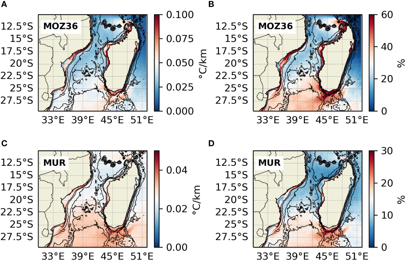
Figure 2 Mean surface temperature front intensity (A, C) and probability (B, D) for MOZ36 (A, B) and MUR SST (C, D).

The equivalent mean maps of temperature front intensity and probability derived from the MUR dataset exhibit a spatial distribution similar to that of the modelled fronts (Figures 2C,D), despite a slightly lower range of values.

3.2.2. Ocean interior

Figure 3 represents the mean vertical profiles of front intensity in °C/km from MOZ36, the shading around the mean corresponds to the seasonal standard variation. The vertical profiles reveal three distinct regimes, similar in all 4 subregions of the MC:

1. From the surface to about -100 m, the frontal activity increases abruptly to reach its maximum to 0.75-0.9°C/km at -100 to -200 m, in the vicinity of the mean thermocline.

2. From -200 m to -500 m, the front intensity decreases sharply to reach 0.35°C/km in the NMC region and around 0.05°C/km in the Islands, NMC and Agulhas regions.

3. From -500 m and deeper, frontal intensities decrease at a slower rate with depth. At -1000 m the NMC region exhibits the lowest frontal activity, followed by the Islands regions. The SMC and the Agulhas region show less of a vertical difference between surface and depth, than the NMC and the Islands regions.

FIGURE 3

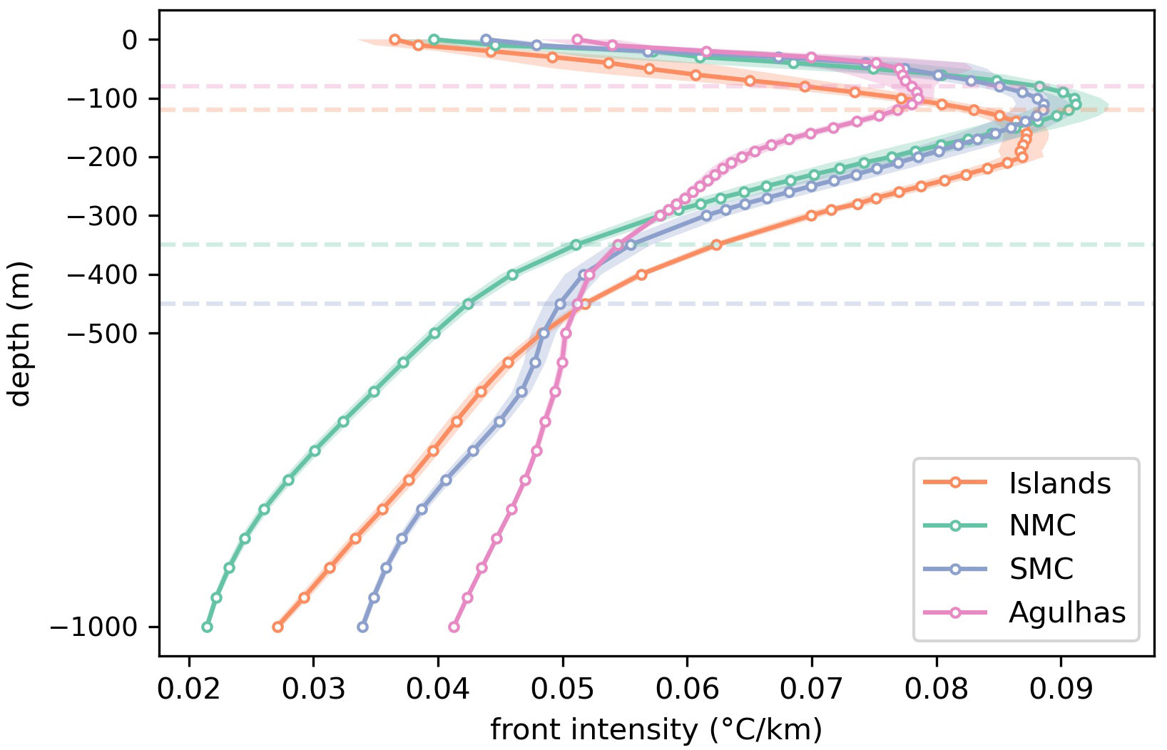
Figure 3 Mean temperature front intensity for each MOZ36 subregion in °C/km. The shading shows the seasonal standard deviation from the mean. The dashed horizontal lines mark the depth below which the seasonal standard deviation of temperature front intensity is lower than 5% of its mean.

The vertical distribution of temperature front intensity is very similar to MOZ36 and CARS2009 stratification profiles (Figure S4). Indeed, the Islands (Agulhas) subregion has the deepest (shallowest) thermocline and frontal intensity peak, at about -200 m (-80 m).

Seasonal variability ceases to be significant, i.e. it amounts to less than 5% of the front intensity mean, below -150 m for the Islands region, below -350 m and -450 m for the NMC and SMC regions (respectively) and below -70 m in the Agulhas region.

Frontal activity peaks at around -100 m, in the vicinity of the mean thermocline (Figure 3). The resulting 22-year map of mean front intensity at -100 m (Figure 4C) indicates stronger frontal activity than at the surface, as expected from the front intensity distribution (Figure S5). The frontal activity is specifically stronger along the continental shelves, in the wake of the NEMC and SEMC and in the central part of the MC, in between Bassas da India and Juan de Nova islands across the Angoche Basin.

FIGURE 4

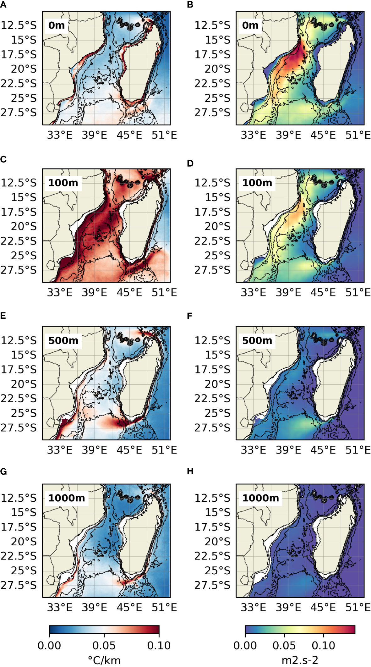
Figure 4 Mean temperature front intensity (A, C, E, G) and EKE (B, D, F, H) from MOZ36 at the surface (A, B), -100 m (C, D), -500 m (E, F) and -1000 m (G, H).

-500 m and -1000 m temperature fronts are most intense along the Mozambican shelf, near Maputo and in the path of the NEMC and SEMC (Figure 4).

3.2.3. Front typology

Selected snapshots of temperature front intensity at different depth and time of the year allowed us to distinguish three types of temperature fronts based on their signature behaviors (Figure 5).

● Topographic fronts, as defined by McWilliams McWilliams (2021) are formed where currents encounter land masses or other sharp topographic changes such as seamounts. In this study, topographic fronts are found along Mozambique and Madagascar shelves and around islands (French Scattered Islands, Comoros Archipelago), they reach maximum intensity at -100 m. NEMC and SEMC paths can clearly be identified from the front intensity patterns at the north and south tips of Madagascar Island (Figure 4).

● The next two types of fronts correspond to the “deformation fronts” in McWilliams’s typology. They form at the edge of eddies.

1. • Anticyclonic deformation fronts (ADF) are located at the edge of anticyclonic eddies (AE) in the MC. AE usually form at the entrance of the Angoche Valley at 15°S and travel southward close to the Mozambican shelf to then merge or dissipate around 22°S and feed the Agulhas Current. ADF reach their maximum intensity at around -100 m and then weaken substantially at -500 m, to disappear completely by -1000 m.

2. • Cyclonic deformation fronts (CDF) form at the edge of cyclonic eddies (CE), generally south of 23°S. Most of those CE are driven by the SEMC: some go slightly northward up the southern tip of the Madagascar shelf, but most go southwest following the SEMC track towards the Agulhas current. CDF reach their maximum intensity at -500 m and can still be detected at -1000 m.

FIGURE 5

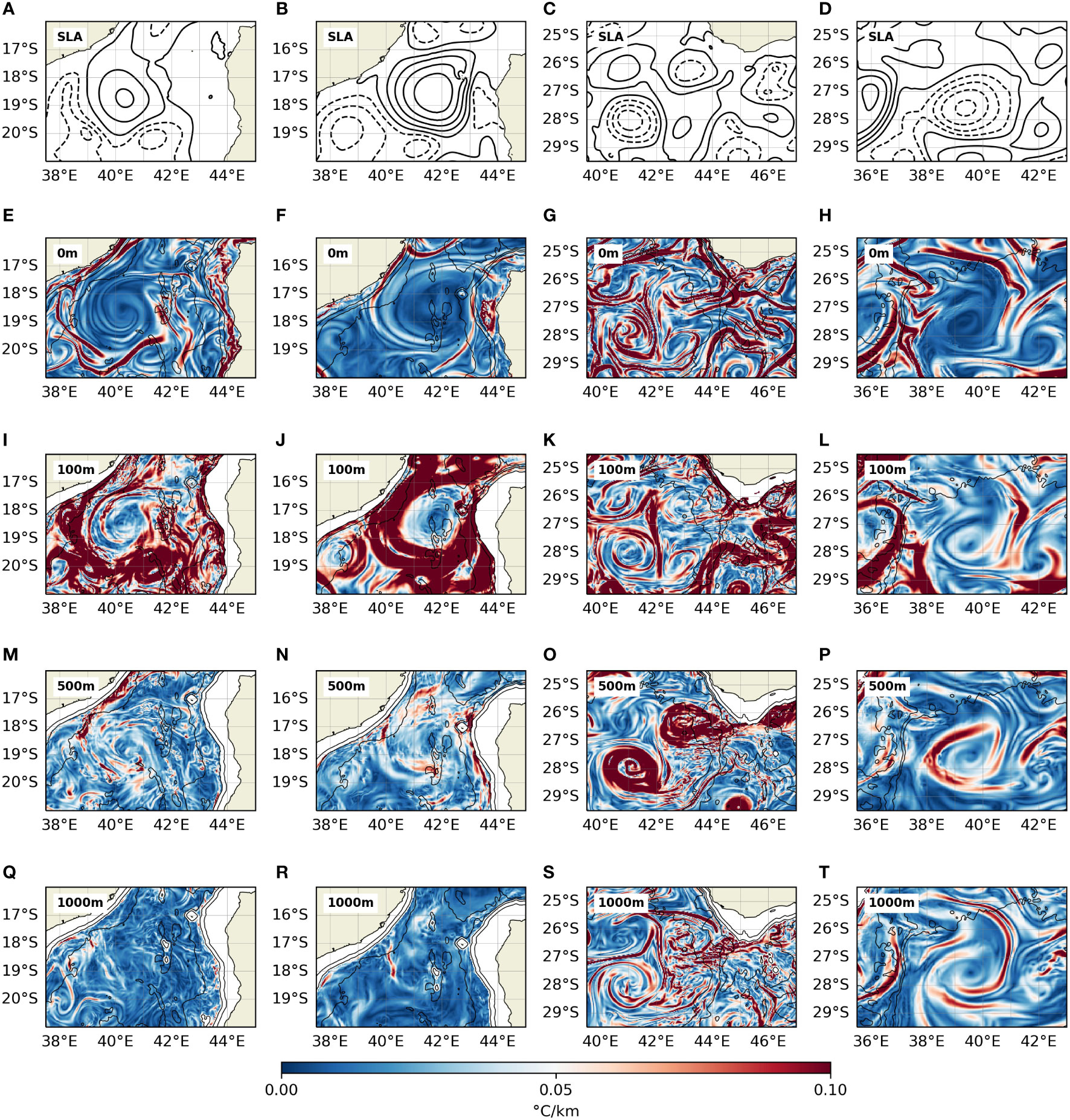
Figure 5 Selected snapshots comparing the vertical structures of anticyclonic (first 2 columns: A, B, E, F, I, J, M, N, Q, R) and cyclonic (last 2 columns: C, D, G, H, K, L, O, P, S, T) eddies from MOZ36. Each column represents a different eddy structure. The first row corresponds to sea-levels anomalies relative to mean sea-surface height, full (dashed) lines are positive (negative) anomalies. Rows 2, 3, 4 and 5 are temperature front intensities in °C/km, at surface, -100 m, -500 m, -1000 m respectively.

A summary of the front typology and locations can be found in Table 1.

TABLE 1

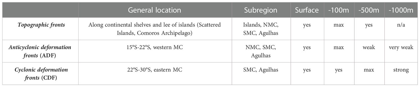
Table 1 Front typology based on behavior and depth signatures.

3.3. Seasonal variability

3.3.1. Islands and NMC subregions

In the Islands (10°S-13°S) and NMC (13°S-20°S) regions, SST fronts are strongest in the wake of the NEMC between the northwestern tip of Madagascar and the Comoros archipelago (Figure 4) and along the Madagascar and Mozambican continental shelves. Most of the fronts in the Islands region are identified as topographic fronts, generated by the interaction between NEMC and the local topography, while fronts in the NMC are mostly topographic fronts and ADF. The FFT analysis of the 22-year daily time series of surface temperature front intensity from MOZ36 in the Island and NMC regions reveals a predominant 6-month and a moderate 1-year periods (Figure 6, additional depths are provided in supplementary material (Figure S6). Indeed, SST front intensity climatology shows two peaks: a moderate one in May and a greater one in November (Figure 7).

FIGURE 6

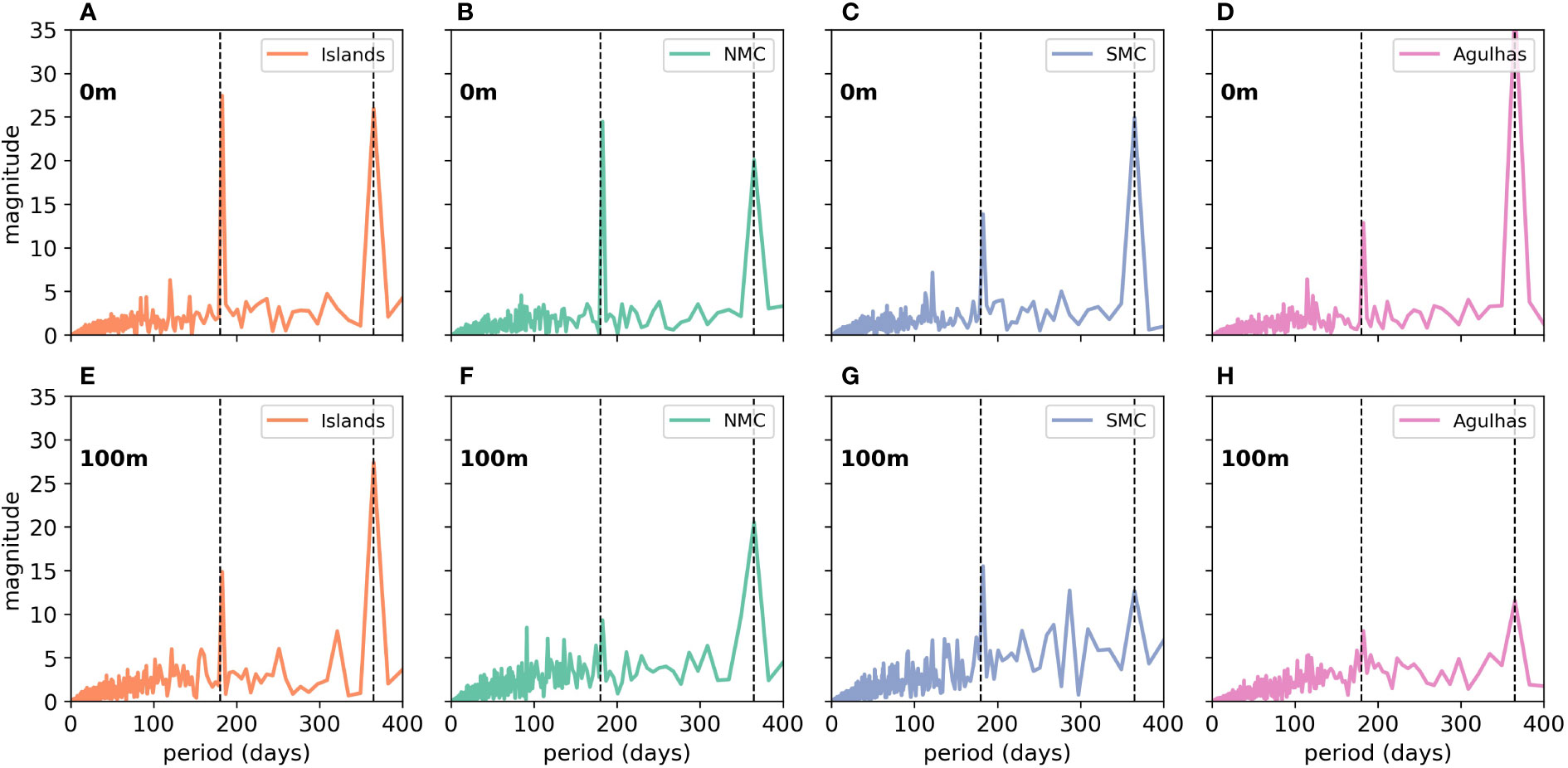
Figure 6 Fast Fourrier Transform analysis periodograms of MOZ36 front intensity in the 4 subregions: Islands (A, E), NMC (B, F), SMC (C, G), Agulhas (D, H) and at two depths: surface (A-D), -100 m (E-H). The dashed vertical lines represent periods of 6 and 12 months. -500 m and -1000 m periodograms are not shown here because they did not show any significant magnitude peak, they are available as Supplementary Material, Figure S6.

FIGURE 7

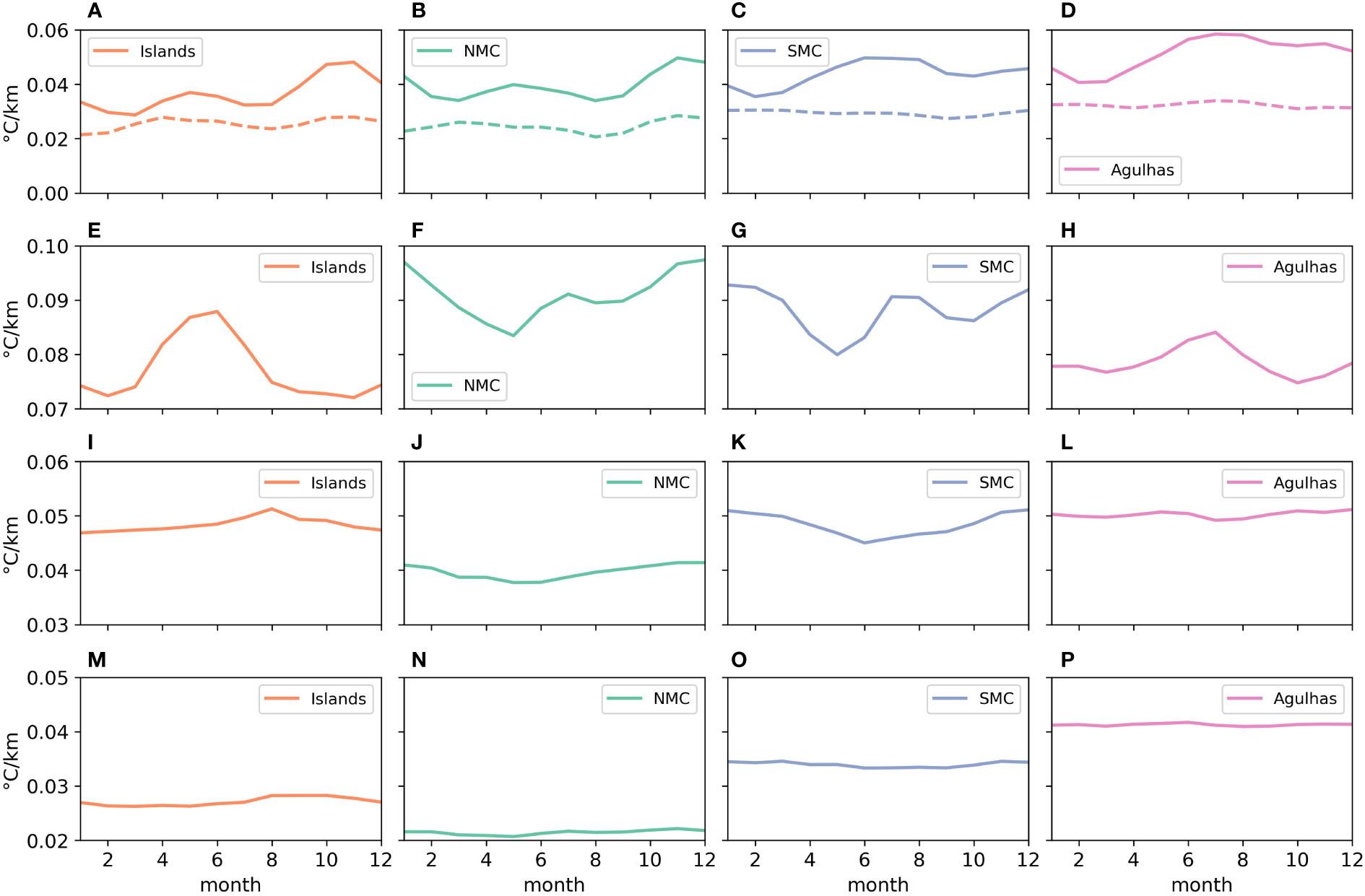
Figure 7 Temperature front intensity climatology for each subregion at surface (A-D), -100 m (E-H), -500 m (I-L), -1000 m (M-P). At surface (A-D), data from MOZ36 (full line) and from SST MUR (dashed line) are represented. Please note the different y axis range.

Note that the surface climatology of front intensity from MUR SST (Figure 7) shows little seasonal variability compared to the model. This aspect is explored later in the discussion part, where quality flags explain well why the seasonal cycle is significantly dampened compared to the model.

In the Islands subregion, the -100 m front intensity is greater than at the surface and peaks in late austral autumn (June). The signature 2-peak of the surface signal seems to have disappeared entirely, leaving only one clear maximum in winter. In the NMC area, the -100 m front intensity is higher than at the surface and peaks in austral summer, with a second local maximum in austral winter. At -500 m and -1000 m, there is not much seasonal variation anymore (Figure 7).

3.3.2. SMC and Agulhas subregions

In the SMC (20°S-25°S) and in the Agulhas (25°S-30°S) subregions, surface temperature fronts are more intense along the continental shelves and in the wake of the SEMC. The FFT analysis of the 22-year daily time series of SST front intensity from MOZ36 in the two southernmost regions reveals both 6-month and 1-year periods, but this time the yearly signal exhibits stronger magnitude than the biannual one (Figure 6). The climatology of surface temperature front intensity (Figure 7) shows stronger frontal activity during austral winter and spring, with a slight increase in December in the SMC.

Similarly to the NMC, the -100 m temperature front climatology in the SMC is stronger than at the surface and reveals two local maxima with comparable range, in austral summer and winter (Figure 7). In the Agulhas region, the -100 m front climatology (Figure 7) shows a much weaker seasonal variation, also seen on the FFT analysis (Figure 6), with a slight maximum in austral winter.

At -500 m and -1000 m, little seasonal variation is seen in frontal activity (Figure 7). However, even though the fronts become less intense with depth, -500 m and -1000 m fronts in the SMC and Agulhas subregions are still more intense than in the Islands and NMC regions. Indeed, the interaction between the SEMC and local topography fosters the formation of cyclonic eddies and thus of CDF, which have shown to have a strong deep signature in the model (Figure 5).

4. Discussion

4.1. Data and method

The extended MOZ36 validation process conducted in this work and in Miramontes et al. (2019) has confirmed its suitability in depicting realistic basin-scale and regional dynamics of the MC. Yet, the temperature front seasonal variability exhibited by MUR SST data does not match perfectly MOZ36 results, despite consistent spatial patterns. This disparity can be explained by MUR SST cloud cover adjustments. A preliminary comparative study between MUR SST flags values and corresponding BOA temperature front intensity revealed that periods with higher cloud cover (mostly during austral summer) resulted in dampened frontal activity: the frontal structures are less sharp or non-existent, and the gradient magnitudes much less intense. These higher cloud cover areas correspond to flag 1 values being above 0.39°C and flag 2 values being above 20 hours. For example, Figure 8 shows snapshots of front intensity (C, D) and corresponding flag 1 (E, F) and flag 2(G, H) for the first day of February and July 2020. One can distinctively see a difference in Figure 8C between the Mozambique shelf north of 17°S where fronts are dimmed, and the center of the MC at around 20°S, where the structures are much sharper. The top panels of Figure 8 show the climatology of monthly percentage of ocean pixels having acceptable flag values to study frontal activity, based on flag 1 for 2003-2020 (Figure 8A) and on both flags for 2017-2020 (Figure 8B). If we only take flag 1 into account, 50-90% of the dataset is acceptable, while if we consider both flags then only 10-50% of the dataset is suitable to study seasonal variability of submesoscale fronts in the MC. Regardless of how many flags are considered, a bigger proportion of pixels are not suitable in austral summer, compared to austral winter, providing a good explanation as to why so little seasonality is seen from MUR SST front intensity in Figure 7. Indeed, the difference between seasons in frontal activity could be significantly dampened by the cloud cover. Additionally, the seasonality in mean EKE is comparable between observations (altimetry) and the model (not shown), which also suggests the limitations of the MUR dataset.

FIGURE 8

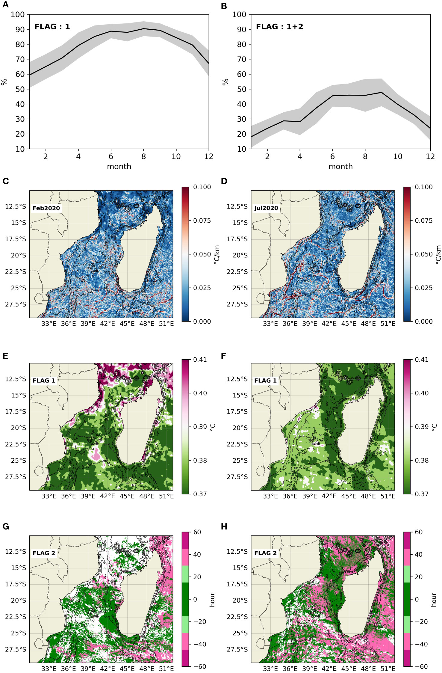
Figure 8 The first row represents the climatology of the percentage of pixel deemed of a sufficient quality for frontal analysis based on: flag 1 for 2003-2020 (A); or flag 1 and flag 2 for 2017-2020 (B). The grey shaded area is the standard deviation from the climatology mean. The 2nd row shows temperature front intensity snapshots for February (C) and July (D) 1st, 2020. The 3rd and 4th row correspond to the same dates as the 1st row and show the corresponding flag values: flag 1 (E, F) and flag2 (G, H).

Other tracer-based front detection algorithms, such as the objective Cayulla Cornillon Algorithm (Cayula and Cornillon, 1995) and the Nieto method (Nieto et al., 2012), could have been used to detect temperature fronts in the MC, but they do not provide gradient magnitudes. Moreover, we did find a temperature front intensity threshold and spatial variability similar to what is documented in Nieblas et al. (2014), despite using a different front detection algorithm.

Finally, it would be interesting to use Lyapunov Exponents as in Hernández-Carrasco et al. (2012); Bettencourt et al. (2012) and Siegelman et al. (2020b; 2020a) to bring a dynamic-based approach to our multidecadal tracer-based front database.

4.2. Spatial variability

We have leveraged the 3D component of the well-validated MOZ36 to go beyond the surface and explore temperature front activity in the MC ocean interior as well. To our knowledge, this is the first temperature front spatial and seasonal variability analysis extending to the ocean interior in the MC.

The mean maps of frontal intensity and probability (Figure 2) from MOZ36 and MUR SST present similar spatial patterns to what is shown in Nieblas et al. (2014). Additionally, the vertical distribution of temperature front intensity is consistent with the stratification profiles from MOZ36 and CARS2009 (Figure S4). Indeed, the Islands (resp. Agulhas) region has the deepest (resp. shallowest) thermocline and frontal intensity peak, at about -200 m (-80 m). It is worth noting that as MOZ36 does not consider the run-off from the Zambeze river, we expect thermal shelfs fronts over the SofalaBank to be underestimated. In all 4 regions, front intensity is maximum at around -100 m, in the vicinity of the mean thermocline. The maximum intensity fronts at around -100 m may be explained by strain-induced vertical velocities at the edge of eddies, which intensify below the mixed layer and up to -400 m below it (Keppler et al., 2018; Siegelman et al., 2020a).

ADF develop at the border of large anticyclonic eddies, or Mozambique Rings, on the western side of the MC, as observed by Biastoch and Krauss (1999) and Schouten et al. (2003). On the other side of the channel, CDF form at the edge of smaller cyclonic eddies, mostly on the southeastern side of the channel and driven by the SMEC, as seen in Gründlingh’s work (Gründlingh, 1995). In MOZ36, the temperature front signature of the anticyclonic Mozambique Rings seems to be limited to the upper layers of the water column. However, some discrete observations (de Ruijter et al., 2002) and MOZ36 modelled current (Miramontes et al., 2019) have shown that the dynamics of the Mozambique Rings could indeed reach the bottom. It is still unclear why the temperature front signature of these anticyclonic rings remains weak below 500 m while their associated currents have been previously reported at much deeper levels in the model.

4.3. Seasonal variability

Our EKE mean maps (Figure 4) and seasonal variability analysis (Figure 9) in the MC are consistent with Martínez-Moreno et al. (2022) work on EKE seasonality in the Southern Hemisphere.

FIGURE 9

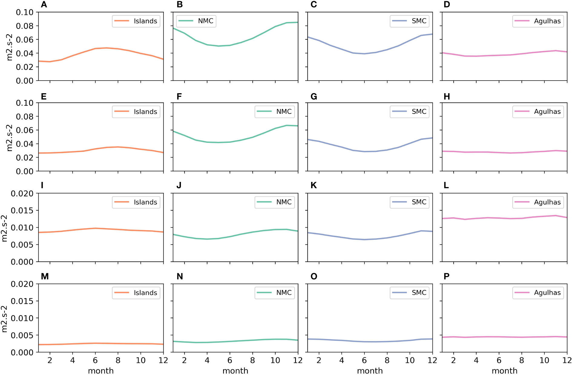
Figure 9 MOZ36 EKE climatology for each subregion at surface (A-D), -100 m (E-H), -500 m (I-L), -1000 m (M-P). Please note the different y-axis range.

Seasonal variability in the MC ceases to be significant below -150 m for the Islands subregion, below -350 m and -450 m for the NMC and SMC subregions (respectively) and below -70 m in the Agulhas subregion (Figure 3). This is aligned with the types of fronts that characterize each subregion, as summarized in Table 1. The NMC and SMC subregions are eddy-rich subregions generating mostly ADF and CDF fronts which are more likely to reach deeper in the water column than topographic fronts, and thus propagate surface seasonal signals at depth. We suspect this explains why the seasonal variability in the NMC and SMC subregions reaches deeper layers in the water column. Potential drivers of the seasonal variability for each region are summarized in Table 2.

TABLE 2

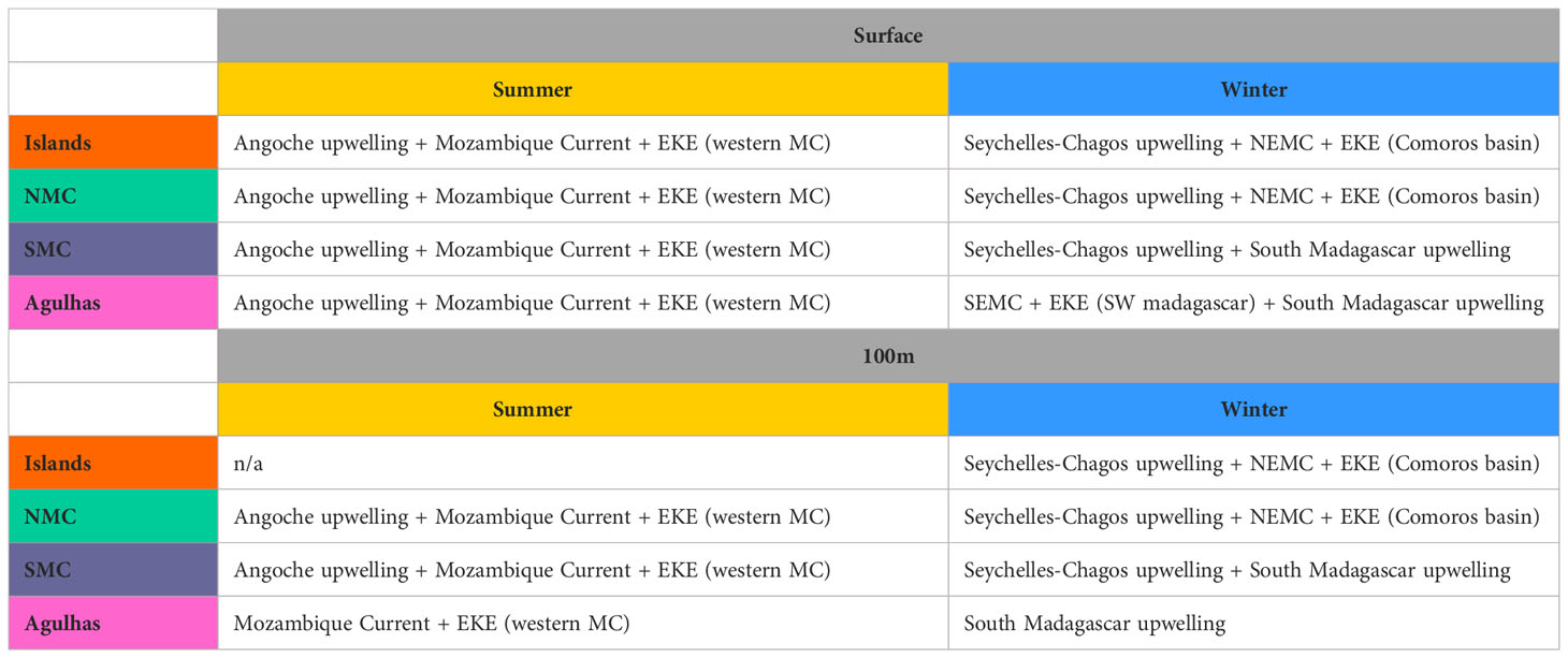
Table 2 Summary of the main drivers of thermal front seasonal variability in the Mozambique Channel, at surface and -100 m.

4.3.1. Islands and NMC subregions

In the Islands and NMC regions, SST front intensity climatology shows two local maxima: a moderate one in May and a greater one in November (Figure 7). A similar semi-annual cycle at the Seychelles Chagos thermocline ridge (Hermes and Reason, 2008) suggests that the Seychelle-Chagos upwelled waters might be one of the possible drivers of temperature front seasonal variability at the surface of both northernmost regions. Additionally, the presence of “cool water” events near Angoche during August to March (Malauene et al., 2014), and upwelling along the Mozambican coast at 11-16°S during the North East monsoon (November-March) (Sætre and Da Silva, 1984) could explain the higher intensity of the second peak in austral spring and summer, especially in the NMC. Another driver behind the local winter maximum could be the elevated EKE in this area responding to the seasonal increase of the NEMC (Figure 9) (Obura et al., 2019).

In the Islands subregion, the -100 m front intensity is greater than at the surface and peaks in late austral autumn. The signature 2-peak of the surface signal has disappeared entirely, leaving only one clear maximum in May-June (Figure 7). This suggests that the -100 m fronts may not be driven by the same processes than the surface ones. Since most fronts in the Islands region belong to the topographic class, and since the NEMC peaks in austral winter (Obura et al., 2019), -100 m temperature fronts in the Islands region seem to be driven solely by seasonal variations of the NEMC and its subsequent interactions with the local topography.

In the NMC area, the -100m front intensity is higher than at the surface and peaks in austral summer, with a second local maximum in austral winter (Figure 7). Those two peaks can be explained by the types of front predominantly found in this region: topographic fronts, and especially ADF (Table 1). On the first hand, as seen in the Islands subregion, topographic fronts follow the variability of the NEMC, which is stronger in austral winter (Obura et al., 2019), explaining the winter peak of frontal activity. On the other hand, ADF are shaped at the edge of anticyclonic eddies forming in this region (Schouten et al., 2003; Halo et al., 2014) and are thus likely linked to variations of EKE, which would explain the frontal activity maximum in austral summer, coinciding with peaks of EKE (Figure 9)

At -500 m and -1000 m, there is not much seasonal variation anymore and frontal activity weakens with depth (Figure 9). This is consistent with our preliminary front typology since ADF and topographic fronts, which represent the majority of fronts in Islands and NMC regions, have been found to present a weak deep signature.

4.3.2. SMC and Agulhas subregions

The FFT periodograms of the two southernmost subregions show that the yearly signal is stronger than the biannual one (Figure 6). The weaker biannual signal can be explained by the lesser influence of the monsoon below 20°S (Schott et al., 2009). The climatology of surface temperature front intensity in the SMC and Agulhas regions (Figure 7) shows stronger frontal activity during austral winter and spring which coincides with upwelling cells at the southern tip of Madagascar driven by the SEMC (Ho et al., 2004; Ramanantsoa et al., 2018) and the local winds (Lutjeharms and Machu, 2000; DiMarco et al., 2000). Frontal activity in the SMC and Agulhas regions also show a slight increase around December (Figure 7). One possible explanation is the Angoche upwelling cell, which brings cooler water to the surface in austral summer (Malauene et al., 2014). Another possible driver could be the eddy activity, which peaks in austral summer in these regions. Indeed, since the SMC and Agulhas regions seems to host mostly CDF and topographic fronts, it is likely that the temperature front variability in these regions depends on EKE variability.

In the SMC at -100m depth, the first local maximum in austral summer (Figure 7) coincides with a -100 m EKE peak (Figure 9), which suggests that frontal activity there is driven by MC eddies. The second peak in austral winter can be attributed to the local upwelling cells south of Madagascar island (Ramanantsoa et al., 2018), which was also the main driver of surface frontal activity in this region. In the Agulhas region, the -100 m front climatology (Figure 7) shows much weaker seasonal variation, also seen on the FFT analysis (Figure 6), with a slight maximum in austral winter, when the South Madagascar upwelling cells are most active (Ramanantsoa et al., 2018). The absence of austral summer peak, like it is observed in NMC and SMC, can be explained by the comparably weaker EKE seasonal variations in the Agulhas region (Figure 9). It is worth noting that the FFT analysis (Figure 6, and Figure S6) does not show a clear annual or bi-annual period for the SMC and Agulhas regions from -100 m depth and below, which could be linked to the higher inter-annual variability observed in this region (Palastanga et al., 2006).

-500 m and -1000 m fronts in the SMC and Agulhas subregions are more intense than in the Islands and NMC at the same depth, possibly due to the specific typology of fronts most often encountered in the south MC (Table 1). In the SMC and Agulhas, the majority of fronts belong to the CDF category, which have a stronger depth signature, hence the greater -500 and -1000 m front intensity compared to regions where ADF dominate.

Finally, a modest peak at about 4-month can be identified in the FFT analysis periodograms (Figure 6), especially at the surface of the Islands, SMC and Agulhas subregions. This could be attributed to Indian Ocean basin resonance characterized by 120-day period, as detected by both idealized and realistic models (Han et al., 2011).

4.4. Main drivers of frontogenesis in the MC

We have thus documented thermal front seasonal variability in the MC. The next section addresses the relative importance of the main drivers of frontogenesis in the region. A clear distinction between those physical processes would require carrying dynamical diagnostics such as eddy kinetic budgets [e.g., Conejero et al. (2020)], eddy kinetic energy decompositions [e.g., Martínez-Moreno et al. (2019; 2022] or frontogenesis function decompositions [e.g., Koseki et al. (2019)] based on the model outputs, which would fall beyond the scope of this work. We nonetheless argue that thermal fronts in the MC depends on mean and seasonal circulation, seasonal upwellings and variations of EKE. To do so, we first define our seasonal division: In the Mozambique Channel monsoon reversals occur first in April to June and then in October to November, marking the separation between winter and summer (Collins, 2013; Obura et al., 2019). We thus define winter as the period from April to September, and summer as the period from October to March.

4.4.1. Mean circulation

We can infer the role of the mean circulation on thermal front intensity (especially on the quasi-permanent fronts since no seasonal variability is involved here) from mean maps of surface current (northward and eastward velocities) and SST generated by the MOZ36 configuration (Figure S7). From the mean SST map (Figure S7.B), we can observe a strong thermal front at the northern tip of Madagascar, following the path of the North East Madagascar Current (NEMC), also visible in the mean current map (Figure S7.A) and the mean thermal front intensity (Figure 2). Similarly at the southwestern tip of Madagascar, a strong thermal front follows the path of the South East Madagascar Current (SEMC) toward the Agulhas current. Additionally, we can identify along-shelf thermal gradients of moderate intensity at the southeastern tip of Madagascar and off Maputo (Delagoa Bay), which are probably due to quasi-permanent coastal upwelling cells (Ramanantsoa et al., 2018), as well as a colder tongue extending along the outer parts of the Sofala Bank, which could be indicating the presence of a quasi-permanent shelf-break upwelling there, as documented by Hill and Johnson (1974); Gibbs et al. (2000) and Rossi et al. (2010).

4.4.2. Seasonal upwellings

Seasonal upwelling cells such as the Seychelles-Chagos upwelling (Hermes and Reason, 2008), the Angoche upwelling (Malauene et al., 2014) and, to a lesser extent, the South Madagascar upwelling cells (Ramanantsoa et al., 2018) mentioned in this work are strongly localized in space and time. The Seychelles-Chagos upwelling turns on in austral winter (Hermes and Reason, 2008), while the Angoche upwelling is active during the August-March period (Malauene et al., 2014). The first upwelling core south of Madagascar is present all year round but reaches its maximum at the end of austral winter, while the second (much weaker) core is most active from October to January (Ramanantsoa et al., 2018). In the Islands and NMC regions, the mean thermal front intensity peaks first in May-June (Figure 7), which corresponds to the first active period of the Seychelles-Chagos upwelling system. This front intensity peak is mostly felt in the Islands subregion which is closest to the Seychelles-Chagos upwelling cell. We thus postulate that this first front intensity peak at surface and -100 m depth in both Islands and NMC subregions depends on the Seychelles-Chagos upwelling system. The second peak of frontal intensity in the same two northern subregions happens in November-December (Figure 7), and especially in the NMC region. We argue that this second peak is driven first by the Angoche upwelling and to a lesser extent by the Seychelles-Chagos upwelling. The seasonality of this second peak coincides with the Angoche most active period, which is located in the NMC, and the second (weaker) upwelling maximum in the Seychelles-Chagos located further upstream. The South Madagascar upwelling cells reach their maximum in winter, when the thermal front intensity peaks in both NMC and Agulhas subregions Figure 7). It thus suggests that the South Madagascar upwelling cells play an important role in the increased front intensity documented in the southernmost subregion during winter.

4.4.3. Seasonal current and EKE variability

Some quasi-permanent thermal fronts are found in the path of the NEMC, the SEMC and the Mozambique Current. The seasonal variability of these currents induces in turn variability of instabilities. We suggest that these instabilities, in turn, produce the sub to mesoscale activity that affects the intensity of those thermal fronts. The NEMC, and the EKE associated to its instabilities, are both stronger in winter (Figure S8 and S9), which also corresponds to a higher thermal front intensity in the northern Islands subregion, especially at -100 m (Figure S10 and S11). The Mozambique Current and the EKE in the western MC are stronger in summer (Figure S8 and S9), which also corresponds to higher thermal front intensity in the western half of the MC, especially in NMC and SMC subregions (Figure S10 and S11).

Finally, the suspected main drivers of seasonal variability of thermal front intensity, for each season and each subregion, and at both surface and -100 m, are summarized in Tables 2 and Table S1.

5. Conclusion and perspectives

We presented here the first thermal front seasonality analysis in the Mozambique Channel from the surface down to -1000 m depth. This work demonstrates that front dynamics in the MC are complex, and we suggest several possibilities to link temperature front seasonal variability to regional and remote ocean dynamics. Temperature fronts are generally more intense and more likely to occur over continental shelves, in the wake of the NEMC and SEMC, on the lee of islands, and at the edge of eddies. We show that temperature front intensity peaks below the mixed layer, between -100 and -200 m depth, which indicates that they are largely associated to aspects of the ocean dynamics rather than to mixed-layer processes. This consistent with the energetic mesoscale dynamics in this region.

Seasonal variations are felt down to -150 m in the Islands subregion, -350 m and -450 m in the NMC and SMC subregions (respectively) and -70 m in the Agulhas subregion. We argue that the main drivers of thermal front seasonal variability in the MC are upwelling cells (Angoche, South Madagascar, Seychelles-Chagos), current seasonal variability (NEMC, SEMC, and the Mozambique Current) and variations in EKE.

Since the MC circulation is connected to equatorial circulation in the Indian ocean, it is expected that temperature fronts experience fluctuations at interannual timescales. The Indian Ocean Dipole (IOD) seems to affect the variability of the transport (Ridderinkhof et al., 2010) and the SSH in the channel (Palastanga et al., 2006) through planetary wave propagation. A positive (negative) IOD event is linked to a weaker (stronger) NEMC (Ridderinkhof et al., 2010) which could potentially affect the intensity of fronts in the Islands and NMC subregions through fluctuations in current instabilities. Additionally, a change in SSH would also modulate the interactions between currents at the entrance or within the MC, which affects not only the EKE in the MC (Palastanga et al., 2006) but also the production of temperature front at the edge of eddies.

Another relevant path of investigation is suggested by Martínez-Moreno et al. (2021) in their global multidecadal study on altimetry and SST satellite-based observations. Their analysis shows that, even though SST gradients in the northern part of the MC have generally weakened between 1993 and 2020, the EKE has significantly increased during the same period in the northern MC and decreased in the southwest MC. This multidecadal trend suggests that climate change could have a significant impact on eddy-driven frontogenesis in the channel, as temperature fronts could be weaker but more numerous. Li et al. (2020) have also demonstrated a significant increase of stratification over the past half-century in the MC, especially in the Islands and NMC subregions. This suggests a possible enhancing of frontal activity due to climate change, especially in the two northernmost subregions, yet to be studied.

Thermal fronts, within and below the mixed layer, are thought to create transitory biodiverse hotspots across all trophic levels. Our analyses of their variability sheds light on where and when they are the strongest, with each subregion behaving differently. Altogether, it provides critical insights about where, horizontally and vertically, it is more relevant to survey bio-physical interactions and to consider protection initiatives in the MC. Conservation stakeholders could indeed use our synthetic analyses of front spatial and seasonal variability to elaborate rules for an adaptive and dynamic management of both epipelagic and mesopelagic realms, as also suggested in Brito-Morales et al. (2020) work on climate velocities. More research is needed to better apprehend climate change implications for front variability and their associated biological impacts to design an effective and climate-resilient network of pelagic and coastal marine reserves in the MC.

Data availability statement

The raw data supporting the conclusions of this article will be made available by the authors, without undue reservation.

Author contributions

FS with VR, BD, and VG designed the study. PP provided MOZ36 model output, and guidance for model analyses. JS retrieved the remotely sensed MUR SST data. FS produced the front database and subsequent analysis of the results. CM assisted with the High Performance Computing. VR, BD, and VG supervised the findings of this work and provided critical feedbacks. FS produced the figures and wrote the manuscript with input from all authors. All authors contributed to the article and approved the submitted version.

Funding

The authors acknowledge funding from the “Ocean Front Change” project, funded by the Belmont Forum and implemented through the French National Research Agency (ANR-20-BFOC-0006-04).

Acknowledgments

This work was supported by the Mediterranean Institute of Oceanography (MIO) and the French National Institute for Sustainable Development (IRD). The authors wish to thank J. Lecubin and C. Yohia for technical assistance with the local high performance computers and two reviewers for their helpful and constructive comments.

Conflict of interest

The authors declare that the research was conducted in the absence of any commercial or financial relationships that could be construed as a potential conflict of interest.

Publisher’s note

All claims expressed in this article are solely those of the authors and do not necessarily represent those of their affiliated organizations, or those of the publisher, the editors and the reviewers. Any product that may be evaluated in this article, or claim that may be made by its manufacturer, is not guaranteed or endorsed by the publisher.

Supplementary material

The Supplementary Material for this article can be found online at: https://www.frontiersin.org/articles/10.3389/fmars.2022.1045136/full#supplementary-material

References

Acha E. M., Mianzan H. W., Guerrero R. A., Favero M., Bava J. (2004). Marine fronts at the continental shelves of austral south america. J. Mar. Syst. 44, 83–105. doi: 10.1016/j.jmarsys.2003.09.005

CrossRef Full Text | Google Scholar

Adams K. A., Hosegood P., Taylor J. R., Sallée J. B., Bachman S., Torres R., et al. (2017). Frontal circulation and submesoscale variability during the formation of a southern ocean mesoscale eddy. J. Phys. Oceanogr. 47, 1737–1753. doi: 10.1175/jpo-d-16-0266.1

CrossRef Full Text | Google Scholar

Alemany D., Acha E. M., Iribarne O. (2009). The relationship between marine fronts and fish diversity in the patagonian shelf large marine ecosystem. J. Biogeogr. 36, 2111–2124. doi: 10.1111/j.1365-2699.2009.02148.x

CrossRef Full Text | Google Scholar

Annasawmy P., Ternon J. F., Marsac F., Cherel Y., Béhagle N., Roudaut G., et al. (2018). Micronekton diel migration, community composition and trophic position within two biogeochemical provinces of the south west indian ocean: Insight from acoustics and stable isotopes. Deep-sea. Res. Part I. Oceanogr. Res. Papers. 138, 85–97. doi: 10.1016/j.dsr.2018.07.002

CrossRef Full Text | Google Scholar

Bakun A. (2006). Fronts and eddies as key structures in the habitat of marine fish larvae: opportunity, adaptive response and competitive advantage. Sci. Marina. 70S2, 105–122. doi: 10.3989/scimar.2006.70s2105

CrossRef Full Text | Google Scholar

Barlow R., Lamont T., Morris T., Sessions H., van den Berg M. (2014). Adaptation of phytoplankton communities to mesoscale eddies in the mozambique channel. Deep-sea. Res. Part II. Topical. Stud. Oceanogr. 100, 106–118. doi: 10.1016/j.dsr2.2013.10.020

CrossRef Full Text | Google Scholar

Belkin I. M. (2021). Remote sensing of ocean fronts in marine ecology and fisheries. Remote Sens. 12, 883. doi: 10.3390/rs13050883

CrossRef Full Text | Google Scholar

Belkin I. M., Cornillon P. C., Sherman K. (2009). Fronts in large marine ecosystems. Prog. Oceanogr. 81, 223–236. doi: 10.1016/j.pocean.2009.04.015

CrossRef Full Text | Google Scholar

Belkin I. M., O’Reilly J. E. (2009). An algorithm for oceanic front detection in chlorophyll and sst satellite imagery. J. Mar. Syst. 78, 319–326. doi: 10.1016/j.jmarsys.2008.11.018

CrossRef Full Text | Google Scholar

Bettencourt J. H., López C., Hernández-García E. (2012). Oceanic three-dimensional lagrangian coherent structures: A study of a mesoscale eddy in the benguela upwelling region. Ocean. Model. 51, 73–83. doi: 10.1016/j.ocemod.2012.04.004

CrossRef Full Text | Google Scholar

Biastoch A., Krauss W. (1999). The role of mesoscale eddies in the source regions of the agulhas current. J. Phys. Oceanogr. 29, 2303–2317. doi: 10.1175/1520-0485(1999)029<2303:tromei>2.0.co;2

CrossRef Full Text | Google Scholar

Bosse A., Fer I. (2019). Mean structure and seasonality of the norwegian atlantic front current along the mohn ridge from repeated glider transects. Geophys. Res. Lett. 46, 13170–13179. doi: 10.1029/2019gl084723

CrossRef Full Text | Google Scholar

Brito-Morales I., Schoeman D. S., Molinos J. G., Burrows M. T., Klein C. J., Arafeh-Dalmau N., et al. (2020). Climate velocity reveals increasing exposure of deep-ocean biodiversity to future warming. Nat. Climate Change 10, 576–581. doi: 10.1038/s41558-020-0773-5

CrossRef Full Text | Google Scholar

Brunnschweiler J. M., Baensch H., Pierce S. J., Sims D. W. (2009). Deep-diving behaviour of a whale shark rhincodon typus during long-distance movement in the western indian ocean. J. Fish. Biol. 74, 706–714. doi: 10.1111/j.1095-8649.2008.02155.x

PubMed Abstract | CrossRef Full Text | Google Scholar

Calil P. H. R., Suzuki N., Baschek B., da Silveira I. C. A. (2021). Filaments, fronts and eddies in the cabo frio coastal upwelling system, brazil. Fluids 6, 54. doi: 10.3390/fluids6020054

CrossRef Full Text | Google Scholar

Canny J. (1986). A computational approach to edge detection. IEEE Trans. Pattern Anal. Mach. Intell. 8, 679–698. doi: 10.1109/TPAMI.1986.4767851

PubMed Abstract | CrossRef Full Text | Google Scholar

Castelao R. M., Mavor T. P., Barth J. A., Breaker L. C. (2006). Sea surface temperature fronts in the California Current System from geostationary satellite observations. J. Geophys. Res. 111, C09026. doi: 10.1029/2006jc003541

CrossRef Full Text | Google Scholar

Cayula J. F., Cornillon P. (1995). Multi-image edge detection for sst images. J. Atmospheric. Oceanic. Technol. 12, 821–829. doi: 10.1175/1520-0426(1995)012<0821:miedfs>2.0.co;2

CrossRef Full Text | Google Scholar

Chin T. M., Vazquez-Cuervo J., Armstrong E. M. (2017). A multi-scale high-resolution analysis of global sea surface temperature. Remote Sens. Environ. 200, 154–169. doi: 10.1016/j.rse.2017.07.029

CrossRef Full Text | Google Scholar

Collins C. (2013). The dynamics and physical processes of the Comoros basin (University of Cape Town). pp 8–44

Google Scholar

Condie S. A. (1993). Formation and stability of shelf break fronts. J. Geophys. Res. 98, 12405–12416. doi: 10.1029/93jc00624

CrossRef Full Text | Google Scholar

Conejero C., Dewitte B., Garçon V., Sudre J., Montes I. (2020). Enso diversity driving low-frequency change in mesoscale activity off peru and chile. Sci. Rep. 10, 17902. doi: 10.1038/s41598-020-74762-x

PubMed Abstract | CrossRef Full Text | Google Scholar

De Falco C., Desbiolles F., Bracco A., Pasquero C. (2022). Island mass effect: A review of oceanic physical processes. Front. Mar. Sci. 9. doi: 10.3389/fmars.2022.894860

PubMed Abstract | CrossRef Full Text | Google Scholar

de Ruijter W. P. M., Ridderinkhof H., Lutjeharms J. R. E., Schouten M. W., Veth C. (2002). Observations of the flow in the mozambique channel: Observations in the mozambique channel. Geophys. Res. Lett. 29, 140–1–140–3. doi: 10.1029/2001gl013714

CrossRef Full Text | Google Scholar

Dewitte B., Conejero C., Ramos M., Bravo L., Garçon V., Parada C., et al. (2021). Understanding the impact of climate change on the oceanic circulation in the chilean island ecoregions. Aquat. Conservation.: Mar. Freshw. Ecosyst. 31, 232–252. doi: 10.1002/aqc.3506

CrossRef Full Text | Google Scholar

DiMarco S. F., Chapman P., Nowlin J Worth D. (2000). Satellite observations of upwelling on the continental shelf south of madagascar. Geophys. Res. Lett. 27,3965–3968. doi: 10.1029/2000gl012012

CrossRef Full Text | Google Scholar

DiMarco S. F., Chapman P., Nowlin J Worth D., Hacker P., Donohue K., Luther M., et al. (2002). Volume transport and property distributions of the mozambique channel. Deep-sea. Res. Part II. Topical. Stud. Oceanogr. 49, 1481–1511. doi: 10.1016/s0967-0645(01)00159-x

CrossRef Full Text | Google Scholar

Donguy J., Piton B. (1991). The mozambique channel revisited. Oceanol. Acta (1991) 14, 549–558. Available at: https://archimer.ifremer.fr/doc/00101/21275/18884.pdf

Google Scholar

Doty M. S., Oguri M. (1956). The island mass effect. ICES. J. Mar. Sci.: J. du. Conseil. 22, 33–37. doi: 10.1093/icesjms/22.1.33

CrossRef Full Text | Google Scholar

Fairall C. W., Bradley E. F., Rogers D. P., Edson J. B., Young G. S. (1996). Bulk parameterization of air-sea fluxes for tropical ocean-global atmosphere coupled-ocean atmosphere response experiment. J. Geophys. Res. 101, 3747–3764. doi: 10.1029/95jc03205

CrossRef Full Text | Google Scholar

Fox-Kemper B., Ferrari R., Hallberg R. (2008). Parameterization of mixed layer eddies. part i: Theory and diagnosis. J. Phys. Oceanogr. 38, 1145–1165. doi: 10.1175/2007jpo3792.1

CrossRef Full Text | Google Scholar

Gibbs M. T., Marchesiello P., Middleton J. H. (2000). Observations and simulations of a transient shelfbreak front over the narrow shelf at sydney, southeastern australia. Continental. Shelf. Res. 20, 763–784. doi: 10.1016/s0278-4343(99)00090-4

CrossRef Full Text | Google Scholar

Gründlingh M. L. (1995). Tracking eddies in the southeast atlantic and southwest indian oceans with topex/poseidon. J. Geophys. Res. 100 (C12), 24977–24986. doi: 10.1029/95jc01985

CrossRef Full Text | Google Scholar

Halo I., Backeberg B., Penven P., Ansorge I., Reason C., Ullgren J. E. (2014). Eddy properties in the mozambique channel: A comparison between observations and two numerical ocean circulation models. Deep-sea. Res. Part II. Topical. Stud. Oceanogr. 100, 38–53. doi: 10.1016/j.dsr2.2013.10.015

CrossRef Full Text | Google Scholar

Han W., McCreary J. P., Masumoto Y., Vialard J., Duncan B. (2011). Basin resonances in the equatorial indian ocean. J. Phys. Oceanogr. 41, 1252–1270. doi: 10.1175/2011jpo4591.1

CrossRef Full Text | Google Scholar

Hermes J. C., Reason C. J. C. (2008). Annual cycle of the South Indian Ocean (Seychelles-Chagos) thermocline ridge in a regional ocean model. J. Geophys. Res. 113, C04035. doi: 10.1029/2007jc004363

CrossRef Full Text | Google Scholar

Hernández-Carrasco I., López C., Hernández-García E., Turiel A. (2012). Seasonal and regional characterization of horizontal stirring in the global ocean. J. Geophys. Res. 117, C10007. doi: 10.1029/2012jc008222

CrossRef Full Text | Google Scholar

Heywood K. J., Barton E. D., Simpson J. H. (1990). The effects of flow disturbance by an oceanic island. J. Mar. Res. 48, 55–73. doi: 10.1357/002224090784984623

CrossRef Full Text | Google Scholar

Hill R. B., Johnson J. A. (1974). A theory of upwelling over the shelf break. J. Phys. Oceanogr. 4, 19–26. doi: 10.1175/1520-0485(1974)004<0019:atouot>2.0.co;2

CrossRef Full Text | Google Scholar

Ho C. R., Zheng Q., Kuo N. J. (2004). Seawifs observations of upwelling south of madagascar: long-term variability and interaction with east madagascar current. Deep-sea. Res. Part II. Topical. Stud. Oceanogr. 51, 59–67. doi: 10.1016/j.dsr2.2003.05.001

CrossRef Full Text | Google Scholar

Kahru M., Håkansson B., Rud O. (1995). Distributions of the sea-surface temperature fronts in the baltic sea as derived from satellite imagery. Continental. Shelf. Res. 15, 663–679. doi: 10.1016/0278-4343(94)e0030-p

CrossRef Full Text | Google Scholar

Kartushinsky A. V., Sidorenko A. Y. (2013). Analysis of the variability of temperature gradient in the ocean frontal zones based on satellite data. Adv. Space. Res. 52, 1467–1475. doi: 10.1016/j.asr.2013.07.023

CrossRef Full Text | Google Scholar

Keppler L., Cravatte S., Chaigneau A., Pegliasco C., Gourdeau L., Singh A. (2018). Observed characteristics and vertical structure of mesoscale eddies in the southwest tropical pacific. J. Geophys. Res. Oceans. 123, 2731–2756. doi: 10.1002/2017jc013712

CrossRef Full Text | Google Scholar

Koseki S., Giordani H., Goubanova K. (2019). Frontogenesis of the angola–benguela frontal zone. Ocean. Sci. 15, 83–96. doi: 10.5194/os-15-83-2019

CrossRef Full Text | Google Scholar

Largier J. L. (1993). Estuarine fronts: How important are they? Estuaries 16, 1–11. doi: 10.2307/1352760

CrossRef Full Text | Google Scholar

Legeckis R. A. (1978). A survey of worldwide sea surface temperature fronts detected by environmental satellites. J. Geophys. Res. 83, 4501–4522. doi: 10.1029/jc083ic09p04501

CrossRef Full Text | Google Scholar

Lévy M., Franks P. J. S., Smith K. S. (2018). The role of submesoscale currents in structuring marine ecosystems. Nat. Commun. 9, 4758. doi: 10.1038/s41467-018-07059-3

PubMed Abstract | CrossRef Full Text | Google Scholar

Li G., Cheng L., Zhu J., Trenberth K. E., Mann M. E., Abraham J. P. (2020). Increasing ocean stratification over the past half-century. Nat. Climate Change 10, 1116–1123. doi: 10.1038/s41558-020-00918-2

CrossRef Full Text | Google Scholar

Lin L., Liu D., Luo C., Xie L. (2019). Double fronts in the yellow sea in summertime identified using sea surface temperature data of multi-scale ultra-high resolution analysis. Continental. Shelf. Res. 175, 76–86. doi: 10.1016/j.csr.2019.02.004

CrossRef Full Text | Google Scholar

Liu D., Wang Y., Wang Y., Keesing J. K. (2018). Ocean fronts construct spatial zonation in microfossil assemblages. Global Ecol. Biogeogr.: J. Macroecol. 27, 1225–1237. doi: 10.1111/geb.12779

CrossRef Full Text | Google Scholar

Locarnini R. A., Mishonov A. V., Baranova O. K., Boyer T. P., Zweng M. M., Garcia H. E., et al. (2018). World ocean atlas 2018, Volume 1. Temperature. A. Mishonov. Tech. Editor. NOAA. Atlas. NESDIS. 81, 52 pp.

Google Scholar

Lutjeharms J. R. E. (2006). Three decades of research on the greater Agulhas Current. Ocean Science (2006) 3, 129–147.

Google Scholar

Lutjeharms J. R. E., Biastoch A., van der Werf P. M., Ridderinkhof H., De Ruijter W. P. M. (2012). On the discontinuous nature of the mozambique current. South Afr. J. Sci. 108 (1/2), 428. doi: 10.4102/sajs.v108i1/2.428

CrossRef Full Text | Google Scholar

Lutjeharms J. R. E., Machu E. (2000). An upwelling cell inshore of the east madagascar current. Deep-sea. Res. Part I. Oceanogr. Res. Papers. 47, 2405–2411. doi: 10.1016/s0967-0637(00)00026-1

CrossRef Full Text | Google Scholar

Malauene B. S., Shillington F. A., Roberts M. J., Moloney C. L. (2014). Cool, elevated chlorophyll-a waters off northern mozambique. Deep-sea. Res. Part II. Topical. Stud. Oceanogr. 100, 68–78. doi: 10.1016/j.dsr2.2013.10.017

CrossRef Full Text | Google Scholar

Mantas V. M., Pereira A. J. S. C., Marques J. C. (2019). Partitioning the ocean using dense time series of earth observation data. regions and natural boundaries in the western iberian peninsula. Ecol. Indic. 103, 9–21. doi: 10.1016/j.ecolind.2019.03.045

CrossRef Full Text | Google Scholar

Marchesiello P., McWilliams J. C., Shchepetkin A. (2001). Open boundary conditions for long-term integration of regional oceanic models. Ocean. Model. 3, 1–20. doi: 10.1016/s1463-5003(00)00013-5

CrossRef Full Text | Google Scholar

Martínez-Moreno J., Hogg A. M., England M. H. (2022). Climatology, seasonality, and trends of spatially coherent ocean eddies. J. Geophys. Res. Oceans. 127, e2021JC017453. doi: 10.1029/2021jc017453

CrossRef Full Text | Google Scholar

Martínez-Moreno J., Hogg A. M., England M. H., Constantinou N. C., Kiss A. E., Morrison A. K. (2021). Global changes in oceanic mesoscale currents over the satellite altimetry record. Nat. Climate Change 11, 397–403. doi: 10.1038/s41558-021-01006-9

CrossRef Full Text | Google Scholar

Martínez-Moreno J., Hogg A. M., Kiss A. E., Constantinou N. C., Morrison A. K. (2019). Kinetic energy of eddy-like features from sea surface altimetry. J. Adv. Modeling. Earth Syst. 11, 3090–3105. doi: 10.1029/2019ms001769

CrossRef Full Text | Google Scholar

McWilliams J. C. (2021). Oceanic frontogenesis. Annu. Rev. Mar. Sci. 13, 227–253. doi: 10.1146/annurev-marine-032320-120725

CrossRef Full Text | Google Scholar

Miramontes E., Penven P., Fierens R., Droz L., Toucanne S., Jorry S. J., et al. (2019). The influence of bottom currents on the zambezi valley morphology (mozambique channel, sw indian ocean): In situ current observations and hydrodynamic modelling. Mar. Geol. 410, 42–55. doi: 10.1016/j.margeo.2019.01.002

CrossRef Full Text | Google Scholar

Munk W., Armi L., Fischer K., Zachariasen F. (2000). Spirals on the sea. Proc. Math. Phys. Eng. Sci. 457, 1217–1280. doi: 10.1098/rspa.2000.0560

CrossRef Full Text | Google Scholar

Nieblas A. E., Demarcq H., Drushka K., Sloyan B., Bonhommeau S. (2014). Front variability and surface ocean features of the presumed southern bluefin tuna spawning grounds in the tropical southeast indian ocean. Deep-sea. Res. Part II. Topical. Stud. Oceanogr. 107, 64–76. doi: 10.1016/j.dsr2.2013.11.007

CrossRef Full Text | Google Scholar

Nieto K., Demarcq H., McClatchie S. (2012). Mesoscale frontal structures in the canary upwelling system: New front and filament detection algorithms applied to spatial and temporal patterns. Remote Sens. Environ. 123, 339–346. doi: 10.1016/j.rse.2012.03.028

CrossRef Full Text | Google Scholar

Nieto K., Xu Y., Teo S. L. H., McClatchie S., Holmes J. (2017). How important are coastal fronts to albacore tuna (thunnus alalunga) habitat in the northeast pacific ocean? Prog. Oceanogr. 150, 62–71. doi: 10.1016/j.pocean.2015.05.004

CrossRef Full Text | Google Scholar

Obura D. O., Bandeira S. O., Bodin N., Burgener V., Braulik G., Chassot E., et al. (2019). Chapter 4 - The Northern Mozambique Channel, World Seas: an Environmental Evaluation (Second Edition), Academic Press, 2019, 75–99. doi: 10.1016/B978-0-08-100853-9.00003-8.

CrossRef Full Text | Google Scholar

Palastanga V., van Leeuwen P. J., de Ruijter W. P. M. (2006). A link between low-frequency mesoscale eddy variability around madagascar and the large-scale indian ocean variability. J. Geophys. Res. 111, C09029. doi: 10.1029/2005jc003081

CrossRef Full Text | Google Scholar

Park S., Chu P. C. (2006). Thermal and haline fronts in the yellow/east china seas: Surface and subsurface seasonality comparison. J. Oceanogr. 62, 617–638. doi: 10.1007/s10872-006-0081-3

CrossRef Full Text | Google Scholar

Ramanantsoa J. D., Krug M., Penven P., Rouault M., Gula J. (2018). Coastal upwelling south of madagascar: Temporal and spatial variability. J. Mar. Syst. 178, 29–37. doi: 10.1016/j.jmarsys.2017.10.005

CrossRef Full Text | Google Scholar

Read J. F., Pollard R. T., Allen J. T. (2007). Sub-Mesoscale structure and the development of an eddy in the subantarctic front north of the crozet islands. Deep-sea. Res. Part II. Topical. Stud. Oceanogr. 54, 1930–1948. doi: 10.1016/j.dsr2.2007.06.013

CrossRef Full Text | Google Scholar

Ridderinkhof H., de Ruijter W. P. M. (2003). Moored current observations in the mozambique channel. Deep-sea. Res. Part II. Topical. Stud. Oceanogr. 50, 1933–1955. doi: 10.1016/s0967-0645(03)00041-9

CrossRef Full Text | Google Scholar

Ridderinkhof H., van der Werf P. M., Ullgren J. E., van Aken H. M., van Leeuwen P. J., de Ruijter W. P. M. (2010). Seasonal and interannual variability in the mozambique channel from moored current observations. J. Geophys. Res. 115, C06010. doi: 10.1029/2009jc005619

CrossRef Full Text | Google Scholar

Ridgway K., Dunn J., Wilkin J. (2002). Ocean interpolation by four-dimensional least squares -application to the waters around australia. J. Atmos. Ocean. Tech. 19, 1357–1375. doi: 10.1175/1520-0426(2002)019<1357:OIBFDW>2.0.CO;2

CrossRef Full Text | Google Scholar

Rio M. H., Mulet S., Picot N. (2014). Beyond goce for the ocean circulation estimate: Synergetic use of altimetry, gravimetry, and in situ data provides new insight into geostrophic and ekman currents: Ocean circulation beyond goce. Geophys. Res. Lett. 41, 8918–8925. doi: 10.1002/2014gl061773

CrossRef Full Text | Google Scholar

Roberts M. J., Ternon J. F., Morris T. (2014). Interaction of dipole eddies with the western continental slope of the mozambique channel. Deep-sea. Res. Part II. Topical. Stud. Oceanogr. 100, 54–67. doi: 10.1016/j.dsr2.2013.10.016

CrossRef Full Text | Google Scholar

Rossi V., Garçon V., Tassel J., Romagnan J. B., Stemmann L., Jourdin F., et al. (2013). Cross-shelf variability in the iberian peninsula upwelling system: Impact of a mesoscale filament. Continental. Shelf. Res. 59, 97–114. doi: 10.1016/j.csr.2013.04.008

CrossRef Full Text | Google Scholar

Rossi V., Morel Y., Garçon V. (2010). Effect of the wind on the shelf dynamics: Formation of a secondary upwelling along the continental margin. Ocean. Model. 31, 51–79. doi: 10.1016/j.ocemod.2009.10.002

CrossRef Full Text | Google Scholar

Sabarros P. S., Grémillet D., Demarcq H., Moseley C., Pichegru L., Mullers R. H. E., et al. (2014). Fine-scale recognition and use of mesoscale fronts by foraging cape gannets in the benguela upwelling region. Deep-sea. Res. Part II. Topical. Stud. Oceanogr. 10, 77–84. doi: 10.1016/j.dsr2.2013.06.023

CrossRef Full Text | Google Scholar

Sætre R., Da Silva A. J. (1984). The circulation of the mozambique channel. Deep-sea. Res. Part A. Oceanogr. Res. Papers. 31 (5), 485–508. doi: 10.1016/0198-0149(84)90098-0

CrossRef Full Text | Google Scholar

Scales K. L., Hazen E. L., Jacox M. G., Castruccio F., Maxwell S. M., Lewison R. L., et al. (2018). Fisheries bycatch risk to marine megafauna is intensified in lagrangian coherent structures. Proc. Natl. Acad. Sci. United. States America 115, 7362–7367. doi: 10.1073/pnas.1801270115

CrossRef Full Text | Google Scholar

Schott F. A., Xie S. P., McCreary J., Julian P. (2009). Indian Ocean circulation and climate variability. Rev. Geophys. 47, RG1002. doi: 10.1029/2007rg000245

CrossRef Full Text | Google Scholar

Schouten M. W., de Ruijter W. P. M., van Leeuwen P. J., Ridderinkhof H. (2003). Eddies and variability in the mozambique channel. Deep-sea. Res. Part II. Topical. Stud. Oceanogr. 50, 1987–2003. doi: 10.1016/s0967-0645(03)00042-0

CrossRef Full Text | Google Scholar

Shchepetkin A. F., McWilliams J. C. (2005). The regional oceanic modeling system (roms): a split-explicit, free-surface, topography-following-coordinate oceanic model. Ocean. Model. 9, 347–404. doi: 10.1016/j.ocemod.2004.08.002

CrossRef Full Text | Google Scholar

Shimada T., Sakaida F., Kawamura H., Okumura T. (2005). Application of an edge detection method to satellite images for distinguishing sea surface temperature fronts near the japanese coast. Remote Sens. Environ. 98, 21–34. doi: 10.1016/j.rse.2005.05.018

CrossRef Full Text | Google Scholar

Siegelman L., Klein P., Rivière P., Thompson A. F., Torres H. S., Flexas M., et al. (2020b). Enhanced upward heat transport at deep submesoscale ocean fronts. Nat. Geosci. 13, 50–55. doi: 10.1038/s41561-019-0489-1

CrossRef Full Text | Google Scholar

Siegelman L., Klein P., Thompson A. F., Torres H. S., Menemenlis D. (2020a). Altimetry-based diagnosis of deep-reaching sub-mesoscale ocean fronts. Fluids 5, 145. doi: 10.3390/fluids5030145

CrossRef Full Text | Google Scholar

Tamim A., Yahia H., Daoudi K., Minaoui K., Atillah A., Aboutajdine D., et al. (2015). Detection of moroccan coastal upwelling fronts in sst images using the microcanonical multiscale formalism. Pattern Recognit. Lett. 55, 28–33. doi: 10.1016/j.patrec.2014.12.006

CrossRef Full Text | Google Scholar

Tarry D. R., Essink S., Pascual A., Ruiz S., Poulain P. M., Özgökmen T., et al. (2021). Frontal convergence and vertical velocity measured by drifters in the alboran sea. J. Geophys. Res. Oceans. 126, e2020JC016614. doi: 10.1029/2020jc016614

CrossRef Full Text | Google Scholar

Ternon J. F., Roberts M. J., Morris T., Hancke L., Backeberg B. (2014). In situ measured current structures of the eddy field in the mozambique channel. Deep-sea. Res. Part II. Topical. Stud. Oceanogr. 100, 10–26. doi: 10.1016/j.dsr2.2013.10.013

CrossRef Full Text | Google Scholar

Tew Kai E., Marsac F. (2010). Influence of mesoscale eddies on spatial structuring of top predators’ communities in the mozambique channel. Prog. Oceanogr. 100, 214–223. doi: 10.1016/j.pocean.2010.04.010

CrossRef Full Text | Google Scholar

Tew Kai E., Rossi V., Sudre J., Weimerskirch H., Lopez C., Hernandez-Garcia E., et al. (2009). Top marine predators track lagrangian coherent structures. Proc. Natl. Acad. Sci. United. States America 86, 8245–8250. doi: 10.1073/pnas.0811034106

CrossRef Full Text | Google Scholar

Torres Arriaza J. A., Guindos Rojas F., Peralta Lopez M., Canton M. (2003). Competitive neural-net-based system for the automatic detection of oceanic mesoscalar structures on avhrr scenes. IEEE Trans. Geosci. Remote Sensing.: Publ. IEEE Geosci. Remote Sens. Soc. 41, 845–852. doi: 10.1109/tgrs.2003.809929

CrossRef Full Text | Google Scholar

Turiel A., del Pozo A. (2002). Reconstructing images from their most singular fractal manifold. IEEE Trans. Image. Processing.: Publ. IEEE Signal Process. Soc. 11, 345–350. doi: 10.1109/TIP.2002.999668

CrossRef Full Text | Google Scholar

Turiel A., Solé J., Nieves V., Ballabrera-Poy J., García-Ladona E. (2008). Tracking oceanic currents by singularity analysis of microwave sea surface temperature images. Remote Sens. Environ. 112, 2246–2260. doi: 10.1016/j.rse.2007.10.007

CrossRef Full Text | Google Scholar

Vazquez-Cuervo J., Dewitte B., Chin T. M., Armstrong E. M., Purca S., Alburqueque E. (2013). An analysis of sst gradients off the peruvian coast: The impact of going to higher resolution. Remote Sens. Environ. 131, 76–84. doi: 10.1016/j.rse.2012.12.010

CrossRef Full Text | Google Scholar

Vinayachandran P. N. M., Masumoto Y., Roberts M. J., Huggett J. A., Halo I., Chatterjee A., et al. (2021). Reviews and syntheses: Physical and biogeochemical processes associated with upwelling in the indian ocean. Biogeosciences 18, 5967–6029. doi: 10.5194/bg-18-5967-2021

CrossRef Full Text | Google Scholar

Wang D., Liu Y., Qi Y., Shi P. (2001). Seasonal variability of thermal fronts in the northern south china sea from satellite data. Geophys. Res. Lett. 28, 3963–3966. doi: 10.1029/2001gl013306

CrossRef Full Text | Google Scholar

Watson J. R., Fuller E. C., Castruccio F. S., Samhouri J. F. (2018). Fishermen follow fine-scale physical ocean features for finance. Front. Mar. Sci. 5. doi: 10.3389/fmars.2018.00046

CrossRef Full Text | Google Scholar

Weatherall P., Marks K. M., Jakobsson M., Schmitt T., Tani S., Arndt J. E., et al. (2015). A new digital bathymetric model of the world’s oceans: New digital bathymetric model. Earth Space. Sci. (Hoboken N.J.) 2, 331–345. doi: 10.1002/2015ea000107

CrossRef Full Text | Google Scholar

Yu X., Naveira Gabarato A. C., Martin A. P., Buckingham C. E., Brannigan L., Su Z. (2019). An annual cycle of submesoscale vertical flow and restratification in the upper ocean. J. Phys. Oceanogr. 49 (6), 1439–1461. doi: 10.1175/jpo-d-18-0253.1

CrossRef Full Text | Google Scholar

Zhang Z., Qiu B. (2020). Surface chlorophyll enhancement in mesoscale eddies by submesoscale spiral bands. Geophys. Res. Lett. 47, e2020GL088820. doi: 10.1029/2020gl088820

CrossRef Full Text | Google Scholar

Zweng M. M., Reagan J. R., Seidov D., Boyer T. P., Locarnini R. A., Garcia H. E., et al. (2018). World Ocean Atlas 2018, Volume 2: Salinity. A. Mishonov Technical Ed.; NOAA Atlas NESDIS 82, 50pp. (World Ocean Atlas)

Google Scholar