Abstract
Saltmarshes in coastal wetlands provide important ecosystem services. Satellite remote sensing has been widely used for mapping and classification of saltmarsh vegetation, however, medium-spatial-resolution satellite datasets such as Landsat-series imagery may induce mixed pixel problems over saltmarsh landscapes which are spatially heterogeneous. Sub-pixel fractional cover estimation of saltmarsh vegetation at species level are required to better understand the distribution and canopy structure of saltmarsh vegetation. In this study, we presented an approach framework for estimating and mapping the fractional cover of major saltmarsh species in the Yellow River Delta, China based on time series Landsat 8 Operational Land Imager data. To solve the problem that the coastal area is frequently covered by clouds, we adopted the recently developed virtual image-based cloud removal (VICR) algorithm to reconstruct missing image values under the cloud/cloud shadows over the time series Landsat imagery. Then, we developed an ensemble learning model (ELM), which incorporates Random Forest Regression (RFR), K-Nearest Neighbor Regression (KNNR) and Gradient Boosted Regression Tree (GBRT) based on temporal-spectral features derived from the time-series cloudless images to estimate the fractional cover of major vegetation types, i.e., Phragmites australis, Suaeda salsa and the invasive species, Spartina alterniflora. High spatial resolution imagery acquired by the Unmanned Aerial Vehicle and Gaofen-6 satellites were used for reference sample collections. The results showed that our approach successfully estimated the fractional cover of each saltmarsh species (average of R-square:0.891, RMSE: 7.48%). Through four scenarios of experiments, we found that the ELM is advantageous over each individual model. When the images during key months were absent, cloud removal for the Landsat images considerably improved the estimation accuracies. In the study area, Spartina alterniflora covers the largest area (5753.97 ha), followed by Phragmites australis with spatial extent area of 4208.4 ha and Suaeda salsa of 1984.41 ha. The average fractional cover of S. alterniflora was 58.45%, that of P. australis was 51.64% and that of S.salsa was 51.64%.
1 Introduction
Saltmarshes in coastal wetlands provide significant ecosystem services such as flood protection, erosion control, biodiversity maintenance, carbon sequestration and climate change mitigation (Mojica Vélez et al., 2018; Wang et al., 2021a; Wang et al., 2021b). During the past decades, saltmarshes in many coastal areas have been suffering from degradation and ecosystem function loss (Hao et al., 2020; Zhang et al., 2020; Ding et al., 2021). Monitoring the spatial extent, growth status and canopy structure of saltmarshes is essential for assessing the process of ecological degradation and restoration. With the development of remote sensing technology, an increasing number of studies have been focusing on the mapping of saltmarsh vegetation in coastal wetlands (Chen et al., 2020; Wang et al., 2020b; Zhang et al., 2020; Wang et al., 2021a). For example, our previous study conducted annual mapping for the coastal wetlands in the Yellow River Delta (YRD) based on Landsat time series imagery, and analyzed the expansion of the Spartina Alterniflora, an invasive saltmarsh species in coastal China (Wang et al., 2021b). These studies basically adopted the strategy of “hard classification”, assuming that one pixel corresponds to a single classification category (Zhou et al., 2018; Zhang et al., 2020; Wang et al., 2021b). For medium to coarse resolution imagery over coastal wetlands, a pixel may have multiple classes because of the strong landscape heterogeneity (Chen et al., 2020; Yang et al., 2020). Hard classification based on medium-resolution remote sensing images such as those acquired by Landsat series satellites tends to produce significant mixed pixel effect. To reduce these effects, researchers have paid attention to the fractional cover estimation of each land cover type at sub-pixel scale. At present, fractional cover estimation has been mostly applied in urban areas, forests, shrubland, etc., and it is relatively less applied in coastal salt marsh wetlands (Mu et al., 2018; Yang et al., 2020). For vegetation cover estimation, many studies considered different vegetation species as a single category, or estimated the coverage at the community level (Jia et al., 2016; Zhou et al., 2018; Song et al., 2022), and the studies on the vegetation coverage estimation at the species level are limited.
The methods for fractional cover estimation can be categorized into spectral mixture analysis models (Shanmugam et al., 2006; Gao et al., 2020), geometric optical models based on multi-angle observations (Mu et al., 2018), and supervised regression models (Xu et al., 2005; Jia et al., 2016; Yang et al., 2020). Spectral mixture analysis involves physically-based models assuming that the spectrum in a pixel is a linear or non-linear combination of the spectra of all components within the pixel. In the multispectral image, the existence of endmember spectral variability largely affects modeling accuracies. In particular, different vegetation species in coastal wetlands may have very similar spectra, which brings more challenges to the spectral mixture analysis. Geometric optical models require multi-angle observations, which are only applicable to a few satellite sensors like MODIS (Chopping et al., 2012; Mu et al., 2018). Supervised regression methods, particularly machine learning models have the characteristics of flexibility, stability and ease of use. The basic idea of this method is to derive the fractional cover of each land cover by modeling the internal relationship between remote sensing image features and the land cover fractions. At present, machine learning models have been widely used to estimate vegetation cover of forest and cropland (Jia et al., 2016; Wang et al., 2018; Song et al., 2022), while studies have reported that individual machine learning models tend to have different performances at different locations across the study area (Di et al., 2019), although the overall performance can be very similar. Other research fields have applied ensemble learning models (ELMs) currently, and verified the advantages of ensemble learning over a single model (Di et al., 2019; Requia et al., 2020).
Existing studies on vegetation cover estimation have mostly used a single cloudless image (Shanmugam et al., 2006; Zhou et al., 2018; Song et al., 2022). For example, Zhou et al. (2018) estimated fractional cover of S. alterniflora in coastal area of Fujian Province, China based on SPOT imagery during growing season. However, the spectra of different vegetation species over an image can be very similar, bringing great challenges for cover estimation of different species (Wu et al., 2021; Zhang et al., 2021). Due to the differences in phenology among different vegetation types, in recent years, studies have proposed using time series images for vegetation cover estimation (He et al., 2019; Song et al., 2022). However, for cloudy and rainy coastal wetlands, acquiring cloud-free time series imagery are difficult. Wang et al. (2021b) found that when mapping coastal wetland vegetations, the absence of images in several key months of plant growth decreased the classification accuracy significantly. At present, many scholars have developed cloud removal algorithms for optical remote sensing images, which can reconstruct the reflectance of the land surface covered by thick clouds and cloud shadows (Zhu et al., 2012a; Chen et al., 2017; Cao et al., 2020). Our previous research found that the existing algorithms tended to produce poor reconstruction results over the coastal wetlands because the coastal wetlands are highly dynamic due to tidal inundation (Wang et al., 2022). Therefore, we proposed a new cloud removal algorithm, i.e., virtual image-based cloud removal (VICR) algorithm (Wang et al., 2022), which improved the cloud removal accuracy over the coastal wetlands. We expect that the full time-series cloud-removed images reconstructed by VICR help to enhance the fractional cover estimation of saltmarsh vegetation at species level at the coastal wetlands.
The Yellow River Delta (YRD) is one of the youngest and most extensive coastal wetland systems in the world (Li et al., 2019; Wang et al., 2021b; Zhang et al., 2021). Due to the invasion of Spartina alterniflora in recent years, the habitats of native species Suaeda salsa and Phragmites australis have shrunk, resulting in the reduction of S.salsa cover and the fragmentation of the habitats. In this study, we took the YRD wetland as study area and aimed to (1) present a machine-learning-based ensemble model for species-level vegetation cover estimation, and (2) evaluate the role of cloud-removed time-series images in vegetation cover estimation. We hope that this study will provide a technical framework for fractional cover estimation of saltmarsh species, and help to analyze the ecological security of wetlands, supporting the sustainable development of coastal wetlands.
2 Study area and dataset
2.1 Study area
The study area is in the Yellow River Delta National Nature Reserve, which is located in the northeast of Dongying City, Shandong Province, China (118°32’58’’E-119°20’27’’E, 37°34’46’’N-38°12’18’’N). It belongs to warm temperate zone and semi-humid continental monsoon climate, with four distinct seasons and rainy summers. The annual average temperature is 11.7-12.6°C, the annual average precipitation is 530-630 mm, and about 70% of the precipitation is concentrated in summer. The study area covers the intertidal zones of the Yellow River Estuary (Figure 1), with an area of 923 km2. P.australis, S.salsa, and S.alterniflora are the primary vegetation species in the study area (Wang et al., 2021b; Zhang et al., 2021). P.australis generally grows on both sides of the river bank; in the inner part of tidal flat, it is mixed with Tamarix Chinensis. P. australis starts to grow in April, flowering from August to September, and start senescence in October. P.australis near the river generally grows better with higher density, while P.australis in the area with higher salinity is relatively short and sparse. S.salsa is an annual herb with strong salt-tolerance. It is mostly found in mid to high tide areas and covers a wide range. It blooms red from July to October. S.alterniflora is a perennial herb native to the Atlantic coast of North America. It was introduced to the Yellow River Estuary in the 1990s. Due to its strong reproductive capacity and environmental adaptability, S.alterniflora has expanded rapidly in the tidal flat area of Yellow River Delta in recent years, resulting in degradation of the native S.salsa and seagrass bed, which has seriously affected the biodiversity in the coastal wetland. The study area was divided into four zones where Zone A and B are located in the north bank of the estuary, and Zone C and D are located in the south bank. Zone B and C are located near the river mouth.
Figure 1
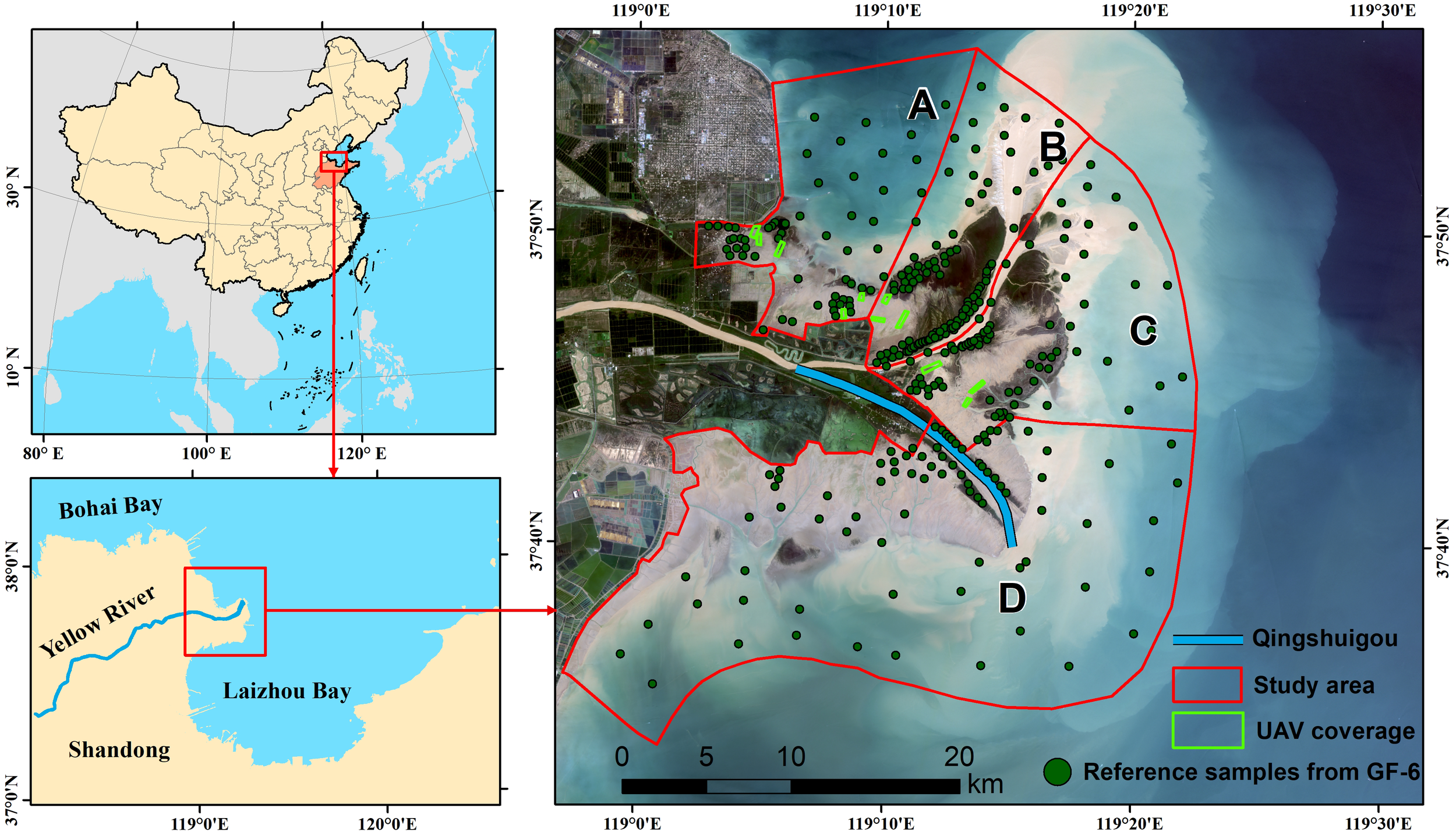
Location of the study area. Qingshuigou course was the old river channel before 1996. The study area is divided in Zone (A–D) based on the distribution of artificial groins and the river channel.
2.2 Landsat 8 imagery and pre-processing
Landsat 8 satellite is a multispectral imaging satellite launched in 2013. Its carries Operational Land Imager (OLI) sensor with 9 spectral bands from visible to shortwave infrared wavelengths. We downloaded all available Landsat 8 Level 2 Tier 1 surface reflectance images covering the study area (Row 121, Path 43) acquired during January 1, 2020 ~ December 31, 2020 from Google Earth Engine (GEE) platform. The quality assessment (QA) bands of the images were used to identify the area covered by clouds and cloud shadows. There were 18 images in total, and the average cloud coverage was 29.2%. Figure 2 illustrates the spatial distribution of the number of valid observations (no cloud/cloud shadow). The average number of valid observations is 12.7 per pixel, while the number was 11.5 per pixel over the intertidal area.
Figure 2
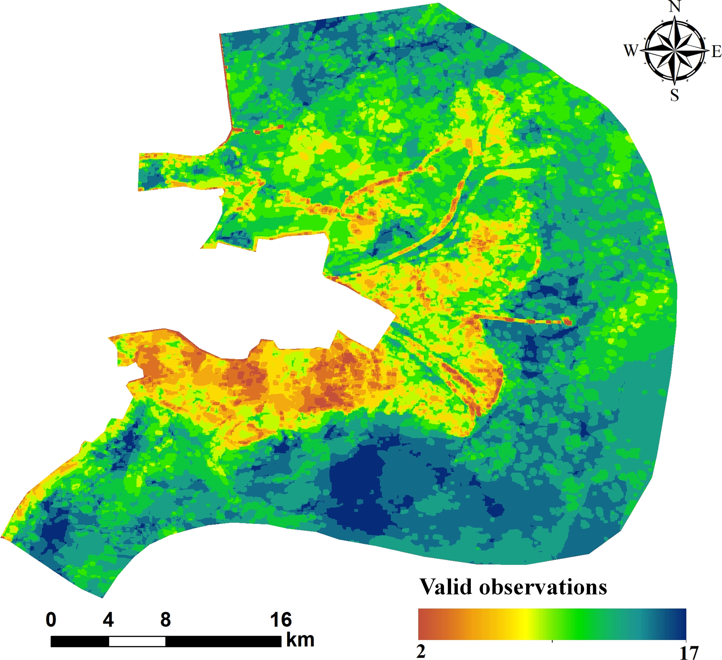
Landsat 8 OLI good observations in the Yellow River Delta in 2020.
2.3 Auxiliary data and preprocessing
Auxiliary datasets include high-spatial-resolution images taken by DJI Phantom 4 Multispectral (P4M) Unmanned Aerial Vehicle (UAV) and Gaofen-6 satellite images, which were primarily used for reference data collection. DJI P4M UAV carries a RGB camera and a multispectral sensor with 5 spectral bands including blue, green, red, red-edge and near-infrared (NIR). In September 2020, around 11 UAV flights with an average coverage of 10.2ha were taken in the study area (Figure 1). For each flight, the flight height was 50 m, resulting in 2.65 cm spatial resolution. The along path and cross path overlapping area were over 70%. Within the coverages of UAV flights, 68 field plots with size 1m × 1m were randomly selected. Location of each plot was recorded with handheld GPS RTK equipment, the vegetation species, density and growth status were also recorded at the field surveys. For all UAV images, DJI Terra software was used to generate multispectral orthophoto images. The ortho-images were then segmented into objects using multiresolution segmentation algorithm embedded in eCognition software. Base on the vegetation indexes calculated for each object, the threshold method was used to classify the objects into bare flat, S. salsa, S. alterniflora and P. australis. The classification maps were then upscaled to Landsat 30 m resolution and the fractional cover of each vegetation type within 30 m-grids were calculated using area aggregation approach. The total of 112.3 ha UAV flight coverage resulted in 826 samples.
Because many areas in the YRD wetlands were difficult to access, the UAV flight coverages and the reference samples generated from the UAV images were limited. To supplement the reference samples, high-spatial resolution imagery acquired by Gaofen 6 satellite (GF-6) on September 4, 2020 was used to generate additional reference samples of fractional cover. GF-6 is a high-spatial-resolution satellite that was launched in 2018 as one of the series of China High-resolution Earth Observation System (CHEOS) satellites. It carries a 2-meter resolution panchromatic camera and an 8-meter multi-spectral imager with blue, green, red, and near-infrared band. We first fused the panchromatic imagery with the multispectral imagery using NNDiffuse Pan Sharpening method to obtain 2 meters-resolution multispectral image. Then, we utilized the dimidiate pixel model to estimate the fractional vegetation cover for every 2 m pixel (Song et al., 2022). As the dimidiate pixel model cannot discriminate vegetation species, we only selected those pixels that contain a single vegetation species as reference pixels. Expert knowledge and field experiences helped to determine whether a pixel contain one species. For example, S. alterniflora at the landward edge is unlikely mixed with other species (Zhang et al., 2020). As a result, 348 sample points were generated based on GF-6 images (Figure 1).
3 Methods
In this study, we developed a machine learning-based ensemble model for fractional cover estimation for different salt marsh vegetation species based on time series Landsat imagery (Figure 3). The ELM aimed to enhance the performance of each individual model and improve the fractional cover estimation accuracy. Temporal composite spectral features were generated from time series Landsat imagery. As some Landsat images have cloud and cloud shadow contamination, we conducted cloud removal with the newly proposed VICR algorithm. In order to compare and verify the role of cloud removal in vegetation coverage estimation, we compared the fractional cover estimation accuracies by using the original time-series Landsat images and the cloud-removed images. Section 3.1 and Section 3.2 briefly introduces the VICR cloud removal algorithm and generation of temporal features, respectively. Section 3.3 describes the details of the ELM; Section 3.4 describes the accuracy assessment approach and the scenarios tested in our study.
Figure 3
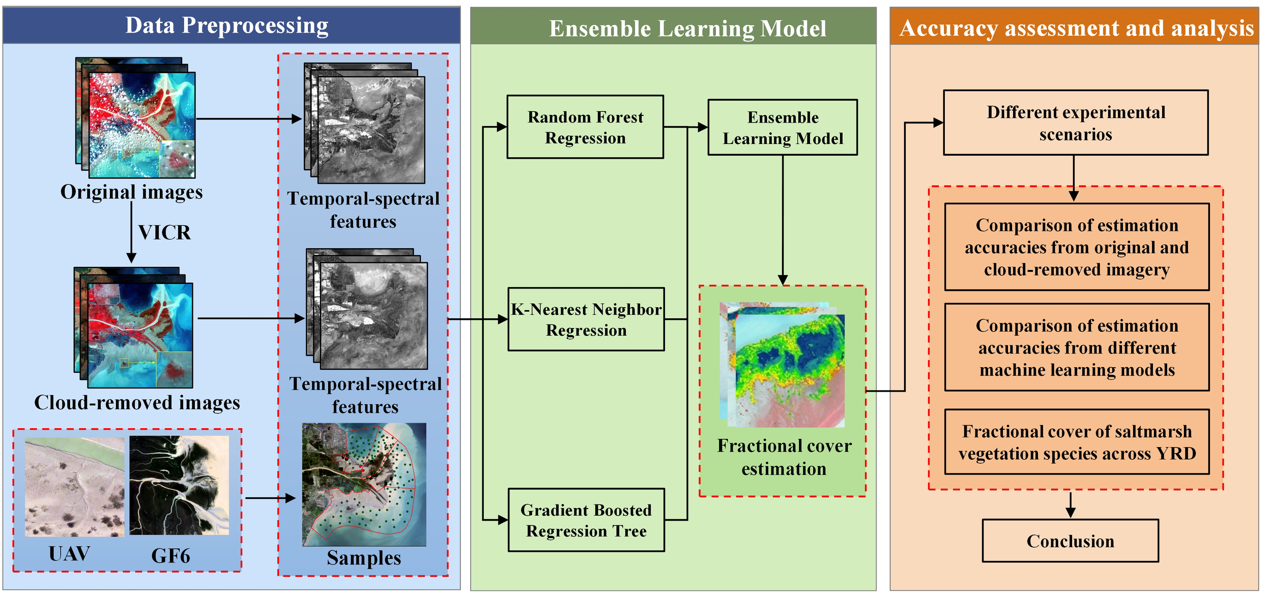
Flowchart of the study.
3.1 Cloud removal for Landsat imagery using VICR algorithm
To date, many cloud removal algorithms have been developed (Zhu et al., 2012a; Cao et al., 2020; Wang et al., 2022). These algorithms used one or more cloud-free imagery as reference images to predict the missing values in the cloud and cloud shadows in the target image (i.e., the cloud image). However, these algorithms had limited performance when dealing with landscapes with abrupt changes (Wang et al., 2022) such as the estuarian wetlands that are frequently inundated by tidal water.
To solve the above problems, our previous research proposed VICR, a new cloud removal algorithm based on time series reference images. VICR implements cloud removal by filling each cloud region separately. For each cloud region, it consists of three steps: (1) Virtual image construction by linear transformation using time series Landsat imagery. In this step, optimal number of reference images is determined. (2) Similar neighboring pixel selection with assist of a newly proposed temporal-weighted spectral distance. (3) Residual image estimation and cloud image reconstruction by adding residual image to the virtual image. VICR also proposed a strategy for time-series cloud image processing. Details of the model can be found in Wang et al. (2022). Following this strategy, the Landsat imagery acquired in 2020 over the study area (Table 1) were sorted in the order of the cloud cover percentage; the image with the lowest cloud cover was processed first and then the cloud-removed image was used as reference image for images with larger cloud cover.
Table 1
| Date | Cloud cover (%) | Date | Cloud cover (%) |
|---|---|---|---|
| Jan-10 | 21 | Jul-20 | 1.4 |
| Feb-11 | 82.8 | Aug-21 | 38.2 |
| Mar-14 | 0.2 | Sep-06 | 27 |
| Mar-30 | 0 | Sep-22 | 64.2 |
| Apr-15 | 40 | Oct-08 | 72.5 |
| May-01 | 0.4 | Oct-24 | 0.4 |
| May-17 | 0.8 | Nov-25 | 34.9 |
| Jun-02 | 51.4 | Dec-11 | 16.3 |
| Jul-04 | 53.3 | Dec-27 | 21.7 |
Landsat 8 OLI images acquired in 2020 over the study area.
3.2 Generation of temporal features
Temporal information is helpful to distinguish different salt marsh vegetation types and different fractional cover of the same vegetation type (Song et al., 2022). Our previous research found that temporal composite of spectral indices as input features help to discriminate different coastal wetland cover types (Wang et al., 2021b). We also found that the harmonic regression features improved the classification accuracies. Harmonic regression fits the time series spectral indices [such as the normalized difference vegetation index (NDVI)] using superposition of periodic curves and can well represent the phenological pattern of each vegetation species. Following our previous study, we first calculated seven spectral indexes from each Landsat 8 OLI images in 2020 (Wang et al., 2021b), including Normalized Difference Vegetation Index (NDVI), Enhanced Vegetation Index (EVI), Soil Adjustment Vegetation Index (SAVI), Green Chlorophyll Vegetation Index (GCVI), Green Normalized Difference Vegetation index (GNDVI), Land Surface Water Index (LSWI) and Modified Normalized Difference Water Index (MNDWI). NDVI is the most common vegetation index to reflect the vegetation type and growth status (Tucker, 1979). EVI takes into account the canopy background and aerosol influences, so it is more sensitive to high biomass than NDVI (Huete et al., 2002). Compared to NDVI, SAVI is more suitable for low vegetation cover areas because it adds soil adjustment coefficient (Huete, 1988). GCVI has a larger dynamic range than NDVI and is suitable for densely vegetation areas (Grevstad et al., 2003). GNDVI has significant correlation with chlorophyll content and leaf area index (Gitelson and Merzlyak, 1998). LWSI is sensitive to canopy water content and soil moisture (Xiao et al., 2005), and MNDWI is good at identifying open water (Xu, 2006). The spectral indices were calculated using the following functions:
where ρblue ρgreen, ρred, ρNIR and ρSWIR1 are the surface reflectance in blue, green, red, near infrared and short-wave infrared 1 bands in Landsat 8 OLI images.
The annual maximum, minimum, mean, median and standard deviation of the six spectral bands (blue, green, red, NIR, SWIR1 and SWIR2) and the seven spectral indexes were calculated for each pixel based on all Landsat imagery in 2020. Therefore, a total of 39 temporal composite images were generated.
In addition, the Harmonic ANalysis of Time Series (HANTS) method was used for all spectral indexes with obvious periodicity except for MNDWI. This method is beneficial to identify plant phenology, which helps to distinguish different plants (Zhou et al., 2015). The mathematical expression of HANTS used in this study is as follows:
where A is the amplitude of the harmonic wave, which represents the fluctuation range of the spectral index time series curve; the value can reflect the difference in productivity of different vegetation types in the whole cycle. Phase φ represents the peak time of spectral index, i.e., the peak time of vegetation growth. a0 is the remainder value of the curve, representing the annual average value of the spectral index. In this study, the amplitude, phase and remainder of six spectral indexes constituted a total of 18 harmonic regression features.
3.3 Ensemble learning model
The ELM combined Random Forest Regression (RFR), K-Nearest Neighbor Regression (KNNR) and Gradient Boosted Regression Tree (GBRT). RFR is composed of multiple regression trees based on the bagging algorithm. There is no association with each decision tree in the forest, and the final output of the model is jointly determined by each decision tree. The selection of samples and features in RFR is random, which can effectively reduce the occurrence of over fitting. In addition, RFR can evaluate the importance of different features, has strong processing ability for high-dimensional data, and has a certain anti-noise ability, which makes this method widely used in remote sensing data (Ge et al., 2020; Yang et al., 2020). KNNR is an instance-based machine learning regression model which assumes that similar samples are more proximity in the feature space (Ge et al., 2020). In the process of regression prediction, the value of k neighbors is used as the prediction result. KNNR needs to normalize all features first, and then choose a distance measurement method to calculate the similarity between pixels. In this paper, Euclidean distance was used to calculate the similarity. GBRT is also a regression-tree-based machine learning model. Different from RFR where each regression tree is independent, GBRT connects each tree (weak learner) in a linear combination to continuously reduce the residual errors by the loss function. (Di et al., 2019; Yu et al., 2021). In the training process of GBRT, weak learners are generated through multiple iterations, and each learner is trained according to the residuals of the previous learner. Through iterative improvement of each weak learner, the GBRT model is finally obtained.
The ELM developed in this study integrated three models by using GBRT model. This is because that GBRT model has the following advantages: (1) strong prediction ability for low dimensional data; (2) strong processing ability for nonlinear data; and (3) strong flexibility in handling various continuous values, discrete values, and other types of data. Specifically, the predicted values from each of the RFR, KNNR and GBRT were used as temporal-spectral features, and the same training samples for each individual model were used to train the GBRT model, which was then used to predict the fractional cover of salt marsh vegetation species. Different machine learning models all used the grid search method to determine the optimal parameters.
3.4 Experimental scenarios and accuracy assessments
We aimed to investigate whether the cloud-removed imagery help to enhance the fractional cover estimation of different salt marsh species, and whether the ensemble learning regression algorithm helped to improve the accuracies. For this purpose, we designed four experimental scenarios as follows.
-
Scenario 1: All 57 temporal features (temporal composite features and harmonic regression features) were generated based on the original Landsat imagery (cloud and cloud shadows were masked out) and the cloud-removed Landsat imagery, respectively; Using these temporal features as input features, the ensemble learning regression model, as well as each individual model was used as fractional cover estimation model.
-
Scenario 2: A total of 39 composite features (i.e., the harmonic regression features were removed) were generated based on the original Landsat imagery (cloud and cloud shadows were masked out) and the cloud-removed Landsat imagery, respectively; Using these temporal features as input features, the ensemble learning regression model, as well as each individual model was used as fractional cover estimation model.
-
Scenario 3: same as Scenario 1 unless that Landsat images acquired in March, July and October were eliminated from the original image sets.
-
Scenario 4: same as Scenario 2 unless that Landsat images acquired in March, July and October were eliminated from the original image sets.
For each scenario, we can compare the estimation accuracies from the original imagery with those from the cloud-removed imagery; we can also compare the accuracies from each of the individual models and that from the ELM. By comparing scenario 1 with scenario 3 and by comparing scenario 2 with scenario 4, we can evaluate whether cloud removal can compensate the unavailability of observations during critical months. By comparing scenario 1 with scenario 2 and by comparing scenario 3 with scenario 4, we can evaluate the role of harmonic regression. Note that harmonic regression is essentially a gap filling algorithm which can build full time series observations, although its purpose is not recovering missing values obscured by cloud/cloud shadow.
For each scenario, ten-fold cross validation was used to evaluate the model performance. Specifically, the model was trained for ten times, at each time the model is fitted by a training data set consisting of randomly selected 90% of the total reference data, and the remaining 10% was used for validation. The accuracy assessment metrics include determination coefficient (R-square), Root Mean Square Error (RMSE) and Mean Absolute Error (MAE), and the formula are as follows:
where yi represents the reference fractional cover measured by UAV or high-spatial-resolution imagery, represents the mean value of reference fractional cover, and represents the predicted fractional cover. R-square represents the reliability of the regression model. Larger R-square indicates higher fitting accuracy. MAE can measure the average absolute difference between the fractional cover estimation and the reference values. RMSE is similar to MAE, but it can amplify larger errors.
4 Results
4.1 Comparison of fractional cover estimation accuracies from original and cloud-removed imagery
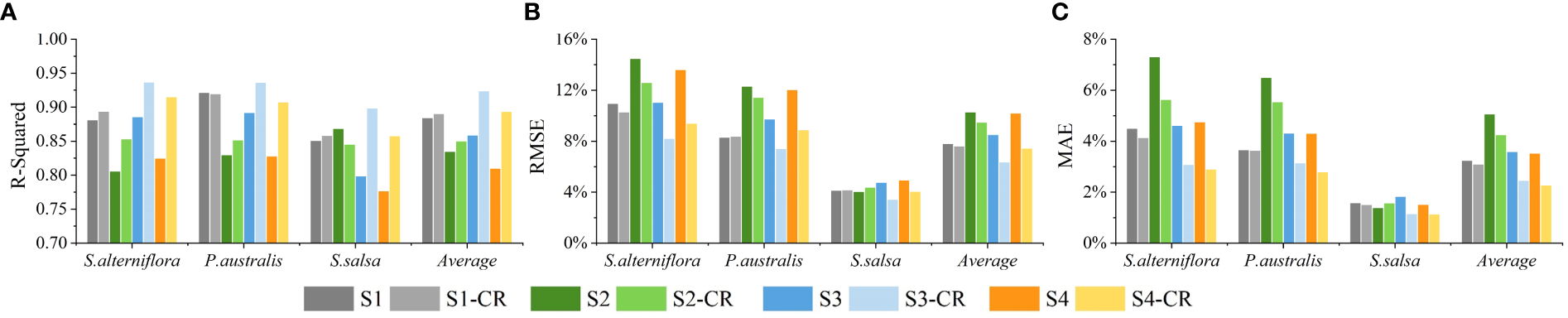
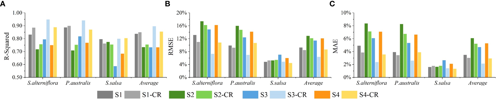
Figures 4 –7 showed the fractional cover estimation accuracies of the four scenarios using RFR, KNNR, GBRT and ELM, respectively. For all three vegetation species, the fractional cover estimation accuracies using the cloud-removed imagery were higher (greater R-square, lower RMSE and MAE) than those using the original imagery regardless of the scenarios and the machine learning models (expect for S.salsa in Scenario 2). Although the fractional cover estimation accuracies were different, all three independent models showed similar patterns as the ELM. The improvements were especially noticeable in Scenario 3 and Scenario 4 when assuming the images in March, July and October were unavailable. For example, for ELM, in Scenario 3 the average R-square increased from 0.859 to 0.922 (RMSE decreased from 8.4% to 6.2%), and in Scenario 4 the average R-square increased from 0.818 to 0.902 (RMSE decreased from 10.1% to 7.2%) when cloud removal was performed (Figure 7). However, when all the original Landsat images were used, good accuracies could be achieved even without cloud removal as long as harmonic regression parameters were added as input features, and the improvement resulted from cloud removal was minimal. For example, for ELM, in Scenario 1 the average R-square was 0.881 when the original Landsat images were used, and the average R-square was 0.891 when all cloud-removed imagery were used (Figure 7A). When the harmonic regression parameters were not involved in the fractional cover estimation model (Scenario 2), the accuracies considerably decreased, with R-square of only 0.839 with the original imagery and 0.849 with the cloud-removed imagery. This indicates that the harmonic regression features were more important than removing clouds from the images in discriminating saltmarsh species as well as in discriminating the vegetation cover differences if the time series images were sufficient. When the images in March, July and October were not involved, the fractional cover estimation accuracies decreased significantly even when the harmonic regression features were used, especially for S.salsa and the average accuracies (Scenario 3 vs. Scenario 1 without cloud removal). For the ELM, the R-square of the estimated S.salsa fractional cover declined from 0.854 to 0.794 when images acquired during the three months were not used. In this case, cloud removal for the remaining images improved the accuracies substantially. And the R-square of the estimated S. salsa fractional cover was 0.889 (S3-CR in Figure 7), even higher than Scenario 1 (S1-CR in Figure 7A). In general, cloud removal is helpful to improve the accuracy of fractional cover estimation, especially when there are few good observations.
Figure 4
(A) R-square, (B) RMSE and (C) MAE of the fractional cover estimation of different salt marsh vegetation species from four scenarios using Random Forest Regression model. S1~S4: Scenario 1 ~ Scenario 4 based on the original Landsat imagery; S1-CR ~ S4-CR: Scenario 1 ~ Scenario 4 based on the cloud-removed Landsat imagery.
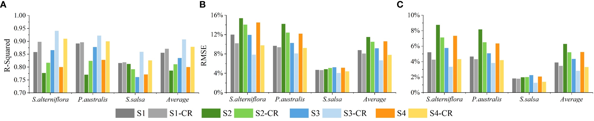
Figure 5
(A) R-square, (B) RMSE and (C) MAE of the fractional cover estimation of different salt marsh vegetation species from four scenarios using K-Nearest Neighbor Regression model. S1~S4: Scenario 1 ~ Scenario 4 based on the original Landsat imagery; S1-CR ~ S4-CR: Scenario 1 ~ Scenario 4 based on the cloud-removed Landsat imagery.
Figure 6
(A) R-square, (B) RMSE and (C) MAE of the fractional cover estimation of different salt marsh vegetation species from four scenarios using Gradient Boosting Regression Tree model. S1~S4: Scenario 1 ~ Scenario 4 based on the original Landsat imagery; S1-CR ~ S4-CR: Scenario 1 ~ Scenario 4 based on the cloud-removed Landsat imagery.
Figure 7
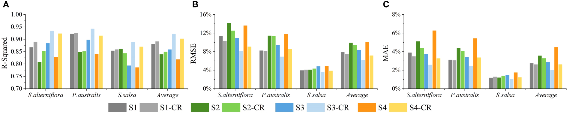
(A) R-square, (B) RMSE and (C) MAE of the fractional cover estimation of different salt marsh vegetation species from four scenarios using Ensemble Learning model. S1~S4: Scenario 1 ~ Scenario 4 based on the original Landsat imagery; S1-CR ~ S4-CR: Scenario 1 ~ Scenario 4 based on the cloud-removed Landsat imagery.
4.2 Comparison of fractional cover estimation accuracies from different machine learning models
From Figures 4-7, the ELM generally achieved the best accuracies for all scenarios regardless of using the original imagery or using the cloud-removed imagery. Tables 2–4 respectively list the R-squares, RMSEs and MAEs of the estimated fractional cover derived from RFR, KNNR, GBRT and the ELM in Scenario 1 based on the cloud-removed images. The average R-square of the ELM estimation was 0.891, the average RMSE was 7.5% and the average MAE was 2.6%, which was higher than each individual model. Among the three individual models, RFR yielded the highest accuracies, slightly lower than those of the ELM. Compared to KNNR and GBRT, the accuracy was significantly improved when the models were integrated through GBRT, indicating that the GBRT can learn the residuals of each individual model through the integration process and effectively improve the estimation accuracy. For example, the average RMSE of the three-sub models is 8.03%, while the RMSE of the ELM is 7.48% (Table 4). Especially for P.australis, the RMSE of the three sub-models is 2.87%, while the RMSE of the ELM is 8.96%, and the RMSE decreases by an average of 9.97%, which indicating that ELM significantly improved the estimation accuracy of fractional cover of P.australis. Table 2 showed the accuracy of vegetation coverage estimation of P.australis is the highest, followed by S.alterniflora, and finally S.salsa. The average R-square values of their sub-models are 0.905, 0.891, and 0.812 respectively. And for the ELM, the R-square for P.australis, S.alterniflora and S.salsa were 0.924, 0.890 and 0.859 respectively. For S. alterniflora, although the R-square of the ELM was very close to the average R-square of the three models, the ELM has obvious improvement in MAE. This also shows that the integration process can help improve the estimation accuracy.
Table 2
| RFR | KNNR | GBRT | Average of the three models | ELM | |
|---|---|---|---|---|---|
| P.australis | 0.919 | 0.899 | 0.896 | 0.905 | 0.924 |
| S.salsa | 0.857 | 0.762 | 0.818 | 0.812 | 0.859 |
| S.alterniflora | 0.893 | 0.884 | 0.897 | 0.891 | 0.890 |
| Average | 0.889 | 0.849 | 0.870 | 0.869 | 0.891 |
R-square of the estimated fractional cover based on cloud-removed images in Scenario 1.
RFR, Random Forest Regression; KNNR, K-Nearest Neighbor Regression; GBRT, Gradient Boosted Regression Tree; ELM, Ensemble Learning Model.
Table 3
| RFR | KNNR | GBRT | Average of the three models | ELM | |
|---|---|---|---|---|---|
| P.australis | 3.62 | 3.44 | 4.31 | 3.79 | 3.06 |
| S.salsa | 1.49 | 1.78 | 1.8 | 1.69 | 1.3 |
| S.alterniflora | 4.12 | 3.85 | 4.25 | 4.07 | 3.48 |
| Average | 3.08 | 3.02 | 3.45 | 3.18 | 2.61 |
MAE (%) of the estimated fractional cover based on cloud-removed images in Scenario 1.
RFR, Random Forest Regression; KNNR, K-Nearest Neighbor Regression; GBRT, Gradient Boosted Regression Tree; ELM, Ensemble Learning Model.
Table 4
| RFR | KNNR | GBRT | Average of the three models | ELM | |
|---|---|---|---|---|---|
| P.australis | 8.34 | 9.16 | 9.39 | 8.96 | 8.07 |
| S.salsa | 4.13 | 5.28 | 4.63 | 4.68 | 4.09 |
| S.alterniflora | 10.27 | 10.98 | 10.18 | 10.48 | 10.28 |
| Average | 7.58 | 8.47 | 8.06 | 8.04 | 7.48 |
RMSE (%) of the estimated fractional cover based on cloud-removed images in Scenario 1. RFR, Random Forest Regression; KNNR, K-Nearest Neighbor Regression; GBRT, Gradient Boosted Regression Tree; ELM, Ensemble Learning Model.
Figure 8 presents the fractional cover maps of the three salt marsh vegetation types estimated by each individual model and ELM respectively. All four models show generally similar spatial patterns of dense patches of S.alterniflora and P.australis: dense coverage (fractional cover over 0.5) of S.alterniflora was mainly distributed near the river mouth, while dense coverage of P.autralis was distributed along the river bank. However, considerable differences existed in terms of the distributions of low coverage of different vegetation types. From the KNNR model, low density S. alterniflora (fractional cover between 0.1 and 0.4) was widely distributed in the supra tidal zone (Zone D), where S. alterniflora growth is impossible due to high frequency of inundation. Compared to the GBRT model, wide area of P.australis with low density was distributed in the supratidal zone in Zone D, which was also inconsistent with the reality. In addition, a small patch of high-density P.australis (fractional cover over 0.8) was found through GBRT model in the sand bar at the river mouth (Zone C), which is also unlikely to occur. In contrast, the spatial extent estimated by RFR and GBRT was similar, but there were considerable differences in the fractional cover estimations for each vegetation type. For example, the spatial extent of S.alterniflora estimated by RFR model is much smaller than that estimated by GBRT in the south coast. But it is obvious that S.alterniflora should not grow on the sea, and there are some errors in both models. On the tidal flat of the south bank, the spatial extent of P.australis estimated by RFR model is less than that estimated by GBRT, while the estimations for S.salsa by two models are obviously opposite.
Figure 8
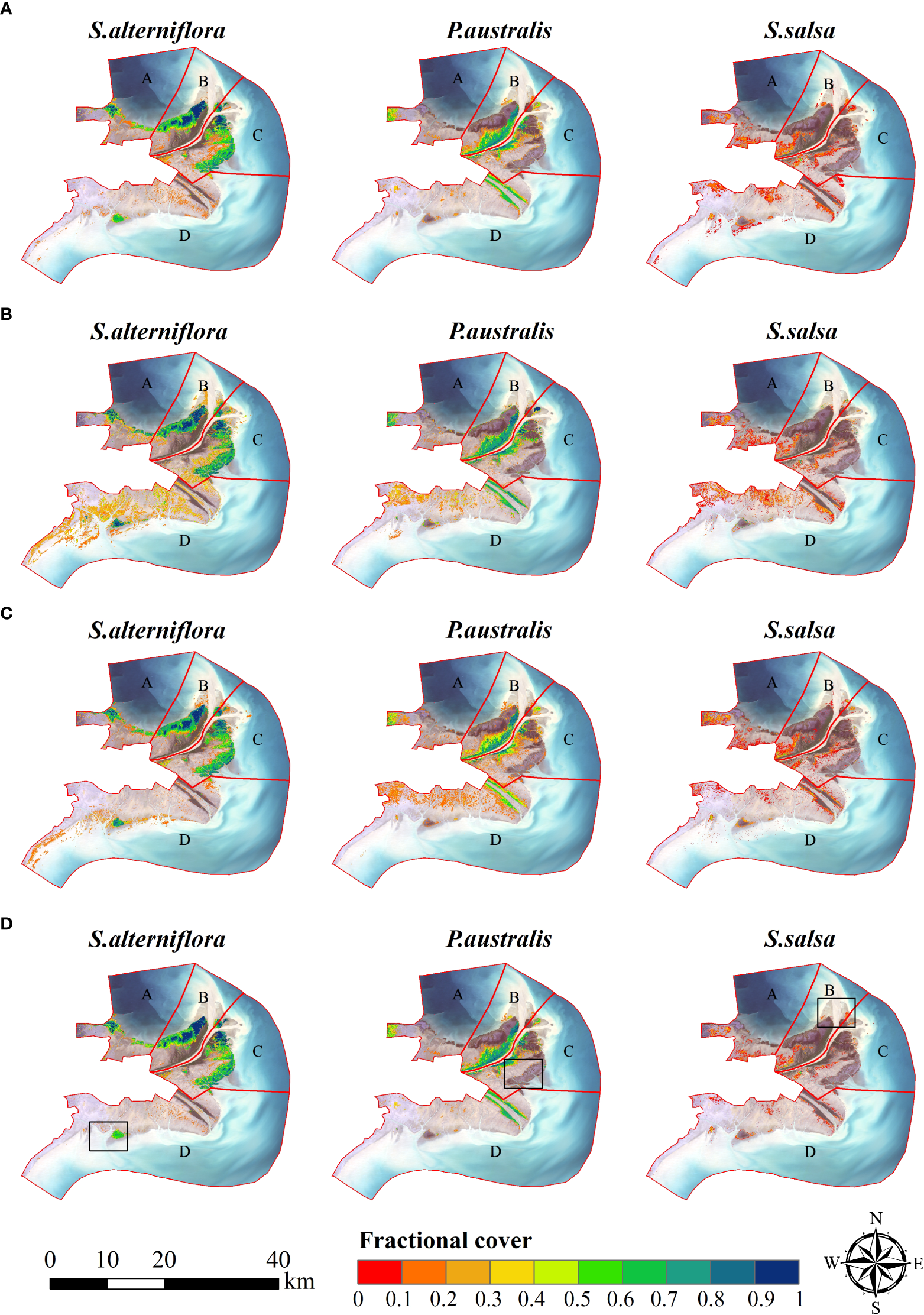
The fractional cover of three salt marsh vegetation species based on different machine learning model. (A) based on RFR; (B) based on KNNR; (C) based on GBRT and (D) based on ELM.
Although there are some obvious errors in the fractional cover estimated by each individual models, the estimation accuracy was significantly improved by integrating the estimation results with the GBRT. For example, the over-estimation of S.alterniflora coverage along the south coast was significantly reduced, and the newly formed S.alterniflora patches can still be discovered. The estimated fractional cover of P.australis was also more reasonable. In the middle-low intertidal area with high soil salinity, the over-estimation of P.australis coverage is significantly reduced. Compared to the other two vegetation types, the final estimated fractional cover of S.salsa was low (ranging from 0.05 to 0.3) and the spatial extents of S.salsa was smaller than that estimated from the other models, which was consistent with field investigations and our previous reports (Han et al., 2022b). S.salsa is vulnerable to the tidal influence and the plants are generally sparse, therefore the estimation for S.salsa coverage is relatively difficult. By combining the three models, the fractional cover estimation for S.salsa was more robust. In general, the integration of the three individual models helps to improve the fractional cover estimation accuracy, and the spatial distribution of the estimated fractional cover of the saltmarsh vegetation species by the ELM is more reasonable.
4.3 Fractional cover of saltmarsh vegetation species across YRD
The results from ELM showed that the three species, S. alterniflora, P. australis and S. salsa, covered 5753.97 ha, 4208.4 ha and 1984.41 ha, respectively; and the average fractional cover was 58.45%, 51.64% and 51.64%, respectively. The fractional vegetation cover maps (Figure 8D) showed that P.australis was mainly distributed along the river banks and along the Qingshuigou course, the old river channel before 1996 (Figure 1). According to the zonal statistics (Figure 9A), the average fractional cover of P.australis was the highest in Zone B, which is 58.26%. The average fractional cover of P.australis in Zone D and in Zone C were 48.93% and 48.47%, respectively. Zone C demonstrated large spatial variation in P.australis coverage (Figure 9A). The coverage showed decreasing trend from the river banks to the tidal flats. This is consistent with the existing field-based studies (Xie et al., 2021), which reported that the biomass and coverage of P.australis decreased with increasing soil salinity and decreasing freshwater supply in the tidal flat. The coverage along the old Qingshuigou course is lower than that along the current river course, which is probably due to the insufficient water supply (Wu, 2022). With the expansion of S.alterniflora, the habitat of P.australis was invaded. As a result, the spatial extent area of P.australis was much lower than that of S.alterniflora in Zone C (1152.2 ha vs. 2604.6 ha, Figure 9E). In Zone D, the area of P.australis was significantly larger than that of S.alterniflora (948.1 ha vs. 664.5 ha).
Figure 9
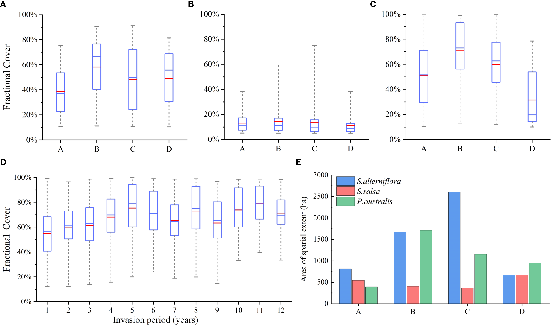
Zonal statistics of salt marsh vegetation. Box and whiskers plots of the fractional cover of (A)P.australis, (B)S.salsa, (C)S.alterniflora within different zones. (D) The box and whiskers plots of the fractional cover of S.alterniflora with different invasion years. And (E) The spatial extent area of different salt marsh vegetations within different zones. The whiskers boundaries are 25th and 75th percentile, and the blue and red lines represent the median and mean values, respectively.
S.salsa had the smallest spatial extent and lowest fractional cover among the three vegetation types (Figures 9B, E). S.salsa was mainly distributed in the mid-high intertidal area, and the average fractional cover was around 12.6%. The dams and groins in Zone A and D blocked the tide waves (Xie et al., 2018), which affected the salinity and moisture content of the intertidal zone. Figures 9E shows the average coverages of S.salsa in zone A and D (13.07% and 10.91%, respectively) were slightly lower than those in zone B and C (14.27% and 13.44%, respectively). In the west part of Zone A, S.salsa was mixed with S.alterniflora, in the landward front of S. alterniflora invasion. In Zone B and Zone C, S. salsa was mixed with P.australis around the river banks.
S.alterniflora generally has the widest spatial extent and densest fractional cover among the three vegetation types. The average fractional cover of S. alterniflora is higher in Zone B and Zone C near the river mouth than those in other zones (Figure 9C). Although the area of S.alterniflora in zone C is larger than that in zone B (2604.6 ha vs. 1672.5 ha, Figure 9E), the average fractional cover of zone B is higher (59.72% in Zone C vs. 70.82% in Zone B). S.alterniflora is also widely distributed along the coast of zone A, and the fractional cover in its west is higher than that in its east, which is associated with less tidal inundation due to higher elevation in Zone A. On the whole, the zonal difference of S.alterniflora coverage is associated with the invasion ages. S.alterniflora was first found in Zone B in 2008, then expanded to Zone A and Zone C, and finally expanded to Zone D in 2017 (Wang et al., 2021b). In addition, it has been reported that the live stem density of S.alterniflora is related to the invasion ages (Han et al., 2022a). Therefore, we calculated the statistics of fractional cover of S.alterniflora with different invasion ages (Figure 9D). Figure 9D shows that the coverage of S.alterniflora gradually increased during the first five years of the invasion (average values from 55.04% with 1 year of invasion to 75.42% with 5 years of invasion), and then kept high (around 70%). It is worth mentioning that in other studies (Wang et al., 2021b; Han et al., 2022a), they are also reported that the first five years of invasion is the key period for the expansion of S.alterniflora.
5 Discussion
5.1 Necessities of cloud removal in fractional cover estimation for saltmarsh species
Cloud contamination is inevitable in optical remote sensing, especially for the optical imagery acquired over the cloudy coastal area. To date, many algorithms, such as mNSPI, GNSPI, WLR, ARCC, have been developed for removing clouds/cloud shadows and reconstructing missing images (Zhu et al., 2012a; Zhu et al., 2012b; Zeng et al., 2013; Cao et al., 2020). Compared to the number of algorithms that have been developed, the number of applications are limited. A few studies in recent years have applied cloud removal as preprocessing step for phenological metrics derivation (Tian et al., 2020; Zhu et al., 2021), paddy rice mapping (Zhao et al., 2021) or vegetation cover estimation (Wang et al., 2020). Zhu et al. (2021) built time-series cloud-free Landsat imagery by reconstructing cloud-contaminated imagery using NSPI algorithm and then derived dry-season phenology in tropical forest. Their study found that cloud removal could help better characterize the phenological features. Zhao et al. (2021) applied mNSPI to remove cloud from Landsat imagery, and then extracted phenological features from the time series imagery for paddy rice mapping. They mentioned that the mNSPI could not accurately restore the small and continuous boundaries on the image under the clouds. Wang et al. (2020a) is probably the only study that applied cloud removal algorithm (GNSPI algorithm) to build cloud-free Landsat imagery for green vegetation cover estimation. However, their study did not estimate vegetation cover at species level.
Most of the existing studies applied the cloud removal for constructing time-series imagery, based on which phenological features can be derived. However, cloud removal may not be the necessary step for phenological features retrieval, although few studies have discussed this issue. Time-series vegetation indices can also be reconstructed by fitting and filtering methods, such as harmonic regression (Yan and Roy, 2020) or Savitzky-Golay filtering method (Chen et al., 2021). For example, the harmonic regression utilized in our study produced a simplified continuous time-series curve that can fill the data gaps. Interestingly, our results showed that cloud removal is not necessary in all cases. When the number of Landsat imagery were sufficient and temporal features based on harmonic regression were used, cloud removal did not significantly improve the fractional cover estimation accuracy (Scenario 1) (Figures 4A–C). In this case, it seemed that harmonic regression played more important roles than cloud removal in fractional cover estimation, as the accuracies decreased significantly without the temporal features derived by harmonic regression. However, when the Landsat observations during the critical months were not incorporated, cloud removal for the remained imagery was very important (Scenario 3), while harmonic regression did not help to improve the accuracy. Different from green vegetation cover estimation, the fractional cover estimation at species level not only needs to build the relationship between the temporal features and the fractional cover, but also needs to discriminate among the species. Our previous research showed that the imagery in the key months was critical to represent the phenological patterns of each species and to ensure the discrimination accuracy (Wang et al., 2021b). P. autstralis starts to grow in April, reaches the maximum greenness during July and August, and enters senescence in September. S.alterniflora starts to grow in late May and early June, reaches the maximum greenness during August and September, and then enters senescence in late October to early November (Han et al., 2022a). S. salsa presents red-purple color and the abundance reached the maximum during October. When the images during the critical months are absent, harmonic regression cannot represent the correct phenological patterns. In this case, the remaining cloud-removed images provides important supplementary information. Surprisingly, we found that the utilization of all available cloud-removed imagery produced even slightly lower accuracies than that excluding the critical months. Detailed examination showed that the reconstructed imagery in October had poor visual effects because the cloud covered almost the entire the saltmarsh extent in the estuary (Figure S1), which is quite challenging for all cloud-removal algorithms. This also indicates that when applying cloud removal as preprocessing step, cloud coverage and cloud-removal accuracies need to be considered.
5.2 Advantages of ELM in fractional cover estimation for saltmarsh species
Previous studies have confirmed that machine learning algorithms have great potential in green vegetation cover estimation. For example, Wang et al. (2018) reported high accuracy (RMSE=8.5%) of RFR for green vegetation cover estimation based on Sentinel-2 imagery. Yang et al. (2020) used RF soft classification method to estimate fractional abundance of halophytic species based on high-spatial resolution WorldView-2 imagery over Venice lagoon, Italy, and also achieved high accuracy (RMSE ranging from 0.06 to 0.19). However, the integration of multiple machine learning models into one ensemble model has not been introduced into vegetation cover estimation, especially at species level. Our results showed that the performance of the model can be ranked as the following order: ELM > RFR > GBRT > KNNR.
However, it was also found that the accuracy improvement of the ELM, which was measured by R-square and RMSE seemed not considerable compared to RFR. For example, the increase in the average R-square was only 0.002. Note that the accuracy assessment metrics were calculated based on reference samples, whose spatial locations might influence the evaluation. And when we looked at the spatial distribution of high to low coverage of each salt marsh species, the ELM apparently yielded more reasonable results. Some examples are shown in Figure 10, illustrating the results in zoomed-in area in Figure 8. Compared to ELM, RFR overestimated the spatial extent of S. alterniflora in the bare tidal flat close to the sea, and some S. alterniflora even appeared in the seawater (first column in Figure 10). In addition, it was unlikely that S. salsa grew on the sand bar near the river mouth (third column in Figure 10). Although both RFR and ELM over-estimated S. salsa cover in this area, ELM generally produced lower error than RFR. Previous research in other fields also reported that similar RMSEs or R-squares from different methods does not necessarily mean similar performance in every location (Di et al., 2019; Requia et al., 2020). Di et al. (2019) applied the ELM to estimation PM2.5 concentration across the contiguous United States. They found that each individual model did not perform equally well in every location or at all PM2.5 concentration levels although the overall R-squares are similar; however, the ensemble model complemented each other and produced more spatially balanced results. By integrating individual models in a non-linear manner, the model that performs better at some locations contribute more to the ensemble model, which improves the overall performance of the ELM.
Figure 10
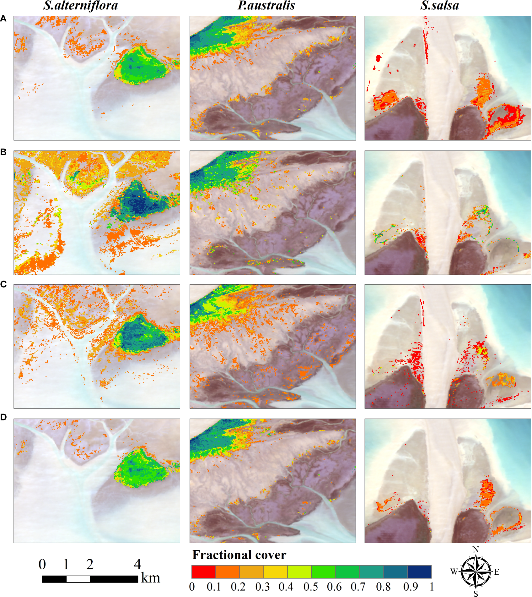
Fractional cover of S. alterniflora (left column), P.australis (middle column), and S.salsa (right column) from (A) RFR; (B) KNNR; (C) GBRT and (D) ELM in the three sub-areas shown in Figure 8D (black squares).
5.3 Uncertainties and implications for future work
The performance of the ensemble-learning-based fractional cover estimation depends on at least three factors: (1) whether the reference samples can represent the reality of fractional cover (2) whether the predictor indicators (temporal composite features used in our study) can be associated with the variability of response variable (fractional cover in our study), and (3) whether the model can capture the relationship between predictor indicators and the fractional cover of each vegetation species. Our study attempts to improve (2) and (3) by using time-series cloud-removed imagery and by developing ELM, respectively. As field surveys in coastal wetlands are difficult, in this study we relied on UAV images and GF-6 high-spatial-resolution imagery to create reference samples (Di et al., 2019; Yang et al., 2020; Song et al., 2022). Although high-spatial-resolution imagery has been widely used for reference sample collection for fractional cover estimation model, uncertainties still existed. First, the spatial coverage of each UAV flight was very small compared to the whole study area, and there might be little difference in the vegetation fractional cover over each UAV image. We need to conduct many UAV flights to generate enough reference samples, which is time and labor consuming. Second, using GF-6 and other high spatial resolution satellites would still have a certain mixed pixel effect. In the future, more efforts need to be taken to overcome the problem of sample selection. Future research will explore deep learning models for sample augmentation for the fractional cover estimation. In addition, in YRD several wetland restoration projects are being implemented in recent years. Continued monitoring of the fractional cover change in the coastal wetlands are necessary for better evaluating the effectiveness of the restoration.
6 Conclusion
In this study, we mapped the fractional cover of three major saltmarsh species, i.e., P. australis, S. salsa and S. alterniflora in the Yellow River Delta. We developed an approach framework for fractional cover estimation by utilizing the ELM based on time-series Landsat imagery which were preprocessed by VICR cloud removal. By validating with reference data collected by UAV and high-spatial-resolution GF-6 images, our results showed that the framework yielded high accuracy in fractional cover estimation, with the average R-square of 0.891, and RMSE of 7.48%.
Through experiments in four scenarios, we analyzed the role of cloud removal in fractional cover estimation and explored the advantages of ensemble model over individual models. Results showed that cloud removal as a preprocessing step can effectively improve the accuracy of vegetation coverage estimation especially when the images of key months for vegetation phenology observation (March, July and October) are missing. ELM that integrates three machine learning algorithms also helped to improve the estimation accuracy and effectively reduced the error of each individual method. The fractional cover maps revealed the spatial distribution characteristics of the three saltmarsh species, and the variations in the fractional cover are associated with invasion ages (for S. alterniflora), soil salinity and water contents. S.alterniflora covers the largest area (5753.97 ha) in the Yellow River Delta, followed by P.australis with spatial extent area of 4208.4 ha and S. salsa of 1984.41 ha. The results of this study verify the application potential of cloud removal technology and the advantages of ELM, and provide a technical framework and data support for the monitoring of native and invasive saltmarsh species in the wetlands of YRD.
Statements
Data availability statement
The original contributions presented in the study are included in the article/Supplementary Material. Further inquiries can be directed to the corresponding author.
Author contributions
ZW: Conceptualization, Data curation, Formal analysis, Investigation, Methodology, Writing – original draft, Writing – review & editing. YK: Conceptualization, Methodology, Project administration, Writing – original draft, Writing – review & editing. DL: Writing – review & editing. ZZ, QZ, YH, and PS: Investigation. ZG and DZ: Project administration. All authors contributed to the article and approved the submitted version.
Funding
This work was supported by the National Natural Science Foundation of China (No.42071396 and No.41971381) and Capacity Building for Sci-Tech Innovation—Fundamental Scientific Research Funds.
Acknowledgments
The authors are grateful for access to Landsat imagery data provided by the USGS through the Google Earth Engine cloud computation platform. The authors also thank the Yellow River Delta National Nature Reserve for their support of our work.
Conflict of interest
The authors declare that the research was conducted in the absence of any commercial or financial relationships that could be construed as a potential conflict of interest.
Publisher’s note
All claims expressed in this article are solely those of the authors and do not necessarily represent those of their affiliated organizations, or those of the publisher, the editors and the reviewers. Any product that may be evaluated in this article, or claim that may be made by its manufacturer, is not guaranteed or endorsed by the publisher.
Supplementary material
The Supplementary Material for this article can be found online at: https://www.frontiersin.org/articles/10.3389/fmars.2022.1077907/full#supplementary-material
References
1
Cao R. Chen Y. Chen J. Zhu X. Shen M. (2020). Thick cloud removal in landsat images based on autoregression of landsat time-series data. Remote Sens. Environ.249, 112001. doi: 10.1016/j.rse.2020.112001
2
Chen Y. Cao R. Chen J. Liu L. Matsushita B. (2021). A practical approach to reconstruct high-quality landsat NDVI time-series data by gap filling and the savitzky–golay filter. ISPRS J. Photogramm. Remote Sens.180, 174–190. doi: 10.1016/j.isprsjprs.2021.08.015
3
Chen B. Huang B. Chen L. Xu B. (2017). Spatially and temporally weighted regression: A novel method to produce continuous cloud-free landsat imagery. IEEE Trans. Geosci. Remote Sens.55, 27–37. doi: 10.1109/TGRS.2016.2580576
4
Chen M. Ke Y. Bai J. Li P. Lyu M. Gong Z. et al . (2020). Monitoring early stage invasion of exotic spartina alterniflora using deep-learning super-resolution techniques based on multisource high-resolution satellite imagery: A case study in the yellow river delta, China. Int. J. Appl. Earth Obs. Geoinformation92, 102180. doi: 10.1016/j.jag.2020.102180
5
Chopping M. North M. Chen J. Schaaf C. B. Blair J. B. Martonchik J. V. et al . (2012). Forest canopy cover and height from MISR in topographically complex southwestern US landscapes assessed with high quality reference data. IEEE J. Sel. Top. Appl. Earth Obs. Remote Sens.5, 44–58. doi: 10.1109/JSTARS.2012.2184270
6
Di Q. Amini H. Shi L. Kloog I. Silvern R. Kelly J. et al . (2019). An ensemble-based model of PM2.5 concentration across the contiguous united states with high spatiotemporal resolution. Environ. Int.130, 104909. doi: 10.1016/j.envint.2019.104909
7
Ding J. Na X. Li X. (2021). Wetland classification using sparse spectral unmixing algorithm and landsat 8 OLI imagery, in Spatial data and intelligence. Eds. PanG.LinH.MengX.GaoY.LiY.GuanQ.et al (Cham: Springer International Publishing), 186–194. doi: 10.1007/978-3-030-85462-1_17
8
Gao L. Wang X. Johnson B. A. Tian Q. Wang Y. Verrelst J. et al . (2020). Remote sensing algorithms for estimation of fractional vegetation cover using pure vegetation index values: A review. ISPRS J. Photogramm. Remote Sens.159, 364–377. doi: 10.1016/j.isprsjprs.2019.11.018
9
Ge G. Shi Z. Zhu Y. Yang X. Hao Y. (2020). Land use/cover classification in an arid desert-oasis mosaic landscape of China using remote sensed imagery: Performance assessment of four machine learning algorithms. Glob. Ecol. Conserv.22, e00971. doi: 10.1016/j.gecco.2020.e00971
10
Gitelson A. A. Merzlyak M. N. (1998). Remote sensing of chlorophyll concentration in higher plant leaves. Adv. Space Res.22, 689–692. doi: 10.1016/S0273-1177(97)01133-2
11
Grevstad F. S. Strong D. R. Garcia-Rossi D. Switzer R. W. Wecker M. S. (2003). Biological control of spartina alterniflora in willapa bay, Washington using the planthopper prokelisia marginata: agent specificity and early results. Biol. Control27, 32–42. doi: 10.1016/S1049-9644(02)00181-0
12
Han Y. Ke Y. Wang Z. Liang D. Zhou D. (2022b). Classification of the yellow river delta wetland landscape based on ZY1-02D hyperspectral imagery. Natl. Remote Sens. Bull. null, 1–16. doi: 10.11834/jrs.20211071
13
Han X. Wang Y. Ke Y. Liu T. Zhou D. (2022a). Phenological heterogeneities of invasive spartina alterniflora salt marshes revealed by high-spatial-resolution satellite imagery. Ecol. Indic.144, 109492. doi: 10.1016/j.ecolind.2022.109492
14
Hao J. Xu G. Luo L. Zhang Z. Yang H. Li H. (2020). Quantifying the relative contribution of natural and human factors to vegetation coverage variation in coastal wetlands in China. CATENA188, 104429. doi: 10.1016/j.catena.2019.104429
15
He J. Loboda T. V. Jenkins L. Chen D. (2019). Mapping fractional cover of major fuel type components across alaskan tundra. Remote Sens. Environ.232, 111324. doi: 10.1016/j.rse.2019.111324
16
Huete A. R. (1988). A soil-adjusted vegetation index (SAVI). Remote Sens. Environ.25, 295–309. doi: 10.1016/0034-4257(88)90106-X
17
Huete A. Didan K. Miura T. Rodriguez E. P. Gao X. Ferreira L. G. (2002). Overview of the radiometric and biophysical performance of the MODIS vegetation indices. Remote Sens. Environ.83, 195–213. doi: 10.1016/S0034-4257(02)00096-2
18
Jia K. Liang S. Gu X. Baret F. Wei X. Wang X. et al . (2016). Fractional vegetation cover estimation algorithm for Chinese GF-1 wide field view data. Remote Sens. Environ.177, 184–191. doi: 10.1016/j.rse.2016.02.019
19
Li P. Ke Y. Bai J. Zhang S. Chen M. Zhou D. (2019). Spatiotemporal dynamics of suspended particulate matter in the yellow river estuary, China during the past two decades based on time-series landsat and sentinel-2 data. Mar. pollut. Bull.149, 110518. doi: 10.1016/j.marpolbul.2019.110518
20
Mojica Vélez J. M. Barrasa García S. Espinoza Tenorio A. (2018). Policies in coastal wetlands: Key challenges. Environ. Sci. Policy88, 72–82. doi: 10.1016/j.envsci.2018.06.016
21
Mu X. Song W. Gao Z. McVicar T. R. Donohue R. J. Yan G. (2018). Fractional vegetation cover estimation by using multi-angle vegetation index. Remote Sens. Environ.216, 44–56. doi: 10.1016/j.rse.2018.06.022
22
Requia W. J. Di Q. Silvern R. Kelly J. T. Koutrakis P. Mickley L. J. et al . (2020). An ensemble learning approach for estimating high spatiotemporal resolution of ground-level ozone in the contiguous united states. Environ. Sci. Technol.54, 11037–11047. doi: 10.1021/acs.est.0c01791
23
Shanmugam P. Ahn Y.-H. Sanjeevi S. (2006). A comparison of the classification of wetland characteristics by linear spectral mixture modelling and traditional hard classifiers on multispectral remotely sensed imagery in southern India. Ecol. Model.194, 379–394. doi: 10.1016/j.ecolmodel.2005.10.033
24
Song D.-X. Wang Z. He T. Wang H. Liang S. (2022). Estimation and validation of 30 m fractional vegetation cover over China through integrated use of landsat 8 and gaofen 2 data. Sci. Remote Sens.6, 100058. doi: 10.1016/j.srs.2022.100058
25
Tian J. Zhu X. Wu J. Shen M. Chen J. (2020). Coarse-Resolution Satellite Images Overestimate Urbanization Effects on Vegetation Spring Phenology. Remote Sensing12, 117. doi: 10.3390/rs12010117
26
Tucker C. J. (1979). Red and photographic infrared linear combinations for monitoring vegetation. Remote Sens. Environ.8, 127–150. doi: 10.1016/0034-4257(79)90013-0
27
Wang B. Jia K. Liang S. Xie X. Wei X. Zhao X. et al . (2018). Assessment of sentinel-2 MSI spectral band reflectances for estimating fractional vegetation cover. Remote Sens.10, 1927. doi: 10.3390/rs10121927
28
Wang B. Jia K. Wei X. Xia M. Yao Y. Zhang X. et al . (2020a). Generating spatiotemporally consistent fractional vegetation cover at different scales using spatiotemporal fusion and multiresolution tree methods. ISPRS J. Photogramm. Remote Sens.167, 214–229. doi: 10.1016/j.isprsjprs.2020.07.006
29
Wang Z. Ke Y. Chen M. Zhou D. Zhu L. Bai J. (2021b). Mapping coastal wetlands in the yellow river delta, China during 2008–2019: impacts of valid observations, harmonic regression, and critical months. Int. J. Remote Sens.42, 7880–7906. doi: 10.1080/01431161.2021.1966852
30
Wang Z. Ke Y. Zhou D. Li X. Zhu L. Gong H. (2022) Virtual image patch-based cloud removal for landsat images. Available at: https://eartharxiv.org/repository/view/3493/ (Accessed October 20, 2022).
31
Wang X. Xiao X. Xu X. Zou Z. Chen B. Qin Y. et al . (2021a). Rebound in china’s coastal wetlands following conservation and restoration. Nat. Sustain.4, 1076–1083. doi: 10.1038/s41893-021-00793-5
32
Wang X. Xiao X. Zou Z. Hou L. Qin Y. Dong J. et al . (2020b). Mapping coastal wetlands of China using time series landsat images in 2018 and Google earth engine. ISPRS J. Photogramm. Remote Sens.163, 312–326. doi: 10.1016/j.isprsjprs.2020.03.014
33
Wu Q. (2022). Study on ecological stoichiometric characteristics in reedcommunity under different water-salt habitats in the yellow river estuary. [dissertation/master's thesis]. China: Yantai University. doi: 10.27437/d.cnki.gytdu.2022.000369
34
Wu N. Shi R. Zhuo W. Zhang C. Zhou B. Xia Z. et al . (2021). A classification of tidal flat wetland vegetation combining phenological features with Google earth engine. Remote Sens.13, 443. doi: 10.3390/rs13030443
35
Xiao X. Boles S. Liu J. Zhuang D. Frolking S. Li C. et al . (2005). Mapping paddy rice agriculture in southern China using multi-temporal MODIS images. Remote Sens. Environ.95, 480–492. doi: 10.1016/j.rse.2004.12.009
36
Xie T. Cui B. Bai J. Li S. Zhang S. (2018). Rethinking the role of edaphic condition in halophyte vegetation degradation on salt marshes due to coastal defense structure. Phys. Chem. Earth Parts ABC103, 81–90. doi: 10.1016/j.pce.2016.12.001
37
Xie X. Li X. Bai J. Zhi L. (2021). Variations of aboveground biomass of 4 kinds of typical plants with surface elevation ofWetlands in the yellow river delta. Wetl. Sci.19, 226–231. doi: 10.13248/j.cnki.wetlandsci.2021.02.010
38
Xu H. (2006). Modification of normalised difference water index (NDWI) to enhance open water features in remotely sensed imagery. Int. J. Remote Sens.27, 3025–3033. doi: 10.1080/01431160600589179
39
Xu M. Watanachaturaporn P. Varshney P. K. Arora M. K. (2005). Decision tree regression for soft classification of remote sensing data. Remote Sens. Environ.97, 322–336. doi: 10.1016/j.rse.2005.05.008
40
Yang Z. D’Alpaos A. Marani M. Silvestri S. (2020). Assessing the fractional abundance of highly mixed salt-marsh vegetation using random forest soft classification. Remote Sens.12, 3224. doi: 10.3390/rs12193224
41
Yan L. Roy D. P. (2020). Spatially and temporally complete landsat reflectance time series modelling: The fill-and-fit approach. Remote Sens. Environ.241, 111718. doi: 10.1016/j.rse.2020.111718
42
Yu R. Yao Y. Wang Q. Wan H. Xie Z. Tang W. et al . (2021). Satellite-derived estimation of grassland aboveground biomass in the three-river headwaters region of China during 1982–2018. Remote Sens.13, 2993. doi: 10.3390/rs13152993
43
Zeng C. Shen H. Zhang L. (2013). Recovering missing pixels for landsat ETM+ SLC-off imagery using multi-temporal regression analysis and a regularization method. Remote Sens. Environ.131, 182–194. doi: 10.1016/j.rse.2012.12.012
44
Zhang C. Gong Z. Qiu H. Zhang Y. Zhou D. (2021). Mapping typical salt-marsh species in the yellow river delta wetland supported by temporal-spatial-spectral multidimensional features. Sci. Total Environ.783, 147061. doi: 10.1016/j.scitotenv.2021.147061
45
Zhang X. Xiao X. Wang X. Xu X. Chen B. Wang J. et al . (2020). Quantifying expansion and removal of spartina alterniflora on chongming island, China, using time series landsat images during 1995–2018. Remote Sens. Environ.247, 111916. doi: 10.1016/j.rse.2020.111916
46
Zhao R. Li Y. Chen J. Ma M. Fan L. Lu W. (2021). Mapping a paddy rice area in a cloudy and rainy region using spatiotemporal data fusion and a phenology-based algorithm. Remote Sens.13, 4400. doi: 10.3390/rs13214400
47
Zhou J. Jia L. Menenti M. (2015). Reconstruction of global MODIS NDVI time series: Performance of harmonic ANalysis of time series (HANTS). Remote Sens. Environ.163, 217–228. doi: 10.1016/j.rse.2015.03.018
48
Zhou Z. Yang Y. Chen B. (2018). Estimating spartina alterniflora fractional vegetation cover and aboveground biomass in a coastal wetland using SPOT6 satellite and UAV data. Aquat. Bot.144, 38–45. doi: 10.1016/j.aquabot.2017.10.004
49
Zhu X. Gao F. Liu D. Chen J. (2012a). A modified neighborhood similar pixel interpolator approach for removing thick clouds in landsat images. IEEE Geosci. Remote Sens. Lett.9, 521–525. doi: 10.1109/LGRS.2011.2173290
50
Zhu X. Helmer E. H. Gwenzi D. Collin M. Fleming S. Tian J. et al . (2021). Characterization of dry-season phenology in tropical forests by reconstructing cloud-free landsat time series. Remote Sens.13, 4736. doi: 10.3390/rs13234736
51
Zhu X. Liu D. Chen J. (2012b). A new geostatistical approach for filling gaps in landsat ETM+ SLC-off images. Remote Sens. Environ.124, 49–60. doi: 10.1016/j.rse.2012.04.019
Summary
Keywords
saltmarsh, fractional vegetation cover, ensemble learning, cloud removal, spartina alterniflora , yellow River Delta (YRD)
Citation
Wang Z, Ke Y, Lu D, Zhuo Z, Zhou Q, Han Y, Sun P, Gong Z and Zhou D (2022) Estimating fractional cover of saltmarsh vegetation species in coastal wetlands in the Yellow River Delta, China using ensemble learning model. Front. Mar. Sci. 9:1077907. doi: 10.3389/fmars.2022.1077907
Received
23 October 2022
Accepted
30 November 2022
Published
21 December 2022
Volume
9 - 2022
Edited by
Chao Chen, Zhejiang Ocean University, China
Reviewed by
Laxmikant Sharma, Central University of Rajasthan, India; Ariel Blanco, University of the Philippines Diliman, Philippines; Dehua Mao, Northeast Institute of Geography and Agroecology (CAS), China
Updates
Copyright
© 2022 Wang, Ke, Lu, Zhuo, Zhou, Han, Sun, Gong and Zhou.
This is an open-access article distributed under the terms of the Creative Commons Attribution License (CC BY). The use, distribution or reproduction in other forums is permitted, provided the original author(s) and the copyright owner(s) are credited and that the original publication in this journal is cited, in accordance with accepted academic practice. No use, distribution or reproduction is permitted which does not comply with these terms.
*Correspondence: Yinghai Ke, yke@cnu.edu.cn
This article was submitted to Marine Conservation and Sustainability, a section of the journal Frontiers in Marine Science
Disclaimer
All claims expressed in this article are solely those of the authors and do not necessarily represent those of their affiliated organizations, or those of the publisher, the editors and the reviewers. Any product that may be evaluated in this article or claim that may be made by its manufacturer is not guaranteed or endorsed by the publisher.