Assessing the reliability of species distribution models in the face of climate and ecosystem regime shifts: Small pelagic fishes in the California Current System

1 Introduction

Marine fishes in many ecosystems have shifted their distribution poleward and deeper as climate change has warmed the oceans (Murawski, 1993; Perry et al., 2005; Hsieh et al., 2008; Hsieh et al., 2009; Nye et al., 2009; Pinsky et al., 2013; Poloczanska et al., 2013; Walsh et al., 2015). Many of these changes are occurring at a rate faster than in terrestrial habitats (Sunday et al., 2012; Poloczanska et al., 2013; Blowes et al., 2019; Pinsky et al., 2019). Climate velocity, a measure of the rate of temperature change across spatial gradients, has proven to be an accurate predictor of the magnitude and direction of shifts in species distributions in many ecosystems (Chen et al., 2011; Pinsky et al., 2013), although other aspects of a species’ ecological niche also influence distribution changes (McHenry et al., 2019). Throughout the 21^st century, climate models project that changes in species distribution will continue unabated or further accelerate (Cheung et al., 2009; Cheung et al., 2016b; Morley et al., 2018). Shifts in fish distribution have implications for trophic interactions (Selden et al., 2018), global biodiversity patterns (Cheung et al., 2009), and food security (Golden et al., 2016; Free et al., 2019).

Many projections of changes in fish distribution, biomass, and phenology under climate change are based on statistical models referred to as species distribution models (SDMs), ecological niche models, or bioclimate envelope models. These models link spatial and temporal variations in organismal occurrence with environmental variables (Elith and Leathwick, 2009). Based on these empirical relationships, changes in environmental conditions derived from climate models are used to project future shifts in species occurrence or abundance. Due to the growing importance of climate change, there has been a rise in studies using SDMs and aligned models over the last 20 years (Figure 1).

FIGURE 1

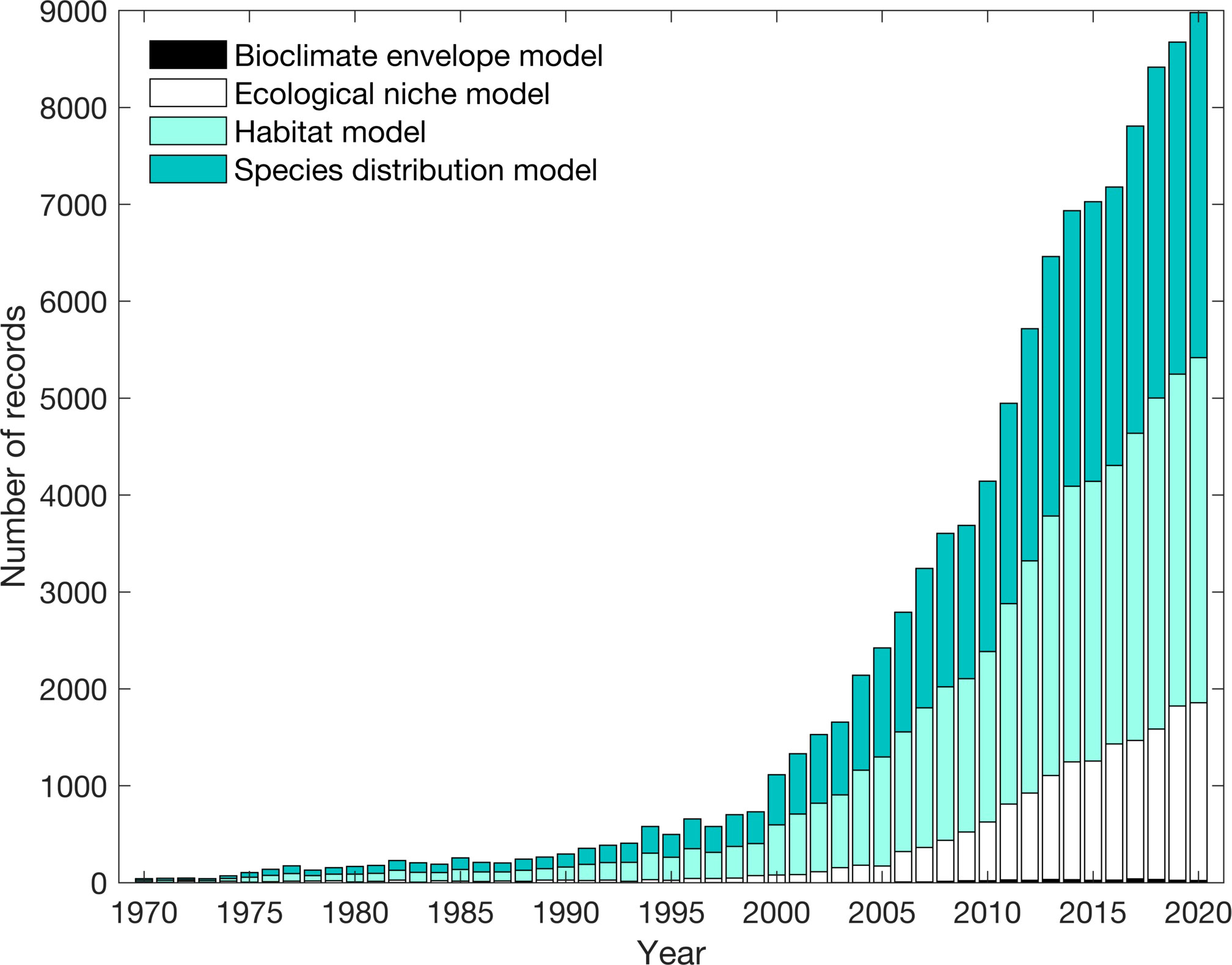
Figure 1 Web of Science search examining the cumulative number of records in the scientific literature on species distribution models, habitat models, ecological niche models, and bioclimate envelope models between 1970-2020. Five Web of Science searches were performed: (1) species AND distribution AND model*; (2) habitat AND model*; (3) ecolog* AND niche AND model*; (4) environment* AND niche AND model*, and; (5) bioclimate AND envelope AND model*. Results from the third and fourth search were combined in this figure.

A key assumption of SDMs is that the relationship between organisms and environmental conditions is stationary and not subject to changes due to variations in organismal abundance, climate, or ecosystem state. Since statistically derived relationship between a species and the environment form the basis for SDM projections, non-stationarity in this relationship could result in inaccurate projections of climate change impacts. Assumptions about stationarity in relationships between fishes and climatic variables have rarely been investigated (Litzow et al., 2019), but it is imperative to do so to assess the uncertainty associated with projections about how marine conservation initiatives will fare under climate change. Among planktonic organisms, such as dinoflagellates, diatoms, and copepods, SDMs developed using data from one decade failed to accurately project in species distribution during other decades (Brun et al., 2016). This reflects the patchy distribution of plankters, boom-bust cycles in abundance, and the potential for advection of plankton by currents outside their preferred habitat. Since projections made for copepods had greater model skill than those for primary producers, SDMs may have improved predictability for higher trophic level organisms, such as fishes. Nonetheless, recent work suggests that non-stationarity might be a common, albeit understudied, feature among SDMs that project changes in fish distribution (Litzow et al., 2018; Litzow et al., 2019; Puerta et al., 2019; Roberts et al., 2019; Litzow et al., 2020; Muhling et al., 2020).

At least seven ecological, climatic, and statistical mechanisms can lead to non-stationary fish-climate relationships. First, non-stationarity could arise if key variables influencing a species’ ecological niche are excluded from an SDM. For example, many SDMs neglect to account for interspecific relationships, such as predator-prey dynamics (Fernandes et al., 2013). Second, over-parameterization of models can lead to the appearance of non-stationarity if this results in a relationship between an environmental variable and fish distribution that is solely due to a statistical artifact. Third, non-stationarity can result from density-dependent occurrence patterns where a fish is found in its optimal habitat at low density but, as its abundance increases, spreads to additional habitats to reduce interspecific competition (MacCall, 1990). Such dynamics are especially common among small pelagic fishes (SPF)¹ (Barange et al., 2009). Fourth, overfishing can truncate fish age structure, which can increase sensitivity to climatic variables since younger and smaller fishes often exhibit heightened sensitivity (Anderson et al., 2008). Fifth, at times, fish distribution has been related to basin-scale climate indices, such as the Pacific Decadal Oscillation (PDO), North Pacific Gyre Oscillation, and North Atlantic Oscillation. Many of these indices represent statistical compilations of several climatic variables. If the relationship between these indices and local climate variables changes over time (Joyce, 2002; Litzow et al., 2018; Litzow et al., 2020), this can lead to non-stationarity between species distribution and climate indices (Litzow et al., 2018; Litzow et al., 2019; Puerta et al., 2019; Litzow et al., 2020). Also, some species have been shown to react differently to environmental conditions, such as temperature, depending on the phase of climate oscillations likely due to the influence of these oscillations on larval advection or interspecific interactions (Roberts et al., 2019). Lastly, non-stationarity across climate oscillations could occur because some climate indices, such as the PDO, are detrended. Sixth, the distribution of some species may be constrained by non-climatic factors, such as depth, reliance on biogenic habitats, or lack of dispersal corridors (Reglero et al., 2012; Asch et al., 2019). When such constraints exist, organisms may be retained in their historical habitats, even though the climate of those habitats has shifted. This can result in a non-stationary relationship between species and climate. Lastly, phenotypic plasticity, acclimation to new conditions, or rapid adaptation could lead to changes in how species distribution is related to climate (Donelson et al., 2012; Anderson et al., 2013).

Despite numerous reasons why non-stationarity may occur, there have been relatively few assessments of non-stationarity in SDMs for marine fishes due to a paucity of spatially resolved, long-term datasets that can be used to test historical changes in how fish react to the environment. One such dataset that is well suited to examine non-stationary, fish-climate relationships is California Cooperative Ocean Fisheries Investigations (CalCOFI). This program has surveyed ichthyoplankton along six transects in its core region off southern California since 1951. This region has been subject to several climate regime shifts that affected living marine resources (McGowan et al., 2003; Di Lorenzo et al., 2008; Peabody et al., 2018; Litzow et al., 2020), making it a useful testbed for evaluating whether fishes react differently to environmental variables during each phase of a regime. Also, some of the fastest rates of species distribution change in U.S. waters are projected to occur in this area (Morley et al., 2018), making it an important region for studying non-stationarity.

Our analysis of non-stationarity focuses on SPF since these species account for approximately one-third of global fish catch (Smith et al., 2011). Also, pelagic fishes are often more sensitive to climate-induced range shifts than demersal fishes (Murawski, 1993; Cheung et al., 2009; Walsh et al., 2015). SPF connect lower trophic organisms in upwelling systems with higher trophic level predators, such as piscivorous fishes, squid, seabirds, and marine mammals (Cury et al., 2011; Pikitch et al., 2014; Kaplan et al., 2017). Furthermore, their potential sensitivity to non-stationary dynamics is likely since SPF exhibit boom-bust cycles of abundance over multi-decadal periodicities (Schwartzlose et al., 1999; Chavez et al., 2003; McClatchie et al., 2017).

More specifically, we focus on four species managed under the Coastal Pelagic Species Fisheries Management Plan: northern anchovy (Engraulis mordax), Pacific sardine (Sardinops sagax), chub mackerel (Scomber japonicus), and jack mackerel (Trachurus symmetricus) [PFMC (Pacific Fishery Management Council), 2019]. Previous research has shown that these species are sensitive to fluctuations in oceanic conditions connected to climate variability and change (Lluch-Belda et al., 1991; Checkley Jr et al., 2000; Reiss et al., 2008; Rykaczewski and Checkley Jr, 2008; Weber and McClatchie, 2010; Zwolinski et al., 2011; Weber and McClatchie, 2012; Asch and Checkley Jr, 2013; Koslow et al., 2013; Howard et al., 2020).

Non-stationary relationships between SPF and environmental conditions were observed in the California Current System (CCS) in 2014-2017 when a marine heat wave (MHW) resulted in sea surface temperature (SST) anomalies exceeding three standard deviations above normal conditions (Di Lorenzo and Mantua, 2016). Historically the probability of adult S. sardinops occurrence declines when temperature exceeds 18°C, but during this event the probability of encountering S. sardinops peaked in some areas warmer than >19°C (Muhling et al., 2020). While this study did not detect similar incidents of non-stationarity when examining data from 1980 through present, it was unclear whether the rapid environmental change during the MHW was the main cause for non-stationarity or if similar non-stationary events might be observed if a longer time series were examined (Muhling et al., 2020). We addressed the latter question by determining if non-stationarity is prevalent in SDMs developed for larval E. mordax, S. sardinops, S. japonicus, and T. symmetricus between 1951-2015. This time series emphasizes the period prior to the MHW. We first determined if there were change points in time series of climate indices, oceanic variables, and fish spawning stock biomass (SSB). These change points are proxies for regime shifts. For each period associated with a different regime, we constructed a SDM for each species. Six metrics for identifying non-stationarity were inspected to determine if the relationships between fishes and oceanic conditions changed across regimes. Lastly, we examined whether SDMs developed under different regimes produce equivalent projections of future changes in fish habitat suitability under low and high greenhouse gas emissions.

2 Materials and methods

2.1 Data sources

2.1.1 Larval fish data

CalCOFI has sampled E. mordax, S. sagax, S. japonicus, and T. symmetricus larvae since 1951, with the highest concentration of samples from a core region of southern California that extends offshore from San Diego (33.0°N) to north of Point Conception (35.1°N). CalCOFI data are publicly available from the NOAA ERDDAP server.² Data on oblique ring and bongo net tows from January 1951 through April 2015 were downloaded for CalCOFI lines 76-93.3. Study sites farther offshore than CalCOFI Station 120 were filtered from this dataset because these stations were sampled less consistently. These criteria resulted in selection of 18,899 net tows. Sample collection occurred monthly during the 1950s, near monthly during the 1960s, 1970s, and early 1980s, albeit with substantial gaps during the 1970s, and quarterly since 1985. The methods for collecting and processing bongo and ring net samples were described in Kramer et al. (1972) and changes to sampling methodology were documented in Ohman and Smith (1995) and Thompson et al. (2017).

2.1.2 Oceanic data

Four environmental variables were selected for inclusion in SDMs because they were measured since 1951 concurrently at stations where CalCOFI ichthyoplankton samples were collected and because these variables were previously shown to influence target species (Checkley Jr et al., 2000; Lynn, 2003; Rykaczewski and Checkley Jr, 2008; Weber and McClatchie, 2010; Zwolinski et al., 2011; Weber and McClatchie, 2012; Asch and Checkley Jr, 2013; Weber et al., 2018; Howard et al., 2020). These variables included potential temperature, salinity, dissolved oxygen (DO), and mesozooplankton displacement volume (abbreviated as ZDV for zooplankton displacement volume). Both salinity and DO can be interpreted as indicators of water masses with distinct characteristics (e.g., Pacific subarctic water has low temperature and salinity, but high DO, whereas North Pacific Central water has high temperature and salinity, with low DO; McClatchie, 2013). Low DO can also act as a stressor affecting the physiology, distribution, and abundance of SPF (Howard et al., 2020). Upwelling of hypoxic and anoxic waters on the inner shelf has been observed in the northern CCS (Chan et al., 2008). In the southern CCS where upwelling is less vigorous, hypoxic waters do not frequently encroach into depths where SPF larvae reside (Dussin et al., 2019), so we interpret variations in DO primarily as an indicator of water mass properties. Temperature, salinity, and DO from Niskin bottles were averaged over the upper 50 m. This depth was selected because SPF eggs are most concentrated across this range (Curtis et al., 2007). Environmental data were downloaded from ERDDAP between January 1951 and February 2015 and extending between 29.7-35.3° N and 117.2-125.8° W. This area corresponded to transects selected for fish larvae. Within these constraints, 18,925 environmental observations were identified for analysis.

ZDV was obtained from the same bongo and ring nets as larval fishes. We used displacement volumes where gelatinous organisms with biovolumes >5 cm³ were removed (Kramer et al., 1972). Bias corrections from Ohman and Smith (1995) were applied to account for a change in tow depth (switch from 140 m to 210 m) and net type (switch from a 550-μm silk mesh net to a 505-μm nylon mesh net) in 1969 and a second change in net type (switch from a 1.0-m diameter ring net to a 0.71-m diameter bongo net) in 1977. ZDV measurements were ln(x+1) transformed prior to analysis. As a result, measurements of ZDV are presented with units of the log of the zooplankton volume measured in cm³ divided by the standardized volume of seawater filtered during a plankton net tow (1,000 m³). 18,746 observations of ZDV were available for analysis.

Oceanic and biological data were matched based on the year, month, transect, and station number. If multiple sets of environmental variables were matched to a single tow, data were averaged. After matching, a final sample size of 14,767 was obtained.

During initial SDM development, we considered including month and station number (a proxy for distance from shore) as independent variables. While these factors improved model fit, we decided to exclude them because they would constrain future shifts in species distribution and phenology. Since our research goal was to assess model performance over a multidecadal period as a proxy to better understand how such models would perform when detecting future shifts in species distribution and seasonal occurrence, including independent variables that constrain such shifts would be counter to achieving this objective. Also, since many environmental variables in this ecosystem exhibit onshore-offshore gradients (McClatchie, 2013), multicollinearity between station number and environmental variables could also influence our ability to detect non-stationary relationships. Similarly, latitude and longitude were not included in SDMs as independent variables since they would also constrain future shifts in species distribution. Previous studies have shown that stock size can influence the amount of suitable habitat occupied by our target species (Weber and McClatchie, 2010; Weber and McClatchie, 2012; Muhling et al., 2020). However, since earth system models (ESMs) cannot directly project future stock size, this is not a covariate that could be easily included in a model of future changes in species distribution or phenology. Since our goal is to provide a framework for assessing performance of such models, we did not include stock size as a covariate here.

2.2 Classification of change points in ocean ecosystems

The term regime shift describes low-frequency and high-amplitude changes in biological and physical conditions. However, there are disagreements about key characteristics of regime shifts. Different authors use this term to describe stochastic processes characterized by red noise; non-linear, alternative stable states; changes at multiple levels of ecological organization (e.g., species, assemblage, community, ecosystem); and processes related to both external perturbations and internal reorganization of ecological communities (Collie et al., 2004; Overland et al., 2008). Due to this multiplicity of definitions, we used three approaches to determine if relationships between fish and the environment were stable across different regimes. Since most of our regime shifts were defined based on changes in time series, we use the terms regime shift and change point synonymously.

2.2.1 Pacific Decadal Oscillation

The PDO is the first principal component of detrended winter SST in the North Pacific (Hare et al., 1999). During the latter half of the 20^th century, this index exhibited decadal variability characterized by predominantly negative values during 1947-1976 and positive values during 1977-1998. Negative (positive) PDO values correspond to cool (warm) conditions in the southern CCS. The 1976/1977 shift in PDO sign coincided with large changes in the abundance of marine organisms across several trophic levels (Chavez et al., 2003; McGowan et al., 2003). In the CalCOFI region, this shift was associated with a 1.0°C increase in temperature over the upper 50 m of the water column and a ZDV decline of 68.4 cm³/1,000 m³ (Figure S1). Statistically significant, albeit smaller, changes in mean salinity and DO coincided with this regime shift (Figure S1). Since 1998, the PDO has displayed oscillations at an interannual rather than decadal scale (Peterson, 2009). Furthermore, the PDO has recently exhibited a decreased correlation with North Pacific climatic and ecological indicators (Puerta et al., 2019; Litzow et al., 2020). Consequently, we assessed whether non-stationary relationships between fish and environmental variables were evident across the 1976/1977 shift but did not consider years after 1998.

2.2.2 Change points in oceanic variables

Beyond the PDO, we took an empirical approach to identify change points associated with regime shifts in times series of environmental variables and SSB. First, we estimated change points separately for temperature, salinity, DO, and ZDV. To accomplish this, we performed a principal component analysis (PCA) on each variable to identify its dominant mode of temporal variability. Since PCA cannot be performed on datasets with missing observations, we binned data into seven groups that represented an onshore-offshore gradient. Our seven bins were based on the following CalCOFI stations: ≤40 (closest to shore), 40-50, 50-60, 60-70, 80-90, 90-100, and ≥100 (farthest offshore). Stations in each bin were annually averaged. In cases when no observations were available in a bin for a year, linear interpolation across the onshore-offshore gradient was used to fill this gap. The years 1951, 1984, and 1982 were removed due to persistent gaps in coverage. Such gaps were more widespread for DO than other variables, which necessitated removal of additional years (1953-1955, 1957, 1960, 1967, 1975, 1980-1981). PCA was performed after these data processing steps.

Change point analysis was applied to the first principal component of each environmental variable using the Bayesian change point detection algorithm developed by Ruggieri (2013). Change point analysis was performed in MATLAB (version R2017a). The Ruggieri (2013) algorithm detected changes in time series mean, variance, or slope. We used uninformative priors. Algorithm parameters were set such that a maximum of three change points could be detected over a time series and change points needed to be separated by ≥10 years. Other parameters were set following guidance from Ruggieri (2013) (k₀ = 0.01, ν₀ = 2, and ${\sigma }_0^2$=observed variance). 500 iterations of this algorithm were run for each time series to generate posterior probability distributions. Subsequent analyses examining non-stationarity across regimes were based on the number of change points with the highest posterior probability and years with the highest probability of a change point. In a sensitivity test, parameters related to maximum number of change points and minimum regime duration were varied between 2-4 and 8-12 years, respectively. This was found to affect the years of some change points by ±3 years or less.

2.2.3 Change points in SSB

Change point analysis was also applied to assess whether habitat use among SPF varied as a function of stock size. For this analysis, we used stock assessment data from Thayer et al. (2017) for 1951-2015 for E. mordax and Crone and Hill (2015) for 1983-2014 for S. japonicus. For S. sagax, we combined data from three stock assessments to obtain information for 1951-1963 (Jacobson and MacCall, 1995), 1981-2008 (Hill et al., 2008), and 2009-2015 (Hill et al., 2018). No stock assessment was available for T. symmetricus, so this species was excluded from this analysis. SSB was log transformed prior to analysis since histograms indicated SSB had a log-normal distribution. Change point detection parameters were the same as listed above, except the minimum duration for a regime was set to five years for S. sagax and S. japonicus since shorter SSB time series were available. For S. sagax, results were not sensitive to the choice of the minimum regime duration or to the use of only the more recent stock assessments by Hill et al. (2008; 2018).

2.3 Species distribution modeling

We used generalized additive models (GAMs) to assess non-stationarity across change points. While a variety of SDMs exists, GAMs were selected because this technique has been widely used in fisheries science (e.g., Bell et al., 2015; Morley et al., 2018; McHenry et al., 2019). GAMs were run separately for each species and period associated with a change point to determine if there were differences in model characteristics across regimes. Since our goal was to examine environmental influences on species distribution, presence/absence of larvae was used as the response variable. Independent variables included temperature, salinity, DO, and log-transformed ZDV. Any bongo and ring net tows that did not have a full suite of environmental variables associated with them were removed from analysis. GAMs were formulated using the binomial family and logit link. GAMs were parameterized to have a maximum of four knots to prevent overfitting (Weber and McClatchie, 2010; Lindegren and Eero, 2013; Tommasi et al., 2015). This step was important because an overparameterized model is more likely to be non-stationary when that model is applied to a different period. The decision to limit the number of knots was a conservative choice aimed at decreasing the likelihood of detecting non-stationarity. For each species and regime, 16 GAMs with different combinations of environmental variables were run. The Akaike Information Criteria (AIC) was minimized to select which of these models was the most parsimonious and determine the number of knots to include in that model. If the AIC for several models differed by ≤2, we used a multi-model approach including results from several models (Burnham and Anderson, 2002). Akaike weights (w_i) for the selected models were examined to assess the degree of confidence in the selection process.

GAMs can be fit using either the gam or mgcv package in R (version 4.1.1). The latter uses a Bayesian approach for variance estimation, which results in smaller confidence intervals than those from the gam package (Wood, 2006). Since smaller confidence intervals may increase the likelihood of detecting differences across regimes, we used the gam package since it would provide more conservative results regarding non-stationarity. Nonetheless, a comparison of the gam and mcgv packages for E. mordax produced similar models. Tests for multicollinearity between independent variables, spatial autocorrelation, and inspection of GAM residuals for outliers are described in the Supplementary Material 1.1, Table S1 and Figure S2.

2.4 Indicators for detecting non-stationarity

We used six metrics to assess non-stationarity across regimes. These metrics evaluated whether there were changes in: 1) variables included in SDMs; 2) linearity of partial environmental variable responses in SDMs; 3) relative importance of environmental variables; 4) response curve shape; 5) degree of responsiveness of fishes to a variable, and; 6) the range of conditions associated with maximum larval occurrence. Changes in any metrics between regimes was interpreted as an indicator of non-stationarity. In cases where multiple models were selected for a regime, differences needed to be observed amongst the full suite of candidate models for periods to be classified as non-stationary.

Each non-stationarity metric has pros and cons but when viewed together they provide a complementary and comprehensive picture of the occurrence of non-stationary environmental relationships. For example, some metrics are quantitative and can be evaluated for statistical significance, whereas other metrics are qualitative (e.g., response curve shape). Some metrics principally detect large changes in model formulation, such as the lack of significance of a previously important variable, whereas others identify subtler changes, such as a shift in the relative ranking of variables affecting fishes. By considering multiple metrics, one can avoid the pitfalls associated with any one metric. For example, changes in maximal larval occurrence or degree of responsiveness are more likely to be affected by extrema. Shifts in rank importance of environmental variables could be due to a small change among two variables with similar effect sizes (Planque et al., 2007). When using a combination of metrics, biases affecting a single metric can be avoided, producing more reliable results. Details on how each metric was calculated are provided below.

2.4.1 Inclusion of variables in SDMs

Model selection was based on AIC minimization.

2.4.2 Linearity

Selected model(s) could include an environmental variable with either one, two, or three equivalent degrees of freedom (edf) in its partial response function. An edf of 1 was indicative of a linear model, whereas increasing edfs indicated greater non-linearity (Hastie, 1991). Changes in edf between regimes were used to assess changes in linearity.

2.4.3 Relative importance of variables

To assess the relative importance of environmental variables, we compared the change in deviance (ΔD) in GAM outputs between a full model and models when one variable was removed. ΔD was compared across variables to assess the rank importance of variables. Changes in ranking between regimes were interpreted as a qualitative indicator of non-stationarity. This is a qualitative indicator because at times changes in rank can reflect small differences in ΔD among nearly equally ranked variables.

2.4.4 Response curve shape

Response curve shape refers to the graphical relationship between an environmental variable and the probability of fish occurrence. The y-axis of response curves was presented on a logit scale. Response curve shape was assessed in a semi-quantitative manner in two stages. First, we qualitatively inspected shifts in shape. This step went beyond looking at changes in linearity, maximum value of the response curve, and response curve amplitude. Secondly, we inspected the 95% confidence intervals of response curves to evaluate overlap between different periods. If the confidence intervals had a substantial amount of overlap, periods were classified as similar to each other regardless of qualitative differences in response curve shape. In contrast, if confidence intervals did not overlap in entirety and response curve shape also differed, this was interpreted as an indication of non-stationarity.

2.4.5 Degree of responsiveness

The degree of responsiveness of a fish to an environmental variable was estimated based on the amplitude of the SDM response curve. A larger amplitude suggested that a fish was more responsive to a variable. To assess whether this metric differed between periods, we ran a bootstrap analysis in which observations were selected randomly with replacement 1,000 times for each species and regime (Efron and Tibshirani, 1998). The number of observations randomly selected during each bootstrap iteration was the same as the sample size for each SDM (Table S2). No spatio-temporal weighting was used when resampling data during bootstrap analysis. GAMs were recalculated for each dataset and response curves were plotted. We performed this analysis only for the most parsimonious model(s) selected with the AIC. Bootstrap permutations were used to develop 95% confidence intervals for response curve amplitude. In cases where multiple models were selected based on AIC scores, bootstraps were run separately for each model and confidence intervals were constructed jointly across models by weighting each model based on w_i. A lack of overlap between confidence intervals across regimes was an indication of non-stationarity.

2.4.6 Range of environmental variables associated with maximum larval occurrence

The sixth non-stationarity metric was the range of an environmental variable that maximized the probability of fish occurrence. A bootstrap was used to determine environmental conditions associated with maximum larval occurrence across 1,000 SDM realizations. For each bootstrap iteration, we identified the maximum value of the response curve and the corresponding value of the environmental variable at this maximum. These values were sorted from smallest to largest and we identified the lower 2.5^th and upper 97.5^th percentiles of this empirical distribution. These 95% confidence intervals were used to assess whether the range of conditions associated with maximum larval habitat suitability differed between regimes. Weighted means of confidence intervals were used in cases where multiple models were selected for a regime.

2.5 Future projections

An ESM was used to make future projections of habitat suitability. ESM projections focused specifically on quantifying uncertainty associated with ecological and climatic change points and determining their importance compared to other sources of projection uncertainty. ESM output was obtained from the World Climate Research Programme’s Coupled Model Intercomparison Project – Phase 6 (CMIP6). CMIP6 output is publicly available from Lawrence Livermore National Laboratory.³ Our criteria for model selection from the CMIP6 ensemble were that ensemble members needed to contain output on all environmental variables used in SDMs for a historical simulation (1980-1999) and two future simulations (2080-2099). The historical period was selected to be 100 years earlier than the period used for future simulations. The two future climate change scenarios considered were Shared Socioeconomic Pathways (SSP) 5-8.5 and 1-2.6, which corresponded, respectively, to a high-end greenhouse gas emissions scenario and a climate change mitigation scenario consistent with the Paris Agreement (O’Neill et al., 2016). When data were downloaded from the CMIP6 archive (18 December 2019), only one ESM had full data available for all four variables, all three simulations, and both 20-year periods. This model, known as CNRM-CERFACS-ESM2.1 (abbreviated name: CNRM-ESM2), was developed by the French National Centre for Meteorological Research and couples the CNRM-CM6-1 atmosphere-ocean general circulation model with the PISCESv2-gas ocean biogeochemistry model (Séférian et al., 2019). The ESM has an approximately 100-km latitudinal/longitudinal resolution and 75 depths. PISCESv2-gas tracks 26 biogeochemical state variables and four plankton functional groups (diatoms, nanophytoplankton, microzooplankton, and mesozooplankton).

Monthly CNRM-ESM2 data on environmental variables were extracted from the core CalCOFI region (29.8-35.2°N and 117.3-125.9°W). This included 63 model grid cells, resulting in a similar number of grid cells to the number of CalCOFI stations. CNRM-ESM2 included 19 depth layers over the upper 50 m of the water column. Shape-preserving piecewise cubic interpolation was used to calculate the temperature, salinity, and DO exactly at 50 m by interpolating between the 18^th and 19^th model depth layers. We computed the mean of each variable over the upper 50 m, weighting this average by the width of each depth layer. Units of DO and mesozooplankton concentration differed between CNRM–ESM2 and CalCOFI. Unit conversions were applied to allow CNRM-ESM2 output to be used as independent variables in GAMs developed for SPF species (Supplementary Material 1.2).

Many ESMs overestimate coastal temperatures and underestimate primary production in Eastern Boundary Upwelling Systems (Stock et al., 2011; van Oostende et al., 2018). To compensate for this, we performed a bias correction on variables from CNRM-ESM2 using the delta method (Hare et al., 2012). Biases were estimated using the monthly mean climatology from CalCOFI observations for 1980-1999. Next separate GAMs were run for each species and regime using CNRM-ESM2 data as independent variables. Projections were made for 1980-1999 and 2080-2099 with the SSP5-8.5 and SSP1-2.6 scenarios. Mean habitat suitability for SPF species was computed for each grid cell and month, with 95% confidence intervals based on variations between years during each period. In this context, habitat suitability is equivalent to the modeled probability of larval occurrence and has a range between 0 (larval absence) and 1 (larval presence). Spatio-temporally integrated habitat suitability (IHS) for a given year was also calculated by summing suitability scores across CRNM-ESM2 grid cells during spring (i.e., the peak season for occurrence of most SPF species, Supplementary Material 1.2). IHS is unitless and its value is dependent on the number of grid cells and months in the integration. In cases where multiple models were selected, IHS was calculated based on the weighted means of models. A two-way crossed ANOVA assessed whether SSP scenario and GAM model period had a significant effect on IHS. The mean coefficient of variation (CV) was calculated for the historical and SSP5-8.5 scenarios to assess if variations in IHS were projected to increase under unmitigated climate change. Mean CVs were calculated as a function of species, regime shift type, environmental variables, and indicators of non-stationarity. For environmental variables and non-stationarity indicators, CV calculations only included GAMs where there was some indication of non-stationarity for a particular variable or metric. Instances of non-stationarity associated with the rank importance of variables were not included in CV calculations since it was not possible to attribute changes to a single environmental variable.

3 Results

3.1 Change point detection

3.1.1 Oceanic variables

Across all oceanic variables, the first principal component (PC1) of their time series accounted for 63.3-91.2% of variance, whereas the second principal component (PC2) accounted for a reduced percentage of variance (4.9-17.2%; Table 1). PC1 captured region-wide variations in temperature, salinity, DO, and ZDV at an interannual scale. PC2 was characterized by onshore-offshore differences where nearshore and offshore stations exhibited PCA loadings in different directions. This pattern was consistent across PC2 for all variables.

TABLE 1

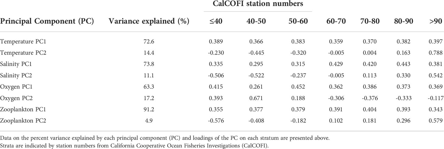
Table 1 Principal components analysis (PCA) performed on environmental variables binned by onshore-offshore strata.

Each oceanic variable’s principal component time series exhibited distinct temporal patterns (Figure 2). PC1 for temperature was primarily negative at the start of the time series, exhibited mainly positive values during the warm phase of the PDO between 1977-1998, displayed anomalies centered around zero during much of the 2000s and early 2010s, and rose sharply at the end of the time series in 2014-2015 coincident with MHW onset (Figure 2A; Di Lorenzo and Mantua, 2016). In contrast, PC1 of salinity was less closely correlated with the PDO, as has also been shown by Di Lorenzo et al. (2008). Instead, this PC exhibited greater variability at the interannual rather than decadal scale (Figure 2B). PC1 for DO was characterized by heightened variability at the start of the time series, with greater stability in more recent years (Figure 2C). Similar to the results for temperature, the PDO seemed to have a substantial influence on the zooplankton PC1 (Pearson correlation coefficient r=-0.49, p=0.0001, d.f. = 54). Zooplankton PC1 was characterized primarily by positive anomalies up until the mid-to-late 1970s and experienced a period dominated by negative anomalies after the PDO entered its warm phase (Figure 2D).

FIGURE 2

Figure 2 Time series of the first principal component of (A) temperature, (B) salinity, (C) dissolved oxygen (DO) concentration, and (D) mesozooplankton displacement volume from the southern California Current System. Note that there are some gaps in DO measurements during the early years of the CalCOFI time series. Horizontal, dashed lines indicate principal component scores of zero, while thick, vertical lines represent the timing of break points identified in time series. Gray bars show the posterior probability of a change point occurring each year in the time series of each oceanic variable. The winter Pacific Decadal Oscillation (PDO) is included as a blue line in (A) and its inverse is included as a turquoise line in (D) to illustrate correlations among principal components and this regional climate index.

The change point detection algorithm did not identify any regime shifts in the PC1 time series of temperatures, salinity, or DO. There was a 93.6% probability of zero change points detected in the temperature time series, 99.3% probability of zero salinity change points, and 63.7% probability of zero DO change points. In contrast, the posterior probability distribution indicated a 75.8% probability of two change points in the zooplankton PC1 time series, with 24.2% chance of one change point. The highest probabilities of change points were detected in 1968 and 1983. Prior to 1968, the PC1 time series for ZDV consistently exhibited positive anomalies (Figure 2D). During 1969-1983, ZDV was characterized by highly variable and declining abundance, while after 1983 this time series was fairly stable with anomalies close to zero.

3.1.2 SSB

With a posterior probability of 78.1%, one change point was detected in the time series of E. mordax SSB (Figure 3A). This change occurred in 1963, separating a period of low, but recovering SSB from a period when this species was fairly abundant. A decline in E. mordax biomass was observed at the end of this time, but there was only a 21.9% posterior probability that this decline was associated with a second change point.

FIGURE 3

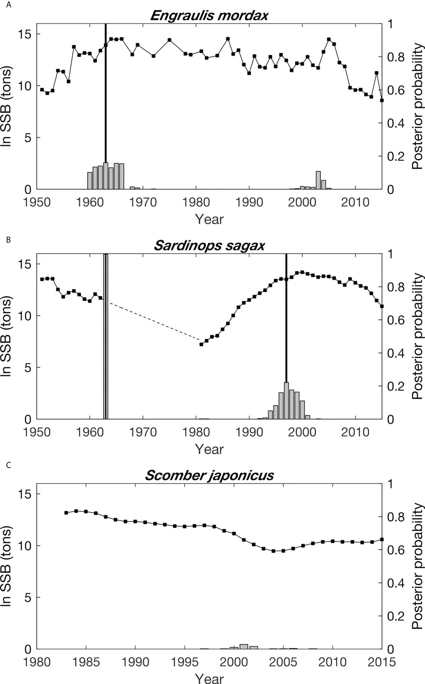
Figure 3 Time series of the natural log transformed spawning stock biomass (SSB) of (A) (E) mordax, (B) S. sagax, and (C) S. japonicus. No SSB data are available for T. symmetricus. Dashed line indicates the time period of low S. sagax biomass when no stock assessments were conducted to estimate this species’ SSB. Gray bars show the posterior probability of a change point in the SSB time series occurring each year. Black, vertical lines indicate the timing of break points identified in each time series.

For S. sagax, there was a 99.9% probability that its time series contained two change points, which were detected in 1963 and 1997 (Figure 3B). The 1963 change was associated with a decline in S. sagax biomass and its subsequent recovery. The precise date of this change is uncertain because of a discontinuity in the S. sagax time series due to a lack of stock assessments between 1964-1980. However, the fact that E. mordax also exhibited a change point during 1963 bolsters confidence in this result for S. sagax and suggests asynchronous dynamics between species. The second change point for S. sagax detected in 1997 was associated with stable, high fish biomass, with some declines near the time series end.

Log-transformed S. japonicus SSB was in decline throughout most of the period when biomass estimates were available (Figure 3C). With a posterior probability of 92.5%, no change points were detected for S. japonicus.

3.2 Non-stationarity detection using GAMs

Assessment of non-stationarity in models of all four species for each of the three types of regime shifts is described in the Supplementary Material 2.1-2.3 and Figures S3-11. Here we provide an in-depth, illustrative summary for one species as a case study and then compare general trends across all species and regime shift types.

3.2.1 Case study – changes points in S. sagax SSB

For each SSB regime, a single model was selected for S. sagax where the selected GAM had an Akaike weight >0.8 (Table S3). This indicated a >80% likelihood that the selected model was the most parsimonious choice of the candidate models.

Evidence of non-stationarity in how S. sagax relates to oceanic variables was found across all indicators. For the first indicator (inclusion of different variables in the selected GAM), non-stationarity was indicated by the fact that the model formulation changed across regimes. During the first two SSB regimes (1951-1963 and 1964-1997), temperature, salinity, and ZDV were included in the selected model, but DO was excluded (Table S2). In contrast, during the regime from 1998-2015, ZDV was excluded from the model.

The second indicator of non-stationarity was related to changes in whether fishes had linear or non-linear relationships with oceanic variables. In most models, the best-fit GAM included non-linear terms, with an edf of 3 (Table S2). Evidence of non-stationarity was observed since salinity initially had a linear relationship with larvae occurrence, which later became non-linear (Table S2; Figure 4).

FIGURE 4

Figure 4 Generalized additive model (GAM) response curves for S. sagax during three different spawning stock biomass (SSB) change points: 1951-1963 (A-D; blue), 1964-1997 (E-H; green), and 1998-2015 (I-K; red). Dashed lines indicate that 95% confidence intervals for each response curve. Missing subplots (log zooplankton during 1998-2015 and oxygen in 1951-1963 and 1964-1997) are indicative that a particular oceanic variable was not included in the most parsimonious GAM. Rug plots are displayed at the bottom of each subplot.

Non-stationarity changes in the ranked importance of oceanic variables were also observed. Ranking of salinity declined over time, while DO ranking increased (Figure 5J). Temperature and ZDV exhibited variability in their ranking, but without long-term trends.

FIGURE 5

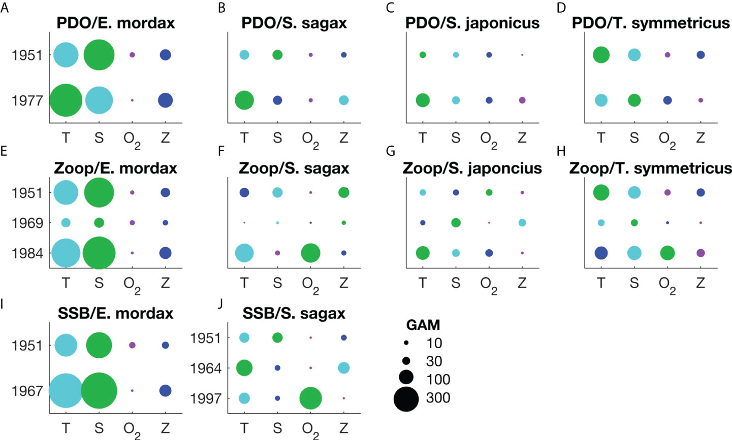
Figure 5 Rank order comparison between the influence of each oceanic variable on the presence/absence of larvae of E. mordax, S. sagax, S. japonicus, and T. symmetricus. Results are shown for change points designated based on changes in the sign of the Pacific Decadal Oscillation (PDO; A-D); break points in the mesozooplankton volume time series (E-H; the abbreviation “zoop” is used when labeling the title of these subplots), and; break points in the time series of E. mordax and S. sagax spawning stock biomass (SSB; I, J). Unless otherwise specified, time periods for each type of change point are the same across all species. Only the start year of a particular regime is listed here. Oceanic variables are abbreviated as follows: T – temperature, S – salinity, O₂ – dissolved oxygen concentration, Z – mesozooplankton volume. Comparisons between variables are based on the change in deviance (ΔD) when one variable is removed relative to the deviance of the full model. The scale for ΔD is shown in the lower, right corner of the figure. Note that ΔD is influenced by sample size so this metric is comparable across from a single regime, but not across multiple regime types due to variations in sample size. The rank order of different environmental variables for each period is shown based on circle size and color: green – 1^st rank, turquoise – 2^nd rank, blue – 3^rd rank, purple – 4^th rank.

Changes in response curve shape was the fourth indicator of non-stationarity. Temperature response curves had a negative, parabolic shape during the 1951-1963 and 1964-1997 regimes. During 1998-2015, the temperature response curve had a flatter shape, and a higher probability of encountering S. sagax larvae at low temperatures was observed (Figure 4). The flattened response curve shape during the third regime may indicate a reduced influence of temperature on sardine distribution, which is also consistent with changes in the relative ranking of temperature during this regime (Figure 5J). S. sagax were most frequently encountered at higher salinities throughout all periods, but the salinity response curve shape changed across periods. During 1951-1963, this species had a positive, linear relationship with salinity; during 1964-1997, this relationship had a negative, parabolic form; from 1998-2015, S. sagax distribution was less responsive to variations in salinity as indicated by a flattened response curve (Figure 4). Less change in response curve shape was observed for ZDV since it exhibited a negative, parabolic response curve during both periods when included in GAMs (Figure 4). Changes in curve shape could not be assessed for DO, since this variable was only included in the selected model during the third SSB regime.

Changes in the amplitude (or range) of the response curve was the fifth indicator of non-stationarity. A decrease in response curve amplitude is suggestive of a reduced influence of a variable on larval fishes. For temperature, response curve range was significantly larger during 1964-1997 than 1998-2015 (Figure 6I). The period when S. sagax was most sensitive to temperature based on this indicator coincided with low biomass of this species (Figure 3B). No significant changes were seen in response curve range for salinity and ZDV. Changes could not be assessed for DO since it was only included in the selected model during a single regime.

FIGURE 6

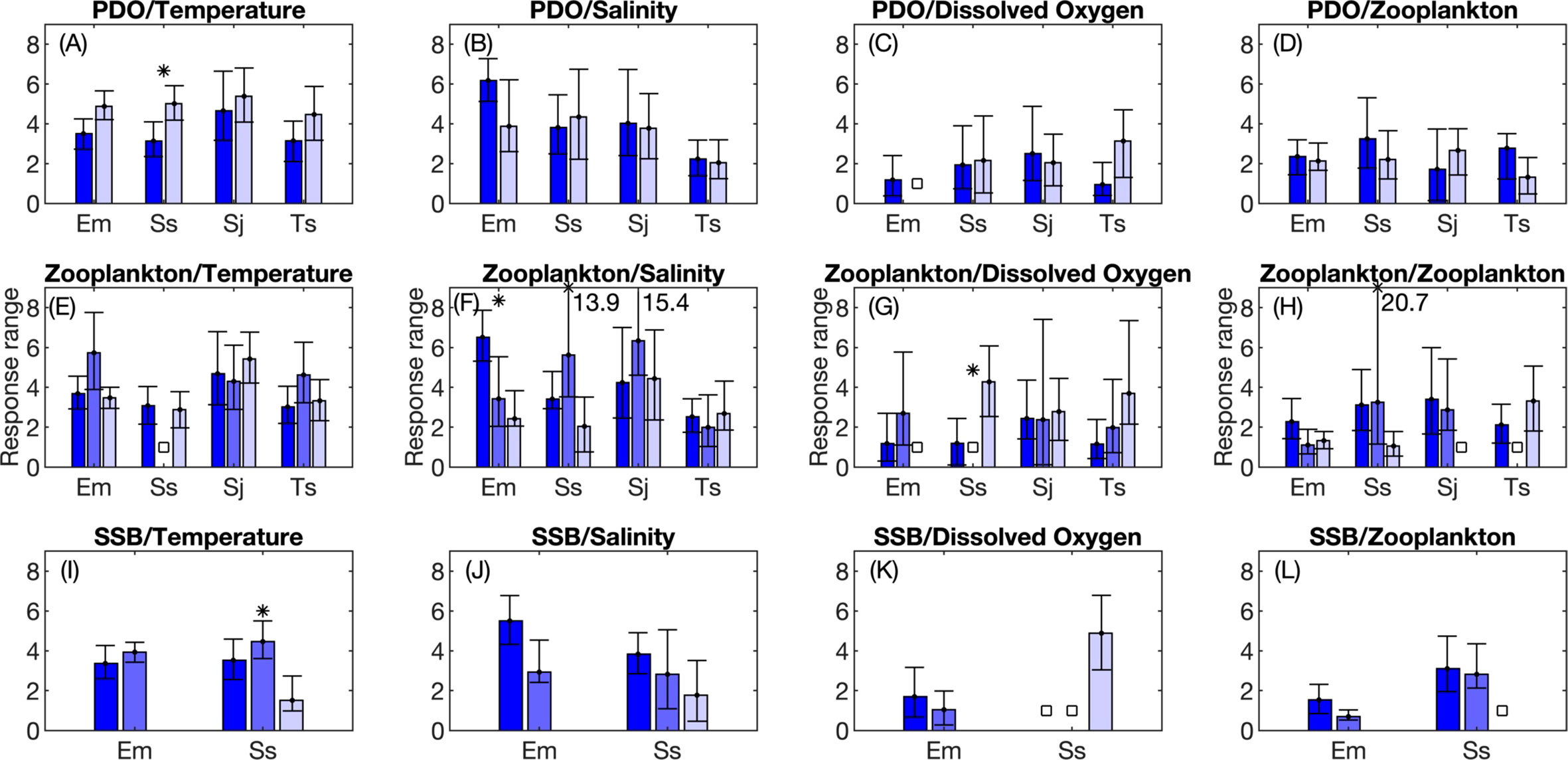
Figure 6 Changes between periods in the response curve range from generalized additive models (GAMs). Response curve range is defined as the difference between the maximum and minimum value in a GAM response curve and is indicative of how strongly an environmental variable influences larval fish occurrence. Median values and 95% confidence intervals from bootstrap analysis are shown. Results are shown for change points designated based on changes in the sign of the Pacific Decadal Oscillation (PDO; A-D); break points in the mesozooplankton volume time series (E-H), and; break points in the time series of E. mordax and S. sagax spawning stock biomass ( SSB; I-L). GAM results for different periods are displayed in groups, with the first period represented by the left most bar in a group (dark blue color) and the last period displayed to the right (light lavendar color). Intermediate periods are displayed in the middle of each group. Stars (*) indicate that periods are significantly different from each other for a given species and environmental variable based on non-overlapping 95% confidence intervals. White squares indicate that a particular variable was not included in the best fit GAM model(s). Numbers shown in some subplots indicate the maximum response curve range in a few cases where the maximum value exceeds the y-axis limit of a graph. Species names are abbreviated based on the first letter of the genus and the first letters of the species name: Em, Engraulis mordax; Ss, Sardinops sagax; Sj, Scomber japonicus; Ts, Trachurus symmetricus.

Significant changes in the sixth indicator of non-stationarity (shifts in the peak of the response curve) were observed for several oceanic variables. For temperature, S. sagax was most commonly found in areas with significantly cooler temperatures during 1998-2015 compared to prior periods (Figure 7I). The maximum likelihood of detecting larvae occurred at significantly lower salinities in 1964-1997 than 1951-1963 (Figure 7J). Sardine larvae were found in areas with significantly less zooplankton during 1964-1997 than 1951-1963 (Figure 7L). Since the former period was characterized by reduced ZDV (Figure S1), this might reflect a change in the availability of zooplankton rather than an active shift in habitat selection.

FIGURE 7

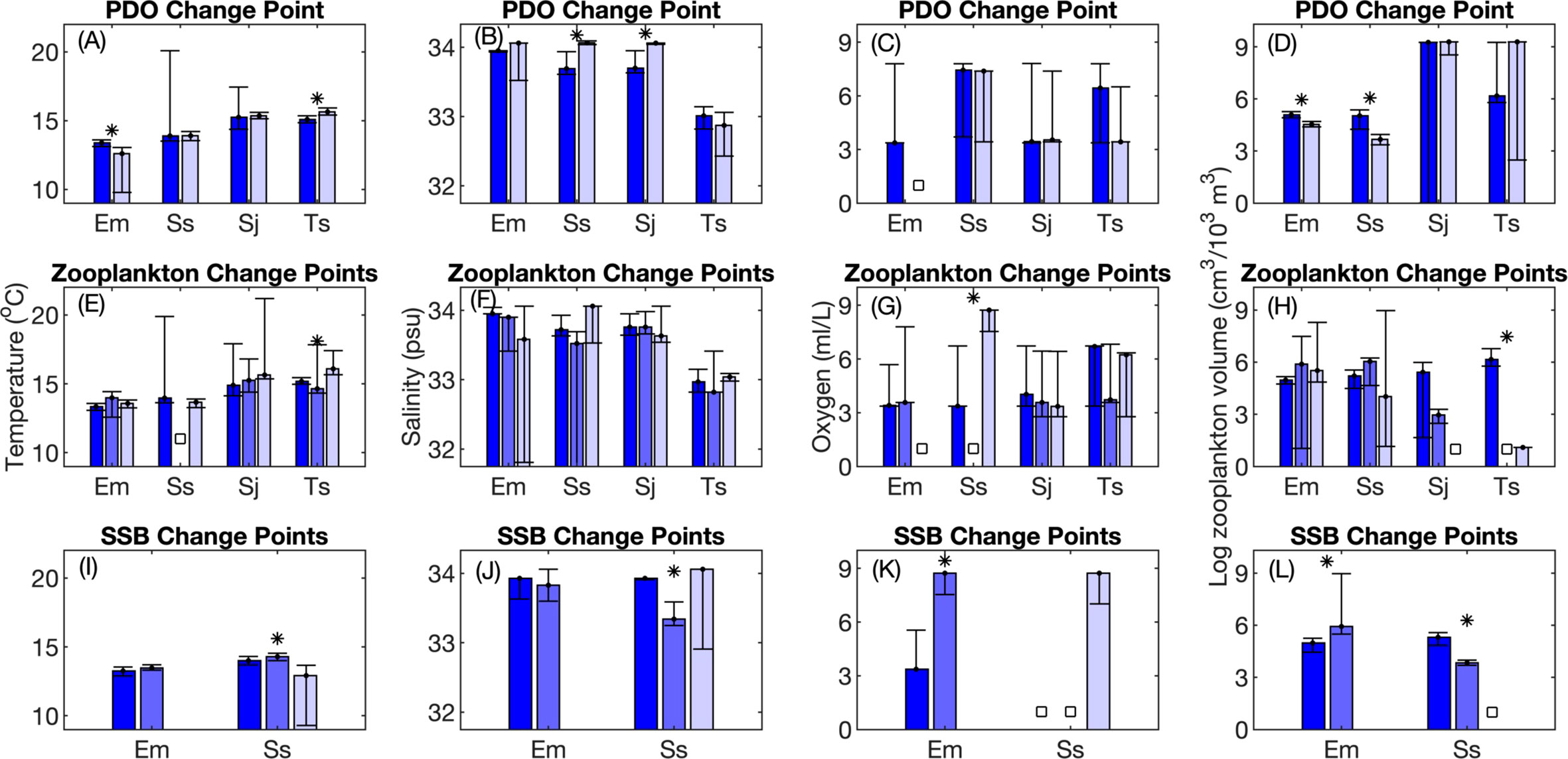
Figure 7 Changes between periods in the peak value of generalized additive model (GAM) response curves. The peak in response curves is indicative of the environmental conditions that maximize the likelihood of occurrence of E. mordax, S. sagax, S. japonicus, and T. symmetricus. Median values and 95% confidence intervals from bootstrap analysis are shown. Results are shown for change points designated based on changes in the sign of the Pacific Decadal Oscillation (PDO; A-D); break points in the mesozooplankton volume time series (E-H), and; break points in the time series of E. mordax and S. sagax spawning stock biomass (SSB; I-L). Bar colors, symbols, and species name abbreviations are the same as in Figure 6.

3.2.2 Comparisons across species and regime shift types

Every combination of species and regime type exhibited at least one indication of non-stationarity, implying that non-stationarity is ubiquitous across SPF in the CCS. A summary of patterns observed across non-stationarity indicators, oceanic variables, species, and regime types is included below.

A change in oceanic variables included in GAMs was observed across 60% of the combinations of species and regime shifts (Table 2). Nearly half of the selected of the selected models contained all four environmental variables, but in several cases the most parsimonious model(s) excluded DO or ZDV (Table S2). In a smaller number of cases, a simplified model containing 1-2 environmental variables was selected.

TABLE 2

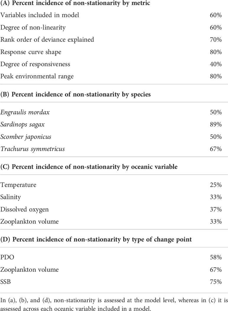
Table 2 Percent incidence of non-stationarity by indicator metric, species, oceanic variable, and change point type for generalized additive models (GAMs).

Changes in the linearity of the relationship between fishes and environmental variables also occurred across 60% of the combinations of species and regime shifts (Tables 2, S2). Salinity and DO were the most common variables to exhibit changes in linearity.

Changes in the ranked importance of oceanic variables were very common, with evidence of non-stationarity occurring across all species (Figure 5). Temperature and salinity were frequently ranked as having the greatest or second greatest influence on fish larvae, with lower rankings more common among DO and ZDV. Among S. sagax and T. symmetricus, the relative ranking of DO increased during recent periods.

Changes in response curve shape were observed across 80% of species and regime combinations (Table 2). The only cases where pronounced changes in response curve shape were not detected was among shifts between PDO phases for E. mordax and S. japonicus (Figures S3, S5). Of the four oceanic variables, temperature was the least likely to have a change in response curve shape, usually displaying a negative, parabolic shape (Figures 4, S3-S11). Like temperature, ZDV often exhibited a negative, parabolic response curve shape, especially at the start or mid-point of time series. In many cases (e.g., Figures S6-S8, S11), ZDV response curves displayed a flatter shape during later periods, indicating a reduced influence of this variable. The response curves for salinity and DO usually displayed wide confidence intervals at extrema, indicating reduced certainty in how fishes respond to these variables under conditions deviating from the mean. Lastly, compared to other species, S. sagax displayed a greater propensity for changes in response curve shape (Figures 4, S4, S8).

The amplitude of response curves, which is an indicator of sensitivity to oceanic variables, displayed non-stationarity across four of the ten combinations of species and regime shifts (Table 2). Only one significant change in this indicator was observed across PDO and SSB regimes, whereas deviations from stationarity were more common among zooplankton regimes (Figure 6). Deviations from stationarity for this indicator were most common among S. sagax.

Shifts in peak habitat use tied other indicators for the second most incidences of non-stationarity. This indicator refers to changes in the range of environmental variables associated with maximum larval occurrence. For 80% of species and regime shift combinations, at least one oceanic variable exhibited non-stationarity for this indicator (Table 2). Multiple species exhibited changes in the temperature and salinity at which their response curve peaked (Figure 7), but no overarching pattern of change between periods was identified amongst these variables. In contrast, whenever there was a significant change in peak DO use, fishes tended to occur in areas with higher DO in more recent years (Figures 7G, K). In four out of five cases where there was a significant change in peak use of ZDV, fishes occurred in areas with less ZDV during more recent years (Figures 7D, H, L). This may be related to long-term declines in ZDV in this ecosystem (Roemmich and McGowan, 1995; Lavaniegos and Ohman, 2007). Compared to other species, S. sagax was most likely to display significant changes in this indicator.

When integrating across all indicators, S. sagax was the species whose relationship with oceanic variables displayed the most signs of non-stationarity (Table 2). S. japonicus and E. mordax displayed the fewest indications of non-stationarity, even though some non-stationarity was detected for them across >50% of the indicators and regime shift types. Non-stationarity was most common among salinity and DO, whereas the relationship between fish presence/absence, temperature, and ZDV exhibited slightly more stability. Among different regimes, non-stationarity was observed most frequently for SSB regimes when integrated across indicators (Table 2).

3.3 Future projections

CNRM-ESM2 was used to produce end of the 21^st century projections of suitable habitat for larval fishes and assess whether these projections differed significantly depending on which ecological or climatic regime was used to parameterize projection models. For E. mordax, S. sagax, and S. japonicus, habitat suitability declined during future projections, with a steeper loss in suitable habitat under SSP5-8.5 (Figure 8). For this scenario, decreases in mean IHS varied between 40.5-90.8% relative to the historical baseline. Under SSP1-2.6, declines in suitable habitat never exceeded 53.1% for any species or regime. In contrast to other species, T. symmetricus habitat suitability was projected to increase under SSP1-2.6 and SSP5-8.5 during spring (Figures 8D, H).

FIGURE 8

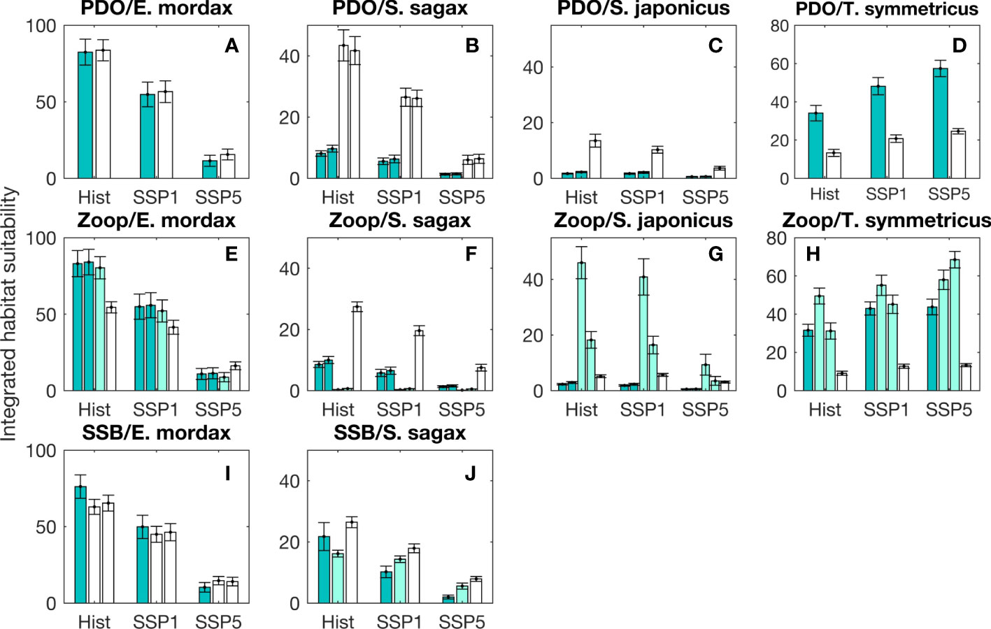
Figure 8 Integrated habitat suitability (IHS) for larval fishes during spring months based on projections from the CNRM Earth System Model (CNRM-ESM-2-1). Annual mean IHS scores (± 95% confidence intervals) are shown for a historical simulation for the years 1980-1999 (abbreviated as Hist) and two future simulations (SSP1-2.6 and SSP5-8.5) for the years 2080-2099. Using the climate forcing from each CNRM-ESM-2-1 simulation, habitat suitability was projected based on generalized additive models (GAMs) parameterized with data from different regimes and species. Results are shown for change points designated based on changes in the sign of the Pacific Decadal Oscillation (PDO; A-D); break points in the mesozooplankton volume time series (E-H; abbreviated as Zoop), and; break points in the time series of E. mordax and S. sagax spawning stock biomass (SSB; I, J). GAM results for different periods are displayed in groups, with the first period represented by the left most bar in a group (green color) and the last period displayed to the right (white color). Intermediate periods are displayed in the middle of each group (pale green color). In cases where multiple models were selected for a particular regime, separate bars are shown for each model using the color coding described above.

Two-way ANOVAs indicated that GAM model choice had a significant effect on habitat suitability in most cases (Table 3). The two exceptions to this occurred among E. mordax during regimes defined by PDO and SSB changes. For most species and regime shift types, F statistics from ANOVAs were larger for the GAM effect than the SSP effect, implying that the period used to parameterize the GAM had a larger impact on habitat suitability than SSP scenario. Furthermore, most species exhibited significant interactions between SSPs and GAMs from different regimes. One common pattern among interaction terms was that GAMs parameterized during periods with greater habitat suitability tended to undergo larger changes under future climate scenarios.

TABLE 3

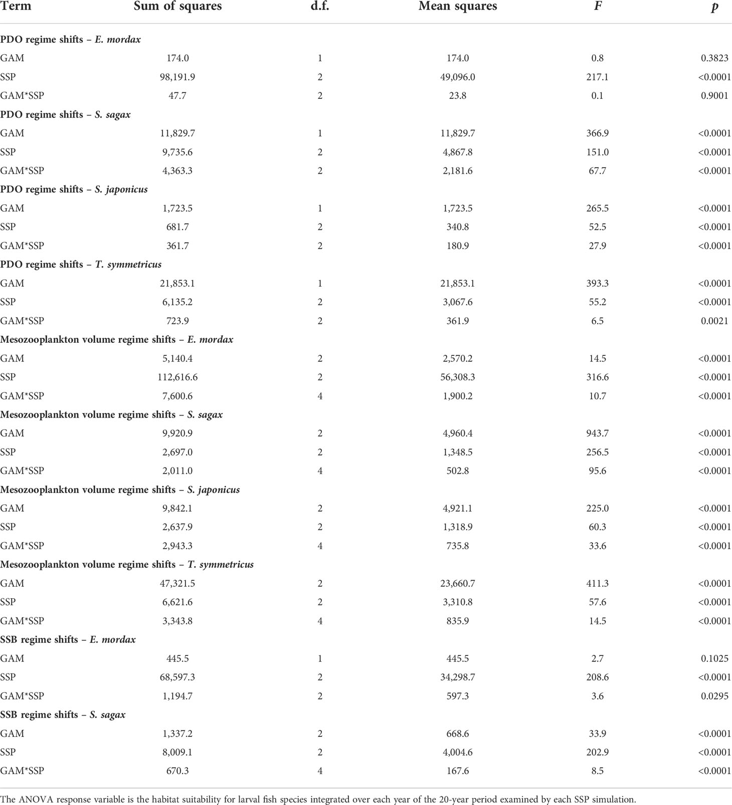
Table 3 Two-way crossed analysis of variance (ANOVA) examining interactions between shared socioeconomic pathway (SSP) simulations and projections from generalized additive models (GAMs) trained during different ecological and climatic regimes.

Changes in the mean CV between the historical and SSP5-8.5 scenarios were assessed to determine if variability in suitable habitat may increase under climate change. Increased variability was observed for all species, except T. symmetricus, under SSP5-8.5 (Table 4A). Variance in IHS was greater under regimes defined by changes in ZDV than other types of regimes (Table 4B). Regimes characterized by non-stationarity in salinity and ZDV exhibited greater variability than regimes with non-stationarity in temperature and DO (Table 4C). However, many regimes exhibited concurrent non-stationarity across multiple environmental variables, making it challenging to partition these effects among variables. The largest increases in variability under climate change were observed when there was non-stationarity associated with shifts in which variables were included in GAMs and changes in response curve amplitude (Table 4D).

TABLE 4

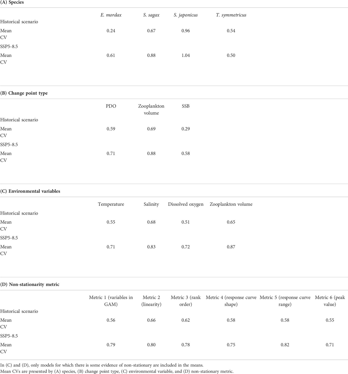
Table 4 Mean coefficient of variation (CV) for GAM model projections of annual integrated habitat suitability (IHS) under the historical and SSP5-8.5 climate scenarios.

4 Discussion

Non-stationary relationships between organismal distribution and climate can result in inaccurate projections of how species respond to climate change, but this subject has not been widely investigated across ecosystems (Litzow et al., 2019). We found that indications of non-stationarity were nearly ubiquitous among SPF species when models were constructed for three types of regime shifts. Non-stationarity most frequently resulted in changes in response curve shape, shifts in the peak range of conditions where larvae occurred, and changes in the relative importance of oceanic variables. Non-stationarity was most frequently associated with changes in ecological conditions, such as shifts in fish SSB or ZDV, rather than changes in the PDO. Relationships between fishes and temperature were more stable than other environmental variables. This might partially reflect greater uncertainty in relationships between fish distribution, salinity, and DO, which is indicated by the large confidence intervals associated with these variables’ response curves. For several combinations of regimes and species, DO had a greater influence on distribution in recent years (Figures 5, 7). Often the effects of non-stationarity on larval habitat suitability were larger than changes projected under high and low greenhouse gas emissions.

4.1 Non-stationary fish-environment relationships

Among fishes, non-stationarity can affect how environmental factors influence species distribution, recruitment, and fisheries productivity. Here we integrate our discussion across these types of non-stationarity. While non-stationarity has not been frequently considered in the scientific literature, when it has been investigated, results are similar to ours in that changes in organismal-environmental relationships are widespread. In studies comparing whether fish and invertebrate density, biomass, recruitment, and catch can be best modeled with stationary or non-stationary models, there is a pattern where the best fit model is usually non-stationary (Ciannelli et al., 2007; Lindegren and Eero, 2013; Beggs et al., 2014; Litzow et al., 2018; van der Sleen et al., 2018; Puerta et al., 2019). Similar results have been seen among non-marine taxa. For example, among British butterflies, changes in distribution in response to warming were not consistent across periods (Mair et al., 2012).

Among SPF, non-stationarity has been observed in multiple ecosystems and may be related to the boom-bust cycles of abundance common to this functional group. In the Northwest Atlantic, Atlantic menhaden (Brevoortia tyrannus) occurrence has a non-stationary relationship with temperature modulated by the North Atlantic Oscillation (Roberts et al., 2019). Changes in sardine (S. sagax) and anchovy (E. encrasicolus) spawning habitat preferences in the southern Benguela could be partially, but not fully, explained by warming, suggesting non-stationarity relationships occur among these stocks (Mhlongo et al., 2015). Among Japanese anchovy (E. japonicus), temperature where fish occurred as eggs and larvae differed between 1978-1991 and 1992-2004, which is suggestive of non-stationarity (Takasuka et al., 2008).

It is unclear whether SPF are more likely to exhibit non-stationary dynamics than other fishes. SPF are adapted to environments with a high degree of climate variability (Checkley et al., 2017), which could be indicative of resilience to fluctuating conditions. Conversely, SPF are more subject to population collapse than other fishes (Pinsky and Byler, 2015), suggesting highly non-linear and unstable dynamics. Fernandes et al. (2020) showed that SDMs have a reduced capacity to predict the normalized biomass of pelagic species compared to benthic species. However, the mechanism behind this observation is unclear and could be due to either greater non-stationarity among pelagic fishes or differences in sampling efficacy.

4.1.1 Non-stationarity in the California Current System

Within the CCS, evidence has previously suggested that non-stationarity may be common among S. sagax, but much less research has investigated dynamics of other SPF. One early publication indicating that S. sagax has a variable relationship with environmental conditions is Lynn (2003) who found that SST delimits the northern extent of S. sagax spawning habitat, but that the specific limit differs between years. Several studies have documented that the relationship between temperature and S. sagax recruits per spawner is sensitive to time period and source of temperature data (Jacobson and MacCall, 1995; McClatchie et al., 2010; Lindegren and Checkley, 2012; Zwolinski and Demer, 2019). Muhling et al. (2020) found indications of non-stationarity for S. sagax during the 2014-2017 MHW when fish occurred at temperatures warmer than projected by SDMs. Our results expand upon Muhling et al. (2020) by identifying changes in the sensitivity of S. sagax to environmental variables during earlier periods, indicating that non-stationarity during the MHW was not solely due to the inability of S. sagax to avoid unfavorable habitats during rapid change. Our results also confirm that non-stationarity among S. sagax can occur in absence of novel environmental conditions, such as those associated with an MHW. Instead, non-stationarity likely emerges due to interplay between multiple factors (e.g., variations in population size, prey availability, interactions between oceanic conditions, shifts in where and when fish spawn).

Our results help explain some contradictions between earlier publications on SPF spawning habitat. There is generally a consensus that the northern stock of S. sagax spawns at 12-16° C, with several publications indicating peak spawning at temperatures around 13-14° C (Checkley Jr et al., 2000; Lynn, 2003; Reiss et al., 2008; Zwolinski et al., 2011; Asch and Checkley Jr, 2013). Our results are consistent with this consensus, although there are variations between periods in how quickly optimal spawning habitat declines at temperatures moving away from this peak. E. mordax generally spawn at 12-18° C, but the exact range of temperatures occupied by this species varies between studies, which may reflect variations in the rate at which response curves decline moving away from peak temperatures (Fiedler, 1983; Lluch-Belda et al., 1991; Checkley Jr et al, 2000; Reiss et al., 2008; Weber and McClatchie, 2010; Asch and Checkley Jr, 2013). Checkley Jr et al. (2000) and Asch and Checkley Jr (2013) found that S. sagax eggs were most frequently observed at intermediate salinities of 33.0-33.4 psu, whereas Weber and McClatchie (2010) identified a monotonically decreasing relationship between S. sagax larvae and salinity. This contradiction likely reflects the fact that each study considered a different period since the shape of salinity response curves is sensitive to the years used to parameterize SDMs. In contrast, all previous research including ours indicate that E. mordax spawn at higher salinities in the southern CCS (Checkley Jr et al., 2000; Weber and McClatchie, 2010; Asch and Checkley Jr, 2013). However, given that this species resides in the Columbia River freshwater plume in the northern CCS (Kaltenberg et al., 2010), phenotypic plasticity or local adaptation might influence E. mordax larval occurrence with regard to salinity. Different studies have identified positive and negative relationships between S. sagax and zooplankton concentration (Checkley Jr et al., 2000; Lynn, 2003; Agostini et al., 2007). While this might reflect differences in the life stage of S. sagax studied, variations in zooplankton species composition, or spurious correlations, non-stationary relationships provide an alternative explanation.

Less research has been conducted on the relationship between SPF and DO in the southern CCS. Koslow et al. (2013) suggested that there was a positive relationship between DO and S. sagax larvae, which is consistent with our results across the majority, but not all, regimes. Howard et al. (2020) indicated that the distribution of E. mordax is sensitive to DO, especially at high temperatures, which is comparable to our results from recent years, although other patterns are seen early in the CalCOFI time series. These two papers mainly focused mid-water column depths because projected declines in DO concentration under climate change are maximized across this range (Dussin et al., 2019). Our research focused on environmental conditions in the upper 50 m of the water column coincident with the peak vertical distribution of SPF eggs and larvae. Since hypoxic conditions at these depths only occur during extreme upwelling, the reaction of SPF larvae to DO in our study is more representative of the influence of DO as an indicator of water mass characteristics rather than as a physiological stressor.

Less research has been conducted on environmental influences on the species distribution of S. japonicus and T. symmetricus in the southern CCS. Our results are consistent with prior studies of the influence of temperature and salinity on their spawning distribution (Weber and McClatchie, 2012; Asch and Checkley Jr, 2013). However, this is less so for ZDV. For S. japonicus, Weber and McClatchie (2012) found that larvae were most likely to be present at intermediate ZDVs of ~5-7 log cm³ 1,000 m^-3. While we observed a similar relationship between ZDV and S. japonicus larvae during 1951-1968 (Figure S9), this pattern was not apparent in other periods. Asch and Checkley Jr (2013) identified the highest probability of T. symmetricus eggs at low ZDV. The current study identified a similar pattern during 1984-2015, which coincides with years examined by Asch and Checkley Jr (2013). However, differing relationships between T. symmetricus distribution and ZDV were observed during earlier periods.

T. symmetricus was the only species to experience a projected increase in IHS under SSP1-2.6 and SSP5-8.5. We hypothesize that this increase in suitable habitat is related to a shift in spawning phenology of T. symmetricus under climate change. Future projections were made for March-May since an empirical formula for converting between mesozooplankton carbon biomass from CNRM-ESM2 to ZDV was only available for this season (Supplementary Material 1.2). While these months coincided with the seasonal peak in larval concentration for E. mordax, S. sagax, and S. japonicus, maximum concentrations of T. symmetricus are observed in June (Moser et al., 2001). Asch (2015) identified T. symmetricus as belonging to a group of fishes whose phenology has become earlier in recent decades in response to warming. The projected future increase in habitat suitability for T. symmetricus during March-May likely represents a continuation of this shift towards earlier spawning phenology.

Since fish-environmental relationships change over time, this emphasizes the importance of accurately detecting timing of regime shifts. Our study analyzed change points associated with the 1976/1977 PDO phase change, 1968/1969 and 1983/1984 shifts in ZDV, changes in S. sagax and E. mordax SSB in 1963/1964, and a second shift in S. sagax SSB in 1997/1998. No change points were detected in time series of temperature, salinity, and DO, which may reflect that biological time series often have more non-linear dynamics than physicochemical variables (Hsieh et al., 2005). The change points detected were well supported by other studies of the southern CCS. The 1976/1977 PDO transition was associated with reduced survival young-of-year E. mordax (Nishikawa et al., 2019). The presence of a mid-1960s regime shift was consistent with an analysis of 35 species of CCS ichthyoplankton (Peabody et al., 2018). Other ichthyoplankton studies have identified faunal shifts during 1983/1984 and the late 1990s (Miller and McGowan, 2013; Peabody et al., 2018; Thompson et al., 2019a), which approximately coincide with our change points in ZDV and S. sagax SSB, respectively. Unlike previous studies, we did not detect a 1989/1990 regime shift (Miller and McGowan, 2013; Koslow et al., 2015; Peabody et al., 2018). This might reflect that this change point seems to be principally associated with shifts among a few highly abundant taxa in the southern CCS (Peabody et al., 2018). Our Bayesian change point algorithm indicated that there was some uncertainty in the exact year of transitions (Figures 2, 3). This uncertainty may reflect gaps in CalCOFI time series coverage, discontinuities in stock assessments, the decision to log-transform SSB prior to change point detection, and uncertainty related to parameter choice during change point detection (Overland et al., 2008; Peabody et al., 2018). For instance, the choice of minimum regime length affects detection of recent ecological shifts, such as the crash and subsequent recovery of E. mordax (Thayer et al., 2017; Thompson et al., 2019b).

4.2 Mechanisms responsible for non-stationary dynamics

Currently there is limited capacity for predicting the occurrence of non-linear ecosystem regime shifts. A meta-analysis of 4,600 global change impacts concluded that such shifts were rarely detectable in advance (Hildebrand et al., 2020). While many regime shifts are characterized by increased time series variance (Lenton, 2011), this signal can be obscured by small variations in organismal responses (Hildebrand et al., 2020). Similarly, Field et al. (2009) concluded that fluctuations in SPF abundance in paleo-ecological time series were characterized by red noise that was not predictable. When combined with novel environmental conditions and changes in how fish react to oceanic variables across regimes, these factors challenge the ability of empirically derived models to make accurate future projections needed for management. However, models that incorporate physiological principles and mechanistic ecological understanding may fare better.

While our study did not directly investigate mechanisms responsibility for non-stationarity, some insights can be attained and may help generate hypotheses for future research. Given the greater amount of literature on S. sagax and E. mordax, more hypotheses exist to explain non-stationary dynamics among these species. Previous studies suggested that the relationships between these fishes and SST may be a proxy for other environmental factors (e.g., prey availability) that more directly influence population dynamics (Fiedler, 1983; Jacobson and MacCall, 1995). This could lead to non-stationarity if relationships between SST and the direct influences on a species become decoupled. However, this seems unlikely to explain the non-stationarity observed here because the relationship between temperature and larval habitat exhibited greater stationarity than other variables. Previous studies have indicated that DO in the CCS is correlated with variations in nutrient and chlorophyll concentration, water mass characteristics, and geostrophic flow (Weber and McClatchie, 2010; Koslow et al., 2013). Since the relationship between DO and larval presence/absence was subject to greater non-stationarity, changes in the strength of these correlations could be possibly responsible for this non-stationarity.

Changes in modes of climate variability and trophodynamic relationships have also been hypothesized to be mechanisms responsible for non-stationarity in SDMs (Litzow et al., 2019). We observed slightly more non-stationarity across zooplankton regime changes than PDO shifts, suggesting support for trophodynamic changes as an underlying cause of non-stationarity. Related to this point, it must be noted that an environmental variable needs to exceed an organism’s tolerance range to affect its distribution. Under modes of climate variability that are favorable to an organism, this tolerance range might not be exceeded. However, values outside of their tolerance may be experienced by fishes during the opposite phase of climate variability or as the climate continues to change. This mechanism could lead to the appearance of non-stationarity when using SDMs parameterized with data from different periods.

Additional mechanisms for explaining non-stationarity are related to migration and dispersal. Since larvae are subject to advection, they do not have complete control over habitats occupied, which could increase the likelihood of non-stationarity (Brun et al., 2016). Conversely, movement by adults can help fishes track favored environmental conditions whereas less migratory species may be unable to follow such conditions (Reglero et al., 2012). This would imply that less migratory species may be subject to greater non-stationarity. However, migratory species may be equipped to face a greater variety of conditions encountered along migration pathways, implying that their distribution may be less tightly coupled with oceanic conditions. S. sagax displays greater seasonal migratory behavior than E. mordax (Zwolinski et al., 2011) and exhibited a greater incidence of non-stationarity. This suggests the latter idea (i.e., migratory behavior is associated with fewer environmental distribution constraints) has more support based on our data. Our results are also consistent with Planque et al. (2007); Weber and McClatchie (2010), and Muhling et al. (2020) who found that E. mordax distribution could be better fit by SDMs than S. sagax. S. sagax tends to exhibit greater variability in distribution than E. mordax at interannual-to-decadal scales, expanding its distribution offshore and northward when abundant (MacCall, 1990). This expansion, hypothesized to be driven by density-dependent habitat use, may be responsible for greater non-stationarity among S. sagax.

Beyond migratory behavior, there are at least two other hypotheses that could explain the high degree of non-stationarity among S. sagax. This species is known to undergo demographic changes as its abundance fluctuates. S. sagax reaches maturity at age 1 under low biomass and matures at age 2 at high biomass (Hill et al., 2008). Such demographic changes can increase the sensitivity of species to environmental variability (Anderson et al., 2008), which could generate non-stationarity. Another potential explanation could be related to intermixing between the U.S. and southern Baja California stocks of S. sagax, which use distinct thermal habitats (Lynn, 2003; Dorval et al., 2011). Nonetheless, the thermal history of habitat occupancy recorded in S. sagax otoliths from the southern CCS suggests intermixing of stocks is somewhat rare (Dorval et al., 2011).

4.3 Non-stationarity among oceanic variables

Climate change projections for marine organisms may be improved by focusing on oceanic variables less likely to exhibit non-stationarity. Of the variables considered, temperature most frequently exhibited stable relationships with larvae distribution (Table 2). This reflects that temperature has a direct influence on biological processes as diverse as gene expression, enzyme kinetics, metabolism, consumption, and growth in poikilotherms (Hare et al., 2012). Most marine fishes do not change their mean temperature of occurrence over time (Nye et al., 2009) and track climate velocity by shifting their distribution and depth to reflect changing temperatures (Pinsky et al., 2013). Rates of evolution of thermal niches are projected to be much slower than rates of future environmental change, leading to niche conservatism (Jezkova and Wiens, 2016). Consequently, SDMs driven by thermal preferences may be more reliable for making future projections than those with substantial influences from other variables. Nonetheless, multivariate SDMs generally are better at predicting historical distribution than univariate models (McHenry et al., 2019).

Salinity and ZDV exhibited an intermediate-to-high amount of non-stationarity. Species were often less responsive to these variables during recent regimes as indicated by exclusion of these variables from models, flattened response curves, or decreases in their ranking (e.g., Figures 4, 5). For ZDV, in some cases, fishes were less likely to display a unimodal response curve in recent years. Some non-stationarity observed among these variables may be related to the fact that their response curves had wider confident intervals near the minima and maxima of observed conditions. Due to wide confidence intervals, it was not always possible to determine whether changes in response curves between regimes represented changes in larval occurrence or solely a lack of capacity to precisely quantify responses to infrequently observed states. Brun et al. (2016) obtained similar results where SDMs displayed decreased skill near the edges of a species range where conditions were more extreme. It is important to understand how species react to such extremes since they are projected to occur more frequent under climate change (Frölicher et al., 2018). Laboratory experiments may be useful since they allow for replication of extremes observed infrequently in nature.

DO often exhibited a greater influence on SPF during recent regimes (Figures 5, 6, S2). Under climate change, DO in the CCS is projected to decline due to reduced solubility of oxygen in warmer water, increased stratification, changes in deep-water circulation causing reduced ventilation, and changes in upwelling strength (Rykaczewski and Dunne, 2010; Dussin et al., 2019). These changes have been documented to influence the historical abundance of mesopelagic fishes in the southern CCS (Koslow et al., 2011) and are projected to affect the future persistence of E. mordax in the region (Howard et al., 2020). Our findings are consistent with these patterns.

4.4 Projection uncertainty

For climate change impacts to be considered in fisheries management, uncertainty in future projections must be quantified. This is because managers will need to contemplate both best- and worst-case scenarios in the planning process (Cheung et al., 2016a). In ecological models, uncertainty can result from incomplete observational records, different approaches to conceptual and numerical model formulation, parameter estimation, model selection, choice of spatiotemporal scale, and adaptability of living systems (Planque et al., 2011). Future research should consider non-stationarity in fish-environmental relationships as another source of model uncertainty. Here we showed that the period used to parameterize SDMs can have a substantial impact on future projections due to non-stationarity, with the magnitude of this effect sometimes exceeding the effect of different climate scenarios. One understudied area with respect to climate change uncertainty is whether there might be interactions between different sources of uncertainty. We found that an interaction exists between uncertainty due to non-stationarity and SSP scenario, with an increasing effect of non-stationarity at higher emissions.

As with most SDMs, there are a number of qualifications that may affect our results. To take advantage of the multi-decadal CalCOFI time series, our analysis focused on the southern CCS, which does not encompass the full range of target species. Nonetheless, given the pronounced onshore-offshore gradients sampled by CalCOFI, this dataset covers several oceanic water masses exhibiting different conditions (McClatchie, 2013). Also, previous research has used CalCOFI to understand how environmental change affects fish distribution despite the dataset’s limited spatial extent (Hsieh et al., 2008; Hsieh et al., 2009; Howard et al., 2020; Muhling et al., 2020). A second qualification is that some of the changes in how fishes respond to the environment could be related to interactions between multiple variables influencing fish distribution. Changes in response curve shape may reflect the fact that partial responses from GAMs depend on the partial response of a species to other variables. For example, the extent to which DO is a stressor depends on temperature (Howard et al., 2020). GAMs often do not account for such interactions, but other SDMs do. We evaluated non-stationarity across periods with change points in S. sagax SSB using a second model that accounts for such interactions (the non-parametric probabilistic ecological niche model; Beaugrand et al., 2011; R.G. Asch unpublished data). Since non-stationarity was also common when using this alternative SDM, the high incidence of non-stationarity in the GAMs cannot be explained solely by multivariate interactions. Our models purposely did not include SSB as an independent variable because it is unlikely that future SSB would be precisely known when projecting climate change impacts. However, SSB can influence S. sagax and S. japonicus larval distribution (Weber and McClatchie, 2010; Weber and McClatchie, 2012). Models may display fewer incidences of non-stationarity due to density dependence if different SSB scenarios are included in long-range projections. Another critique of SDMs is that they do not typically allow for acclimation or adaptation to changing conditions. However, it is also unclear how important these processes are for fishes since thermal niches evolve slowly (Jezkova and Wiens, 2016). Also, fishes may migrate towards preferred conditions prior to acclimation (Habary et al., 2016).

4.5 Recommendations for improving SDM projections for marine fishes

Moving forward, it is important to determine if the high incidence of non-stationarity detected here is widespread or mainly a characteristic among SPF larvae in upwelling systems. For populations likely subject to non-stationary environmental relationships, we recommend validating SDMs with independent datasets whenever possible. Cross-validation with a subset of the original dataset can result in potential overestimation of model skill due to temporal and spatial autocorrelation or overfitting (Araújo et al., 2005; Planque et al., 2011). Some measures of model skill, such as the true skill statistic, perform similarly regardless of the time lag between datasets used for model development and testing (Brun et al., 2016). Wider use of the true skill statistic could help realistically assess model skill when an independent dataset is unavailable for validation. Since variables exhibiting indications of non-stationarity were more likely to have SDM response curves with wide confidence intervals, we recommend that response curve confidence intervals be more frequently reported. Nonetheless, some climate-envelope models may underestimate confidence intervals associated with the centroid of species distribution (Thorson, 2018).

Another suggestion for guarding against non-stationarity and improving confidence in SDM projections is to compare model-derived environmental niches against those from physiological experiments (Asch and Erisman, 2018; Muhling et al., 2020). Alternatively, physiologically based thermal tolerances can be used to parameterize SDMs (Hare et al., 2012). However, it is not unusual to see discrepancies between laboratory-derived and field-based estimates of thermal niche due to differences between fundamental and realized niches (Henderson, 2019). Related to this, fishes may not fully occupy suitable habitat within their realized niche during low abundance (Planque et al., 2007), which can lead to non-stationary relationships. Using thresholds GAMs where a threshold is prescribed based on fish biomass is a common way to mitigate against such dynamics (Lindegren and Eero, 2013; Beggs et al., 2014; van der Sleen et al., 2018).

Obtaining reliable projections of fish species distribution, phenology, and population dynamics is important, because it allows fisheries managers to better engage in adaptive management. Networks of marine protected areas and the timing of seasonal fishing closures may need adjustment as fishes undergo range shifts or phenological changes (McLeod et al., 2009; Peer and Miller, 2014). Fisheries independent surveys can be made more efficient when relationships between fish distribution and the environment are used to adaptively adjust sampling (Zwolinski et al., 2011). Most stock assessments assume population processes affecting fisheries are stationary, which can create retrospective bias in estimates of population parameters if there has been a change in fishery productivity (Szuwalski and Hollowed, 2016). Stock assessments may be improved by incorporating environmentally variable recruitment, growth, mortality, or catchability into assessments (Adams et al., 2015; Pershing et al., 2015; Tommasi et al., 2017). If the productivity of stocks changes as a function of climate, it may be necessary to adjust acceptable biological catch to meet management objectives (Vert-pre et al., 2013). Alternative approaches to dealing with non-stationarity when setting management targets include adopting targets that harvest a constant fraction of the stock and only considering the most recent regime when parameterizing stock assessments (Vert-pre et al., 2013; Szuwalski and Hollowed, 2016). Management strategy evaluation also relies on robust assessments of climate change impacts on fishes when assessing which strategies produce resilient fisheries (Szuwalski and Hollowed, 2016). Non-stationary relationships that create greater uncertainty in future projections may reduce the reliability of these management strategies for adapting to change. However, this challenge only further underscores the importance of adaptive management to account for the non-stationary reactions of fishes.

In conclusion, we determined that non-stationary relationships between larval occurrence and environmental variables were nearly ubiquitous in the CCS, occurring across multiple types of indicators, regime shifts, oceanic variables, and species. This has implications for the robustness of future projections of species distribution changes since most projections rely on statistical models that assume stationary relationships. Differences between alternative projections became amplified under climate change, suggesting this source of uncertainty may become increasingly important in the future. Nonetheless, the relationship between temperature and larval occurrence was more stable than other variables, likely due to effects of temperature on fish physiology. Non-stationarity was especially pronounced when examining regime shifts defined by biological changes, such as shifts in SSB and ZDV. This suggests that density dependence and prey availability may play key roles modulating how fishes react to oceanic conditions.

Data availability statement

Publicly available datasets were analyzed in this study. These data can be found here: NOAA ERDDAP server: https://coastwatch.pfeg.noaa.gov/erddap/index.html; CMIP6: https://esgf-node.llnl.gov/projects/cmip6/.

Ethics statement

Ethical review and approval was not required for animal use in this study because this manuscript solely uses historical data that were not gathered by the authors and were archived in online databases.

Author contributions

RGA designed the research. RGA, JS, and KC performed the research and analyzed the data. RGA wrote the first draft of the manuscript. All authors contributed to the manuscript revision, read, and approved the final version.

Funding

RGA was supported by Nippon Foundation-Nereus Program, Alfred P. Sloan Foundation Research Fellowship Program, and NSF OCE award number 2049624. JS and KC received support from the High Meadows Environmental Institute.

Acknowledgments

We thank the CalCOFI program and CMIP6 for making available observational data and earth system model output. We would also like to thank the two reviewers and associate editor whose suggestions helped to improve this manuscript.

Conflict of interest

The authors declare that the research was conducted in the absence of any commercial or financial relationships that could be construed as a potential conflict of interest.

Publisher’s note

All claims expressed in this article are solely those of the authors and do not necessarily represent those of their affiliated organizations, or those of the publisher, the editors and the reviewers. Any product that may be evaluated in this article, or claim that may be made by its manufacturer, is not guaranteed or endorsed by the publisher.

Supplementary material

The Supplementary Material for this article can be found online at: https://www.frontiersin.org/articles/10.3389/fmars.2022.711522/full#supplementary-material

Footnotes

1. ^ SPF refer to small-bodied fishes that live in the epipelagic zone (0-200 m), typically exhibit schooling behavior, and consume primarily a planktivorous diet. The largest fisheries for SPF target species in the order Clupeiformes, which includes sardines, anchovies, herrings, menhadens, and shads.
2. ^ https://coastwatch.pfeg.noaa.gov/erddap/index.html
3. ^ https://esgf-node.llnl.gov/projects/cmip6/

References

Adams C. F., Miller T. J., Manderson J. P., Richardson D. E., Smith B. E. (2015). Butterfish 2014 stock assessment (Woods Hole, MA: National Marine Fisheries Service, Northeast Fisheries Science Center).

Google Scholar

Agostini V. N., Bakun A., Francis R. C. (2007). Larval stage controls on Pacific sardine recruitment variability: High zooplankton abundance linked to poor reproductive success. Mar. Ecol. Prog. Ser. 345, 237–244. doi: 10.3354/meps06992

CrossRef Full Text | Google Scholar

Anderson J. J., Gurarie E., Bracis C., Burke B. J., Laidre K. L. (2013). Modeling climate change impacts on phenology and population dynamics of migratory marine species. Ecol. Model. 264, 83–97. doi: 10.106/j.ecolmodel.2013.03.009

CrossRef Full Text | Google Scholar

Anderson C. N. K., Hsieh C. H., Sandin S. A., Hewitt R., Hollowed A., Beddington J., et al. (2008). Why fishing magnifies fluctuations in fish abundance. Nature 452, 835–839. doi: 10.1038/nature06851

PubMed Abstract | CrossRef Full Text | Google Scholar

Araújo M. B., Pearson R. G., Thuiller W., Erhard M. (2005). Validation of species-climate impact models under climate change. Glob. Change Biol. 11, 1504–1513. doi: 10.1111/j.1365-2486.2005.01000.x

CrossRef Full Text | Google Scholar

Asch R. G. (2015). Climate change and decadal shifts in the phenology of larval fishes in the California Current Ecosystem. Proc. Nat. Acad. Sci. U.S.A. 112 (30), E4065–E4074. doi: 10.1073/pnas.1421946112

CrossRef Full Text | Google Scholar

Asch R. G., Checkley ,. D. M. Jr. (2013). Dynamic height: A key variable for identifying the spawning habitat of small pelagic fishes. Deep-Sea Res. I 71, 79–91. doi: 10.1016/j.dsr.2012.08.006

CrossRef Full Text | Google Scholar

Asch R. G., Erisman B. (2018). Spawning aggregations act as a bottleneck influencing climate change impacts on a critically endangered reef fish. Divers. Distrib. 24 (12), 1712–1728. doi: 10.1111/ddi.12809

CrossRef Full Text | Google Scholar

Asch R. G., Stock C. A., Sarmiento J. L. (2019). Climate change impacts on mismatches between phytoplankton blooms and fish spawning phenology. Glob. Change Biol. 25, 2544–2559. doi: 10.1111/gcb.14650

CrossRef Full Text | Google Scholar

Barange M., Coetzee J., Takasuka A., Hill K., Gutierrez M., Oozeki Y., et al. (2009). Habitat expansion and contraction in anchovy and sardine populations. Prog. Oceanogr. 83, 251–260. doi: 10.1016/j.pocean.2009.07.027

CrossRef Full Text | Google Scholar

Beaugrand G., Lenoir S., Ibañez F., Manté C. (2011). A new model to assess the probability of occurrence of a species, based on presence-only data. Mar. Ecol. Prog. Ser. 424, 175–190. doi: 10.3354/meps08939

CrossRef Full Text | Google Scholar

Beggs S. E., Cardinale M., Gowen R. J., Bartolino V. (2014). Linking cod (Gadus morhua) and climate: investigating variability in Irish Sea cod recruitment. Fish. Oceanogr. 23, 54–64. doi: 10.1111/fog.12043

CrossRef Full Text | Google Scholar

Bell R. J., Richardson D. E., Hare J. A., Lynch P. D., Fratantoni (2015). Disentangling the effects of climate, abundance, and size on the distribution of marine fish: an example based on four stocks from the northeast US shelf. ICES J. Mar. Sci. 72, 1311–1322. doi: 10.1093/icesjms/fsu217

CrossRef Full Text | Google Scholar

Blowes S. A., Supp S. R., Antão L. H., Bates A., Bruelheide H., Chase J. M., et al. (2019). The geography of biodiversity change in marine and terrestrial assemblages. Science 366, 339–345. doi: 10.1126/science.aaw1620

PubMed Abstract | CrossRef Full Text | Google Scholar

Brun P., Kiørboe T., Licandro P., Payne M. R. (2016). The predictive skill of species distribution models for plankton in a changing climate. Global Change Biol. 22, 3170–3181. doi: 10.1111/gcb.13274

CrossRef Full Text | Google Scholar

Burnham K. P., Anderson D. R. (2002). Model selection and multimodel inference: A practical information-theoretic approach (New York, NY: Springer).

Google Scholar

Chan F., Barth J. A., Kirincich A., Weeks H., Peterson W. T., Menge B. A. (2008). Emergence of anoxia in the California Current large marine ecosystem. Science 319, 920. doi: 10.1126/science.1149016

PubMed Abstract | CrossRef Full Text | Google Scholar

Chavez F. P., Ryan J., Lluch-Cota S. E., Ñiquen C. M. (2003). From anchovies to sardines and back: multidecadal change in the Pacific Ocean. Science 299, 217–221. doi: 10.1126/science.1075880

PubMed Abstract | CrossRef Full Text | Google Scholar

Checkley D. M., Asch R. G., Rykaczewski R. R. (2017). Climate, anchovy, and sardine. Ann. Rev. Mar. Sci. 9, 469–493. doi: 10.1146/annurev-marine-122414-033819

PubMed Abstract | CrossRef Full Text | Google Scholar

Checkley D. M. Jr., Dotson R. C., Griffin D. A. (2000). Continuous, underway sampling of eggs of Pacific sardine (Sardinops sagax) and northern anchovy (Engraulis mordax) in spring 1996 and 1997 off southern and central California. Deep-Sea Res. II 47, 1139–1155. doi: 10.1016/S0967-0645(99)00139-3

CrossRef Full Text | Google Scholar

Chen L. C., Hill J. K., Ohlemüller R. D. B., Thomas C. D. (2011). Rapid range shifts of species associated with high levels of climate warming. Science 333, 1024–1026. doi: 10.1126/science.1206432

PubMed Abstract | CrossRef Full Text | Google Scholar

Cheung W. W. L., Frölicher T. L., Asch R. G., Jones M. G., Pinsky M. L., Reygondeau G., et al. (2016a). Building confidence in projections of the responses of living marine resources to climate change. ICES J. Mar. Sci. 73, 1283–1296. doi: 10.1093/icesjms/fsv250

CrossRef Full Text | Google Scholar

Cheung W. W. L., Lam V. W. Y., Sarmiento J. L., Kearney K., Watson R., Pauly D. (2009). Projecting global marine biodiversity impacts under climate change scenarios. Fish Fish. 10, 235–251. doi: 10.1111/j.1467-2979.2008.00315.x

CrossRef Full Text | Google Scholar

Cheung W. W. L., Reygondeau G., Frölicher F. L. (2016b). Large benefits to marine fisheries of meeting the 1.5°C global warming target. Science 354, 1591–1594. doi: 10.1126/science.aag2331

PubMed Abstract | CrossRef Full Text | Google Scholar

Ciannelli L., Bailey K. M., Chan K. S., Stenset N. C. (2007). Phenological and geographical patterns of walleye pollock (Theragra chalcogramma) spawning in the western Gulf of Alaska. Can. J. Fish. Aquat. Sci. 64, 713–722. doi: 10.1139/f07-049

CrossRef Full Text | Google Scholar

Collie J. S., Richardson K., Steele J. H. (2004). Regime shifts: can ecological theory illuminate the mechanisms? Prog. Oceanogr. 60, 281–302. doi: 10.1016/j.pocean.2004.02.013

CrossRef Full Text | Google Scholar

Crone P. R., Hill K. T. (2015). Pacific mackerel (Scomber japonicus) stock assessment for USA management in the 2015-2016 fishing year (Portland, OR: Pacific Fishery Management Council).

Google Scholar

Curtis K. A., Checkley D. M., Pepin P. (2007). Predicting the vertical profiles of anchovy (Engraulis mordax) and sardine (Sardinops sagax) eggs in the California Current System. Fish. Oceanogr. 16, 68–84. doi: 10.1111/j.1365-2419.2006.00414.x

CrossRef Full Text | Google Scholar

Cury P. M., Boyd I. L., Bonhommeau S., Anker-Nilssen T., Crawford R. J., Furness R. W., et al. (2011). Global seabird response to forage fish depletion–one-third for the birds. Science 334, 1703–1706. doi: 10.1126/science.1212928

PubMed Abstract | CrossRef Full Text | Google Scholar

Di Lorenzo E., Mantua N. (2016). Multi-year persistence of the 2014-2015 North Pacific marine heatwave. Nat. Clim. Change 6, 1042–1048. doi: 10.1038/nclimate3082

CrossRef Full Text | Google Scholar

Di Lorenzo E., Schneider N., Cobb K. M., Franks P. J. S., Chhak K., Miller A. J., et al. (2008). North Pacific Gyre Oscillation links ocean climate and ecosystem change. Geophys. Res. Lett. 35, L08607. doi: 10.1029/2007GL032838

CrossRef Full Text | Google Scholar

Donelson J. M., Munday P. M., McCormick M. I., Pitcher C. R. (2012). Rapid transgenerational acclimation of a tropical reef fish to climate change. Nat. Clim. Change 2, 30–32. doi: 10.1038/nclimate1323

CrossRef Full Text | Google Scholar

Dorval E., Piner K., Robertson L., Reiss C. S., Javor B., Vetter R. (2011). Temperature record in the oxygen stable isotopes of Pacific sardine otoliths: Experimental vs. wild stocks from the Southern California Bight. J. Exp. Mar. Biol. Ecol. 397, 136–143. doi: 10.1016/j.jembe.2010.11.024

CrossRef Full Text | Google Scholar

Dussin R., Curchitser E. N., Stock C. A., van Oostende N. (2019). Biogeochemical drivers of changing hypoxia in the California Current Ecosystem. Deep-Sea Res. II, 169–170, 105490. doi: 10.1016/j.dsr2.2019.05.013

CrossRef Full Text | Google Scholar

Efron B., Tibshirani R. J. (1998). An introduction to the bootstrap (Boca Raton, F: Chapman & Hall/CRC Press).

Google Scholar

Elith J., Leathwick J. R. (2009). Species distribution models: Ecological explanation and prediction across space and time. Annu. Rev. Ecol. Evol. Syst. 40, 677–697. doi: 10.1146/annrev.ecolsys.110308.120159

CrossRef Full Text | Google Scholar

Fernandes J. A., Cheung W. W. L., Jennings S., Butenschön M., de Mora L., Frölicher T. L., et al. (2013). Modelling the effects of climate change on the distribution and production of marine fishes: accounting for trophic interactions in a dynamic bioclimate envelope model. Glob. Change Biol. 19, 2596–2607. doi: 10.1111/gcb.12231

CrossRef Full Text | Google Scholar

Fernandes J. A., Rutterford L., Simpson S. D., Buttenschon M., Frölicher T. L., Yool A., et al. (2020). Can we predict changes in fish abundance in response to decadal-scale climate scenarios? Glob. Change Biol. 26, 3891–3905. doi: 10.1111/gcb.15081

CrossRef Full Text | Google Scholar

Fiedler P. C. (1983). Satellite remote sensing of the habitat of spawning anchovy in the Southern California Bight. Cal. Coop. Ocean Fish. Invest. Rep. 24, 202–209.

Google Scholar

Field D. B., Baumgartner T. R., Ferreira V., Gutierrez D., Lozano-Montes H., Salvatteci R., et al. (2009). “Variability in small pelagic fishes from scales in marine sediments and other historical records,” in Climate change and small pelagic fish. Eds. Checkley D. M., Roy C., Alheit J., Oozeki Y. (Cambridge, UK: Cambridge University Press), 45–63.

Google Scholar

Free C. M., Thorson J. T., Pinsky M. L., Oken K. L., Wiedenmann J., Jensen O. P. (2019). Impacts of historical warming on marine fisheries production. Science 363, 979–983. doi: 10.1126/science.aau1758

PubMed Abstract | CrossRef Full Text | Google Scholar

Frölicher T. L., Fischer E. M., Gruber N. (2018). Marine heatwaves under global warming. Nature 560, 360–366. doi: 10.1038/s41586-018-0383-9

PubMed Abstract | CrossRef Full Text | Google Scholar

Golden C. D., Allison E. H., Cheung W. W. L., Dey M. M., Halpern B. S., McCauley D. J., et al. (2016). Fall in fish catch threatens human health. Nature 534, 317–320. doi: 10.1038/534317a

PubMed Abstract | CrossRef Full Text | Google Scholar

Habary A., Johansen J., Nay T. J., Steffensen J. F., Rummer J. L. (2016). Adapt, move or die – how will tropical coral reef fishes cope with ocean warming? Glob. Change Biol. 23, 566–577. doi: 10.1111/gcb.13488

CrossRef Full Text | Google Scholar

Hare S. R., Mantua N. J., Francis R. C. (1999). Inverse production regimes: Alaska and West Coast Pacific salmon. Fisheries 24, 6–14. doi: 10.1577/1548-8446(1999)024<0006:IPR>2.0.CO;2

CrossRef Full Text | Google Scholar

Hare J. A., Wuenschel M. J., Kimball M. E. (2012). Projecting range limits with coupled thermal tolerance – climate change models: an example based on gray snapper (Lutjanus griseus) along the U.S East Coast. PloS One 7 (12), e52294. doi: 10.1371/journal.pone.0052294

PubMed Abstract | CrossRef Full Text | Google Scholar

Hastie T. J. (1991).“Generalized additive models,” in Statistical Models in S. Eds. Chambers J. M., Hastie T. J. (Boca Raton, FL: Chapman and Hall/CRC), 249–308.

Google Scholar

Henderson M. E. (2019). Direct and indirect effects of temperature on marine fish distributions along the Northeast United States continental shelf (Dissertation. Stony Brook (NY: Stony Brook University).

Google Scholar

Hildebrand H., Donohue I., Harpole W. S., Hodapp D., Kucera M., Lewandowska A. M., et al. (2020). Thresholds for ecological responses to global change do not emerge from empirical data. Nat. Ecol. Evol. 4, 1502–1509. doi: 10.1038/s41559-020-1256-9

PubMed Abstract | CrossRef Full Text | Google Scholar

Hill K. T., Crone P. R., Zwolinski J. P. (2018). Assessment of the Pacific sardine resource in 2018 for U.S. management in 2018-2019. NOAA technical memorandum NMFS-SWFSC-600 (La Jolla, CA: US Department of Commerce).

Google Scholar

Hill K. T., Dorval E., Lo N. C. H., Macewicz B. J., Show C., Felix-Uraga R. (2008). “Assessment of the Pacific sardine resource in 2008 for U.S. management in 2009,” (La Jolla, CA: NOAA National Marine Fisheries Service, Southwest Fisheries Science Center).

Google Scholar

Howard E. M., Penn J. L., Frenzel H., Seibel B. A., Bianchi D., Renault L., et al. (2020). Climate-driven aerobic habitat loss in the California Current System. Sci. Adv. 6, eaay3188. doi: 10.1126/sciadv.aay3188

PubMed Abstract | CrossRef Full Text | Google Scholar

Hsieh C. H., Glaser S. M., Lucas A. J., Sugihara G. (2005). Distinguishing random environmental fluctuations from ecological catastrophes for the North Pacific Ocean. Nature 435, 336–340. doi: 10.1038/nature03553

PubMed Abstract | CrossRef Full Text | Google Scholar

Hsieh C. H., Kim H. J., Watson W., Di Lorenzo E., Sugihara G. (2009). Climate-driven changes in abundance and distribution of larvae of oceanic fishes in the Southern California region. Glob. Change Biol. 15, 2137–2152. doi: 10.1111/j.1365-2486.2009.01875.x

CrossRef Full Text | Google Scholar

Hsieh C. H., Reiss C. S., Hewitt R. P., Sugihara G. (2008). Spatial analysis shows that fishing enhances the climatic sensitivity of marine fishes. Can. J. Fish. Aquat. Sci. 65, 947–961. doi: 10.1139/f08-017

CrossRef Full Text | Google Scholar

Jacobson L. D., MacCall A. D. (1995). Stock-recruitment models for Pacific sardine (Sardinops sagax). Can. J. Fish. Aquat. Sci. 52, 566–577. doi: 10.1139/f95-057

CrossRef Full Text | Google Scholar

Jezkova T., Wiens J. J. (2016). Rates of change in climatic niches in plant and animal populations are much slower than projected climate change. Proc. R. Soc B 282, 20162104. doi: 10.1098/rspb.2016.2104

CrossRef Full Text | Google Scholar

Joyce T. (2002). One hundred plus years of wintertime climate variability in the Eastern United States. J. Clim. 15, 1076–1086. doi: 10.1175/1520-0442(2002)015<1076:OHPYOW>2.0.CO;2

CrossRef Full Text | Google Scholar

Kaltenberg A. M., Emmett R. L., Benoit-Bird K. J. (2010). Timing of forage fish seasonal appearance in the Columbia river plume and link to ocean conditions. Mar. Ecol. Prog. Ser. 419, 171–184. doi: 10.3354/meps08848

CrossRef Full Text | Google Scholar

Kaplan I. C., Koehn L. E., Hodgson E. E., Marshall K. N., Essington T. E. (2017). Modeling food web effects of low sardine and anchovy abundance in the California Current. Ecol. Model. 359, 1–24. doi: 10.1016/j.ecolmodel.2017.05.007

CrossRef Full Text | Google Scholar

Koslow J. A., Goericke R., Lara-Lopez A., Watson W. (2011). Impact of declining intermediate-water oxygen on deepwater fishes in the California Current. Mar. Ecol. Prog. Ser. 436, 207–218. doi: 10.3354/meps09270

CrossRef Full Text | Google Scholar

Koslow J. A., Goericke R., Watson W. (2013). Fish assemblages in the Southern California Current: relationships with climate 1951-2008. Fish. Oceanogr. 22, 207–219. doi: 10.1111/fog.12018

CrossRef Full Text | Google Scholar

Koslow J. A., Miller E. F., McGowan J. A. (2015). Dramatic declines in coastal and oceanic fish communities off California. Mar. Ecol. Prog. Ser. 538, 221–227. doi: 10.3354/meps.11444

CrossRef Full Text | Google Scholar

Kramer D., Kalin M. J., Stevens E. G., Thrailkill J. R., Zweifel J. R. (1972). Collecting and Processing Data on Fish Eggs and Larvae in the California Current Region. NOAA Technical Report NMFS CIRC-370. Seattle: National Marine Fisheries Service.

Google Scholar

Lavaniegos B. E., Ohman M. D. (2007). Coherence of long-term variations of zooplankton in two sectors of the California Current System. Prog. Oceanogr. 75, 42–69. doi: 10.1016/j.pocean.2007.07.002

CrossRef Full Text | Google Scholar

Lenton L. M. (2011). Early warning of climate tipping points. Nat. Clim. Change 1, 201–209. doi: 10.1038/nclimate1143

CrossRef Full Text | Google Scholar

Lindegren M., Checkley D. M. (2012). Temperature dependence of Pacific sardine (Sardinops sagax) recruitment in the California Current Ecosystem revisited and revised. Can. J. Fish. Aquat. Sci. 70, 245–252. doi: 10.1139/cjfas-2012-0211

CrossRef Full Text | Google Scholar

Lindegren M., Eero M. (2013). Threshold-dependent climate effects and high mortality limit recruitment and recovery of the Kattegat cod. Mar. Ecol. Prog. Ser. 490, 223–232. doi: 10.3354/meps10437

CrossRef Full Text | Google Scholar

Litzow M. A., Ciannelli L., Puerta P., Wettstein J. J., Rykaczewski R. R., Opiekun M. (2018). Non-stationary climate-salmon relationships in the Gulf of Alaska. Proc. R. Soc B 285, 20181855. doi: 10.1098/rspb.2018.1855

CrossRef Full Text | Google Scholar

Litzow M. A., Ciannelli L., Puerta P., Wettstein J. J., Rykaczewski R. R., Opiekun M. (2019). Nonstationary environmental and community relationships in the North Pacific Ocean. Ecology 100 (8), e02760. doi: 10.1002/ecy.2760

PubMed Abstract | CrossRef Full Text | Google Scholar

Litzow M. A., Hunsicker M. E., Bond N. A., Burke B. J., Cunningham C. J., Gosselin J. L., et al. (2020). The changing physical and ecological meanings of North Pacific Ocean climate indices. Proc. Nat. Acad. Sci. U.S.A. 117, 7665–7671. doi: 10.1073/pnas.1921266117

CrossRef Full Text | Google Scholar

Lluch-Belda D., Lluch-Cota D. B., Hernandez-Vazquez S., Salinas-Zavala C. A., Schwartlose R. A. (1991). Sardine and anchovy spawning as related to temperature and upwelling in the California Current System. Cal. Coop. Ocean Fish. Invest. Rep. 32, 105–111.

Google Scholar

Lynn R. (2003). Variability in the spawning habitat of Pacific sardine (Sardinops sagax) off southern and central California. Fish. Oceanogr. 12, 554–568. doi: 10.1046/j.1365-2419.2003.00232.x

CrossRef Full Text | Google Scholar

MacCall A. D. (1990). Dynamic geography of marine fish populations (Seattle: University of Washington Press).

Google Scholar

Mair L., Thomas C. D., Anderson B. J., Fox R., Botham M., Hill J. K. (2012). Temporal variation in responses of species to four decades of climate warming. Glob. Change Biol. 18, 2439–2447. doi: 10.1111/j.1365-2486.2012.02730.x

CrossRef Full Text | Google Scholar

McClatchie S. (2013). Regional fisheries oceanography of the California Current System: The CalCOFI program (New York: Springer).

Google Scholar

McClatchie S., Goericke R., Auad G., Hill K. (2010). Re-assessment of the stock recruit and temperature-recruit relationships for Pacific sardine (Sardinops sagax). Can. J. Fish. Aquat. Sci. 67, 1782–1790. doi: 10.1139/F10-101

CrossRef Full Text | Google Scholar

McClatchie S., Hendy I. L., Thompson A. R., Watson W. (2017). Collapse and recovery of forage fish populations prior to commercial exploitation. Geophys. Res. Lett. 44, 1877–1885. doi: 10.1002/2016GL071751

CrossRef Full Text | Google Scholar

McGowan J. A., Bograd S. J., Lynn R. J., Miller A. J. (2003). The biological response to the 1977 regime shift in the California Current. Deep-Sea Res. II 50, 2567–2582. doi: 10.1016/S0967-0645(03)00135-8

CrossRef Full Text | Google Scholar

McHenry J., Welch H., Lester S. E., Saba V. (2019). Projecting marine species range shifts from only temperature can mask climate vulnerability. Glob. Change Biol. 25, 4208–4221. doi: 10.1111/gcb.14828

CrossRef Full Text | Google Scholar

McLeod E., Salm R., Green A., Almany J. (2009). Designing marine protected area networks to address the impacts of climate change. Front. Ecol. Environ. 7, 362–370. doi: 10.1890/070211

CrossRef Full Text | Google Scholar

Mhlongo N., Yemane D., Hendricks M., van der Lingen C. D. (2015). Have the spawning habitat preferences of anchovy (Engraulis encrasicolus) and sardine (Sardinops sagax) in the southern Benguela changed in recent years? Fish. Oceanogr. 24, 1–14. doi: 10.1111/fog.12061

CrossRef Full Text | Google Scholar

Miller E. F., McGowan J. A. (2013). Faunal shift in Southern California’s coastal fishes: A new assemblage and trophic structure takes hold. Estuar. Coast. Shelf Sci. 127, 29–36. doi: 10.1016/j.ecss.2013.04.014

CrossRef Full Text | Google Scholar

Morley J. W., Selden R. L., Latour R. J., Frölicher T. L., Seagraves R. J., Pinsky M. L. (2018). Projecting shifts in thermal habitat for 686 species on the North American continental shelf. PloS One 13 (5), e0196127. doi: 10.1371/journal.pone.0196127

PubMed Abstract | CrossRef Full Text | Google Scholar

Moser H. G., Charter R. L., Smith P. E., Ambrose D. A., Watson W., Charter S. R., et al. (2001). Distributional atlas of fish larvae and eggs in the Southern California Bight region: 1951-1998. Atlas 34 (La Jolla, CA: National Marine Fisheries Service, Southeast Fisheries Science Center).

Google Scholar

Muhling B. A., Brodie S., Smith J. A., Tommasi D., Gaitan C. F., Hazen E. L., et al. (2020). Predictability of species distributions deteriorates under novel environmental conditions in the California Current System. Front. Mar. Sci. 7. doi: 10.3389/fmars.2020.00589

CrossRef Full Text | Google Scholar

Murawski S. A. (1993). Climate change and marine fish distributions: forecasting from historical analogy. Trans. Am. Fish. Soc 122, 647–658. doi: 10.1577/1548-8659(1993)122<0647:CCAMFD>2.3.CO;2

CrossRef Full Text | Google Scholar

Nishikawa H., Curchitser E. N., Fiechter J., Rose K. A., Hedstrom K. (2019). Using a climate-to-fishery model to simulate the influence of the 1976-1977 regime shift on anchovy and sardine in the California Current System. Prog. Earth Planet. Sci. 6, 9. doi: 10.1186/s40645-019-0257-2

CrossRef Full Text | Google Scholar

Nye J. A., Link J. S., Hare J. A., Overholtz W. J. (2009). Changing spatial distribution of fish stocks in relation to climate and population size on the Northeast United States continental shelf. Mar. Ecol. Prog. Ser. 393, 111–129. doi: 10.3354/meps08220

CrossRef Full Text | Google Scholar

Ohman M. D., Smith P. E. (1995). A comparison of zooplankton sampling methods in the CalCOFI time series. Calif. Coop. Ocean. Fish. Invest. Rep. 36, 153–158.

Google Scholar

O’Neill B. C., Tebaldi C., van Vuuren D. P., Eyring V., Friedlingstein P., Hurtt G., et al. (2016). The scenario model intercomparison project (ScenarioMIP) for CMIP6. Geosci. Model. Dev. 9, 3461–3482. doi: 10.5194/gmd-9-3461-2106

CrossRef Full Text | Google Scholar

Overland J., Rodionov S., Minobe S., Bond N. (2008). North Pacific regime shifts: Definitions, issues and recent transitions. Prog. Oceanogr. 77, 92–102. doi: 10.1016/j.pocean.2008.03.016

CrossRef Full Text | Google Scholar

Peabody C. E., Thompson A. R., Sax D. F., Morse R. E., Perretti C. T. (2018). Decadal regime shifts in Southern California’s ichthyoplankton assemblage. Mar. Ecol. Prog. Ser. 607, 71–83. doi: 10.3354/meps12787

CrossRef Full Text | Google Scholar

Peer A. C., Miller T. J. (2014). Climate change, migration phenology, and fisheries management interact with unanticipated consequences. N. Am. J. Fish. Manage. 34, 94–110. doi: 10.1080/02755947.2013.847877

CrossRef Full Text | Google Scholar

Perry A. L., Low P. J., Ellis J. R., Reynolds J. D. (2005). Climate change and distribution in marine fishes. Science 308, 1912–1915. doi: 10.1126/science.1111322

PubMed Abstract | CrossRef Full Text | Google Scholar

Pershing A. J., Alexander M. A., Hernandez C. M., Kerr L. A., Le Bris A., Mills K. E., et al. (2015). Slow adaptation in the face of rapid warming leads to collapse of the Gulf of Maine cod fishery. Science 350, 809–812. doi: 10.1126/science.aac9819

PubMed Abstract | CrossRef Full Text | Google Scholar

Peterson W. (2009). Copepod species richness as an indicator of long-term changes in the coastal ecosystem of the northern California Current. Calif. Coop. Ocean Fish. Invest. Rep. 50, 73–81.

Google Scholar

PFMC (Pacific Fishery Management Council) (2019) Coastal pelagic species fishery management plan (Portland, OR: Pacific Fishery Management Council). Available at: https://www.pcouncil.org/documents/2019/06/cps-fmp-as-amended-through-amendment-17.pdf/ (Accessed September 26, 2021).

Google Scholar

Pikitch E. K., Rountos K. J., Essington T. E., Santora C., Pauly D., Watson R., et al. (2014). The global contribution of forage fish to marine fisheries and ecosystems. Fish Fish. 15, 43–64. doi: 10.1111/faf.12004

CrossRef Full Text | Google Scholar

Pinsky M. L., Byler D. (2015). Fishing, fast growth and climate variability increase the risk of collapse. Proc. R. Soc B. 282, 20150153. doi: 10.1098/rspb.2015.1053

CrossRef Full Text | Google Scholar

Pinsky M. L., Eikeset A. M., McCauley D. J., Payne J. L., Sunday J. M. (2019). Greater vulnerability to warming of marine versus terrestrial ectotherms. Nature 569, 108–111. doi: 10.1038/s41586-019-1132-4

PubMed Abstract | CrossRef Full Text | Google Scholar

Pinsky M. L., Worm B., Fogarty M. J., Sarmiento J. L., Levin S. A. (2013). Marine taxa track local climate velocities. Science 341, 1239–1242. doi: 10.1126/science.1239352

PubMed Abstract | CrossRef Full Text | Google Scholar

Planque B., Bellier E., Lazure P. (2007). Modelling potential spawning habitat of sardine (Sardina pilchardus) and anchovy (Engraulis encrasicolus) in the Bay of Biscay. Fish. Oceanogr. 16, 16–30. doi: 10.1111/j.1365-2419.2006.00411.x

CrossRef Full Text | Google Scholar

Planque B., Bellier E., Loots C. (2011). Uncertainties in projecting spatial distributions of marine populations. ICES J. Mar. Sci. 68, 1045–1050. doi: 10.1093/icesjms/fsr007

CrossRef Full Text | Google Scholar

Poloczanska E. S., Brown C. J., Sydeman W. J., Kiessling W., Schoeman D. S., Moore P. J., et al. (2013). Global imprint of climate change on marine life. Nat. Clim. Change 3, 919–925. doi: 10.1038/nclimate1958

CrossRef Full Text | Google Scholar

Puerta P., Ciannelli L., Rykaczewski R. R., Opiekun M., Litzow M. A. (2019). Do Gulf of Alaska fish and crustacean poplations show synchronous non-stationary responses to climate? Prog. Oceanogr. 175, 161–170. doi: 10.1016/j.pocean.2019.04.002

CrossRef Full Text | Google Scholar

Reglero P., Ciannelli L., Alvarez-Berastegui D., Balbín R., López-Jurado J. L., Alemany F. (2012). Geographically and environmentally driven spawning distributions of tuna species in the western Mediterranean Sea. Mar. Ecol. Prog. Ser. 463, 273–284. doi: 10.3354/meps09800

CrossRef Full Text | Google Scholar

Reiss C. S., Checkley D. M., Bograd S. J. (2008). Remotely sensed spawning habitat of Pacific sardine (Sardinops sagax) and northern anchovy (Engraulis mordax) within the California Current. Fish. Oceanogr. 17, 126–136. doi: 10.1111/j.1365-2419.2008.00469.x

CrossRef Full Text | Google Scholar

Roberts S. M., Boustany A. M., Halpin P. N., Rykaczewski R. R. (2019). Cyclical climate oscillation alters species statistical relationships with local habitat. Mar. Ecol. Prog. Ser. 614, 159–171. doi: 10.3354/meps12890

CrossRef Full Text | Google Scholar

Roemmich D., McGowan J. (1995). Climate warming and the decline of zooplankton in the California Current. Science 267, 1324–1326. doi: 10.1126/science.267.5202.1324

PubMed Abstract | CrossRef Full Text | Google Scholar

Ruggieri E. (2013). A Bayesian approach to detecting change points in climatic records. Int. J. Climatol. 33, 520–528. doi: 10.1002/joc.3447

CrossRef Full Text | Google Scholar

Rykaczewski R. R., Checkley D. M. Jr. (2008). Influence of ocean winds on the pelagic ecosystem in upwelling regions. Proc. Nat. Acad. Sci. U.S.A. 105, 1965–1970. doi: 10.1073/pnas.071777105

CrossRef Full Text | Google Scholar

Rykaczewski R. R., Dunne J. P. (2010). Enhanced nutrient supply to the California Current Ecosystem with global warming and increased stratification in an earth system model. Geophys. Res. Lett. 37, L21606. doi: 10.1029/2010GL045019

CrossRef Full Text | Google Scholar

Schwartzlose R. A., Alheit J., Bakun A., Baumgartner T. R., Cloete R., Crawford ,. R. J. M., et al. (1999). Worldwide large-scale fluctuations of sardine and anchovy populations. S. Afr. J. Mar. Sci. 21, 289–347. doi: 10.2989/025776199784125962

CrossRef Full Text | Google Scholar

Séférian R., Nabat P., Michou M., Saint-Martin D., Voldoire A., Colin J., et al. (2019). Evaluation of CNRM earth system model, CNRM-ESM2-1: Role of earth system processes in present-day and future climate. J. Adv. Model. Earth Syst. 11. doi: 10.1029/2019MS001791

CrossRef Full Text | Google Scholar

Selden R. L., Batt R. D., Saba V. S., Pinsky M. L. (2018). Diversity in thermal affinity among key piscivores buffers impacts of ocean warming on predator-prey interactions. Glob. Change Biol. 24, 117–131. doi: 10.1111/gcb.13838

CrossRef Full Text | Google Scholar

Smith A. D. M., Brown C. J., Bulman C. M., Fulton E. Z., Johnson P., Kaplan I. C., et al. (2011). Impacts of fishing low-trophic level species in marine ecosystems. Science 333, 1147–1150. doi: 10.1126/science.1209395

PubMed Abstract | CrossRef Full Text | Google Scholar

Stock C. A., Alexander M. A., Bond N. A., Brander K. M., Cheung W. W. L., Curchitser E. N., et al. (2011). On the use of IPCC-class models to assess the impact of climate on living marine resources. Prog. Oceanogr. 88, 1–27. doi: 10.1016/j.pocean.2010.09.001

CrossRef Full Text | Google Scholar

Sunday J. M., Bates A. E., Dulvy N. K. (2012). Thermal tolerance and the global redistribution of animals. Nat. Clim. Change 2, 686–690. doi: 10.1038/nclimate1539

CrossRef Full Text | Google Scholar

Szuwalski C. S., Hollowed A. B. (2016). Climate change and non-stationary population processes in fisheries management. ICES J. Mar. Sci. 73, 1297–1305. doi: 10.1093/icesjms/fsv229

CrossRef Full Text | Google Scholar

Takasuka A., Oozeki Y., Kubota H., Lluch-Cota S. E. (2008). Contrasting spawning temperature optima: Why are anchovy and sardine regime shifts synchronous across the North Pacific? Prog. Oceanogr. 77, 225–232. doi: 10.1016/j.pocean.2008.03.008

CrossRef Full Text | Google Scholar

Thayer J. A., MacCall A. D., Sydeman W. J., Davison D. (2017). California anchovy population remains low 2012-2016. Cal. Coop. Ocean. Fish. Invest. Rep. 58, 69–76.

Google Scholar

Thompson A. R., Harvey C. J., Sydeman W. J., Barceló C., Bograd S. J., Brodeur R. D., et al. (2019a). Indicators of pelagic forage community shifts in the California Current Large Marine Ecosystem 1998-2016. Ecol. Indic. 105, 215–228. doi: 10.1016/j.ecolind.2019.05.057

CrossRef Full Text | Google Scholar

Thompson A. R., McClatchie S., Weber E. D., Watson W., Lennert-Cody C. E. (2017). Correcting for bias in CalCOFI ichthyoplankton abundance estimates associated with the 1977 transition from ring to bongo net sampling. Calif. Coop. Ocean. Fish. Invest. Rep. 58, 113–123.

Google Scholar

Thompson A. R., Schroeder I. D., Bograd S. J., Hazen E. L., Jacox M. G., Leising A., et al. (2019b). State of the California Current 2018-2019: A novel anchovy regime and a new marine heat wave? Cal. Coop. Ocean. Fish. Invest. 60, 1–65.

Google Scholar

Thorson J. (2018). Forecast skill for predicting distribution shifts: A retrospective experiment for marine fishes in the Eastern Bering Sea. Fish Fish. 20, 159–173. doi: 10.1111/faf.12330

CrossRef Full Text | Google Scholar

Tommasi D., Nye J., Stock C., Hare J. A., Alexander M., Drew K. (2015). Effect of environmental conditions on juvenile recruitment of alewife (Alosa pseudoharengus) and blueback herring (Alosa aestivalis) in fresh water: a coastwide perspective. Can. J. Fish. Aquat. Sci. 72, 1037–1047. doi: 10.1139/cjfas-2014-0259

CrossRef Full Text | Google Scholar

Tommasi D., Stock C. A., Pegion K., Vecchi G. A., Methot R. D., Alexander M. A., et al. (2017). Improved management of small pelagic fisheries through seasonal climate prediction. Ecol. Appl. 27, 378–388. doi: 10.1002/eap.1458

PubMed Abstract | CrossRef Full Text | Google Scholar

van der Sleen P., Rykaczewski R. R., Turley B. D., Sydeman W. J., García-Reyes M., Bograd S. J., et al. (2018). Non-stationary responses in anchovy (Engraulis encrasicolus) recruitment to coastal upwelling in the Southern Benguela. Mar. Ecol. Prog. Ser. 596, 155–164. doi: 10.3354/meps12567

CrossRef Full Text | Google Scholar

van Oostende N., Dussin R., Stock C. A., Barton A. D., Curchitser E., Dunne J. P., et al. (2018). Simulating the ocean’s chlorophyll dynamic range from coastal upwelling to oligotrophy. Prog. Oceanogr. 168, 232–247. doi: 10.1016/j.pocean.2018.10.009

CrossRef Full Text | Google Scholar

Vert-pre K. A., Amoroso R. O., Jensen O. P., Hilborn R. (2013). Frequency and intensity of productivity regime shifts in marine fish stocks. Proc. Nat. Acad. Sci. U.S.A. 110, 1779–1784. doi: 10.1073/pnas.1214879110

CrossRef Full Text | Google Scholar

Walsh H. J., Richardson D. E., Marancik K. E., Hare J. A. (2015). Long-term changes in the distribution of larval and adult fish in the Northeast U.S. Shelf Ecosystem. PloS One 10 (9), e0137382. doi: 10.1371/journal.pone.0137382

PubMed Abstract | CrossRef Full Text | Google Scholar

Weber E. D., Chao Y., Chai F. (2018). Performance of fish-habitat classifiers based on derived predictors from a coupled biophysical model. J. Mar. Sys. 186, 105–114. doi: 10.1016/j.jmarsys.2018.06.012

CrossRef Full Text | Google Scholar

Weber E. D., McClatchie S. (2010). Predictive models of northern anchovy Engraulis mordax and Pacific sardine Sardinops sagax spawning habitat in the California Current. Mar. Ecol. Prog. Ser. 406, 251–263. doi: 10.3354/meps08544

CrossRef Full Text | Google Scholar

Weber E. D., McClatchie S. (2012). Effect of environmental conditions on the distribution of Pacific mackerel (Scomber japonicus) larvae in the California Current System. Fish. Bull. 110, 85–97.

Google Scholar

Wood S. N. (2006). Generalized additive models. An introduction with R (Boca Raton, FL: Chapman & Hall/CRC).

Google Scholar

Zwolinski J. P., Demer D. A. (2019). Re-evaluation of the environmental dependence of Pacific sardine recruitment. Fish. Res. 216, 120–125. doi: 10.1016/j.fishres.2019.03.022

CrossRef Full Text | Google Scholar

Zwolinski J. P., Emmett R. L., Demer D. A. (2011). Predicting habitat to optimize sampling of Pacific sardine (Sardinops sagax). ICES J. Mar. Sci. 68, 867–879. doi: 10.1093/icesjms/fsr038

CrossRef Full Text | Google Scholar