Physical Characteristics and Evolution of a Long-Lasting Mesoscale Cyclonic Eddy in the Straits of Florida

Introduction

The Straits of Florida (SoF) is a relatively narrow channel oriented in the east-west direction in the region between ∼23 and 25^°N, in which the Florida Current (FC) dominates the circulation and turns counterclockwise to a south-north direction above 25^°N (Figure 1). It connects the Atlantic Ocean with the Gulf of Mexico (GoM) through the FC, and is energetic for strong eddy activity as revealed by satellite remote sensing observations and field surveys (Lee et al., 1994, 1995; Fratantoni et al., 1998; Hitchcock et al., 2005; Shulzitski et al., 2016, 2017; Zhang et al., 2019; Huang et al., 2021). It is a typical feature of the FC that cyclonic eddies (CEs) ranging from a few kilometers to more than 100 km in diameter, and lasting from days to months, exist along the shoreward of the FC (Fratantoni et al., 1998; Hitchcock et al., 2005). The size and translational speed of the CEs change when they propagate eastward along the northern edge of the FC due to the interaction between CEs and topography and the FC (Bulhoes de Morais, 2010; Kourafalou and Kang, 2012; Zhang et al., 2019). It’s worth mentioning that some mesoscale CEs with diameters of ∼100–200 km often keep quasi-stationary near the Dry Tortugas (DT) for weeks to months, and then propagate eastward when they are impacted by an approaching Loop Current (LC) frontal eddy (Fratantoni et al., 1998). These type of eddies are usually called “Tortugas eddies (TEs).” They are the largest eddies in the SoF, and they are either LC frontal eddies traveling along the eastern branch of the LC (Fratantoni et al., 1998; Kourafalou et al., 2018) or form near the DT when the FC is in a northward position there, blocking the direct passage of frontal eddies in the SoF (Kourafalou and Kang, 2012). The life cycle of TEs is highly related to the major mode of the variability of the FC (Lee et al., 1995), and TEs can be easily identified from satellite ocean color and sea surface temperature (SST) imagery due to their higher Chlorophyll (Chl) concentration and lower temperature of surface waters when compared with surrounding waters.

FIGURE 1

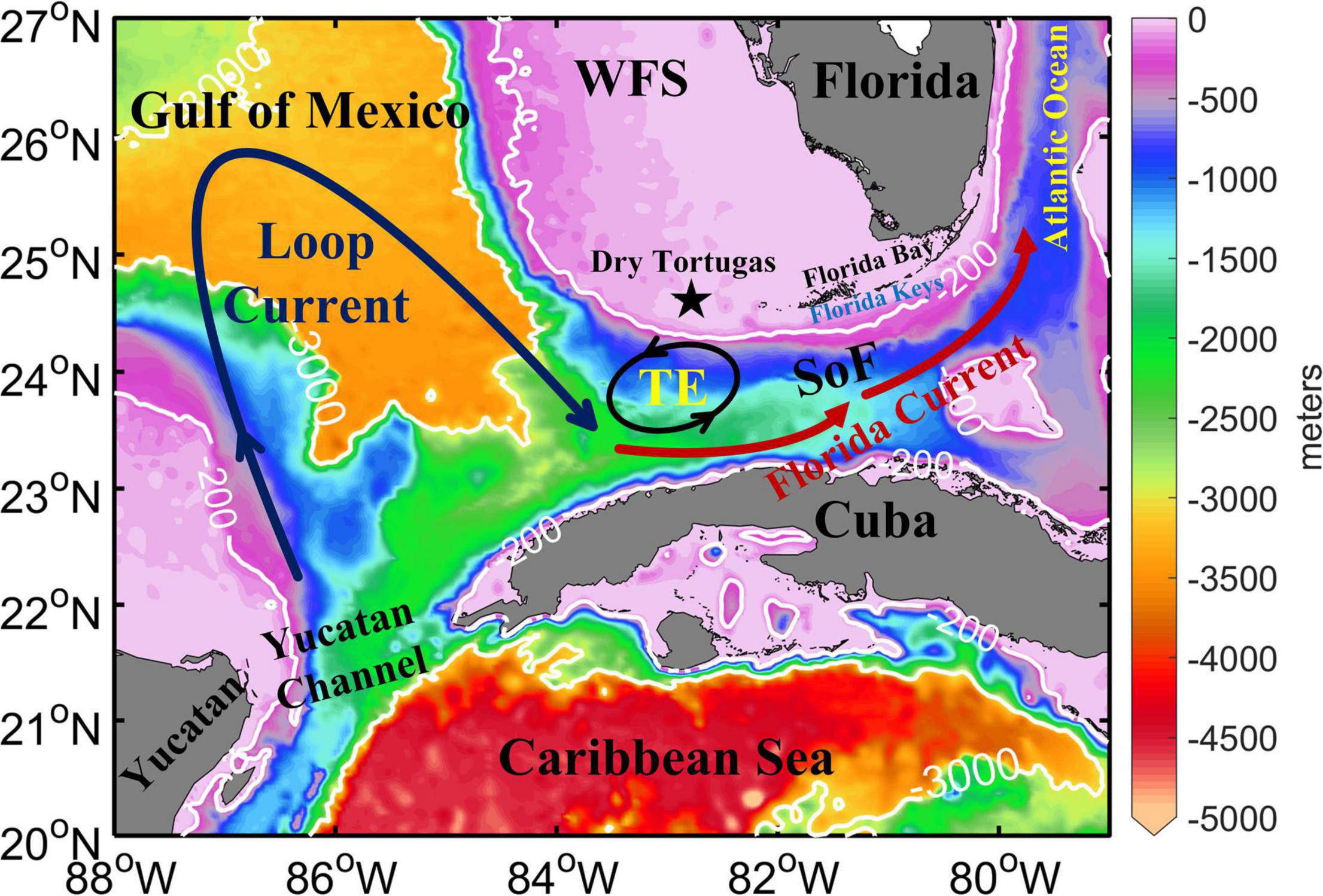
Figure 1. Bathymetry of the southeastern GoM, SoF, and northwestern Caribbean Sea. The 200 and 3,000 m isobaths are annotated with white lines, and the LC and FC are annotated with dark blue and red curves with arrows, respectively. Important bathymetric or geographic features are also noted: the GoM, WFS, SoF, Florida Keys, Florida Bay, Atlantic Ocean, Caribbean Sea, and the Yucatan Channel (YC). The location of the DT is marked with a black pentagram. The black closed circle near the DT indicates the regular location of TEs when they keep quasi-stationary off the DT.

Both submesoscale (<the internal deformation radius of ∼30 km for the SoF, Parks et al., 2009; Kourafalou and Kang, 2012; Zhang et al., 2019) and mesoscale CEs in the SoF are known to be highly productive, providing enhanced food supply for fish larvae (Lee et al., 1994). Those CEs play crucial roles in the transportation of heat, salt, and nutrients, and they contribute to the water exchange between coastal waters and offshore waters (Bulhoes de Morais, 2010). CEs in the SoF also play an important role in the transport, retention, and successful recruitment of larvae of locally spawned grouper and snapper (Lee et al., 1994), juvenile pink shrimp (Criales and Lee, 1996), sailfish (Richardson et al., 2009), spiny lobster (Yeung and Lee, 2002), sea urchin (Feehan et al., 2019), and reef fish (Limouzy-Paris et al., 1997; Porch, 1998; Sponaugle et al., 2005; Shulzitski et al., 2015, 2016, 2017; Vaz et al., 2016). The presence of TEs also corresponds with the period of releasing the LC from contacting or “anchoring” at the “pressure point” of the West Florida Shelf (WFS), and may affect the ecosystems on the shelf (Liu et al., 2016; Weisberg and Liu, 2017).

In addition to the biological and ecological relevance, the CEs in the SoF have been studied in their physical characteristics (e.g., Chew, 1974; Vukovich, 1988; Lee et al., 1992, 1994, 1995; Shay et al., 1998, 2000; Hitchcock et al., 2005; Parks et al., 2009; Chérubin et al., 2021), statistical characteristics (Zhang et al., 2019), and their relationship with the LC perturbations (e.g., Fratantoni et al., 1998) and the FC meandering (e.g., Lee et al., 1994; Kourafalou and Kang, 2012). Recently, the complex current dynamics in the SoF were explored using high frequency radar, satellite altimetry data, and numerical model output (Liu et al., 2021). Some of these previous studies used some SST satellite imagery or ocean current observations from moored instruments (e.g., current meters) to characterize the physical characteristics of TEs, yet it is possible that the studies may not have followed a single TE. This is because TEs can be frequently transformed and/or replenished (Kourafalou and Kang, 2012).

To our knowledge, no study has used continuous observational or modeled data to analyze the entire evolution of CEs in the SoF. Likewise, no study has analyzed the temporal dynamics (e.g., the continuous change of eddy kinetic and potential energy) of CEs during their evolution in the SoF. More importantly, no study has explored the mechanisms contributing to the growth and evolution of CEs in the SoF from the perspective of energy transfer due to the interactions between CEs and the mean flow (the LC/FC system).

The main goal of this study is to understand the physical and biochemical characteristics, physical and kinematic dynamics, and biological implications of a long-lasting CE in the LC/FC system, as well as its interaction with the LC/FC system. This is accomplished through a comprehensive analysis of its 3-dimensional (3-D) structure based on in situ measurements, remote sensing observations, simulations from the global Hybrid Coordinate Ocean Model (HYCOM), and through investigating the continuous variation of eddy energy and exploring the mechanisms that contribute to the growth and evolution of the long-lasting CE.

Data and Methods

Observational Data

Argo Profiling Float Data

Argo float data (Argo, 2000) were downloaded from the Global Argo Data Repository.¹ The data were collected and made freely available by the International Argo Program and the national programs that contribute to it (see text footnote 1),² and were calibrated and validated with the most up-to-date global climatology by the data assembly center (Laxenaire et al., 2019). Data collected by an Argo profiling float (No. D4901061) that located on the edge of the observed CE on June 2, 13 and 23, 2017 are used to examine the vertical temperature and salinity profiles at the eddy boundary, and to evaluate the temperature and salinity profiles extracted from global HYCOM simulations on the same dates for the same locations.

Shipborne Current Measurements

Underway current velocity profiles along ∼82.8^°W between 23 and 24.8^°N were collected by a 300 kHz Teledyne RD Instruments’ (RDI) acoustic Doppler current profiler (ADCP) mounted on the Research Vessel (R/V) Weatherbird II³ over May 24–25, 2017 during an oceanographic cruise (May 13–25, 2017). The observed current data are limited to the layer of ∼5–60 m. The horizontal and vertical structure of the observed current are examined along a transect that right went through the observed CE, and the current data vertically averaged over the layer of ∼5–10 m are used to verify surface current patterns from altimetry measurements and global HYCOM simulations. Details about how the ADCP data were processed and calibrated can be found in Firing and Hummon (2010).

Drifters

The trajectory data of a satellite-tracked drifter (No. 62283) from January 23 to April 22, 2007 obtained from the NOAA Global Drifter Program (GDP) database⁴ are used to reveal a historical CE in the SoF. These data were quality controlled by the Drifter Data Assembly Center (DAC) at the Atlantic Oceanographic and Meteorological Laboratory (AOML), and were interpolated to 6-h intervals through an optimum interpolation procedure called ‘‘kriging.’’⁵

Satellite Observations

Four types of satellite data were used in the analysis. The daily 1 km SST data collected by the Moderate Resolution Imaging Spectroradiometer (MODIS) onboard the Aqua and Terra satellites were downloaded from the NASA Goddard Space Flight Center.⁶ Because the GoM and SoF become nearly isothermal and make it difficult to use SST imagery to detect eddies and fronts during summer months (e.g., Liu et al., 2011a; Zhang and Hu, 2021), only two MODIS SST snapshots on May 9th and 10th, 2017 are used to reveal the eddy signal on SST imagery. Daily 1 km MODIS/Aqua (MODIS/A) Chl data products from April 9 to August 12, 2017 were derived through using the methods described in Hu (2011) and Chen et al. (2019). These data products are generally immune to perturbations by sun glint, thin clouds, stray light, and sensor saturation, thus providing significantly improved coverage over the standard Chl data products in both space and time as shown in Chen et al. (2019) and Zhang et al. (2019). The daily 0.25° × 0.25° altimetry geostrophic velocity data under the product identifier ‘‘SEALEVEL_GLO_PHY_L4_REP_OBSERVATIONS_008_047’’ were processed and distributed by the Copernicus Marine Environment Monitoring Service (CMEMS).⁷ The data products include data collected by multiple altimeter missions, including Cryosat-2, HY-2A, Jason-3, Sentinel-3A, Sentinel-3B, and Saral/AltiKa (see text footnote 7). Data spanning from April 9 to August 12, 2017 are used in this study. The daily 0.25° × 0.25° wind data were taken from the V2.0 Cross-Calibrated Multi-Platform (CCMP) gridded surface vector wind products.⁸ A variational analysis method (VAM) was applied to the version-7 wind data from Remote Sensing Systems (RSS) radiometer, wind vectors from the Quick Scatterometer (QuikSCAT) and Advanced Scatterometer (ASCAT), and wind data from moored buoys as well as ERA-Interim model wind fields to produce these gridded data products. Wind data covering the period of April 9 to August 12, 2017 are used here to explore the potential impact of local wind forcing on the growth and evolution of the observed CE.

Global Hybrid Coordinate Ocean Model Simulations

The 1/12^° global HYCOM (Chassignet et al., 2009; Metzger et al., 2014)⁹ is an operational (real-time forecasts), eddy-resolving model that assimilates various observational data, such as satellite altimetry observations, in situ and satellite SST measurements, and vertical profiles of temperature and salinity from Argo profiling floats, expendable bathythermographs (XBTs), and moored buoys (Cummings, 2005; Putman et al., 2018), thus it maintains the structures of the LC and LC eddies (Weisberg et al., 2011). The global HYCOM performs reasonably well in simulating and resolving major oceanographic features, such as mesoscale eddies, filaments, and fronts (Chassignet et al., 2007; Putman and He, 2013; Putman et al., 2018; Martínez et al., 2019), and shows good agreement with vertical temperature and salinity profiles from in-situ CTD measurements (Cleveland, 2018). The model has been extensively used in many previous studies, including the studies about the Deepwater Horizon oil spill event (Liu et al., 2011b,c; Weisberg et al., 2011, 2017), the oil spill simulations and tracking beyond the GoM (Sun et al., 2018; Paris et al., 2020), the analysis of seasonal and annual variations in the dispersal of post-hatching sea turtles (DuBois et al., 2020), the prediction of annual variations in the distribution and abundance of juvenile sea turtles in the northwestern Atlantic Ocean (Putman et al., 2020a), the dynamics of sediments in the northern GoM (Zang et al., 2019), the heat content estimation for the GoM (Luo et al., 2015), the studies about pelagic Sargassum (Hu et al., 2016; Brooks et al., 2018; Putman et al., 2018, 2020b; Shadle et al., 2019; Johns et al., 2020), the retention and dispersion of virtual fish larvae (Martínez et al., 2020), the characterization of larval swordfish habitat (Suca et al., 2018), and the upper ocean response to typhoons (Wu and Li, 2018). The global HYCOM has been used for boundary conditions in coastal and regional models of higher resolution, as in the Gulf of Mexico at 1/25° and 1/50° (Mezić et al., 2010; Le Hénaff et al., 2012; Le Hénaff and Kourafalou, 2016; Kourafalou et al., 2018).

In order to investigate the physical and biochemical characteristics, as well as the 3-D structure of the long-lasting CE, we used simulated ocean current, temperature, and salinity data from the global HYCOM. The simulated data were also used to analyze the changes of eddy kinetic and potential energy over time, and to perform energy transfer analysis in order to identify the mechanisms that contributed to the evolution and growth of the CE. Current velocity, temperature, and salinity data spanning from April to August 2017 were taken from the global HYCOM experiment 92.8 (data are available for 02/01/2017-05/31/2017)¹⁰ and experiment 57.7 (data are available for 06/01/2017 to 09/30/2017).¹¹ Surface current data during 2010--2015, extracted from the global HYCOM reanalysis dataset (experiment 53.x)¹² were used to analyze the long-term occurrence frequency of the CEs in the southeastern GoM and SoF. These experiments provide data every 3 h for 40 layers extending from the ocean surface to 5,000 m. The sill depth of the SoF is around 800 m, which limits the depth of the FC and dynamics of the upper layer (Furey et al., 2018; Hamilton et al., 2018, 2019). Thus, global HYCOM simulations on the top 31 layers (0–800 m) are used in this study. The data in 3-h temporal resolution are averaged to daily files through daily average.

Evaluation of the Global Hybrid Coordinate Ocean Model in the Study Area

The global HYCOM is one of the state-of-the-art community global models (Dombrowsky et al., 2009) and is run at the Naval Research Lab – Stennis Space Center (NRL-SSC), where validation exercises are routinely performed for model evaluation and continuous improvements (e.g., Metzger et al., 2008, 2017); indirect model evaluation is also performed through evaluation of nested models that use global HYCOM for boundary conditions. However, the accuracy of global HYCOM simulations in the study area has not been explored. Qualitative evaluation in the SoF shows that the global HYCOM can simulate the long-lasting CE and reproduce the same evolution process as observed by altimeters and ocean color satellites. Such a capacity is important for the objectives of this study. To further evaluate global HYCOM simulations, we used observational data to compare both surface and subsurface data from the global HYCOM. Specifically, surface current patterns from the global HYCOM were compared with altimetry surface current patterns to see if they agreed well, and both current patterns were overlaid on the corresponding MODIS/A Chl images to support biological implications from the CE. In addition, we also used ADCP-based current data to evaluate global HYCOM surface current data. For the evaluation of global HYCOM subsurface data, vertical salinity and temperature profiles collected by an Argo profiling float on June 2, 13 and 23, 2017 were used to compare with those from global HYCOM simulations.

Methods

Several different algorithms have been proposed to automatically detect and track eddies from either current velocity fields or sea surface height (SSH) maps. Of these, some are based on physical parameters (e.g., Chelton et al., 2007) or geometrical properties such as closed streamlines or SSH contours (e.g., Sadarjoen and Post, 2000; Chaigneau et al., 2008, 2009; Nencioli et al., 2010; Chelton et al., 2011; Faghmous et al., 2015), while others involve both physical parameters and geometrical properties (e.g., Kang and Curchitser, 2013; Halo et al., 2014; Le Vu et al., 2018). The algorithms based on dynamic physical parameters may exclude weak eddies, and are sensitive to the thresholds selected for determining eddy boundaries, while algorithms based on geometrical properties are sensitive to both weak and intense eddies (Le Vu et al., 2018). In this study, the Angular Momentum Eddy Detection Algorithm (AMEDA, Le Vu et al., 2018) is selected and applied to surface current velocity fields from both altimetry measurements and global HYCOM simulations to detect and track the long-lasting CE. This algorithm is hybrid to combine the geometrical properties of velocity fields (closed streamlines) and a dynamic physical parameter (local normalized angular momentum, LNAM). It can be applied to various velocity fields with different spatial resolutions without the need of fine-tuning parameters. The algorithm can also identify eddy splitting and merging, thus helping to explore eddy-eddy interactions and to accurately identify the formation areas of long-lived eddies. These are the main advantages of the AMEDA algorithm, and this algorithm has been used widely in many studies on ocean eddies (e.g., Ioannou et al., 2017; de Marez et al., 2019, 2020; Morvan et al., 2020; Zhu and Liang, 2020; Pegliasco et al., 2021; Stegner et al., 2021).

In the AMEDA algorithm, the eddy center is defined as the location corresponding to an extremum of the LNAM, and the eddy boundary is defined as the outermost closed streamline around the eddy center. The eddy radius is computed as the equivalent radius of a circle with the same area as the one bounded by the eddy boundary (Ioannou et al., 2017; Le Vu et al., 2018; Morvan et al., 2020). The similarity in shapes and the spatial closeness between successively detected eddies is utilized to perform eddy tracking. Full description about the AMEDA algorithm can be found in Le Vu et al. (2018). For eddy detection based on altimetry measurements, the original current velocity data (1/4^° × 1/4^°) were linearly interpolated into a 1/8^° × 1/8^° degree grid to enhance the performance of eddy detection, this method was also used in Liu et al. (2012) and Sun et al. (2019). To analyze eddy kinematic properties, the relative vorticity (ζ) of the flow and the Okubu-Weiss (OW) parameter (Okubo, 1970; Weiss, 1991) that quantifies the relative importance between local deformation and rotation are calculated from global HYCOM simulations as follows:

$\mathrm{\zeta }=\partial v/\partial x-\partial u/\partial y(1)$

$OW=S_n^2+S_s^2-{\mathrm{\zeta }}^2(2)$

Where S_n = (∂⁡u/∂⁡x)−(∂⁡v/∂⁡y), S_s = (∂⁡v/∂⁡x) + (∂⁡u/∂⁡y) denote the normal strain component (e.g., stretching deformation) and shear strain component (e.g., shearing deformation), respectively. Here, u and vare the zonal and meridional components of the current velocity. The current velocity field within an eddy is typically rotation dominated, thus the eddy interior is generally characterized by negative values of OW parameter.

Conceptually, positive wind stress curl produces divergence at the surface water and causes upwelling, while negative wind stress curl produces convergence at the surface water and induces downwelling (Hwang and Chen, 2000). Subsurface cold waters are brought to the surface layer by upwelling which can form cold-core eddies, while downwelling deepens the thermocline and can lead to the formation of warm-core eddies. Wang et al. (2008) suggests that wind stress curls related to wind jets could be a significant formation mechanism of the extensive eddy activity in the South China Sea (SCS). Here, we also explore the effect of wind stress curl on the generation and evolution of the observed CE. The wind stress curl is calculated as:

$Curl\overrightarrow{\mathrm{\tau }}=\frac{\partial {\mathrm{\tau }}_y}{\partial x}-\frac{\partial {\mathrm{\tau }}_x}{\partial y}(3)$

Where τ_y = ρC_Du_y|u|, τ_x = ρC_Du_x|u| are meridional and zonal components of the wind stress. ρ denotes the air density at the sea surface. C_D is the drag coefficient computed using the quadratic formulation (Large et al., 1994): 10³C_D = 2.70/|u| + 0.142 + 0.0764|u|. $\overrightarrow{u}=(u_x,u_y)$ represent the wind velocity at 10 m above the sea surface and |u| is the wind speed.

The barotropic and baroclinic instability induced by the mean flow have been demonstrated to play an important role in the generation and evolution of eddies in extensive studies (e.g., Zu et al., 2013; Donohue et al., 2016; Li et al., 2016; Qian et al., 2018; Zhao et al., 2018; Mandal et al., 2019; Tedesco et al., 2019; Yang et al., 2020). Yang et al. (2020) examined the instability and multiscale interactions underlying the LC eddy shedding based on the ensembles of flow fields output from a numerical model. To check if the LC/FC system induced barotropic and baroclinic instability are potential mechanisms that contribute to the growth and evolution of the observed CE as well as the modulation of eddy energy, we utilized the global HYCOM simulations to calculate eddy energy and investigate the potential and kinetic energy transfer between the LC/FC system and the CE. Following Oey (2008), Zhan et al. (2016), and Luecke et al. (2017), the eddy kinetic energy (EKE), eddy potential energy (EPE) and energy conversion terms (BT and BC) are defined as follows:

$\text{EKE =} \frac{1}{2} \left(\overline{u^{{\prime }^2}}+\overline{v^{{\prime }^2}}\right)(4)$

$\text{EPE}=\frac{g^2}{2\overline{N^2}}\frac{\overline{{\rho }^{{\prime }^2}}}{{\rho }_0^2}(5)$

$\text{BT}=-\left(\overline{u^{{\prime }^2}}\frac{\partial \overline{u}}{\partial x}+\overline{v^{{\prime }^2}}\frac{\partial \overline{v}}{\partial y}+\overline{u^{\prime }{v}^{\prime }}\frac{\partial \overline{u}}{\partial y}+\overline{u^{\prime }{v}^{\prime }}\frac{\partial \overline{v}}{\partial x}\right)(6)$

$\text{BC}=-\frac{g^2}{{\mathrm{\rho }}_0^2\overline{N^2}}\left(\overline{u^{\prime }{\mathrm{\rho }}^{\prime }}\frac{\partial \overline{\mathrm{\rho }}}{\partial x}+\overline{v^{\prime }{\mathrm{\rho }}^{\prime }}\frac{\partial \overline{\mathrm{\rho }}}{\partial y}\right)(7)$

Where the overbar represents time average, and the prime denotes the deviation from the mean state that averaged from April to August 2017. u, v, ρ, g are the zonal and meridional current velocities, sea water density, and the gravitational acceleration, respectively. ρ′(x,y,z,t) = ρ(x,y,z,t)−ρ_b(z), where ρ_b(z) is a depth-dependent background density that calculated as the horizontal and temporal mean over the study region from April to August 2017. ρ₀ = 1025 kg/m³ is the reference seawater density. N² denotes the squared buoyancy frequency and is given by N² = −(g/ρ₀)∂⁡ρ/∂⁡z. BT denotes the energy transfer due to the work of the Reynolds stress against the mean shear (Eden and Böning, 2002). Positive BT indicates that the mean kinetic energy is converted to EKE through barotropic instability. BC represents the conversion between the mean potential energy and EPE, and positive BC implies that the mean potential energy is converted to EPE through baroclinic instability.

Results

Evaluation of the Global Hybrid Coordinate Ocean Model in the Study Area

Figure 2 shows the comparison results between altimetry surface currents and global HYCOM surface currents. The patterns of the LC and LC frontal eddies (denoted by thick red arrows in Figures 2A–F), as well as the CE off the DT (denoted by thick magenta arrows in Figures 2A–H) appear similar between altimetry and global HYCOM, suggesting validity of the model simulations. Both altimetry and model-derived surface current distributions (Figures 2A–H) are in agreement with the MODIS/A Chl features (color codes in Figures 2A–H). Both altimetry and model-derived current patterns also agree well with the ADCP-based current observations. Specifically, the currents vertically averaged over the layer of ∼5–10 m (thin magenta vectors in Figures 2I,J), measured by a shipborne ADCP during May 24–25 are consistent with altimetry (Figure 2I) and model (Figure 2J) derived mean surface current patterns from April 23 to July 15, when the CE was quasi-stationary off the DT. In addition, the mean root-mean-square deviation (RMSD) between the zonal current velocities along the ship’s track (Figures 2I,J) from the ADCP and global HYCOM is 0.152 m/s, and the mean RMSD of the meridional current velocities between them is only 0.039 m/s. Vertical temperature and salinity profiles collected by an Argo profiling float (location shown as black pentagrams in Figure 3, left column) on June 2, June 13, and June 23, 2017 were found in good agreement with model-simulated vertical temperature and salinity profiles (Figure 3, middle and right columns). The RMSDs between vertical temperature profiles from the Argo profiling float and global HYCOM on June 2, June 13, and June 23, 2017 are 0.107, 0.344, and 0.502^°C, respectively. The RMSDs of vertical salinity profiles between them on June 2, 13, and 23, 2017 are 0.014, 0.025, and 0.014 psu, respectively. Thus, the consistency between global HYCOM simulations and all other observational data in the study area suggests that it is appropriate to use global HYCOM archives to study the 3-D structure of the long-lasting CE and to explore the interaction between the CE and the LC/FC system.

FIGURE 2

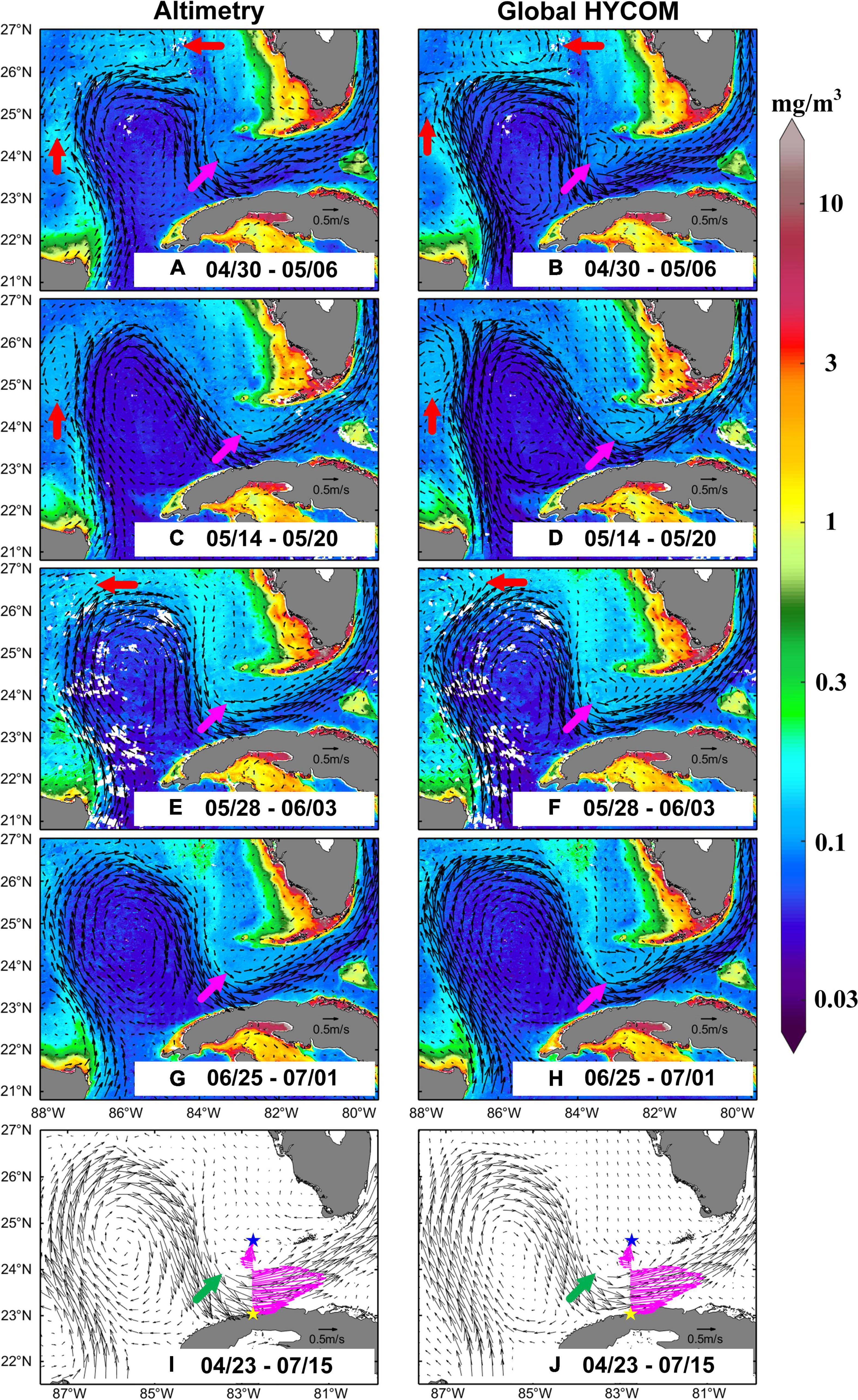
Figure 2. Comparison of surface current distributions from altimetry observations (left column) and global HYCOM simulations (right column). The color codes in (A–H) indicate MODIS/A Chl distributions. The location of the CE off the DT is annotated with a thick magenta and green arrow in (A–H) and (I,J), respectively. The locations of several LC frontal eddies are annotated with thick red arrows in (A–F). The currents (thin magenta vectors, vertically averaged over the layer of ∼5–10 m) measured by shipborne ADCP on May 24 and 25, 2017 are overlaid in (I,J) for altimetry and global HYCOM, respectively. The yellow and blue pentagrams in (I,J) denote the start and end points of the ship’s track.

FIGURE 3

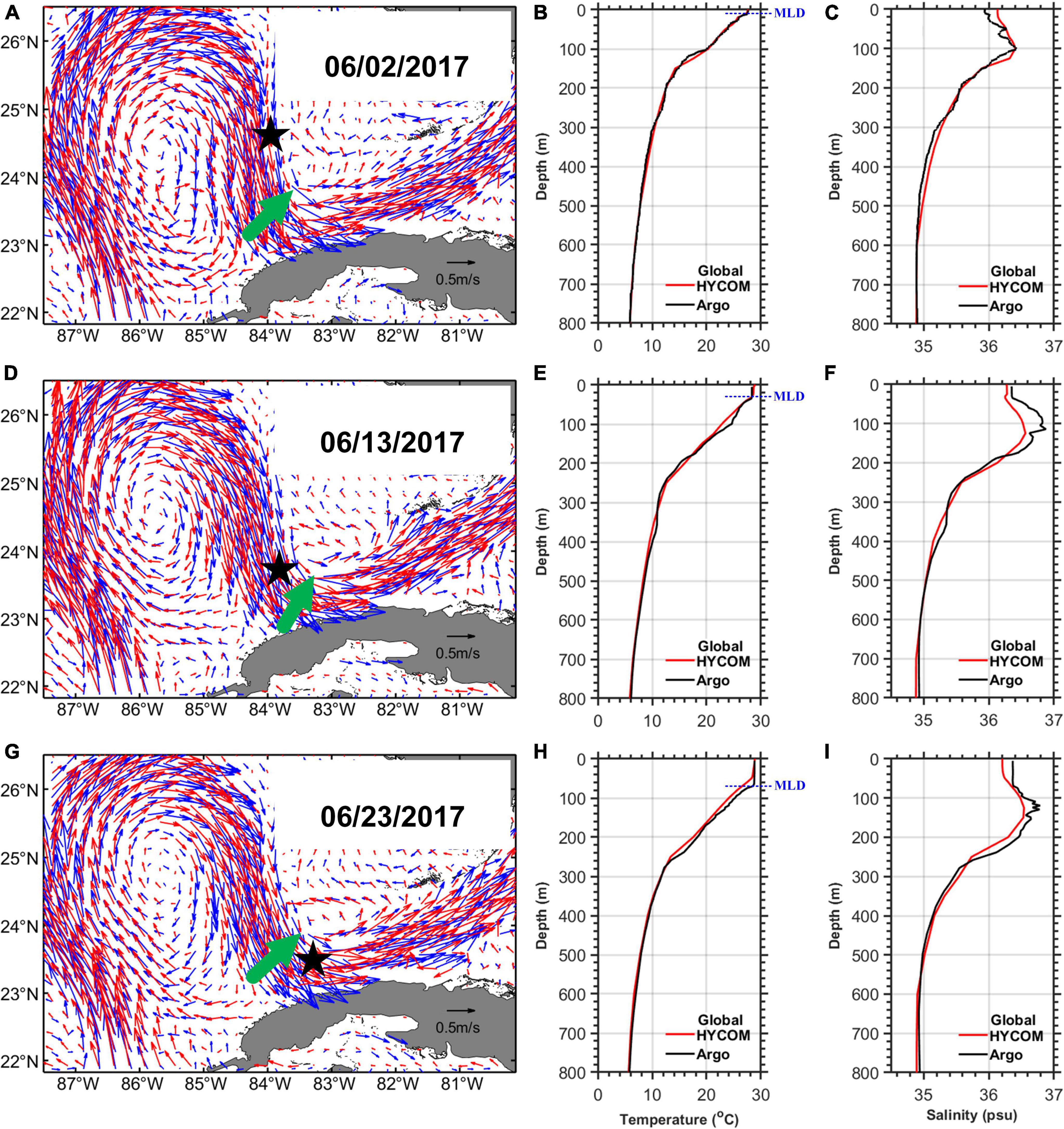
Figure 3. Comparison of surface current distributions (left column; A,D,G) from altimetry observations (blue vectors) and global HYCOM simulations (red vectors), and comparison of subsurface temperature (middle column; B,E,H; unit: °C) and salinity (right column; C,F,I; unit: psu) profiles from an Argo profiling float (black color) and global HYCOM simulations (red color) on June 2, 13, and 23, 2017. In the left column, the location of the CE off the DT is annotated with thick green arrows, and the location of the Argo profiling float located on the edge of the CE is annotated with black pentagrams. The MLDs estimated from the temperature profiles collected by the Argo profiling float are denoted by dashed blue lines in the middle column.

Eddy Surface Characteristics

The mesoscale CE (arrows in Figure 4) off the DT is captured in Chl and SST images, as indicated by the higher Chl and lower temperature than surrounding waters. The AMEDA algorithm was applied to daily altimetry geostrophic velocity data from April to August, 2017 to detect and track the CE. The results indicate that the CE was detected as a frontal eddy along the eastern edge of the LC on April 9th, 2017. Continuous weekly MODIS/A Chl and weekly global HYCOM surface current distributions (Figure 5) reveal how the CE evolved from April 9 to August 12, 2017, where the CE was carried to the DT by the LC, and then remained quasi-stationary off the DT from around April 23 to July 15, 2017, after which it propagated eastward when a larger LC frontal eddy (denoted by white arrows in Figures 5N–R) was approaching. The evolution process of the simulated CE shown in Figure 5 is indeed similar to the evolution process captured by altimetry observations (shown in Supplementary Figure 1). Because the CE stayed for a long time (around 3 months) off the DT during its evolution, we name it a TE. Each panel in Figure 5 corresponds to a phase during the evolution of the TE. Therefore, the life cycle of this TE consists of 18 phases. In Figure 5, the LC features from global HYCOM simulations match very well with the MODIS/A Chl patterns during all phases, while the Chl features within the TE are only in good agreement with the model-simulated surface current patterns during phases 1–14 (Figures 5A–N, April 9 to July 15, 2017). This is because when the TE moved eastward along the Florida Keys after phase 14 (Figure 5N), it was getting closer to the coasts and became smaller due to the interaction with the topography and the FC (e.g., getting absorbed into a meander of the FC), which could not be resolved well by the 1/12^° model fields. In addition, nearshore altimetry data assimilated in global HYCOM contain large uncertainties.

FIGURE 4

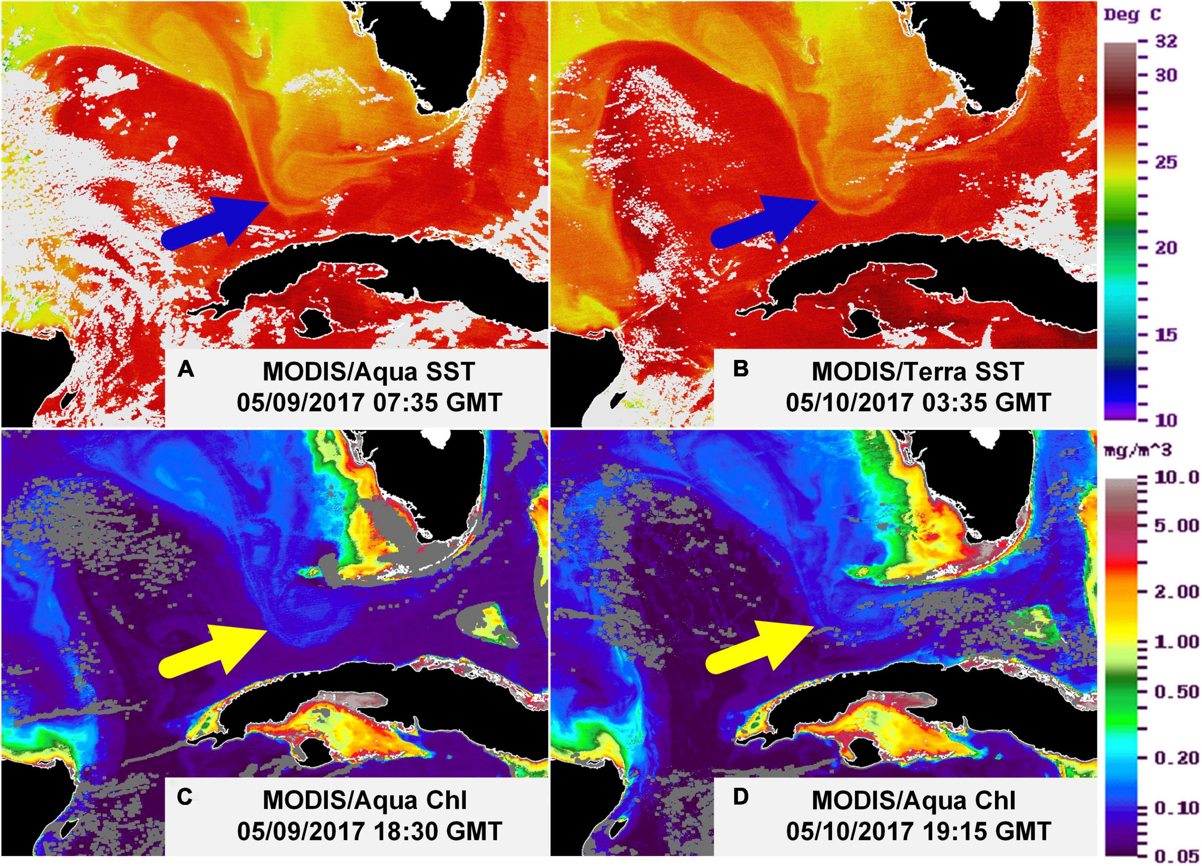
Figure 4. MODIS SST (A,B) and Chl (C,D) imagery on May 9 and 10, 2017 showing a CE off the DT, which is annotated with blue and yellow arrows. The images cover a region of 20–27°N and 88–79°W. The white color in the SST imagery and the gray color in the Chl imagery indicate no data.

FIGURE 5

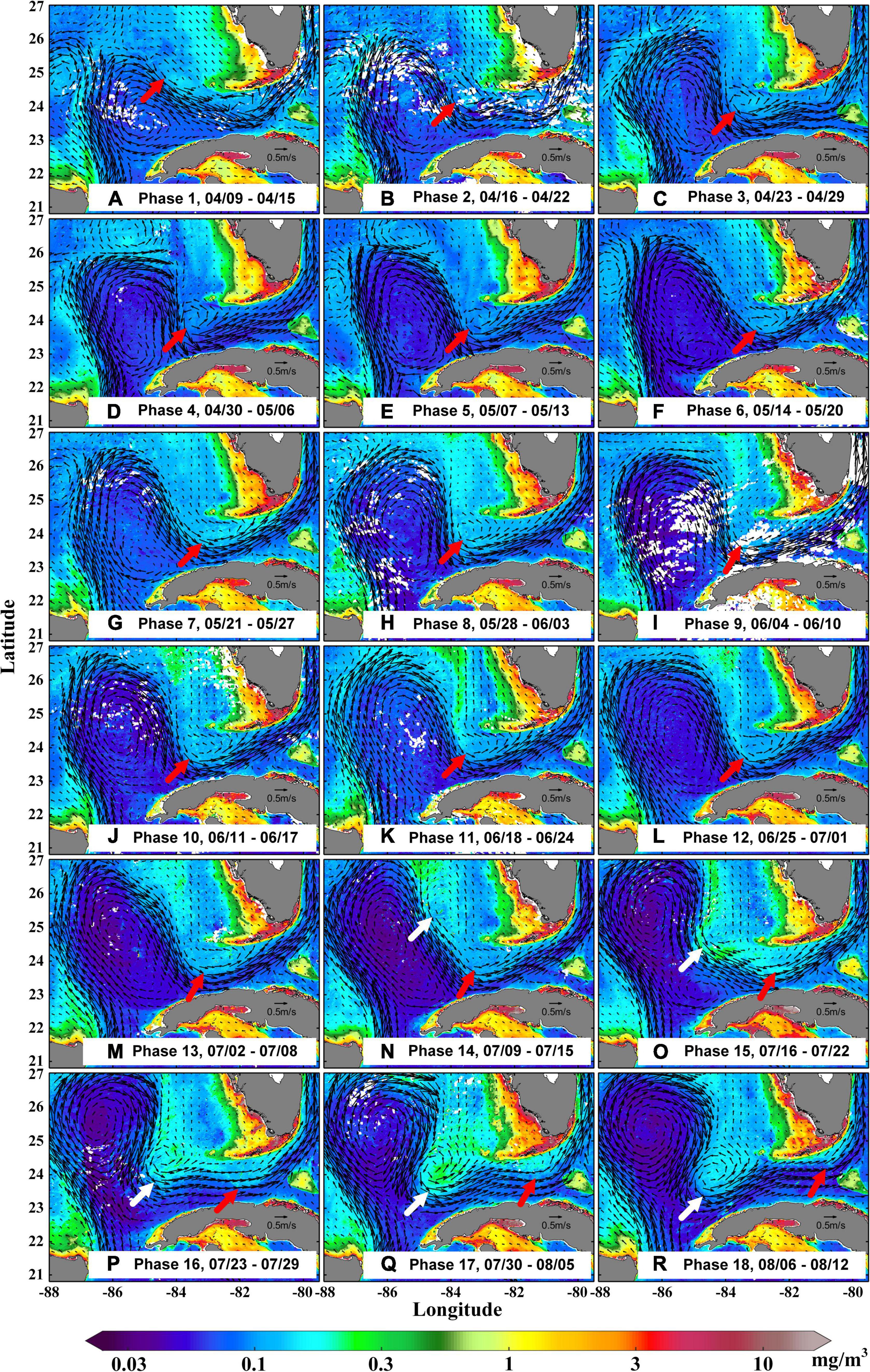
Figure 5. Sequential weekly MODIS/A Chl imagery with weekly global HYCOM simulated surface currents (black vectors, with scales overlaid on land) overlaid from 04/09/2017 to 08/12/2017, showing the entire evolution of a model-simulated CE annotated with a thick red arrow in each image (A–R). White color means no data, and thick white arrows denote a new LC frontal eddy in (N–R).

Figure 6 shows the mean model-simulated surface current patterns during phases 3–14 (April 23 to July 15, 2017) when the TE stayed quasi-stationary off the DT. As shown in Figure 6A, both model-based current simulations and ADCP-based current observations show relatively weak currents (< 0.5 m/s) in the northern part of the TE and stronger currents (> 0.5 m/s) in the southern part. The eddy centers, as determined by the AMEDA algorithm based on the surface currents from model simulations during phases 1–14 (Figures 5A–N, April 9 to July 15, 2017) are shown in Figure 6B, where the center locations are color coded. During phases 1–14 (April 9 to July 15, 2017), the mean TE radius was determined to be 48.4 km from altimetry and 51.6 km from global HYCOM.

FIGURE 6

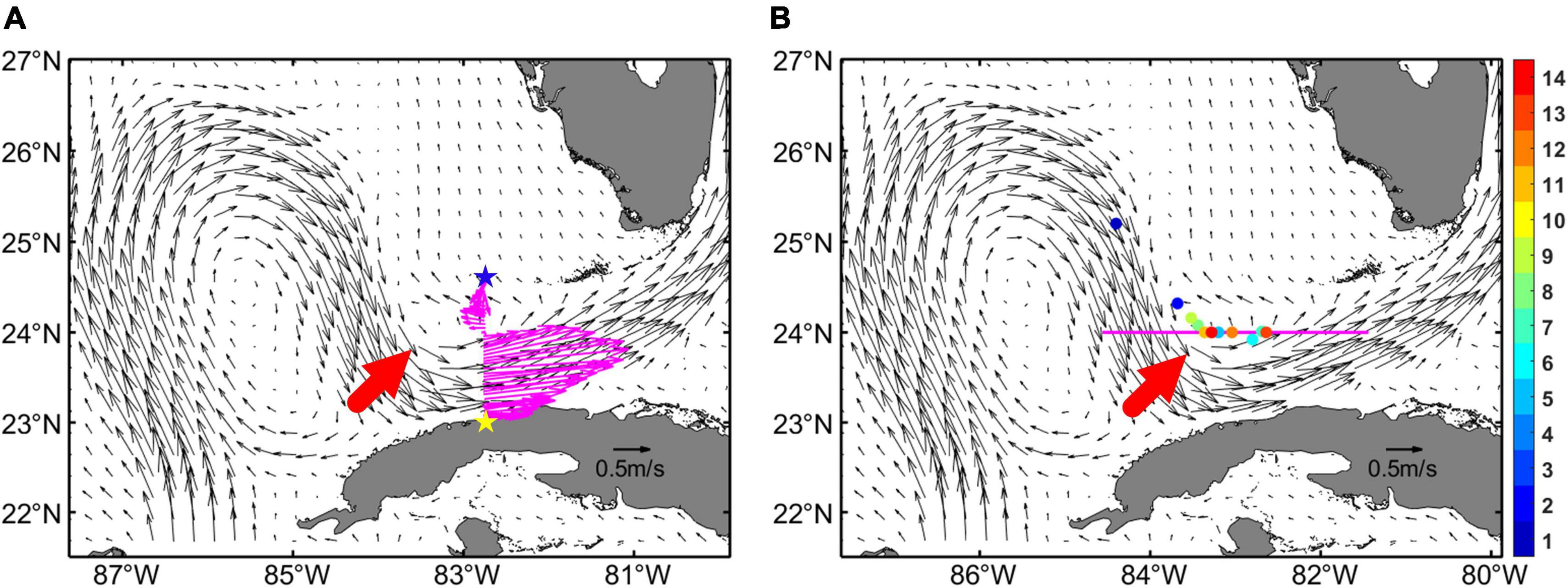
Figure 6. Distribution of mean global HYCOM surface currents (black vectors in A,B) over phases 3–14 (April 23 to July 15, 2017), during which the TE annotated with a thick red arrow was quasi-stationary off the DT. (A) is same to Figure 2J. The ADCP-based currents (vertically averaged over the layer of ∼5–10 m) collected between May 24 and 25, 2017 are overlaid as thin magenta vectors in (A). The yellow and blue pentagrams in (A) denote the start and end points of the ship’s track. The eddy centers are determined by the AMEDA algorithm based on weekly mean model surface current velocities during phases 1–14 (shown in Figure 5, April 9 to July 15, 2017) and are denoted by colored dots in (B), where the time (phase, represented by week number) is color coded. A horizontal section passing through the center of the simulated TE is annotated with magenta color in (B), along which the vertical structures of mean simulated temperature, salinity, density, and the squared buoyancy frequency from April 23 to July 15, 2017 are presented in Figure 9.

Eddy Vertical Structure

The vertical structure of the TE can be visualized in Figure 7, which illustrates the vertical profile of current velocities that are normal to the ship’s track shown in Figure 6A. The warm colors represent eastward currents, while the cold colors indicate westward currents. The fastest eastward currents (∼1.6 m/s) were observed between 23.5 and 23.8^°N, which indicates the main axis of the FC. The velocities of westward currents off the TE region were between 0.1 and 0.4 m/s. The current profiles observed by shipborne ADCP nicely reveal the existence of the TE, but they are only limited to around 60 m, which may not reveal the whole vertical structure of the TE.

FIGURE 7

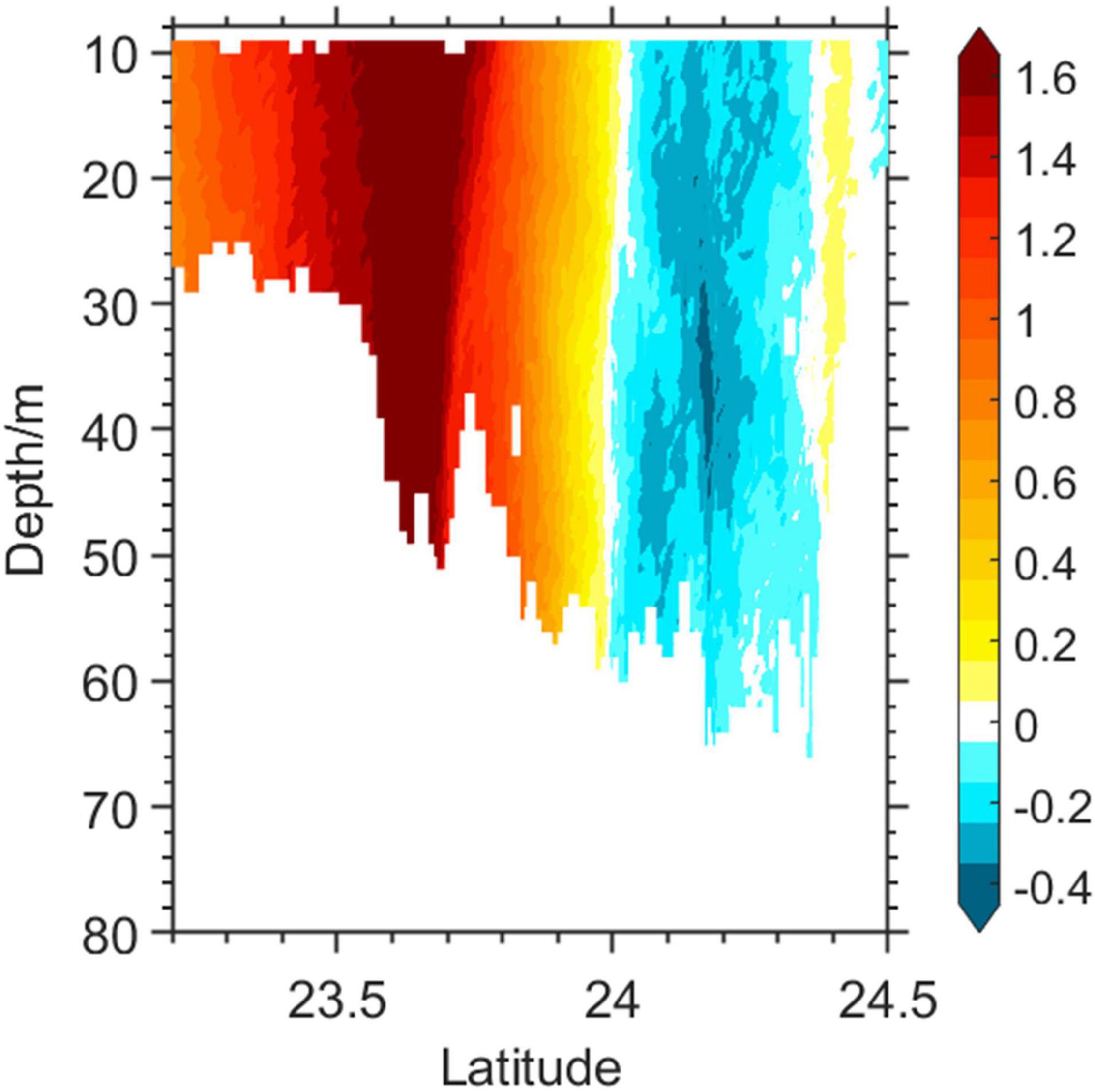
Figure 7. Vertical profile of current velocities (unit: m/s) in directions normal to the ship’s track, measured by the shipborne ADCP during May 24–25, 2017. The ship’s track is annotated in Figures 2I, 2J, 6A. Color scale denotes the current speed, positive to the east and negative to the west.

An Argo profiling float (black pentagrams in Figures 3A,D,G) were found on the edge of the TE on June 2, June 13, and June 23, 2017. The observed temperature and salinity profiles are shown as black lines in the middle and right columns of Figure 3, respectively, together with model simulation results (red lines). Water temperature was around 27–29^°C at surface, and it decreased with depth. The mixed layer depths (MLDs) from the Argo profiling float were around 10, 35, and 70 m for June 2, June 13, and June 23, respectively. Both the Argo profiling float and global HYCOM reveal that the saltiest waters (36.4–36.8 psu) were mainly distributed in the layer of ∼100–140 m.

The distributions of mean water temperature and salinity on the selected six layers (0, 50, 150, 300, 500, and 800 m) from phase 3 to phase 14 (April 23 to July 15, 2017), during which the TE remained quasi-stationary off the DT are shown in Figures 8A,B, respectively. There is no apparent difference in the surface temperature between the TE and the surrounding waters, but subsurface temperature patterns clearly reveal a cold core eddy, where the temperature within the TE is 2–4^°C cooler than in the surrounding waters, a result of upwelling. As shown in Figure 8B, the highest salinity (∼36.4 psu) within the TE is found in the layer of 50 m. For the layers at 150 m, 300 m, and 500 m, the waters in the LC region are around 0.4–0.8 psu saltier than those within the TE. This is also because less salty deep waters were upwelled to upper layers within the TE. Figure 8C shows that the TE is characterized by positive relative vorticity, and the relative vorticity at surface and 50 m depth are around 0.35 times the local Coriolis parameter. As the water depth increases, the ratio between them gradually decreases, reaching ∼0.1 at a depth of 800 m. These results are consistent with results obtained from in situ data for a LC frontal eddy near the SoF in 2016 (Le Hénaff et al., 2020) and from the Regional Ocean Modeling System (ROMS) for the Southern California Bight (Dong et al., 2012) and the SCS (Lin et al., 2015). Negative OW parameter dominates the TE from surface to 800 m as shown in Figure 8D, indicating rotation dominates over strain in the eddy region.

FIGURE 8

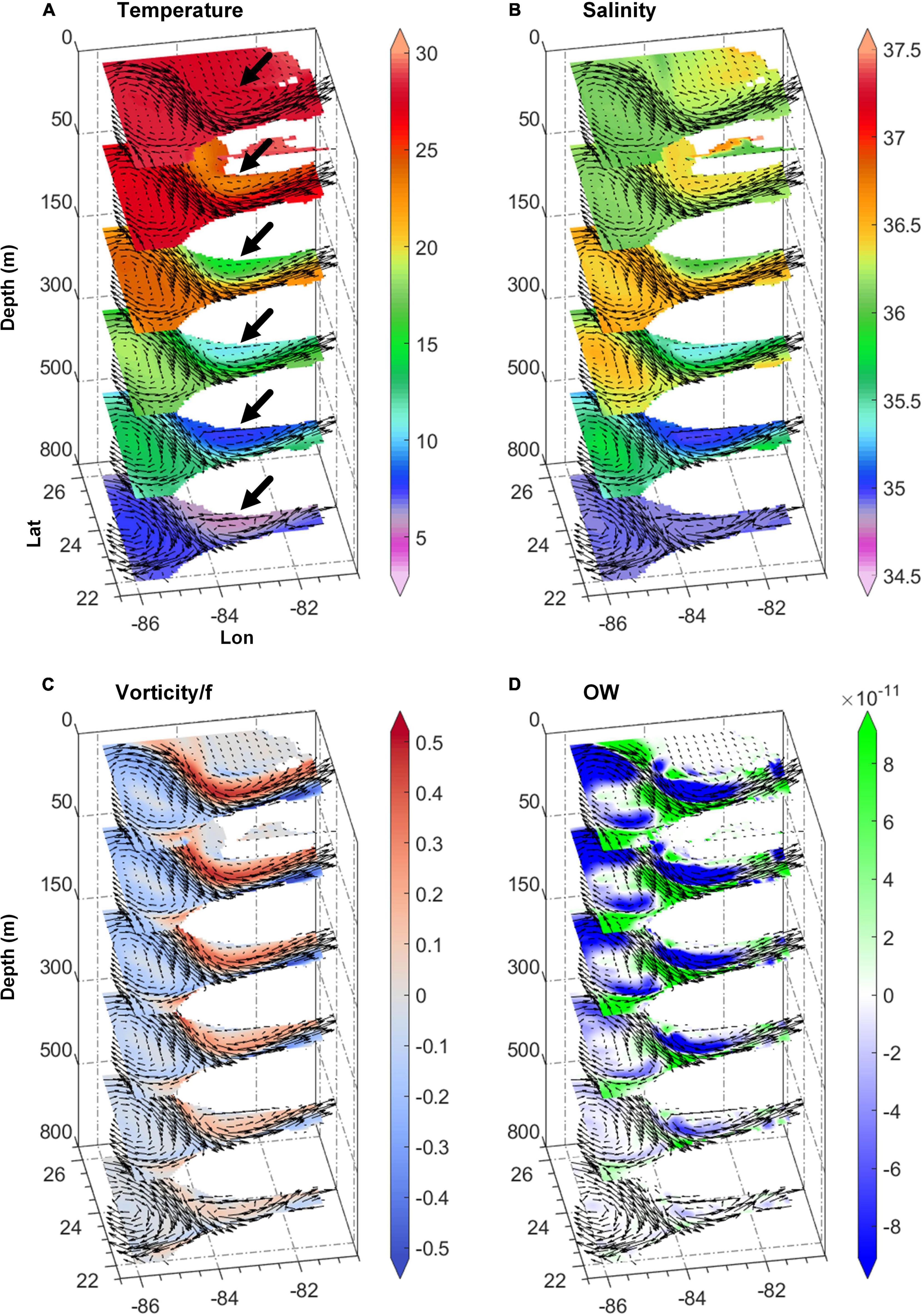
Figure 8. Distributions of mean water temperature (A, unit: ^°C), salinity (B, unit: psu), relative vorticity (C, normalized by the local Coriolis parameter, unitless), and OWparameter (D, unit: s^–2) on the selected six layers. These variables are averaged from April 23 to July 15, 2017, during which the TE remained quasi-stationary off the DT. The mean simulated currents on each layer during the same period are overlaid as black vectors in each figure. The location of the TE on the six layers is annotated with thick black arrows in (A).

The subsurface properties of mean water temperature, salinity, and density during phases 3–14 (April 23 to July 15, 2017) along a zonal section (the magenta line in Figure 6B) passing through the TE are shown in Figures 9A–C. The doming of the isotherms (Figure 9A), isohalines (Figure 9B), and isopycnals (Figure 9C) all indicate upwelling within the TE. The upwelling brought low temperature and low salinity deep waters into the upper layers (Figures 9A,B). The subsurface salinity maximum (>36.4 psu) occurs at 90–160, 60–120, and 80–140 m at the western edge, center, and eastern edge of the TE, respectively (Figure 9B). The doming of the isopycnals between the surface layer (∼40 m) and 800 m (Figure 9C) indicates the deep penetration of the TE up to 800 m. The isotherms, isohalines, and isopycnals all reach their shallowest depths at around 83.4^°W. The vertical profile of the squared buoyancy frequency (N²) along the selected zonal section is shown in Figure 9D. It reveals that water stratification is pronounced within ∼120 m of water depth, and reaches the maximum between 20 and 50 m, indicating that waters in this layer are quite stable and inhibit vertical exchange of heat, salt, and momentum.

FIGURE 9

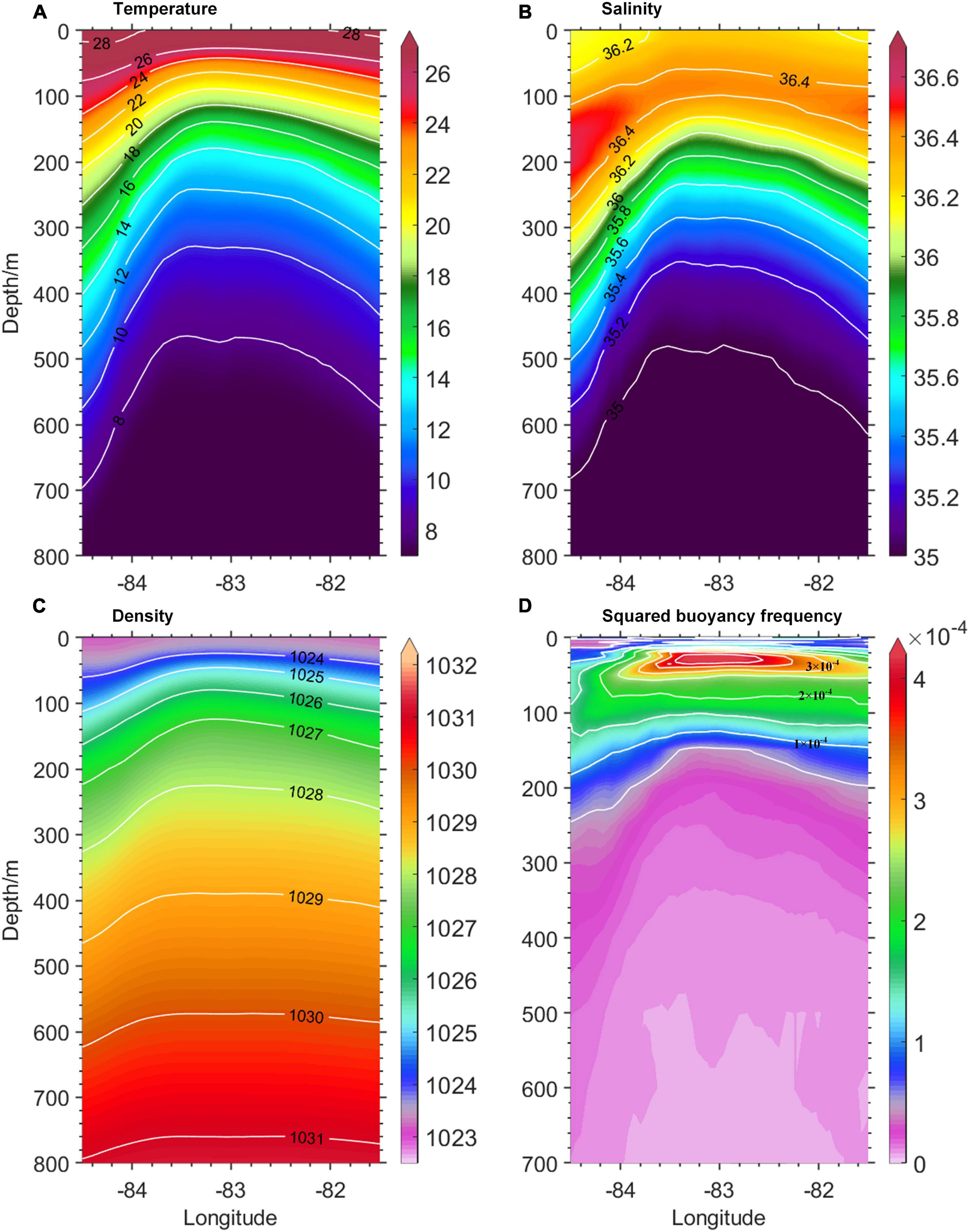
Figure 9. Vertical distributions of mean simulated water temperature (A, unit: ^°C), salinity (B, unit: psu), density (C, unit: kg/m³), and the squared buoyancy frequency (D, unit: s^–2) along a zonal section (annotated with a magenta line in Figure 6B) from April 23 to July 15, 2017, during which the TE remained quasi-stationary off the DT.

Mechanisms Behind the Growth and Evolution of the Tortugas Eddy

The modulations of the LC/FC front can significantly affect the local circulations off the DT, and perturbations of the FC can also influence the generation and evolution of TEs (Kourafalou et al., 2018). An energy transfer analysis, based on global HYCOM simulations, is used to evaluate the contributions of the barotropic and baroclinic instability induced by the LC/FC system to the growth and evolution of the TE. The horizontal distributions of vertical mean EKE and EPE averaged over April 9th to August 12th, 2017 are shown in Figures 10A,B, respectively. Figure 10A shows that the LC region and SoF are the most energetic regions for eddy activities as characterized with large EKE values. Figure 10B shows that the northern edge of the SoF’s entrance is characterized with large EPE values. The eddy centers (black dots in Figures 10A,B) determined from weekly mean model-simulated surface current fields during phases 1–14 (Figures 5A–N, April 9 to July 15, 2017) are all located in high EKE and EPE regions. The horizontal distributions of vertical mean BT and BC averaged from April 9th to August 12th, 2017 are shown in Figures 10C,D, respectively. It is evident that large positive BT and BC are found in the YC and LC region, as well as the entrance of the SoF. This signifies that a large amount of energy of mean flow was transferred to eddies, which is favorable for the generation and growth of eddies. Considering the model-based eddy centers during phases 1–14 (April 9 to July 15, 2017) shown as black dots in Figures 10C,D, we found that the TE came across regions with positive BT and BC during its evolution. This indicates that the TE’s evolution was impacted by both barotropic and baroclinic instability that induced by the LC/FC system. The TE area was found to have high barotropic and baroclinic instability according to an analysis of multi-year model output (Yang et al., 2020). The magnitudes of BT and BC are similar over the LC/FC system, which suggests that both barotropic and baroclinic instability are important for the evolution of the TE. Note that large negative BT and BC are found in the nearshore regions off the Florida Keys, which means that eddy energy was converted to the energy of the FC in those regions. This result is consistent with the fact that mesoscale CEs generally evolve to small (submesoscale) CEs and finally decay along the Florida Keys. Of course, care should be taken in interpreting the details of the BT and BC conversions, because the global HYCOM (which assimilates observational data into the model) is not a free-run model that is required to conserve the total energy of the ocean system (e.g., Yang et al., 2020). However, we note that a similar approach has been taken to diagnose BT/BC conversion in several other studies using data assimilative models (e.g., Qian et al., 2018; Mandal et al., 2019). Energy transfer attributed to ocean dynamics can be separated from that introduced through data assimilation (e.g., Oke and Griffin, 2011; Schiller and Oke, 2015), but that is not pursued here due to lack of relevant data.

FIGURE 10

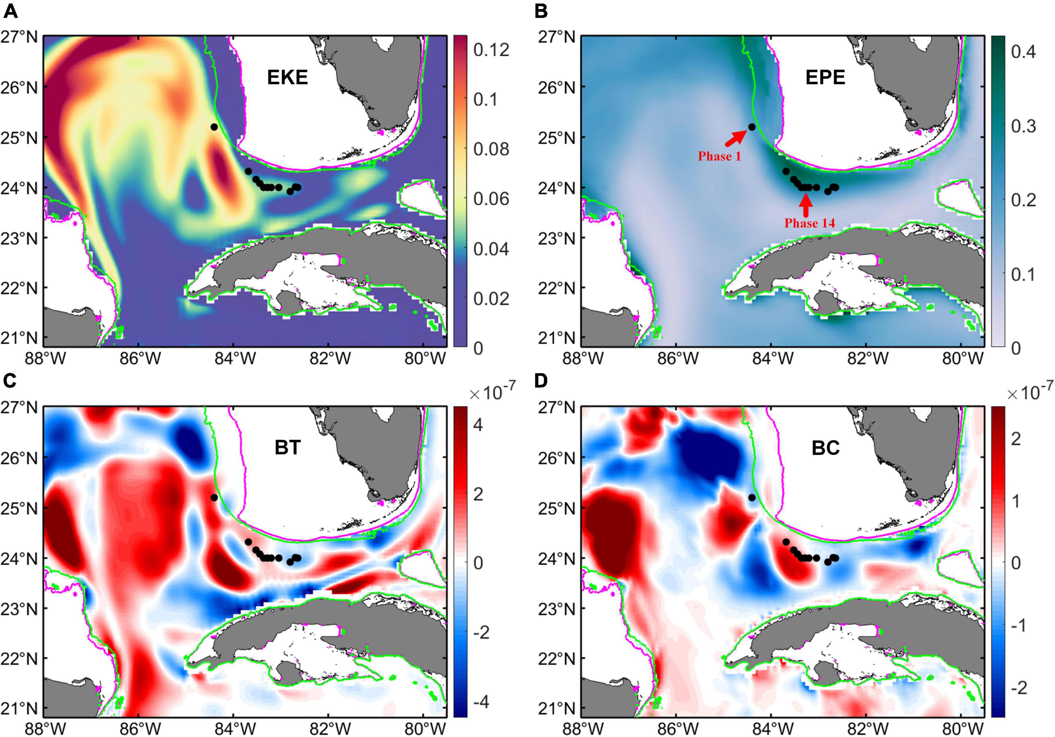
Figure 10. Horizontal distributions of mean (A) EKE (unit: m²/s²), (B) EPE (unit: m²/s²), (C) BT (unit: m²/s³), and (D) BC (unit: m²/s³) from April 9th to August 12th, 2017. These variables are vertically averaged from 0 to 800 m. The black dots on each map denote the eddy centers determined from weekly mean global HYCOM surface current fields during phases 1–14 (Figure 5, April 9 to July 15, 2017), and they are the same as those shown in Figure 6B. The eddy centers during phases 1 and 14 are annotated with red arrows in (B). Calculations are shown for depths greater than 100 m; the 100 and 200 m isobaths are marked with magenta and green lines, respectively.

To further diagnose the energy transfer between the TE and the LC/FC system, we defined the effective eddy region as a circular area which is centered on a model-based eddy center, and has a same radius as the average radius (51.6 km) of the simulated TE during phases 1–14 (April 9 to July 15, 2017). The vertical distributions of EKE, EPE, BT, and BC averaged horizontally over the effective eddy regions during phases 1–14 (April 9 to July 15, 2017) are illustrated in Figure 11. As shown in Figure 11A, larger EKE is found in the upper layer within 300 m depth, and the EKE decreases with water depth, while the EPE shown in Figure 11B reaches its maximum in the middle layer (∼100–500 m). Both EKE and EPE fluctuate with time. Larger EKE is found during the first 6 phases (April 9 to May 20, 2017) while moderate EKE is found during phases 10–14 (June 11 to July 15, 2017), and EKE minimum is found during phases 7–9 (May 21 to June 10, 2017). Note that the EKE during the phase 1 (April 9 to April 15, 2017) is not a small value, this is because the simulated TE was first detected on April 5th instead of April 9th when the observed TE was first detected on altimetry imagery. As shown in Figure 11B, the depth characterized with high EPE was getting deeper during phases 1–11 (April 9 to June 24, 2017), and then getting shallower during phases 12–14 (June 25 to July 15, 2017).

FIGURE 11

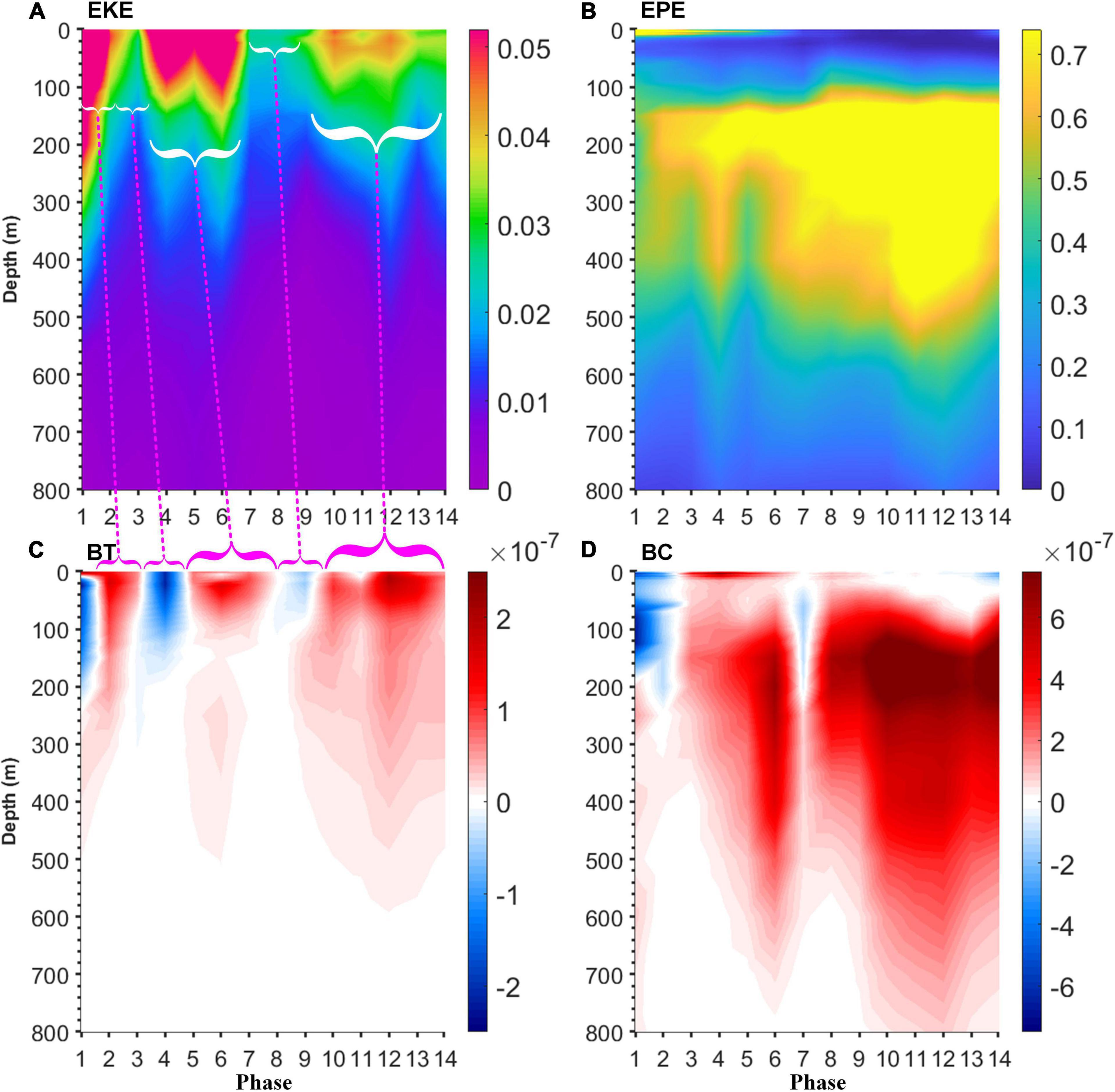
Figure 11. Vertical distributions of (A) EKE (unit: m²/s²), (B) EPE (unit: m²/s²), (C) BT (unit: m²/s³), and (D) BC (unit: m²/s³) averaged horizontally over the effective eddy regions during phases 1–14 (April 9 to July 15, 2017). There is a correspondence between (A,C), as illustrated by the dashed magenta lines.

Large positive BT and BC are found in Figures 11C,D, respectively, during most of phases 1–14 (April 9 to July 15, 2017), this indicates that strong barotropic and baroclinic instability occurred during the evolution of the TE. When linking the vertical distribution of EKE to that of BT, we found an evident time lag between them (BT leads EKE for around 1 phase (week); note the dashed magenta lines between Figures 11A,C). The time lag between EKE and BT is also reported in Cheng et al. (2013), Chen et al. (2016), and Yang et al. (2017). To explore the correlation between BT and EKE, we averaged the EKE and BT for the layer between 0 and 300 m, where both EKE and BT are characterized with large values. After plotting the time series of EKE and BT during phases 1–14 (results not shown here, April 9 to July 15, 2017), there is an apparent 1-week time lag between them before phase 9, and no time lag between them is found after phase 9 (June 4 to June 10, 2017). When considering the time lag of 1 week, the correlation coefficient between the time series of EKE during phases 1–13 (April 9 to July 8, 2017) and the time series of BT during phases 2–14 (April 16 to July 15, 2017) is 0.44 (p-value: 0.13), while the time series of EKE during phases 1–8 (April 9 to June 3, 2017) is significantly correlated (R = 0.74, p-value < 0.05) with that of BT during phases 2–9 (April 16 to June 10, 2017). The correlation coefficient between the time series of EKE and BT during phases 9–14 (June 4 to July 15, 2017) is 0.62 (p-value: 0.19). Similarly, to diagnose the relationship between EPE and BC, we averaged them for the layer of 100–500 m, where they both are characterized with large values. After plotting their time series during phases 1–14 (results not shown here, April 9 to July 15, 2017), no evident time lag is found, and they both are significantly correlated (R = 0.77, p-value < 0.01). High correlations between EKE and BT, and between EPE and BC suggest that barotropic and baroclinic instability have played an important role in the evolution of the TE, and significantly contributed to the modulation of eddy energy during phases 1–14 (April 9 to July 15, 2017).

Positive wind stress curl is favorable for the formation and evolution of CEs (Hwang and Chen, 2000; Nan et al., 2011; Mandal et al., 2019). To assess the effect of wind stress curl on the formation and transition of the TE, we calculated the mean wind stress curl from April 9 to August 12, 2017 (phases 1–18), and plotted the time series of the wind stress curl averaged horizontally over the effective eddy regions during phases 1–14 (April 9 to July 15, 2017). Figure 12 shows the results. Obviously, the model-based eddy centers during phases 1–14 (April 9 to July 15, 2017) shown as green dots in Figure 12A are all located in the region characterized by negative wind stress curl. What’s more, the wind stress curl averaged over the effective eddy regions during phases 1–14 (April 9 to July 15, 2017) are almost all negative as shown in Figure 12B. These results indicate that the wind stress curl was not a favorable condition for the formation and development of the TE.

FIGURE 12

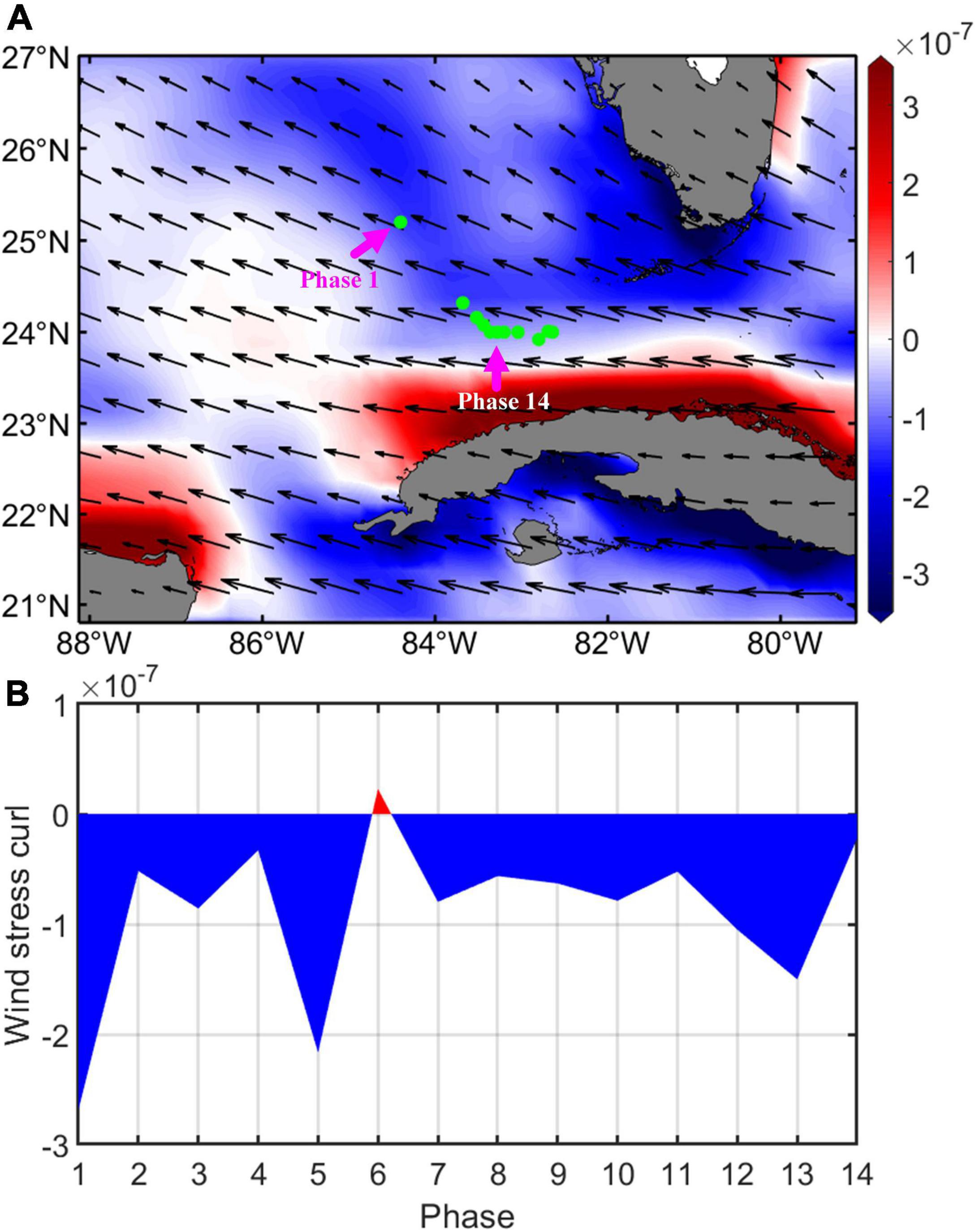
Figure 12. (A) Distribution of mean wind stress curl (color shadings, unit: N/m³) overlaid with the direction of mean wind stress (black vectors) during phases 1–18 (April 9 to August 12, 2017). Green dots represent the eddy centers determined from weekly global HYCOM surface current fields during phases 1–14 (Figure 5, April 9 to July 15, 2017), and they are the same as those shown in Figures 6B,10. The eddy centers during phases 1 and 14 are annotated with magenta arrows. (B) Time series of the wind stress curl averaged horizontally over the effective eddy regions during phases 1–14 (April 9 to July 15, 2017). Blue color and red color denote negative and positive wind stress curl, respectively.

Discussion

The Power of Integration of Observation and Modeling

In this work, a variety of observational data are used together with global HYCOM simulations to study a LC frontal eddy that evolved into a long-lasting TE. Both data sets have their own strengths and limitations. The satellite ocean color measurements showed the strengths of observing color patterns in coastal regions off the DT in all seasons under cloud-free conditions (Zhang et al., 2019). In contrast, SST is nearly isothermal during summer, making it difficult to use to detect and track eddies (e.g., Liu et al., 2011a). Likewise, altimetry-based surface currents may contain large uncertainties in shallow coastal waters. On the other hand, surface drifters, whenever available, are useful to track water masses and to reveal the existence of CEs off the DT (e.g., drifter no. 62283 in Figure 13; also Liu et al., 2011a). In the end, once succesfully evaluated, the global HYCOM provides continuous 3-D data fields that can be used with the AMEDA algorithm to determine the occurrence frequency as well as the 3-D structures of the CEs in the SoF. For example, Figure 14A shows the occurrence frequency of CEs between 2010 and 2015. Following Zu et al. (2013), eddies with a lifespan shorter than 5 days were excluded in our analysis. From Figure 14A, high occurrence of CEs is related to the LC/FC system, and the highest occurrence is found in the eastern branch of the LC and in the coastal area off the DT. Figure 14B further shows the tracks of CEs with a lifespan longer than a month. Some CEs originated from the LC region, which travelled along the LC/FC system and then gradually decayed in the SoF. On the other hand, some CEs formed locally off the DT (e.g., growing from small FC spin-off CEs), and stayed for a long time there until their demise. These results are consistent with the conclusions in Kourafalou and Kang (2012).

FIGURE 13

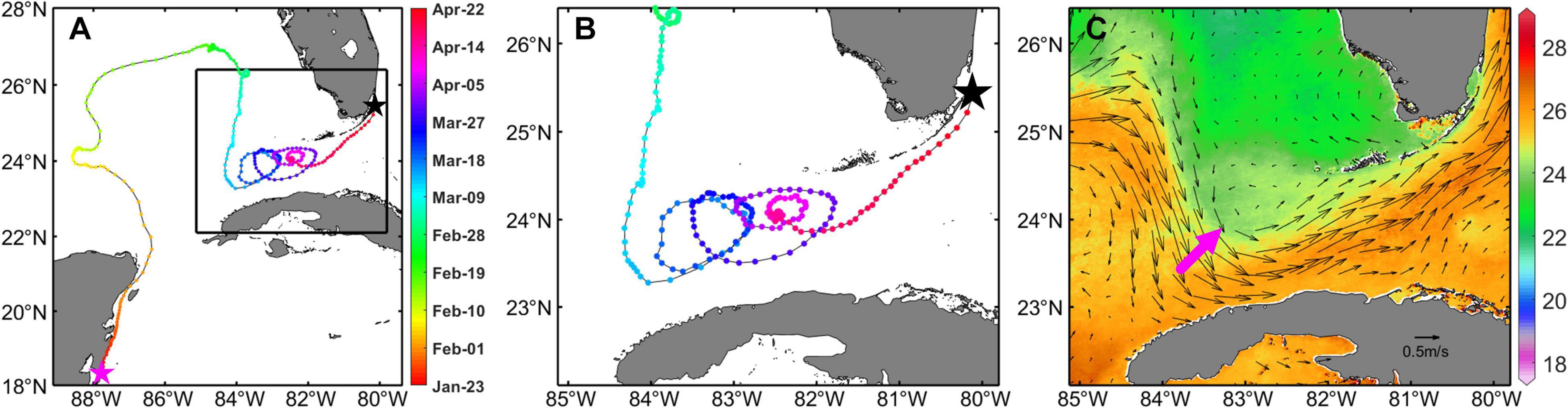
Figure 13. (A) Full trajectory of the drifter no. 62283 from January 23 to April 22, 2007, showing the existence of a CE off the DT. Time is color-coded, and the magenta and black pentagrams represent the start and end points of the drifter, respectively. A region outlined by a black box is enlarged in (B). (C) Distribution of mean MODIS/A SST (color shadings; unit: ^°C) from March 11 to April 18, 2007, during which the drifter was entrained within the CE denoted by a thick magenta arrow. The altimetry-based surface currents averaged over the same period are overlaid as black vectors in (C).

FIGURE 14

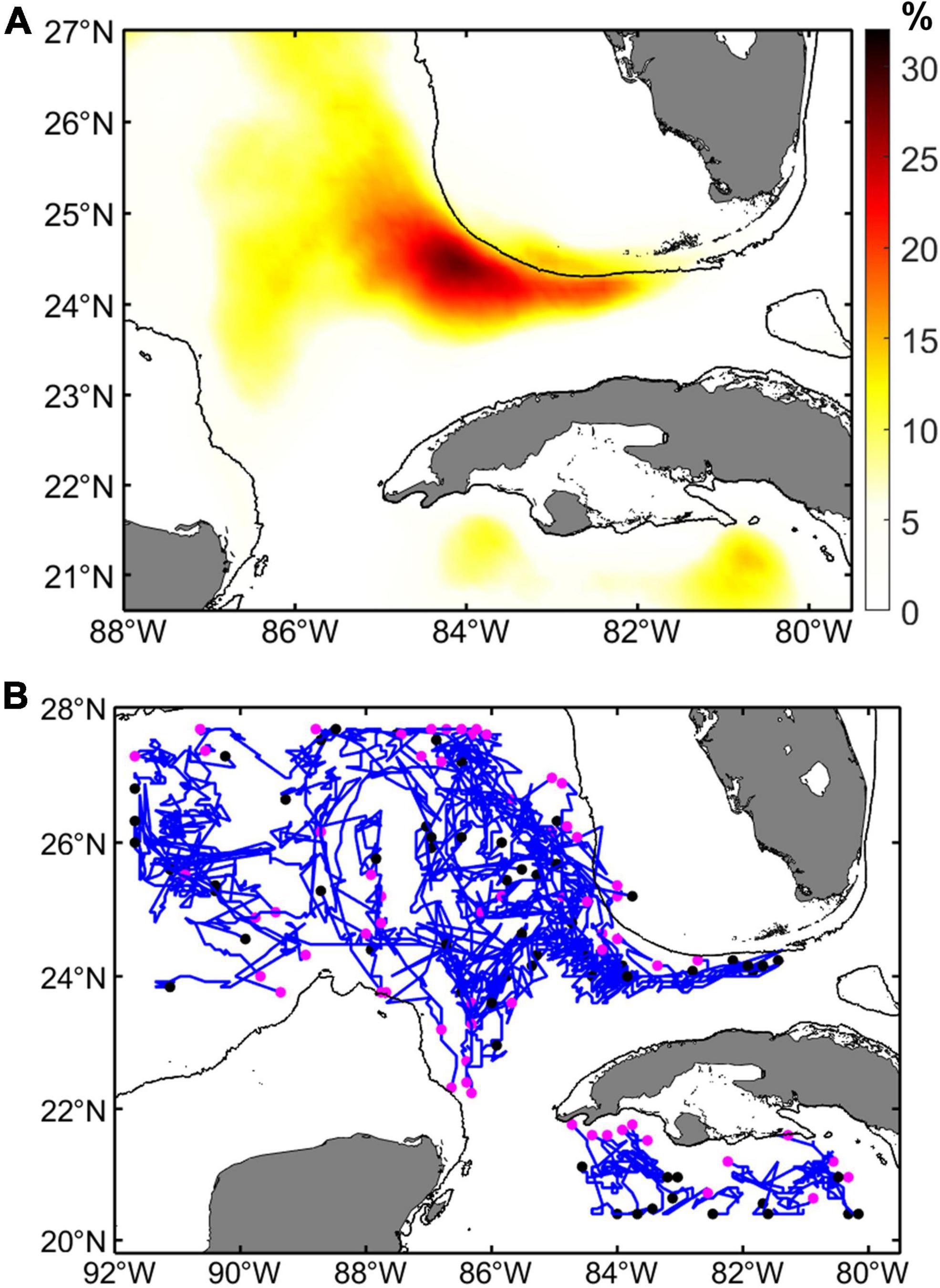
Figure 14. (A) Long-term mean occurrence frequency of the CEs with a lifespan more than 5 days in the southeastern GoM, SoF, and northeastern Caribbean Sea during 2010–2015, derived from global HYCOM simulations. Color shadings represent the percentage of pixels where a location is inside an eddy. (B) Trajectories of CEs with a lifespan longer than 30 days, determined from daily global HYCOM surface current velocity data from 2010 to 2015, based on the AMEDA algorithm. The magenta and black dots in (B), respectively, denote the start and end locations of each eddy track. The 200 m isobath is annotated with black lines in each figure.

Biological and Ecological Implications

The 3-D structure of the TE and its interaction with the LC/FC system have been comprehensively investigated above, based on both model simulations and observational data. The question is: what are their implications on ocean biology and ecology?

Indeed, the long-lasting TE can not only transfer heat, salt, and nutrients, but can also enhance local primary production and entrain biologically rich waters. For example, Kerr et al. (2020) found eggs of reef fish species in deep waters within the TE and eggs of pelagic fish species in shallow nearshore waters off northwestern Cuba; these findings were speculated to be related to the long-lasting TE. Although there is no direct measurement of subsurface Chl or nutrient concentrations within the TE, earlier studies (Hitchcock et al., 2005) on a similar TE indicate that the depth of Chl maximum and nutricline shoaled from around 80 m on the edge of the TE to less than 60 m at the center of the TE, and the highest subsurface Chl concentration (∼1 mg/m³) was observed near the eddy center.

The TE may also have non-local ecological importance. The presence of the TE helps to keep the LC away from direct contact with the “pressure point” of the WFS, which may reduce the offshore forced anomalous upwelling on the shelf and have a consequence for major red tide occurrence on the Florida coast (Liu et al., 2016). The occurrence of TEs may be used to fine tune the seasonal prediction of the red tide on the west Florida coast (Liu et al., 2016; Weisberg et al., 2019).

During the evolution of the TEs and other CEs in the SoF, cyclonic current patterns coupled with prevailing easterly winds can facilitate the onshore advection of larval fish to reef environments located between the DT and the Florida Keys (Lee et al., 1994). Hitchcock et al. (2005) described that nutrients from CEs are very likely to be delivered to the reef environments with the help of physical processes such as breaking internal waves and internal tidal bores when CEs propagate and decay along the Florida Keys (Leichter et al., 1998, 2003). Sponaugle et al. (2005) elaborated on the role of CEs traveling along the FC as means for delivery of coral fish larvae that had been trapped inside the eddy as it passed thorugh the TE spawning grounds; Vaz et al. (2016) showed that such eddies are fundamental in the connectivity of the shallow Florida Keys reefs with upstream mesophotic reef environments (Reed et al., 2018). Some strong and long-lasting CEs can impact the water column extending from surface to more than 700 m, and influence the physical environments and biological productivity throughout the SoF. The frequent occurrence of CEs in the SoF (Figure 14, see also Bulhoes de Morais, 2010; Kourafalou and Kang, 2012; Zhang et al., 2019) makes them particularly relevant to ocean biology and ecology.

Conclusion

Although TEs are well known in the SoF, this is the first time that the entire evolution of a long-lasting TE is studied in detail using multiple means. Specifically, the physical, biochemical, and dynamic characteristics, as well as the 3-D structure of a long-lasting TE are analyzed using several comprehensive datasets. These include observational data from altimeters, ocean color satellites, shipborne ADCP, Argo profiling float, and simulated data from the high-resolution global HYCOM. The long-lasting TE is found to form along the eastern edge of the LC on April 9th, 2017, and remained quasi-stationary for about 3 months off the DT until becoming much smaller due to its interaction with the FC and topography. The TE is characterized with higher Chl and lower temperature than surrounding waters, with a mean diameter of ∼100 km and a penetrating depth of ∼800 m, although its shape is asymmetric. Such long-lasting TEs have been found to have biophysical connectivity implications, e.g., to be responsible for the transport of the eggs of neritic and pelagic fish species within reef environments in the SoF. The study also found consistency between global HYCOM simulations and observational data, and explored the interaction between the LC/FC system and the long-lasting TE from the perspective of energy transfer. Results from the global HYCOM simulations clearly indicate that barotropic and baroclinic instability of the LC/FC system significantly modulated the kinetic and potential energy of the TE, which also played a key role in the growth and evolution of the TE.

Data Availability Statement

All the data used in this study are publicly available Global HYCOM simulations were obtained from https://www.hycom.org/data/glbv0pt08/expt-57pt7 and https://www.hycom.org/data/glbv0pt08/expt-92pt8, as well as from https://www.hycom.org/dataserver/gofs-3pt1/reanalysis. The Argo data were collected and made freely available by the International Argo Program and related national programs (https://argo.ucsd.edu, https://www.oceanops.org). MODIS Aqua Chl imagery were generated and distributed by the Optical Oceanography Laboratory (https://optics.marine.usf.edu) at the University of South Florida. MODIS Aqua and Terra SST imagery were downloaded from the NASA Goddard Space Flight Center (https://oceancolor.gsfc.nasa.gov). The drifter data were provided by the Global Drifter Program at the NOAA/AOML (https://www.aoml.noaa.gov/phod/gdp/). The Version 2 CCMP satellite ocean surface wind vector data were taken from the Remote Sensing Systems website (http://www.remss.com/measurements/ccmp/). The altimetry data products were processed and distributed by the Copernicus Marine Environment Monitoring Service (https://marine.copernicus.eu/).

Author Contributions

YZ: conceptualization, methodology, data processing and analysis, manuscript preparation and revision. CH: conceptualization, methodology, coordination, and manuscript review and revision. VK, YL, DM, and BB: manuscript review and revision. JH: ADCP data processing and manuscript review. All authors contributed to the manuscript and approved the submitted version.

Funding

This work was supported by the NASA student fellowship program “Future Investigators in NASA Earth and Space Science and Technology” (FINESST, 80NSSC19K1358), the National Academies of Sciences, Engineering and Medicine (NASEM) UGOS-1 (2000009918), the NOAA IOOS SECOORA Program [IOOS.21(097)USF.BW.OBS.1], and the NOAA RESTORE Science Program (NA17NOS4510099).

Conflict of Interest

The authors declare that the research was conducted in the absence of any commercial or financial relationships that could be construed as a potential conflict of interest.

Publisher’s Note

All claims expressed in this article are solely those of the authors and do not necessarily represent those of their affiliated organizations, or those of the publisher, the editors and the reviewers. Any product that may be evaluated in this article, or claim that may be made by its manufacturer, is not guaranteed or endorsed by the publisher.

Acknowledgments

We acknowledge the effort from the chief scientist Steve Murawski, the captain and crews onboard the R/V Weatherbird II for collecting the ADCP data. YZ thanks Yingli Zhu and Minghai Huang, as well as Briac Le Vu for helpful discussions on the AMEDA algorithm. We thank the reviewers for their comments and suggestions to help improve the presentation of this manuscript.

Supplementary Material

The Supplementary Material for this article can be found online at: https://www.frontiersin.org/articles/10.3389/fmars.2022.779450/full#supplementary-material

Abbreviations

3-D, 3-dimensional; ADCP, acoustic Doppler current profiler; AMEDA, Angular Momentum Eddy Detection Algorithm; AOML, Atlantic Oceanographic and Meteorological Laboratory; ASCAT, Advanced Scatterometer; AVHRR, Advanced Very High Resolution Radiometer; CCMP, Cross-Calibrated Multi-Platform; CEs, cyclonic eddies; Chl, Chlorophyll; CMEMS, Copernicus Marine Environment Monitoring Service; DAC, Data Assembly Center; DT, Dry Tortugas; EKE, eddy kinetic energy; EPE, eddy potential energy; FC, Florida Current; FINESST, Future Investigators in NASA Earth and Space Science and Technology; GDP, Global Drifter Program; GoM, Gulf of Mexico; HYCOM, Hybrid Coordinate Ocean Model; LC, Loop Current; LC/FC, Loop Current/Florida Current; LNAM, local normalized angular momentum; MLDs, mixed layer depths; MODIS, Moderate Resolution Imaging Spectroradiometer; MODIS/A, Moderate Resolution Imaging Spectroradiometer/Aqua; NASA, National Aeronautics and Space Administration; NOAA, National Oceanic and Atmospheric Administration; NRL-SSC, Naval Research Lab – Stennis Space Center; OW, Okubu-Weiss; QuikSCAT, Quick Scatterometer; RDI, RD Instruments’; RMSD, root-mean-square deviation; ROMS, Regional Ocean Modeling System; RSS, Remote Sensing Systems; R/V, Research Vessel; SCS, South China Sea; SoF, Straits of Florida; SSH, sea surface height; SST, sea surface temperature; TEs, Tortugas eddies; VAM, variational analysis method; WFS, West Florida Shelf; XBTs, expendable bathythermographs; YC, Yucatan Channel.

Footnotes

1. ^ https://argo.ucsd.edu
2. ^ https://www.ocean-ops.org
3. ^ https://www.fio.usf.edu/services/rv-weatherbird/
4. ^ https://www.aoml.noaa.gov/phod/gdp/
5. ^ https://www.aoml.noaa.gov/phod/gdp/interpolated/data/all.php
6. ^ https://oceancolor.gsfc.nasa.gov
7. ^ https://marine.copernicus.eu/
8. ^ http://www.remss.com/measurements/ccmp
9. ^ https://www.hycom.org/
10. ^ https://www.hycom.org/data/glbv0pt08/expt-92pt8
11. ^ https://www.hycom.org/data/glbv0pt08/expt-57pt7
12. ^ https://www.hycom.org/dataserver/gofs-3pt1/reanalysis

References

Argo (2000). Argo float data and metadata from Global Data Assembly Centre (Argo GDAC). SEANOE 2000:42182. doi: 10.17882/42182

PubMed Abstract | CrossRef Full Text | Google Scholar

Brooks, M. T., Coles, V. J., Hood, R. R., and Gower, J. F. (2018). Factors controlling the seasonal distribution of pelagic Sargassum. Mar. Ecol. Prog. Series 599, 1–18. doi: 10.3354/meps12646

CrossRef Full Text | Google Scholar

Bulhoes de Morais, C. R. (2010). On the Evolution of Cyclonic Eddies along the Florida Keys. MS thesis. Coral Gables, Fl: University of Miami, 97.

Google Scholar

Chaigneau, A., Eldin, G., and Dewitte, B. (2009). Eddy activity in the four major upwelling systems from satellite altimetry (1992–2007). Prog. Oceanogr. 83, 117–123. doi: 10.1016/j.pocean.2009.07.012

CrossRef Full Text | Google Scholar

Chaigneau, A., Gizolme, A., and Grados, C. (2008). Mesoscale eddies off Peru in altimeter records: Identification algorithms and eddy spatio-temporal patterns. Prog. Oceanogr. 79, 106–119. doi: 10.1016/j.pocean.2008.10.013

CrossRef Full Text | Google Scholar

Chassignet, E. P., Hurlburt, H. E., Metzger, E. J., Smedstad, O. M., Cummings, J., Halli-well, G. R., et al. (2009). U.S. GODAE: Global ocean prediction with the HYbrid Coordinate Ocean Model (HYCOM). Oceanography 22, 48–59. doi: 10.5670/oceanog.2009.39

CrossRef Full Text | Google Scholar

Chassignet, E. P., Hurlburt, H. E., Smedstad, O. M., Halliwell, G. R., Hogan, P. J., Wallcraft, A. J., et al. (2007). The HYCOM (hybrid coordinate ocean model) data assimilative system. J. Mar. Syst. 65, 60–83. doi: 10.1016/j.marpolbul.2011.06.026

PubMed Abstract | CrossRef Full Text | Google Scholar

Chelton, D. B., Schlax, M. G., and Samelson, R. M. (2011). Global observations of nonlinear mesoscale eddies. Prog. Oceanogr. 91, 167–216.

Google Scholar

Chelton, D. B., Schlax, M. G., Samelson, R. M., and de Szoeke, R. A. (2007). Global observations of large oceanic eddies. Geophys. Res. Lett. 34:L15606. doi: 10.1029/2007GL030812

CrossRef Full Text | Google Scholar

Chen, R., Thompson, A. F., and Flierl, G. R. (2016). Time-dependent eddy-mean energy diagrams and their application to the ocean. J. Phys. Oceanogr. 46, 2827–2850. doi: 10.1175/JPO-D-16-0012.1

CrossRef Full Text | Google Scholar

Chen, S., Hu, C., Barnes, B. B., Xie, Y., Lin, G., and Qiu, Z. (2019). Improving ocean color data coverage through machine learning. Remote Sens. Env. 222, 286–302. doi: 10.1016/j.rse.2018.12.023

CrossRef Full Text | Google Scholar

Cheng, X., Xie, S.-P., McCreary, J. P., Qi, Y., and Du, Y. (2013). Intraseasonal variability of sea surface height in the Bay of Bengal. J. Geophys. Res. Oceans 118:20075. doi: 10.1002/jgrc.20075

CrossRef Full Text | Google Scholar

Chérubin, L. M., Le Paih, N., and Carton, X. (2021). Submesoscale Instability in the Straits of Florida. J. Phys. Oceanogr. 51, 2599–2615. doi: 10.1175/JPO-D-20-0283.1

CrossRef Full Text | Google Scholar

Chew, F. (1974). The turning process in meandering currents: a case study. J. Phys. Oceanogr. 4, 27–57.

Google Scholar

Cleveland, C. A. (2018). Empirical Validation and Comparison of the Hybrid Coordinate Ocean Model (HYCOM) Between the Gulf of Mexico and the Tongue of the Ocean. Master’s thesis. Fort Lauderdale, FL: Nova Southeastern University.

Google Scholar

Criales, M. M., and Lee, T. N. (1996). Larval distribution and transport of penaeoid shrimps during the presence of the Tortugas Gyre in May-June 1991. Oceanogr. Literat. Rev. 6:607.

Google Scholar

Cummings, J. A. (2005). Operational multivariate ocean data assimilation. Q. J. R. Meteorol. Soc. 131, 3583–3604. doi: 10.1256/qj.05.105

CrossRef Full Text | Google Scholar

de Marez, C., Carton, X., L’Hégaret, P., Meunier, T., Stegner, A., Le Vu, B., et al. (2020). Oceanic vortex mergers are not isolated but influenced by the β-effect and surrounding eddies. Sci. Rep. 10, 1–10. doi: 10.1038/s41598-020-59800-y

PubMed Abstract | CrossRef Full Text | Google Scholar

de Marez, C., L’Hégaret, P., Morvan, M., and Carton, X. (2019). On the 3D structure of eddies in the Arabian Sea. Deep Sea Res. Part I 150:103057. doi: 10.1016/j.dsr.2019.06.003

CrossRef Full Text | Google Scholar

Dombrowsky, E., Bertino, L., Brassington, G. B., Chassignet, E. P., Davidson, F., Hurlburt, H. E., et al. (2009). GODAE systems in operation. Oceanography 22, 80–95.

PubMed Abstract | Google Scholar

Dong, C., Lin, X., Liu, Y., Nencioli, F., Chao, Y., Guan, Y., et al. (2012). Three-dimensional oceanic eddy analysis in the Southern California Bight from a numerical product. J. Geophys. Res. 117:C00H14. doi: 10.1029/2011JC007354

CrossRef Full Text | Google Scholar

Donohue, K. A., Watts, D. R., Hamilton, P., Leben, R., and Kennelly, M. (2016). Loop current eddy formation and baroclinic instability. Dyn. Atmosph. Oceans 76, 195–216. doi: 10.1016/j.dynatmoce.2016.01.004

CrossRef Full Text | Google Scholar

DuBois, M. J., Putman, N. F., and Piacenza, S. E. (2020). Hurricane frequency and intensity may decrease dispersal of Kemp’s ridley sea turtle hatchlings in the Gulf of Mexico. Front. Mar. Sci. 7:301. doi: 10.3389/fmars.2020.00301

CrossRef Full Text | Google Scholar

Eden, C., and Böning, C. (2002). Sources of eddy kinetic energy in the Labrador Sea. J. Phys. Oceanogr. 32, 3346–3363. doi: 10.1175/1520-0485(2002)032<3346:SOEKEI>2.0.CO;2

CrossRef Full Text | Google Scholar

Faghmous, J. H., Frenger, I., Yao, Y., Warmka, R., Lindell, A., and Kumar, V. (2015). A daily global mesoscale ocean eddy dataset from satellite altimetry. Sci. Data 2, 1–16. doi: 10.1038/sdata.2015.28

PubMed Abstract | CrossRef Full Text | Google Scholar

Feehan, C. J., Sharp, W. C., Miles, T. N., Brown, M. S., and Adams, D. K. (2019). Larval influx of Diadema antillarum to the Florida Keys linked to passage of a Tortugas Eddy. Coral Reefs 38, 387–393. doi: 10.1007/s00338-019-01786-9

CrossRef Full Text | Google Scholar

Firing, E., and Hummon, J. M. (2010). Shipboard ADCP Measurements. The GO-SHIP Repeat Hydrography Manual: A Collection of Expert Reports and Guidelines. IOCCP Report #14. ICPO Publication Series 134; Version 1.

Google Scholar

Fratantoni, P. S., Lee, T. N., Podesta, G. P., and Muller-Karger, F. (1998). The influence of Loop Current perturbations on the formation and evolution of Tortugas eddies in the southern Straits of Florida. J. Geophys. Res. 103, 24759–24779. doi: 10.1029/98JC02147

CrossRef Full Text | Google Scholar

Furey, H., Bower, A., Perez-Brunius, P., Hamilton, P., and Leben, R. (2018). Deep eddies in the Gulf of Mexico observed with floats. J. Phys. Oceanogr. 48, 2703–2719. doi: 10.1175/JPO-D-17-0245.1

CrossRef Full Text | Google Scholar

Halo, I., Backeberg, B., Penven, P., Ansorge, I., Reason, C., and Ullgren, J. E. (2014). Eddy properties in the Mozambique Channel: a comparison between observations and two numerical ocean circulation models. Deep Sea Res. Part II 100, 38–53. doi: 10.1016/j.dsr2.2013.10.015

CrossRef Full Text | Google Scholar

Hamilton, P., Bower, A., Furey, H., Leben, R., and Pérez-Brunius, P. (2019). The Loop Current: observations of deep eddies and topographic waves. J. Phys. Oceanogr. 49, 1463–1483.

PubMed Abstract | Google Scholar

Hamilton, P., Leben, R., Bower, A., Furey, H., and Pérez-Brunius, P. (2018). Hydrography of the Gulf of Mexico using autonomous floats. J. Phys. Oceanogr. 48, 773–794. doi: 10.1371/journal.pone.0101658

PubMed Abstract | CrossRef Full Text | Google Scholar

Hitchcock, G. L., Lee, T. N., Ortner, P. B., Cummings, S., Kelble, C., and Williams, E. (2005). Property fields in a Tortugas Eddy in the southern straits of Florida. Deep Sea Res. Part I 52, 2195–2213. doi: 10.1016/j.dsr.2005.08.006

CrossRef Full Text | Google Scholar

Hu, C. (2011). An empirical approach to derive MODIS ocean color patterns under severe sun glint. Geophys. Res. Lett. 38:L01603. doi: 10.1029/2010GL045422

CrossRef Full Text | Google Scholar

Hu, C., Murch, B., Barnes, B. B., Wang, M., Maréchal, J. P., Franks, J., et al. (2016). Sargassum watch warns of incoming seaweed. Eos 97, 10–15. doi: 10.1029/2016EO058355

CrossRef Full Text | Google Scholar

Huang, M., Liang, X., Zhu, Y., Liu, Y., and Weisberg, R. H. (2021). Eddies connect the tropical Atlantic Ocean and the Gulf of Mexico. Geophys. Res. Lett. 48:e2020GL091277. doi: 10.1029/2020GL091277

CrossRef Full Text | Google Scholar

Hwang, C., and Chen, S.-A. (2000). Circulations and eddies over the South China Sea derived from TOPEX/Poseidon altimetry. J. Geophys. Res. 105, 23943–23965. doi: 10.1029/2000JC900092

CrossRef Full Text | Google Scholar

Ioannou, A., Stegner, A., Le Vu, B., Taupier-Letage, I., and Speich, S. (2017). Dynamical evolution of intense Ierapetra eddies on a 22 year long period. J. Geophys. Res. 122, 9276–9298. doi: 10.1002/2017JC013158

CrossRef Full Text | Google Scholar

Johns, E. M., Lumpkin, R., Putman, N. F., Smith, R. H., Muller-Karger, F. E., Rueda-Roa, D. T., et al. (2020). The establishment of a pelagic Sargassum population in the tropical Atlantic: Biological consequences of a basin-scale long distance dispersal event. Progress in Oceanography 182:102269. doi: 10.1016/j.pocean.2020.102269

CrossRef Full Text | Google Scholar

Kang, D., and Curchitser, E. N. (2013). Gulf Stream eddy characteristics in a high-resolution ocean model. J. Geophys. Res. 118, 4474–4487. doi: 10.1002/jgrc.20318

CrossRef Full Text | Google Scholar

Kerr, M., Browning, J., Bønnelycke, E. M., Zhang, Y., Hu, C., Armenteros, M., et al. (2020). DNA barcoding of fish eggs collected off northwestern Cuba and across the Florida Straits demonstrates egg transport by Mesoscale eddies. Fish. Oceanogr. 29, 340–348. doi: 10.1111/fog.12475

CrossRef Full Text | Google Scholar

Kourafalou, V. H., Androulidakis, Y. S., Kang, H., Smith, R. H., and Valle-Levinson, A. (2018). Physical connectivity between Pulley Ridge and Dry Tortugas coral reefs under the influence of the Loop Current/Florida Current system. Prog. Oceanogr. 165, 75–99. doi: 10.1016/j.pocean.2018.05.004

CrossRef Full Text | Google Scholar

Kourafalou, V. H., and Kang, H. (2012). Florida Current meandering and evolution of cyclonic eddies along the Florida Keys Reef Tract: Are they interconnected? J. Geophys. Res. 117:C05028. doi: 10.1029/2011JC007383

CrossRef Full Text | Google Scholar

Large, W. G., McWilliams, J. C., and Doney, S. C. (1994). Oceanic vertical mixing: a review and a model with a nonlocal boundary layer parameterization. Rev. Geophys. 32, 363–403. doi: 10.1029/94rg01872

CrossRef Full Text | Google Scholar

Laxenaire, R., Speich, S., and Stegner, A. (2019). Evolution of the thermohaline structure of one Agulhas ring reconstructed from satellite altimetry and Argo floats. J. Geophys. Res. 124, 8969–9003. doi: 10.1029/2019JC015210

CrossRef Full Text | Google Scholar

Le Hénaff, M., and Kourafalou, V. H. (2016). Mississippi waters reaching South Florida reefs under no flood conditions: synthesis of observing and modeling system findings. Ocean Dyn. 66, 435–459. doi: 10.1007/s10236-016-0932-4

CrossRef Full Text | Google Scholar

Le Hénaff, M., Kourafalou, V. H., Androulidakis, Y., Smith, R. H., Kang, H., Hu, C., et al. (2020). In situ measurements of circulation features influencing cross-shelf transport around northwest Cuba. J. Geophys. Res. 125:e2019JC015780. doi: 10.1029/2019JC015780

CrossRef Full Text | Google Scholar

Le Hénaff, M., Kourafalou, V. H., Morel, Y., and Srinivasan, A. (2012). Simulating the dynamics and intensification of cyclonic Loop Current Frontal Eddies in the Gulf of Mexico. J. Geophys. Res. 117:C02034. doi: 10.1029/2011JC007279

CrossRef Full Text | Google Scholar

Le Vu, B., Stegner, A., and Arsouze, T. (2018). Angular Momentum Eddy Detection and tracking Algorithm (AMEDA) and its application to coastal eddy formation. J. Atmosph. Oceanic Tech. 35, 739–762. doi: 10.1175/JTECH-D-17-0010.1

CrossRef Full Text | Google Scholar

Lee, T. N., Clarke, M. E., Williams, E., Szmant, A. F., and Berger, T. (1994). Evolution of the Tortugas Gyre and its influence on recruitment in the Florida Keys. Bull. Mar. Sci. 54, 621–646.

Google Scholar

Lee, T. N., Leaman, K., Williams, E., Berger, T., and Atkinson, L. (1995). Florida Current meanders and gyre formation in the southern Straits of Florida. J. Geophys. Res. 100, 8607–8620. doi: 10.1029/94JC02795

CrossRef Full Text | Google Scholar

Lee, T. N., Rooth, C., Williams, E., McGowan, M., Szmant, A. F., and Clarke, M. E. (1992). Influence of Florida Current, gyres and wind-driven circulation on transport of larvae and recruitment in the Florida Keys coral reefs. Contin. Shelf Res. 12, 971–1002. doi: 10.1016/0278-4343(92)90055-O

CrossRef Full Text | Google Scholar

Leichter, J. J., Shellenbarger, G., Genovese, S. J., and Wing, S. R. (1998). Breaking internal waves on a Florida (USA) coral reef: a plankton pump at work? Mar. Ecol. Prog. Ser. 166, 83–97. doi: 10.3354/meps166083

CrossRef Full Text | Google Scholar

Leichter, J. J., Stewart, H. L., and Miller, S. L. (2003). Episodic nutrient transport to Florida coral reefs. Limnol. Oceanogr. 48, 1394–1407. doi: 10.4319/lo.2003.48.4.1394

CrossRef Full Text | Google Scholar

Li, Y., Li, X., Wang, J., and Peng, S. (2016). Dynamical analysis of a satellite-observed anticyclonic eddy in the northern Bering Sea. J. Geophys. Res. 121, 3517–3531. doi: 10.1002/2015JC011586

CrossRef Full Text | Google Scholar

Limouzy-Paris, C. B., Graber, H. C., Jones, D. L., Röpke, A. W., and Richards, W. J. (1997). Translocation of larval coral reef fishes via sub-mesoscale spin-off eddies from the Florida Current. Bull. Mar. Sci. 60, 966–983.

Google Scholar

Lin, X., Dong, C., Chen, D., Liu, Y., Yang, J., Zou, B., et al. (2015). Three-dimensional properties of mesoscale eddies in the South China Sea based on eddy-resolving model output. Deep Sea Res. Part I 99, 46–64. doi: 10.1016/j.dsr.2015.01.007

CrossRef Full Text | Google Scholar

Liu, Y., Dong, C., Guan, Y., Chen, D., McWilliams, J., and Nencioli, F. (2012). Eddy analysis in the subtropical zonal band of the North Pacific Ocean. Deep Sea Res. Part I 68, 54–67. doi: 10.1016/j.dsr.2012.06.001

CrossRef Full Text | Google Scholar

Liu, Y., Merz, C. R., Weisberg, R. H., Shay, L. K., Glenn, S., and Smith, M. (2021). “An initial evaluation of High-Frequency Radar radial currents in the Straits of Florida in comparison with altimetry and model products,” in Ocean Remote Sensing Technologies: High Frequency, Marine and GNSS-Based Radar, eds W. Huang and E. Gill (Herts: The Institution of Engineering and Technology), 117–144. doi: 10.1049/SBRA537E_ch5

CrossRef Full Text | Google Scholar

Liu, Y., Weisberg, R. H., Hu, C., Kovach, C., and Riethmüller, R. (2011a). “Evolution of the loop current system during the Deepwater Horizon oil spill event as observed with drifters and satellites,” in Monitoring and Modeling the Deepwater Horizon Oil Spill: A Record-Breaking Enterprise. Geophys. Monogr. Ser., Vol. 195, eds Y. Liu, A. MacFadyen, Z.-G. Ji, and R. H. Weisberg (Washington, DC: The American Geophysical Union), 91–101. doi: 10.1029/2011GM001127

CrossRef Full Text | Google Scholar

Liu, Y., Weisberg, R. H., Hu, C., and Zheng, L. (2011b). Tracking the Deepwater Horizon oil spill: a modeling perspective. Eos. Transact. Am. Geophys. Union 92, 45–46. doi: 10.1029/2011EO060001

CrossRef Full Text | Google Scholar

Liu, Y., Weisberg, R. H., Hu, C., and Zheng, L. (2011c). “Trajectory forecast as a rapid response to the Deepwater Horizon oil spill,” in Monitoring and Modeling the Deepwater Horizon Oil Spill: A Record-Breaking Enterprise. Geophys. Monogr. Ser., Vol. 195, eds Y. Liu, A. MacFadyen, Z.-G. Ji, and R. H. Weisberg (Washington, DC: The American Geophysical Union), 153–165. doi: 10.1029/2011GM001121

CrossRef Full Text | Google Scholar

Liu, Y., Weisberg, R. H., Lenes, J. M., Zheng, L., Hubbard, K., and Walsh, J. J. (2016). Offshore forcing on the “pressure point” of the West Florida Shelf: Anomalous upwelling and its influence on harmful algal blooms. J. Geophys. Res. Oceans 121, 5501–5515. doi: 10.1002/2016JC011938

CrossRef Full Text | Google Scholar

Luecke, C. A., Arbic, B. K., Bassette, S. L., Richman, J. G., Shriver, J. F., Alford, M. H., et al. (2017). The global mesoscale eddy available potential energy field in models and observations. J. Geophys. Res. 122, 9126–9143. doi: 10.1002/2017JC013136

CrossRef Full Text | Google Scholar

Luo, J., Ault, J. S., Shay, L. K., Hoolihan, J. P., Prince, E. D., Brown, C. A., et al. (2015). Ocean heat content reveals secrets of fish migrations. PLoS One 10:e0141101. doi: 10.1371/journal.pone.0141101

PubMed Abstract | CrossRef Full Text | Google Scholar

Mandal, S., Sil, S., Pramanik, S., Arunraj, K. S., and Jena, B. K. (2019). Characteristics and evolution of a coastal mesoscale eddy in the Western Bay of Bengal monitored by high-frequency radars. Dyn. Atmosph. Oceans 88: 101107.

Google Scholar

Martínez, S., Carrillo, L., and Marinone, S. G. (2019). Potential connectivity between marine protected areas in the Mesoamerican Reef for two species of virtual fish larvae: Lutjanus analis and Epinephelus striatus. Ecol. Indicat. 102, 10–20. doi: 10.1016/j.ecolind.2019.02.027

CrossRef Full Text | Google Scholar

Martínez, S., Carrillo, L., Sosa-Cordero, E., Vásquez-Yeomans, L., Marinone, S. G., and Gasca, R. (2020). Retention and dispersion of virtual fish larvae in the Mesoamerican Reef. Reg. Stud. Mar. Sci. 37:101350. doi: 10.1016/j.rsma.2020.101350

CrossRef Full Text | Google Scholar

Metzger, E., Helber, R. W., Hogan, P. J., Posey, P. G., Thoppil, P. G., Townsend, T. L., et al. (2017). Global Ocean Forecast System 3.1 validation test. Technical Report. NRL/MR/7320–17-9722. Hancock, MS: Stennis Space Center, 61. doi: 10.21236/AD1034517

CrossRef Full Text | Google Scholar

Metzger, E. J., Smedstad, O. M., Thoppil, P., Hurlburt, H. E., Wallcraft, A. J., Franklin, D. S., et al. (2008). Validation Test Report for the Global Ocean Predictions System V3.0 - 1/12^° HYCOM/NCODA: Phase I. NRL Memorandum Report, NRL/MR/7320–08-9148.

Google Scholar

Metzger, E. J., Smedstad, O. M., Thoppil, P. G., Hurlburt, H. E., Cummings, J. A., Wallcraft, A. J., et al. (2014). US Navy Operational Global ocean and Arctic ice prediction systems. Oceanography 27, 32–43.

Google Scholar

Mezić, I., Loire, S., Fonoberov, V. A., and Hogan, P. (2010). A new mixing diagnostic and Gulf oil spill movement. Science 330, 486–489. doi: 10.1126/science.1194607

PubMed Abstract | CrossRef Full Text | Google Scholar

Morvan, M., L’Hégaret, P., de Marez, C., Carton, X., Corréard, S., and Baraille, R. (2020). Life cycle of mesoscale eddies in the Gulf of Aden. Geophys. Astrophys. Fluid Dyn. 114, 631–649.

Google Scholar

Nan, F., Xue, H., Xiu, P., Chai, F., Shi, M., and Guo, P. (2011). Oceanic eddy formation and propagation southwest of Taiwan. J. Geophys. Res. 116:C12045. doi: 10.1029/2011JC007386

CrossRef Full Text | Google Scholar

Nencioli, F., Dong, C., Dickey, T., Washburn, L., and McWilliams, J. C. (2010). A vector geometry–based eddy detection algorithm and its application to a high-resolution numerical model product and high-frequency radar surface velocities in the Southern California Bight. J. Atmosph. Oceanic Technol. 27, 564–579. doi: 10.1175/2009jtecho725.1

CrossRef Full Text | Google Scholar

Oey, L. Y. (2008). Loop Current and deep eddies. J. Phys. Oceanogr. 38, 1426–1449. doi: 10.1175/2007jpo3818.1

CrossRef Full Text | Google Scholar

Oke, P. R., and Griffin, D. A. (2011). The cold-core eddy and strong upwelling off the coast of New South Wales in early 2007. Deep Sea Res. II Top. Stud. Oceanogr. 58, 574–591.

Google Scholar

Okubo, A. (1970). Horizontal dispersion of floatable particles in the vicinity of velocity singularities such as convergences in Deep sea research and oceanographic abstracts, Vol. 17. Amsterdam: Elsevier, 445–454. doi: 10.1016/0011-7471(70)90059-8

CrossRef Full Text | Google Scholar

Paris, C. B., Vaz, A. C., Berenshtein, I., Perlin, N., Faillettaz, R., Aman, Z. M., et al. (2020). Simulating deep oil spills beyond the Gulf of Mexico in Scenarios and Responses to Future Deep Oil Spills. Cham: Springer, 315–336. doi: 10.1007/978-3-030-12963-7_19

CrossRef Full Text | Google Scholar

Parks, A. B., Shay, L. K., Johns, W. E., Martinez-Pedraja, J., and Gurgel, K.-W. (2009). HF radar observations of small-scale surface current variability in the Straits of Florida. J. Geophys. Res. 114:C08002. doi: 10.1029/2008JC005025

CrossRef Full Text | Google Scholar

Pegliasco, C., Chaigneau, A., Morrow, R., and Dumas, F. (2021). Detection and tracking of mesoscale eddies in the Mediterranean Sea: a comparison between the Sea Level Anomaly and the Absolute Dynamic Topography fields. Adv. Space Res. 68, 401–419. doi: 10.1016/j.asr.2020.03.039

CrossRef Full Text | Google Scholar

Porch, C. E. (1998). A numerical study of larval fish retention along the southeast Florida coast. Ecol. Model. 109, 35–59. doi: 10.1016/S0304-3800(98)00005-2

CrossRef Full Text | Google Scholar

Putman, N. F., Goni, G. J., Gramer, L. J., Hu, C., Johns, E. M., Trinanes, J., et al. (2018). Simulating transport pathways of pelagic Sargassum from the Equatorial Atlantic into the Caribbean Sea. Prog. Oceanogr. 165, 205–214. doi: 10.1016/j.pocean.2018.06.009

CrossRef Full Text | Google Scholar

Putman, N. F., and He, R. (2013). Tracking the long-distance dispersal of marine organisms: sensitivity to ocean model resolution. J. R. Soc. Interf. 10:20120979. doi: 10.1098/rsif.2012.0979

PubMed Abstract | CrossRef Full Text | Google Scholar

Putman, N. F., Seney, E. E., Verley, P., Shaver, D. J., López-Castro, M. C., Cook, M., et al. (2020a). Predicted distributions and abundances of the sea turtle ‘lost years’ in the western North Atlantic Ocean. Ecography 43, 506–517. doi: 10.1111/ecog.04929

CrossRef Full Text | Google Scholar

Putman, N. F., Lumpkin, R., Olascoaga, M. J., Trinanes, J., and Goni, G. J. (2020b). Improving transport predictions of pelagic Sargassum. J. Exp. Mar. Biol. Ecol. 529:151398. doi: 10.1016/j.jembe.2020.151398

CrossRef Full Text | Google Scholar

Qian, S., Wei, H., Xiao, J. G., and Nie, H. (2018). Impacts of the Kuroshio intrusion on the two eddies in the northern South China Sea in late spring 2016. Ocean Dyn. 68, 1695–1709. doi: 10.1007/s10236-018-1224-y

CrossRef Full Text | Google Scholar

Reed, J. K., Farrington, S., David, A., Harter, S., Pomponi, S., Diaz, C., et al. (2018). “Pulley Ridge, Gulf of Mexico, U.S.A,” in Mesophotic Reefs of the World, eds K. Puglise and Y. Loya (New York, NY: Springer publisher), doi: 10.1007/978-3-319-92735-0_4

CrossRef Full Text | Google Scholar

Richardson, D. E., Llopiz, J. K., Leaman, K. D., Vertes, P. S., Muller-Karger, F. E., and Cowen, R. K. (2009). Sailfish (Istiophorus platypterus) spawning and larval environment in a Florida Current frontal eddy. Prog. Oceanogr. 82, 252–264. doi: 10.1016/j.pocean.2009.07.003

CrossRef Full Text | Google Scholar

Sadarjoen, I. A., and Post, F. H. (2000). Detection, quantification, and tracking of vortices using streamline geometry. Comp. Graph. 24, 333–341. doi: 10.1016/S0097-8493(00)00029-7

CrossRef Full Text | Google Scholar

Schiller, A., and Oke, P. R. (2015). Dynamics of ocean surface mixed layer variability in the Indian Ocean. J. Geophys. Res. Oceans 120, 4162–4186. doi: 10.1002/2014JC010538

CrossRef Full Text | Google Scholar

Shadle, S., Lestrade, O., Elmer, F., and Hernandez, F. Jr. (2019). Estimation and Comparison of Epiphyte Loading on Holopelagic Sargassum fluitans Collected in the North Atlantic Ocean and the Gulf of Mexico. Gulf Carib. Res. 30, SC42–SC46. doi: 10.18785/gcr.3001.16

CrossRef Full Text | Google Scholar

Shay, L. K., Cook, T. M., Haus, B. K., Martinez, J., Peters, H., Mariano, A. J., et al. (2000). VHF radar detects oceanic submesoscale vortex along Florida coast, Eos Trans. AGU 81, 209–213. doi: 10.1029/00EO00143

CrossRef Full Text | Google Scholar

Shay, L. K., Lee, T. N., Williams, E. J., Graber, H. C., and Rooth, C. G. H. (1998). Effects of low-frequency current variability on near-inertial submesoscale vortices. J. Geophys. Res. 103, 18691–18714. doi: 10.1029/98JC01007

CrossRef Full Text | Google Scholar

Shulzitski, K., Sponaugle, S., Hauff, M., Walter, K., D’Alessandro, E. K., and Cowen, R. K. (2015). Close encounters with eddies: oceanographic features increase growth of larval reef fishes during their journey to the reef. Biol. Lett. 11:20140746. doi: 10.1098/rsbl.2014.0746

PubMed Abstract | CrossRef Full Text | Google Scholar

Shulzitski, K., Sponaugle, S., Hauff, M., Walter, K. D., and Cowen, R. K. (2016). Encounter with mesoscale eddies enhances survival to settlement in larval coral reef fishes. Proc. Natl. Acad. Sci. 113, 6928–6933. pnas.1601606113

Google Scholar

Shulzitski, K., Sponaugle, S., Hauff, M., Walter, K. D., D’Alessandro, E. K., and Cowen, R. K. (2017). Patterns in larval reef fish distributions and assemblages, with implications for local retention in mesoscale eddies. Can. J. Fish. Aquat. Sci. 75, 180–192. doi: 10.1139/cjfas-2016-0304

CrossRef Full Text | Google Scholar

Sponaugle, S., Lee, T., Kourafalou, V., and Pinkard, D. (2005). Florida Current frontal eddies and the settlement of coral reef fishes. Limnol. Oceanogr. 50, 1033–1048. doi: 10.4319/lo.2005.50.4.1033

CrossRef Full Text | Google Scholar

Stegner, A., Le Vu, B., Dumas, F., Ghannami, M. A., Nicolle, A., et al. (2021). Cyclone-Anticyclone asymmetry of eddy detection on gridded altimetry product in the Mediterranean Sea. J. Geophys. Res. 126:e2021JC017475.

Google Scholar

Suca, J. J., Rasmuson, L. K., Malca, E., Gerard, T., and Lamkin, J. T. (2018). Characterizing larval swordfish habitat in the western tropical North Atlantic. Fish. Oceanogr. 27, 246–258. doi: 10.1111/fog.12249

CrossRef Full Text | Google Scholar

Sun, S., Lu, Y., Liu, Y., Wang, M., and Hu, C. (2018). Tracking an oil tanker collision and spilled oils in the East China Sea using multisensor day and night satellite imagery. Geophys. Res. Lett. 45, 3212–3220. doi: 10.1002/2018GL077433

CrossRef Full Text | Google Scholar

Sun, W., Dong, C., Tan, W., and He, Y. (2019). Statistical characteristics of cyclonic warm-core eddies and anticyclonic cold-core eddies in the North Pacific based on remote sensing data. Remote Sens. 11:208. doi: 10.3390/rs11020208

CrossRef Full Text | Google Scholar

Tedesco, P., Gula, J., Ménesguen, C., Penven, P., and Krug, M. J. (2019). Generation of submesoscale frontal eddies in the Agulhas Current. J. Geophys. Res. 124, 7606–7625. doi: 10.1029/2019JC015229

CrossRef Full Text | Google Scholar

Vaz, A. C., Paris, C. B., Olascoaga, M. J., Kourafalou, V. H., Kang, H., and Reed, J. K. (2016). The perfect storm: match-mismatch of bio-physical events drives larval reef fish connectivity between Pulley Ridge mesophotic reef and the Florida Keys. Contin. Shelf Res. 125, 136–146. doi: 10.1016/j.csr.2016.06.012

CrossRef Full Text | Google Scholar

Vukovich, F. M. (1988). On the formation of elongated cold perturbations off the Dry Tortugas. J. Phys. Oceanogr. 18, 1051–1059. doi: 10.1175/1520-0485(1988)018<1051:OTFOEC>2.0.CO;2

CrossRef Full Text | Google Scholar

Wang, G., Chen, D., and Su, J. (2008). Winter eddy genesis in the eastern South China Sea due to orographic wind jets. J. Phys. Oceanogr. 38, 726–732. doi: 10.1175/2007JPO3868.1

CrossRef Full Text | Google Scholar

Weisberg, R. H., and Liu, Y. (2017). On the Loop Current penetration into the Gulf of Mexico. J. Geophys. Res. Oceans 122, 9679–9694. doi: 10.1002/2017JC013330

CrossRef Full Text | Google Scholar

Weisberg, R. H., Liu, Y., Lembke, C., Hu, C., Hubbard, K., and Garrett, M. (2019). The coastal ocean circulation influence on the 2018 West Florida Shelf K. brevis red tide bloom. J. Geophys. Res. Oceans 124, 2501–2512. doi: 10.1029/2018JC014887

CrossRef Full Text | Google Scholar

Weisberg, R. H., Zheng, L., and Liu, Y. (2011). “Tracking subsurface oil in the aftermath of the Deepwater Horizon well blowout,” in Monitoring and Modeling the Deepwater Horizon Oil Spill: A Record-Breaking Enterprise. Geophys. Monogr. Ser., Vol. 195, eds Y. Liu, A. MacFadyen, Z.-G. Ji, and R. H. Weisberg (Washington, DC: The American Geophysical Union), 205–215. doi: 10.1029/2011GM001131

CrossRef Full Text | Google Scholar

Weisberg, R. H., Zheng, L., and Liu, Y. (2017). On the movement of Deepwater Horizon Oil to northern Gulf beaches. Ocean Model. 111, 81–97. doi: 10.1016/j.ocemod.2017.02.002

CrossRef Full Text | Google Scholar

Weiss, J. (1991). The dynamics of enstrophy transfer in two-dimensional hydrodynamics. Physica D 48, 273–294. doi: 10.1016/0167-2789(91)90088-q

CrossRef Full Text | Google Scholar

Wu, R., and Li, C. (2018). Upper ocean response to the passage of two sequential typhoons. Deep Sea Res. Part I 132, 68–79. doi: 10.1016/j.dsr.2017.12.006

CrossRef Full Text | Google Scholar

Yang, Y., Liang, X. S., Qiu, B., and Chen, S. (2017). On the decadal variability of the eddy kinetic energy in the Kuroshio Extension. J. Phys. Oceanogr. 47, 1169–1187. doi: 10.1175/jpo-d-16-0201.1

CrossRef Full Text | Google Scholar

Yang, Y., Weisberg, R. H., Liu, Y., and Liang, X. S. (2020). Instabilities and Multiscale Interactions Underlying the Loop Current Eddy Shedding in the Gulf of Mexico. J. Phys. Oceanogr. 50, 1289–1317. doi: 10.1175/jpo-d-19-0202.1

CrossRef Full Text | Google Scholar

Yeung, C., and Lee, T. N. (2002). Larval transport and retention of the spiny lobster, Panulirus argus, in the coastal zone of the Florida Keys, USA. Fish. Oceanogr. 11, 286–309. doi: 10.1046/j.1365-2419.2002.00209.x

CrossRef Full Text | Google Scholar

Zang, Z., Xue, Z. G., Xu, K., Bentley, S. J., Chen, Q., D’Sa, E. J., et al. (2019). A two decadal (1993–2012) numerical assessment of sediment dynamics in the northern Gulf of Mexico. Water 11:938. doi: 10.3390/w11050938

CrossRef Full Text | Google Scholar

Zhan, P., Subramanian, A. C., Yao, F., Kartadikaria, A. R., Guo, D., and Hoteit, I. (2016). The eddy kinetic energy budget in the Red Sea. J. Geophys. Res. 121, 4732–4747. doi: 10.1002/2015JC011589

CrossRef Full Text | Google Scholar

Zhang, Y., and Hu, C. (2021). Ocean temperature and color frontal zones in the Gulf of Mexico: Where, when, and why. J. Geophys. Res. 126:e2021JC017544. doi: 10.1029/2021JC017544

CrossRef Full Text | Google Scholar

Zhang, Y., Hu, C., Liu, Y., Weisberg, R. H., and Kourafalou, V. H. (2019). Submesoscale and mesoscale eddies in the Florida straits: observations from satellite ocean color measurements. Geophys. Res. Lett. 46, 13262–13270. doi: 10.1029/2019GL083999

CrossRef Full Text | Google Scholar

Zhao, J., Bower, A., Yang, J., Lin, X., and Zhou, C. (2018). Structure and formation of anticyclonic eddies in the Iceland Basin. J. Geophys. Res. 123, 5341–5359. doi: 10.1029/2018JC013886

CrossRef Full Text | Google Scholar

Zhu, Y., and Liang, X. (2020). Coupling of the surface and near-bottom currents in the Gulf of Mexico. J. Geophys. Res. 125:e2020JC016488. doi: 10.1029/2020JC016488

PubMed Abstract | CrossRef Full Text | Google Scholar

Zu, T., Wang, D., Yan, C., Belkin, I., Zhuang, W., and Chen, J. (2013). Evolution of an anticyclonic eddy southwest of Taiwan. Ocean Dyn. 63, 519–531. doi: 10.1007/s10236-013-0612-6

CrossRef Full Text | Google Scholar