 Mia Schumacher1*
 Veerle A. I. Huvenne2
 Colin W. Devey1,3
 Pedro Martínez Arbizu4
 Arne Biastoch1,3
 Stefan Meinecke5
- 1GEOMAR Helmholtz Centre for Ocean Research Kiel, Kiel, Germany
- 2National Oceanography Centre, Southampton, United Kingdom
- 3Kiel University, Kiel, Germany
- 4Senckenberg am Meer, German Center for Marine Biodiversity Research (DZMB), Wilhelmshaven, Germany
- 5Research Vessel, Sonne, Briese Research, Briese Schiffahrts GmbH & Co KG, Leer, Germany
Landscape maps based on multivariate cluster analyses provide an objective and comprehensive view on the (marine) environment. They can hence support decision making regarding sustainable ocean resource handling and protection schemes. Across a large number of scales, input parameters and classification methods, numerous studies categorize the ocean into seascapes, hydro-morphological provinces or clusters. Many of them are regional, however, while only a few are on a basin scale. This study presents an automated cluster analysis of the entire Atlantic seafloor environment, based on eight global datasets and their derivatives: Bathymetry, slope, terrain ruggedness index, topographic position index, sediment thickness, POC flux, salinity, dissolved oxygen, temperature, current velocity, and phytoplankton abundance in surface waters along with seasonal variabilities. As a result, we obtained nine seabed areas (SBAs) that portray the Atlantic seafloor. Some SBAs have a clear geological and geomorphological nature, while others are defined by a mixture of terrain and water body characteristics. The majority of the SBAs, especially those covering the deep ocean areas, are coherent and show little seasonal and hydrographic variation, whereas other, nearshore SBAs, are smaller sized and dominated by high seasonal changes. To demonstrate the potential use of the marine landscape map for marine spatial planning purposes, we mapped out local SBA diversity using the patch richness index developed in landscape ecology. It identifies areas of high landscape diversity, and is a practical way of defining potential areas of interest, e.g. for designation as protected areas, or for further research. Clustering probabilities are highest (100%) in the center of SBA patches and decrease towards the edges (< 98%). On the SBA point cloud which was reduced for probabilities <98%, we ran a diversity analysis to identify and highlight regions that have a high number of different SBAs per area, indicating the use of such analyses to automatically find potentially delicate areas. We found that some of the highlights are already within existing EBSAs, but the majority is yet unexplored.
1 Introduction: landscape maps and the need for objectivity
The ocean environment is perceived as vast and seemingly endlessly variable, and so are its inhabitants. It may be argued that breaking it down into a handful of distinct classes does not account for its diversity. However, if we aim to develop sustainable practices, particularly those grounded in ecosystem-based management (typically using area-based management tools, [e.g., IUCN, 2018)], there is a need to condense this variability into spatially explicit delineations of biological and environmental entities. As such, there is a need to classify the marine ecosystem into ‘provinces’, ‘landscapes’, or ‘habitats’ (Roff et al., 2003). Indeed, Kavanaugh et al. (2016) summarize that, ‘landscapes are conceptual models of systems shaped by the local geomorphology, environmental conditions and biological processes.’
Most classifications to date either start from a biological point of view, based on the knowledge of species distributions and leading to the delineation of biomes or biogeographic provinces (e.g., Watling et al., 2013), or from the physiographic point of view, deploying a classification of the physical environment as a proxy for species niches and habitats (e.g., Harris et al., 2014). Unfortunately, due to the remoteness and challenging sampling conditions in the deep and open ocean, our knowledge of species distributions in the marine realm is still very limited, creating considerable uncertainties in biogeographic classifications of the ocean (e.g. Tyler et al., 2016) despite the significant progress achieved by large research programs such as the Census of Marine Life (Snelgrove, 2010). Predictions of the distribution patterns of species and biomass are typically made using physical environmental variables as predicting factors, given the fact that, particularly at broad scales, the physical environment is one of the main drivers for species occurrence and community composition, and is commonly better known or observed than the species themselves (Gille et al., 2004; Wei et al., 2010; Watling et al., 2013; Morato et al., 2021). This means that the large-scale ecosystem classifications of the oceans (i.e. the European Nature Information System (hereafter EUNIS) by Davies et al., 2004, the Global Seascape Map by Harris and Whiteway, 2009, the Global Open Ocean and Deep Seabed (hereafter GOODS) biogeographic classification by the Intergovernmental Oceanographic Commission (hereafter IOC), 2009, the Global Seafloor Features Map (hereafter GSFM) by Harris et al., 2014, and the Environmental Marine Units (hereafter EMU) by Sayre et al., 2017) typically start with broad divisions of the physical environment, based on key parameters that influence species’ physiology, distribution, and behavior (e.g., depth, temperature, oxygen concentration, and food availability). They provide a first-level insight into the spatial structure of ocean ecosystems and serve as a tool to indicate ecosystem connectivity or patchiness, as well as supporting marine protected area networks assessments (e.g. McQuaid et al., 2020, Popova et al., 2019) or other aspects of marine spatial planning and conservation (Combes et al., 2021).
Since there are already multiple large scale (e.g. Vasquez et al., 2015, Verfaille et al., 2009) or even global ocean classifications, an important question could be: ‘why do we need yet another?’. The answer to this is neither exhaustive nor trivial: there is a need for enhanced objectivity when talking about classifications, as well as for the use of updated and recent data.
Classifying the ocean environment using thresholds that are based on human interpretation of what exists on the seafloor bears the risk of overlooking specific types of marine landscapes by considering only a few aspects of the environment each time and may introduce artificial divisions because of the way people historically looked at ocean maps and biological data (Howell, 2010). In reality, the physical environment is a multivariate continuum. Ideally, all aspects of its character should, a priori, be considered simultaneously and equally weighted when delineating significantly different environmental entities or landscapes. Multivariate data analysis techniques are capable of this, and can take marine landscape classification beyond the initial, manual approach (Kavanaugh et al., 2016). To our knowledge, only two studies exist that have applied this to the global marine environment: the Global Seascapes by Harris & Whiteway (2009) and the Environmental Marine Units (EMU) by Sayre et al. (2017), which aim to take an objective approach using unsupervised classification techniques on datasets that include hydrographic, morphological, and biological variables on a global scale. Harris and Whiteway (2009, their Figure 10) applied an unsupervised isoclass technique, which is comparable to a stepwise (cascaded) K-Means, on six biophysical variables (i.e., depth, seabed slope, sediment thickness, primary production, bottom water dissolved oxygen, and bottom temperature). Sayre et al. (2017) chose the k-means clustering algorithm in their work. Within this study, we aim to expand the range of input variables, including the latest data from recent and fine-scale ocean models. Using density estimation and model-based clustering, we try to overcome shortcomings of the widely used K-Means, or of similar algorithms (e.g. isoclass), such as their sensitivity to the initial cluster centre placement, fixed number of clusters, limitation to spherically shaped clusters, etc. (Press et al., 2007; Sayre et al., 2017).
1.1 Making use of marine landscape maps
As pressures on the ocean floor from e.g., climate change, overfishing and mining increase, it is becoming increasingly urgent to protect key regions by declaring them marine protected areas (MPA). Less than 10% of the ocean realm is under any form of protection today (IUCN, 2021) although there is agreement that protecting 30% of global land and ocean would be beneficial not only for ecosystem and biodiversity recovery but also for the financial and non-monetary economic sector. This has been widely examined in the 30x30 study by Waldron et al. (2020). And although in 2010, the World Park Congress recommended a protection of 30% by 2014, it is widely known that even today this is by far not the case (e.g. O'Leary et al., 2016; IUCN, 2021).
Out of the existing MPAs, only 31% (less than 2% of the entire ocean) enjoy full protection. The remaining 69% are still open to some extent of fishing activities (Turnbull et al., 2021; IUCN, 2021), although No-Take areas, regions that are fully protected, have shown the greatest effectiveness in preserving marine biodiversity and also a capability of re-establishing the complexity of marine ecosystems (Sala & Giakoumi, 2017). Often, a lack of basic knowledge about the deep-sea ecosystems in a particular region of the deep sea can result in it not being considered for protection. Landscape maps may be an aid with this problem, as they highlight, on an ocean basin scale, both coherent marine areas that may have been unknown so far (e.g. Magali et al., 2021) and also regions of high landscape variability. The latter are particularly relevant, because a major criterion for the designation of MPAs or the definition of EBSAs (Ecologically or Biologically Significant Areas) is the assessment of the local environment’s diversity and variability (IUCN, 2018, CBD, 2009). EBSAs are defined by experts, based on seven parameters (Uniqueness or Rarity, Special importance for life history stages of species, Importance for threatened, endangered or declining species and/or habitats, Vulnerability, Fragility, Sensitivity, or Slow recovery, Biological Productivity, Biological Diversity, Naturalness) (CBD 2019). Often, EBSAs can be found in combination with rough topography, for example along seamount chains (e.g. Walvis ridge) or large fracture zones (e.g La Romanche), but also associated to upwelling and open water regions (Convention on Biological Diversity (CBD), 2009). Translated to the landscape map, these would be regions with a high density of different landscapes. We therefore further demonstrate a prospective use of classifications like this by running a quantitative landscape analysis over the final cluster map. It highlights areas of high cluster diversity density and therewith potential regions of interest for future studies or candidates for marine protected area designation.
2 Methods – processing steps
With this study, we aim to reduce human subjectivity in ecosystem classification as far as possible by avoiding setting thresholds between classes and applying an unsupervised multivariate statistical approach. Unsupervised in this sense means that the clustering procedure is an automatic process that recognizes patterns in an unlabeled dataset. This kind of multivariate statistical clustering scheme treats all input variables equally. We believe that this is a more objective way to describe the ocean environment than weighting individual variables.
2.1 Data selection
Deciding on the right input parameters is as fundamental as it is challenging. In an unsupervised cluster analysis, it is this part which can be influenced by human subjectivity the most, with incorrect choices at this stage potentially rendering biased results (Roff et al., 2003; Harris and Whiteway, 2009). We selected data based on the following: ecological understanding described in literature and existing classifications (e.g., Harris and Whiteway, 2009; IOC, 2009; Howell, 2010; Watling et al., 2013; Harris et al., 2014; Sayre et al., 2017; Morato et al., 2021), spatial coverage, resolution, data access, and data format to have a representative sample of ecological determinants and a good exemplification of the seafloor habitat. In our aim to map hydro-morphological provinces of the Atlantic seafloor, the spatial availability of input data is constrained to the Atlantic geographical boundary and further excluded data from the sea surface and the water column (except for the bottom water). Hence in the deep sea, where data presence is scarce (e.g. Clark et al., 2016) and the major area to be classified is below 1,000m water depth, we relied on models and data compilations that are available in full coverage and not in single scattered sample points. We chose the Copernicus Mercator model (hereafter CMEMS) (EU Copernicus Marine Service, 2021) for hydrographic variables and the Satellite Radar Topography Mission version 2 (hereafter SRTM) 15+V2 data (Tozer et al., 2019a) for geomorphological parameters. Furthermore, also GlobSed (Updated Total Sediment Thickness in the World’s Oceans, Straume et al., 2019) and Particulate Organic Carbon (POC) flux (Lutz, 2007) were chosen as determinant variables. All data were unprojected and were referenced to World Geodetic System (WGS) 84.
2.2 Data acquisition and description
2.2.1 CMEMS data products
Global physical and biochemical data from satellite observations, ocean models, and in-situ samples are combined and published on a regular basis by CMEMS and provide information on the physical and biochemical state, dynamics, and variability of the ocean ecosystem. All data products are freely available to the public (EU Copernicus Marine Service, 2021).
The data used for this study are based on numerical models (NEMO 3.1, ORCA12) and data assimilation techniques (reduced order Kalman filter) (Lellouche et al., 2018). From these, we extracted the following parameters:
* Bottom temperature in [°C] (physical), resolution 1/12°
* Salinity in [psu] (physical), resolution 1/12°
* East (uo) and north (vo) components of ocean currents in [m/s] (physical), resolution 1/12°
* Oxygen in [mmol/m^3] (biochemical), resolution ¼ °
* Phytoplankton in [mol] (biochemical) expressed as carbon in sea water, resolution ¼ °
CMEMS provides all hydrographic data products via FTP server download as global multiband and multi - dimensional NetCDF files. The dimensions are time, latitude, longitude, depth (50 layers), and 11 value variables (salinity, oxygen, etc.).
The physical data product (GLOBAL_ANALYSIS_FORECAST_PHY_001_024_monthly) is based on the PSY4V3 Mercator system of the NEMO 3.1 model and amongst others contains 3D monthly mean fields for temperature, salinity, and current velocity. These data have a horizontal resolution of 1/12° (approximately 8 km at the equator) with 50 depth levels and a vertical resolution of 1m at the sea surface and 450m at the seafloor depth level (Lellouche et al., 2018; Tressol et al., 2020; Chune et al., 2020).
The biochemical data products (GLOBAL_ANALYSIS_FORECAST_BIO_001_028) are based on the PISCES-v2 (Pelagic Interactions Scheme for Carbon and Ecosystem Studies volume 2) model within NEMO 3.6 which simulates biochemical and lower trophic levels of marine ecosystems, as well as carbon and main nutrient cycles (Aumont et al., 2015). It also contains 3D monthly mean fields for oxygen and phytoplankton and comes with a horizontal resolution of ¼° (approximately 24 km at the equator). Similar to the physical data, it has 50 depth levels at a vertical resolution of 1m on the sea surface and 450 m at the seafloor depth level (Paul, 2019).
For our analysis, the selected hydrographic data were reduced to seafloor level (i.e., taking the CMEMS depth layers closest to seafloor), averaged over three years (2018 - 2020) and, additionally, three years’ seasonal variability was calculated. We considered three years a reasonable time scale to capture annual changes and seasonal variability at the same time. An overview of all input variables and their main statistics is listed in the supplementary material. A detailed description of the data preparation and processing is given in sections 2.3 & 2.4.
2.2.2 SRTM15+ V2
The latest Shuttle Radar Topography Mission (SRTM) version 2 digital topographic dataset released by NASA in 2015 is the basis to the topography determinants in our classification. Depending on the satellites’ track spacing, latitude, and water depth, the resolution of the predicted bathymetry is approximately 6 km (Tozer et al., 2019a).
The SRTM15+ V2 grid is available via OpenTopography (https://opentopography.org) as a global NetCDF. It is a data compilation built by Tozer et al. (2019a) of the SRTM predicted ocean depth complemented by shipborne MBES bathymetry at 15” (1/240°) resolution. To avoid bias towards higher resolution data during the classification, the SRTM15+ V2 has been down-sampled to the CMEMS data product resolution of 1/12° (Yesson et al., 2011a, b). The bathymetry grid by Tozer et al. (2019b) was used. Slope, terrain ruggedness (after Riley et al., 1999) and topographic position index (a landform analysis where each data point’s altitude is evaluated to its surrounding neighbors, after Weiss, 2001) were calculated from the depth grid.
2.2.3 Global sediment layer thickness and POC flux
The latest compilation for sediment thickness data GlobSed (Straume et al., 2019) was selected as a further determining variable as sedimentation is a crucial indicator for ecosystem types and biodiversity (e.g., Snelgrove, 1999; Zeppilli et al., 2016). It was also used as a proxy for the sedimentation rate since there is currently no Atlantic-wide full-coverage dataset that reflects sedimentation rate across the basin. GlobSed is the most updated version of global sedimentation information and has been constructed at the same resolution as the CMEMS data (1/12°). Particulate Organic Carbon (POC) flux (Lutz et al., 2007) has further been chosen as a proxy for food availability at the seafloor in addition to phytoplankton (from CMEMS) (e.g. Kharbush et al., 2020). The original grid of resolution of 1/11° was rescaled to 1/12°.
2.3 Data pre-processing
The pre-processing was carried out using gdal (GDAL/OGR 2021), Python V3.7 (Van Rossum & Drake, 2009), and GMT Generic mapping Tools V6.1.1 (Wessel et al., 2019). The results were visualized with QGIS V3.16 (Hannover) (QGIS Development Team, 2020). The following pre-processing steps were made:
1. Apply scale factor and offset to unpack real values from packed netCDF file format (Chune et al., 2020)
2. Create a seafloor layer, if necessary (from those data including the entire water column, e.g. salinity). Resample each input raster at an equal resolution of 1/12° using the grdsample algorithm within GMT.
3. For bathymetry only: calculate derivatives slope, TPI, TRI
4. For partial current velocity components: Calculate absolute velocity using:
v = sqrt(uo2 + vo2)
where vo, uo are north and east current velocity components, respectively
5. For non-static variables: Calculate three-years mean using: [(Jan18 + Jan19 + Jan20) + (Feb18 +)… + (Dec20)]/36
6. For non-static variables: Calculate seasonal variability as:
|summer – winter| where: Summer = (June + July + Aug.)/3 and Winter = (Dec. + Jan. + Feb.)/3
7. ‘Nan out’ landmass: Uniquely fill land areas with NaNs to indicate a lack of relevant oceanic data here and so exclude them from the analysis.
2.4 Data clustering
To find and define clusters, we applied a density estimation and model-based clustering method that is implemented by (finite) Gaussian mixture models (GMM) in R v4.1 (R Core Team 2018). This technique reveals latent structures within the dataset by seeking an optimal number of Gaussian distributions that sufficiently represent the dataset (Hastie et al., 2001). The distributions are fitted iteratively with maximum likelihood implemented by Expectation Maximization (EM) methods. For each point of the dataset, the probability of it belonging to a certain cluster of distributions is estimated (expectation, E-step) using each distribution’s current mean, its covariance matrix, and a hidden mixing probability coefficient as fitting parameters. The expectation step is then repeated (maximization, M-step) until convergence (stabilization of the model) occurs (Hastie et al., 2001; Scrucca and Raftery, 2014). The optimum model (= best number of clusters) is selected by the Bayesian Information Criterion (BIC) index which is known to be robust against overfitting (Press et al., 2007). The E-M-step is somewhat analogous to calculating the distance of each point to the cluster center for a data point in KMeans. In fact, KMeans is a special, simplified case of GMM (Press et al., 2007). GMM however has advantages over KMeans: The number of clusters does not have to be known à priori; GMM takes clusters of various shape, volume, and orientation and is not sensitive to the initial placement of cluster centres, whereas KMeans only accepts spherically shaped clusters. Given that it is based on probability, GMM cluster boundaries are not sharp (i.e. either a point belongs to a cluster or not) but soft, meaning that there is a certain probability that a data point is part of a cluster.
To assess whether to include or exclude variables as input parameters, the variable selection algorithm clustvarsel v2.3.4 (Scrucca & Raftery, 2018) is run before the actual clustering. It examines the differences of BIC indices depending on whether a variable has clustering properties or not. Based on this, a variable is accepted or rejected. A large positive BIC difference indicates high clustering properties (Scrucca and Raftery, 2014). The algorithm accepted all input variables as input parameters, hence this step will not be further discussed. The main steps of the clustering process are listed below.
1. The input parameters were scaled to avoid bias towards extreme values and obtain zero mean and unit variance.
2. A variable selection algorithm (‘clustvarsel’ v2.3.4) (Scrucca and Raftery, 2018) was applied on the input parameters to identify an optimal subset based on their clustering properties.
3. According to its result, all variables were accepted as input for the clustering.
4. The Gaussian mixture modelling algorithm ‘mclust’ v 5.4.6. (Fraley & Raftery, 2003; Scrucca et al., 2016) was applied on the entire input variable dataset.
5. The mclust result was exported as a text file along with the clustering uncertainties of each point.
6. Boxplots were created using ‘ggplot2’ v3.3.5 (Whickham, 2016) and the ‘RcolourBrewer’ (Brewer, 2013) library.
3 Results: The Atlantic seabed areas
The statistical analysis revealed nine clusters derived from the input variables. We named the clusters ‘seabed areas (SBAs)’. In the following the expressions ‘clusters’ and ‘SBA’, will be used as synonyms, whereas cluster will be used as a technical term, SBAs will be referred to in an interpretational context. The shapefile containing the SBA outlines will be published on the iAtlantic Geonode (geonode.iatlantic.eu/).
A map showing the nine SBAs found in the analysis is shown in Figure 1. The majority of the SBAs are located in the deep sea in Areas beyond national jurisdiction (‘ABNJs’) and only two SBAs define coast-adjacent and continental shelf regions.
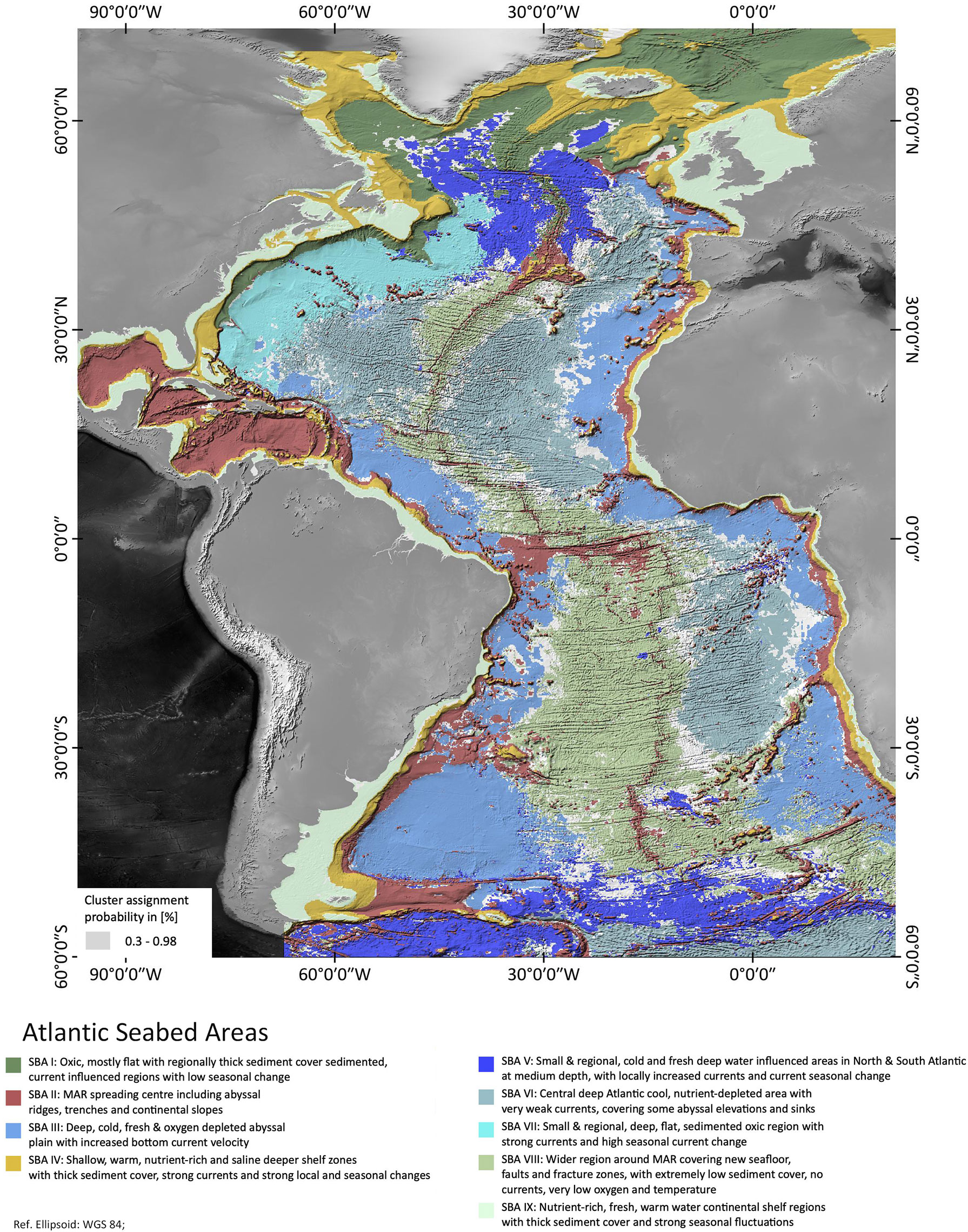
Figure 1 Atlantic Seabed Areas as identified by the Gaussian Mixture Model analysis along with cluster probabilities. Areas of saturated colors have a probability of >98% of being classified correctly. Especially at the cluster boundaries, probability decreases.
To understand what distinguishes the SBAs and what are the dominating factors, a look at the boxplots below is of use (Figure 2). They give quantitative information, outlining the characteristics of each cluster and indicating which parameter describes the respective cluster in the first order. The boxes contain 50% of the data. The ‘whiskers’ (straight lines below and above the box) denote minimum and maximum data values, respectively, such that box and whiskers include 95% of the data. The larger the box, the wider is the value span or variation of the respective input variable across a cluster. The median (central horizontal line inside the box) is another important measure when interpreting boxplots. It shows the middle quartile of the data set and, opposite to the mean or average, it is not sensitive to outliers. A mean value (dot inside the box) that is far away from the median indicates a bias towards the direction of displacement. The most illustrative boxplots are presented below (Figure 2). The complete set of boxplots for all input variables can be found in the Supplementary Material F1. A summary of the cluster statistics is listed in Tables A1, A2 of the supplementary material. A detailed boxplot assessment and boxplots including extreme values are given in the Supplementary Material F2, T1.
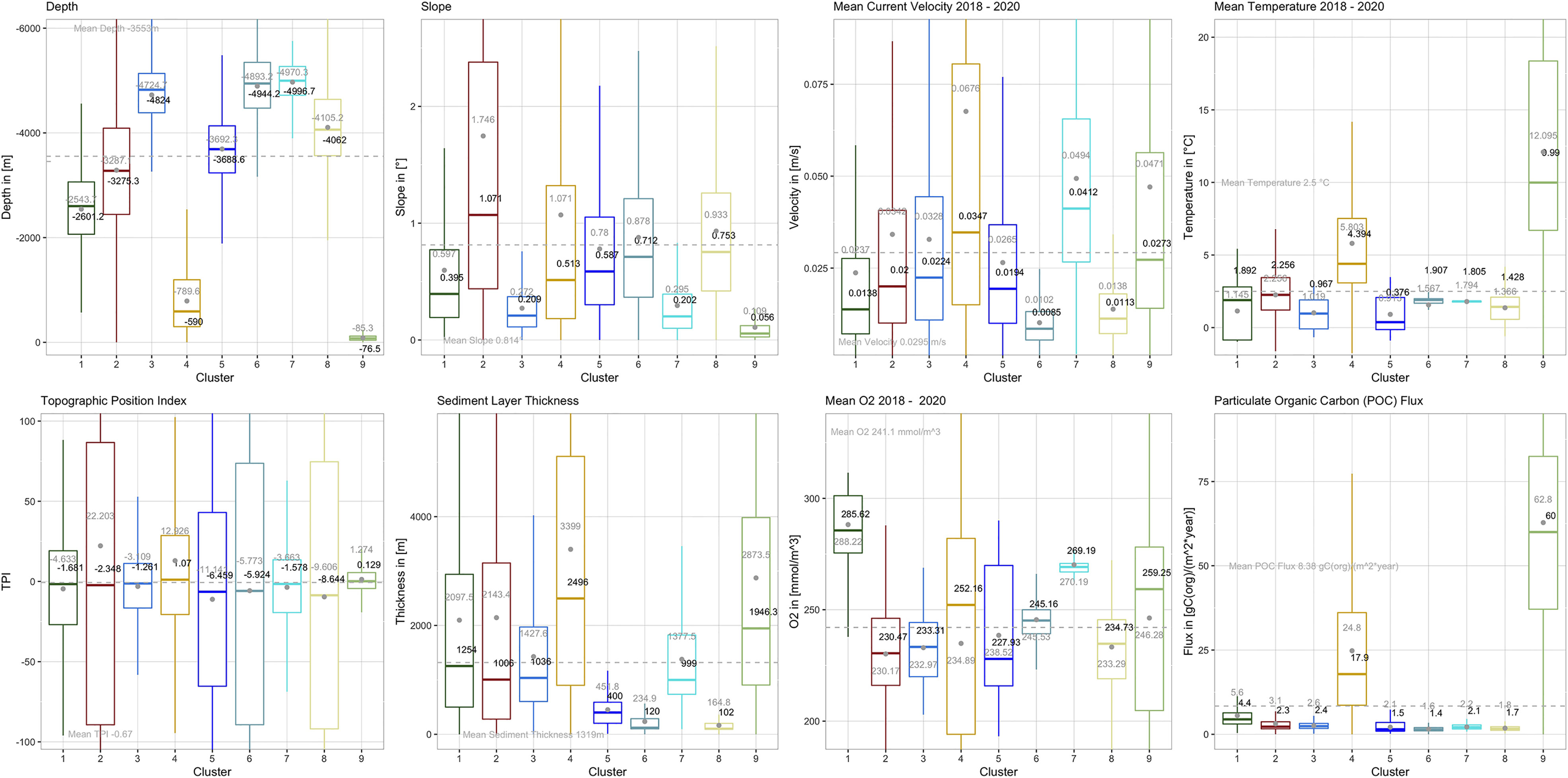
Figure 2 Boxplots outlining the SBA characteristics. The boxes comprise the groups’ interquartile ranges, i.e. between the upper (75%) and lower (25%) quartiles and contain the central 50% of the data. The ‘whiskers’ (straight lines below and above the box) denote minimum and maximum data values, and together with the boxes make up 95% of the data set. The remaining 5% are extreme values, which for better visibility are not shown here. They can be found in boxplots of the supplementary material F2. The colored lines/grey dots inside the boxes indicates the groups’ median/mean, whereas the grey dashed line is the overall data set’s median.
Although we see from the box-plots that there is seldom a single environmental variable that describes a particular SBA, we can make some general statements about their most defining characteristics. Table 1 presents a short outline along with the area covered by each SBA.
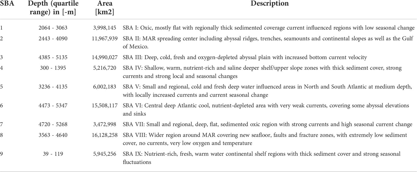
Table 1 SBA description summary ordered by area covered (from smallest to largest).
3.1 Cluster probability
As the clustering is based on the probability of any one 1/12°x1/12° cell being classified into one of the nine SBAs, a ‘hard boundary’ - map showing all cells in the colour corresponding to their most probable cluster could be misleading if many cells had quite similar probabilities for a number of clusters. To test how robust the classification is, we examined the absolute values of the dominant cluster probability, hereafter referred to as probability. A cumulative curve of the classification probabilities [plotted as “probability = 1 – uncertainty” as of Fraley & Raftery (2003)] is shown in Figure 3. On Figure 1, the grey colours illustrate probabilities of less than 98%, those were excluded. We see from Figure 3 that more than 85% of the cells are assigned to a dominant cluster with a probability of > 95% (uncertainty < 0.05). Only around 2% of the cells lie in a transition zone of 40-60% probability. Figure 1 shows that these higher-uncertainty cells mainly lie at SBA boundaries, presumably reflecting the regions where environmental variables are in transition between one SBA and another. The cells which are classified with 0 uncertainty generally lie in the centre of an SBA patch, classified as belonging to just one SBA.
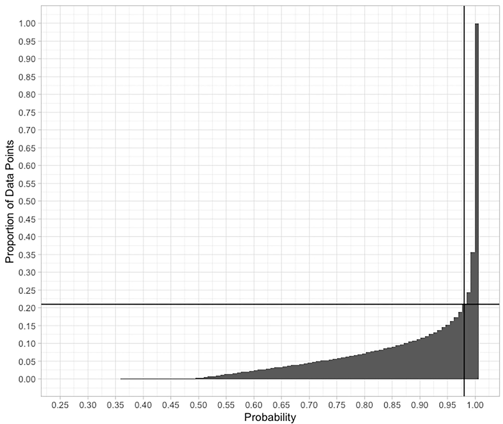
Figure 3 A plot of cumulative frequency of observed probabilities in the classification of individual grid cells into one of the nine SBAs. The lines indicate the 98% probability threshold that includes 79% of the data. Over 85% of the cells are classified with > 95% certainty.
3.2 Landscape diversity
To highlight the diversity of the Atlantic sea floor landscape, we ran a moving window analysis based on landscape ecology principles (e.g. Swanborn et al., 2022) that automatically identifies areas where several cluster boundaries meet. Regions of high diversity are at the same time those with the highest classification uncertainties. To be confident that our search for areas of high landscape diversity is not weakened by these poorly-classified cells, we included only points with classification probabilities of >= 98% in the analysis. This still amounted to about 80% of the data but significantly reduced the data density in cluster boundary regions.
The diversity analysis was executed using the package ‘landscapemetrics’ (Hesselbarth et al., 2019). A major part of it is based on FRAGSTATS (McGarigal et al., 2012), a program that automatically quantifies landscape structure and has been implemented in R by Hesselbarth et al. (2019). In combination with a moving window, we used patch richness (PR) index, a simple diversity indicator that counts the number of different patch types within a given area (McGarigal et al., 2012). A patch describes the local area covered by a single SBA: Hence, the more patches of different SBAs in an area, the higher the PR and local diversity. As we did not want to fix patch sizes in advance by defining a search radius, we chose a cell-wise moving window approach with a window size of 3x3, including only one cell and its direct neighbours. This approach catches even the smallest region of high diversity. The PR index expresses the numbers of different neighbours of a cell, with a minimum to maximum count of one to four neighbours.
Figure 4 is a heatmap showing the patch richness as a result of the diversity analysis. Regions of large densities of high SBA diversity are highlighted as indicated by the red colours. The highlights must be understood as a count of the different neighbours per area – the more cells with a high number of different neighbours in a region, the more intense the yellow/red colour. The highlighted areas are well spread across the central Atlantic basin, less in the Northern Atlantic. They correspond in parts with the latest EBSAs as defined by the Convention of Biological Diversity (CBD) 2019. Most of them are associated with and around SBA II, which is the sparsest of all SBAs, hence with most cluster boundaries. Many of the highlights are found around small-scaled patches. Only few are in the vicinity of one large patch of a single SBA, which is why in the region > 55°, where large patches prevail, there is less patch diversity. We chose two regions on Figure 5 for a detailed inspection to highlight what this patch richness means in terms of landscape variability.
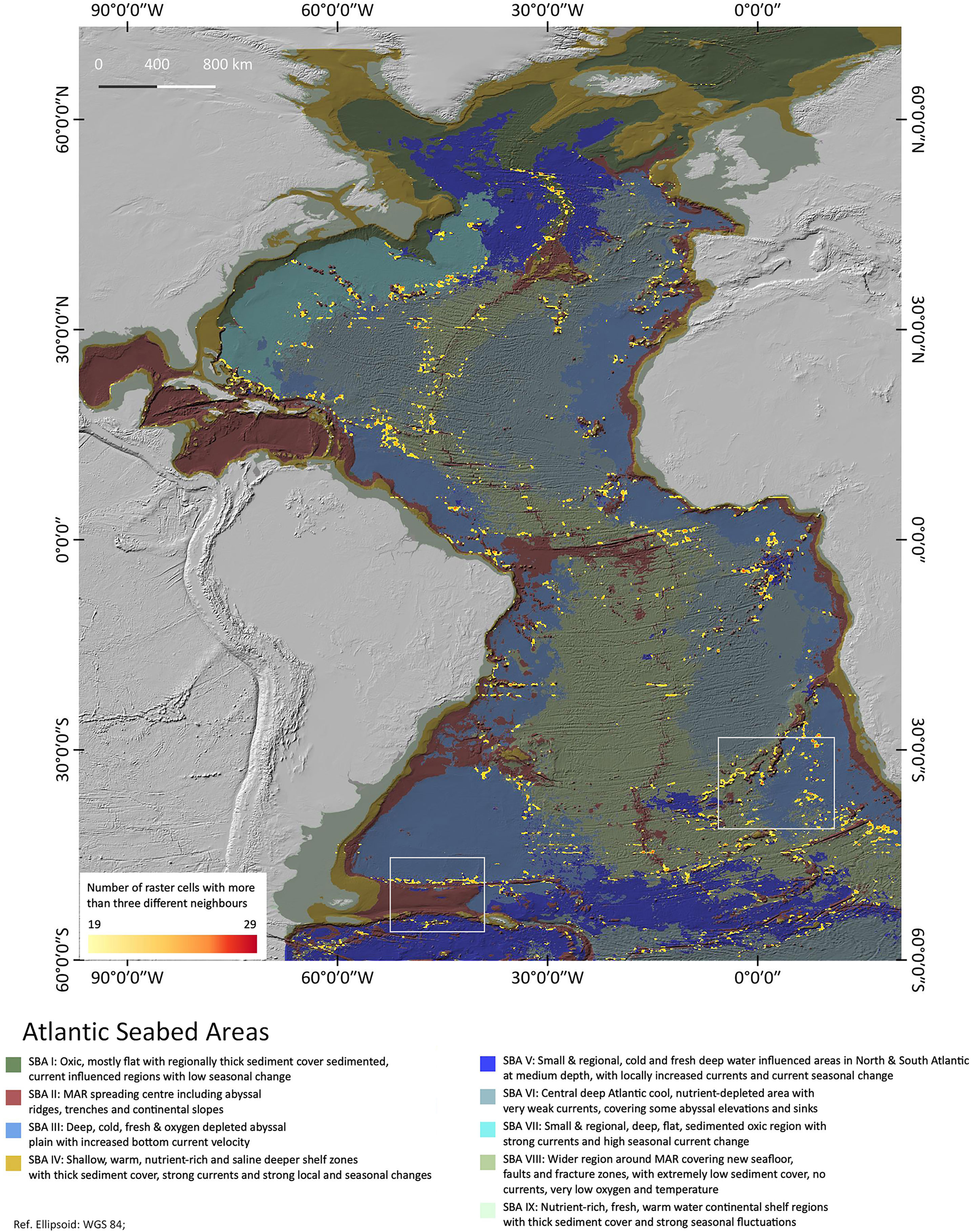
Figure 4 Atlantic Seabed Area diversity density. A patch richness analysis map highlighting areas of high SBA diversity. The boxed areas of Walvis ridge and Falkland Plateau are discussed in more detail below in Figures 5 and Figure 6.
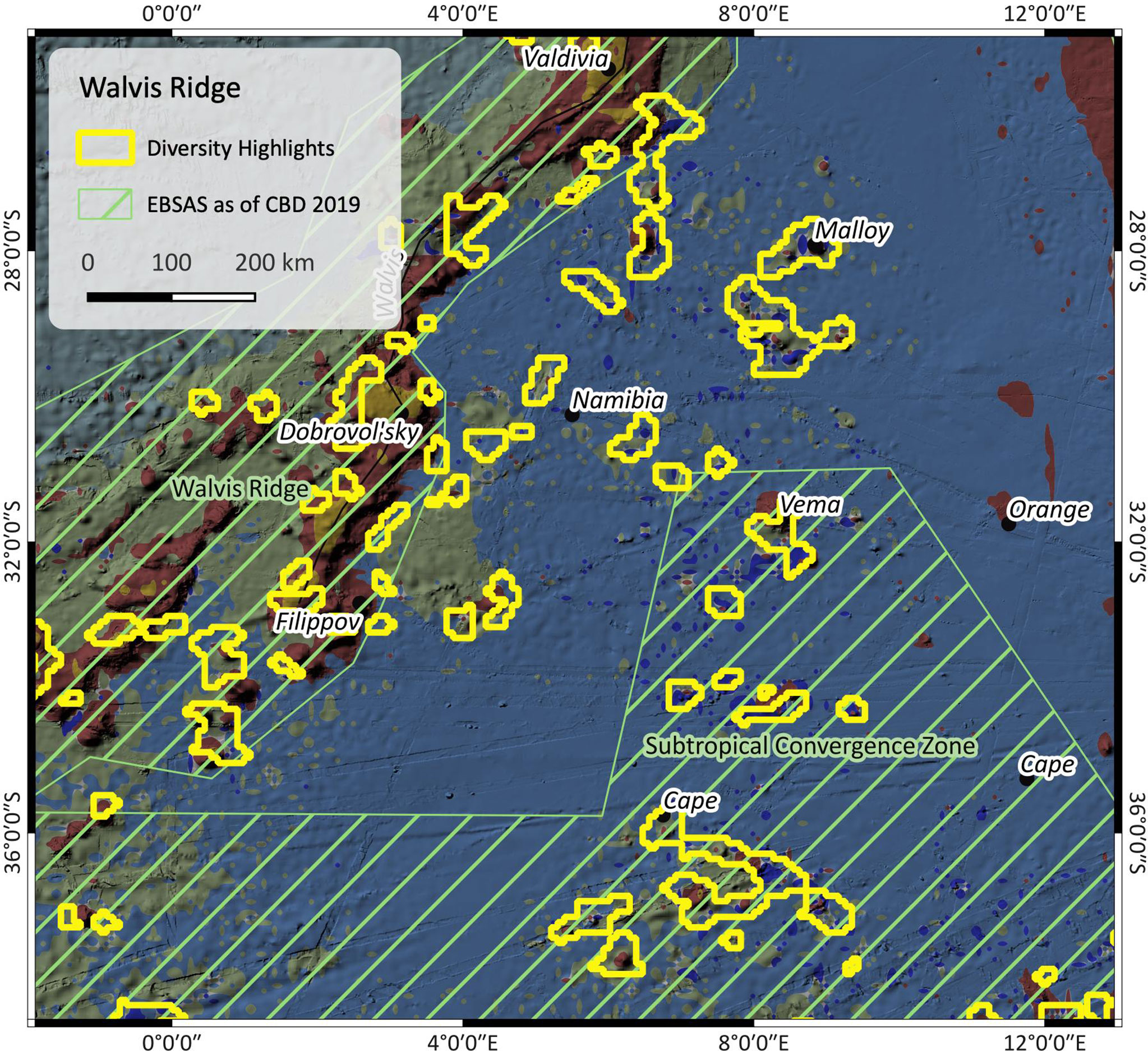
Figure 5 Patch richness near Walvis ridge. The outlines are the highlighted regions as found by the patch richness analysis. The map also shows EBSAs (green stripes) as of CBD 2019. For SBA color legend, please refer to Figure 1.
Figure 5 shows the Namibia abyssal plain and Cape Basin, as well as the southern edge of Walvis ridge, with red outlines indicating regions of high SBA diversity. SBA III prevails, along with several patches of SBA VII and seamounts covered by SBA II. Besides the presence of seamounts, the input data suggest deep and cold abyssal plain under the influence of strong currents. The oxygen is slightly higher within the Walvis ridge EBSA than in the Subtropical Convergence Zone EBSA and the Namibian abyssal plain in between. Also, currents are locally stronger, e.g. south of the Walvis ridge line and weaker in the deeper basin. Here, the highlighted areas along Walvis ridge correspond to the Walvis Ridge EBSA patch, but not so well to the Subtropical Convergence Zone EBSA further south.
Figure 6 shows the Falkland escarpment north of the Falkland plateau and the Tehuelche fracture zone south of the plateau. At the escarpment, the highlights mainly include SBAs II & III and some small patches of SBA V. At Tehuelche fracture zone, these are SBAs II, V and VIII. The input data indicate higher current speeds and increased seasonal change north than south of the plateau and especially along the Falkland escarpment which can be associated with the influence of the Malvinas current and the Argentine gyre (Yu et al., 2018).
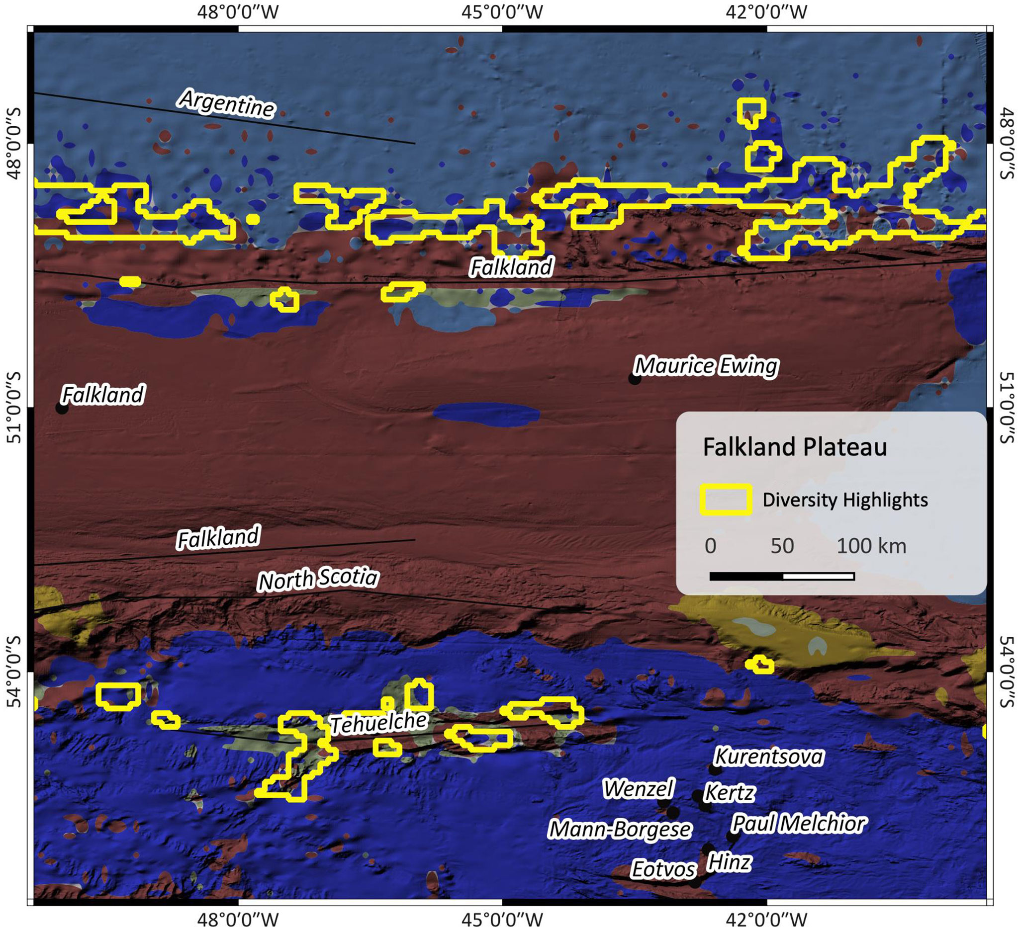
Figure 6 Patch richness at Falkland fracture Zone. The outlines are the highlighted regions as found by the patch richness analysis. For SBA color legend, please refer to Figure 1.
4 Discussion
4.1 How the SBAs relate to existing data and publications
The unsupervised clustering of the Atlantic seabed environment resulted in nine seabed areas, with characteristics summarised in Table 1. To interpret the SBAs, we compared them to published oceanographic patterns such as large currents, upwelling systems and water-mass formation zones as well as to predicted seamounts (Yesson et al., 2011a; Yesson et al., 2011b), and hydrothermal vent locations (Beaulieu and Szafrański, 2020). Many of the SBAs are influenced by currents, water masses and water formation zones. A striking example for this is SBA VII which is confined to one region: the major spreading path of NADW through the North Atlantic deep abyssal plain (e.g. Gary et al., 2011). High oxygen concentrations, cold water, very strong currents and high seasonal change support the interpretation as a highly ventilated region (Figure 1 in Rahmstorf, 2006). The partitioning into a Northern and a Southern compartment of SBA V can be related to the influence of Labrador Sea Water (LSW) formation taking place in the deep convection zone of the Labrador basin (Koelling et al., 2022), which spreads out into the central Atlantic Ocean as part of the North Atlantic Deep Water (NADW), as well as to Antarctic Bottom Water (AABW) in the Weddell Sea (Figure 1 in Rahmstorf, 2006). This is underpinned by the expert knowledge-based GOODS classification whose authors found a strong division into North and South Atlantic, too (Supplementary Material Table T4, IOC, 2009; Morato et al., 2021).
SBA IV encloses the Atlantic’s deeper shelf zones and regions of strong local (boundary) current systems with a high seasonal variability, such as the East Greenland current or overflow areas such as the Greenland-Scotland-ridge complex (Mauritzen, 1996; Rahmstorf, 2006; Våge et al., 2011; Semper et al., 2020). Similar to this but in shallower regions is SBA I, strongly influenced by water formation zones in the Labrador and Greenland Sea as well as by the boundary and overflow currents. SBAs I, IV and VII show an increased oxygen concentration, emphasising the influence of mixing processes. Lower oxygen concentrations in moderate depths (SBA V) may be attributed to enhanced biological productivity (e.g. (Sigman and Hain, 2012; Schmidtko et al., 2017), oxygen depletion during the spreading of water masses, like e.g. the AABW on its way up North (Menezes et al., 2017) or oxygen minimum or even dead zones (Diaz et al., 2013; Rabalais, 2021). SBA II sticks out as it seems to be mainly defined by topography, covering areas of rough terrain and corresponding well with the spreading center of the MAR. It is the patchiest of all SBAs. In major parts, SBA II agrees with listed hydrothermal vent fields (Beaulieu & Szafrański, 2020) and seamounts (Yesson et al., 2011a; Yesson et al., 2011b).
4.2 Comments on the seascapes, GOODS and EMUs
We further compared the SBAs to the seascapes described by Harris and Whiteway (2009), to the GOODS biogeographic provinces (IOC, 2009) and to the Ecological Marine Units (‘EMUs’) found by Sayre et al. (2017). The latter have also been used by Morato et al. (2021) to assess their suitability for a species distribution model (SDM). Harris and Whiteway (2009) used a clustering approach (isoclass) on seafloor data which is most similar to ours. Sayre et al. (2017) also used a similar technique (KMeans), applied in 3D on the water column. Their EMUs are three-dimensional entities, vertically comprising water column layers rather than separating the seafloor from the water body above which makes it difficult to directly compare to our seafloor-only zones. The same applies to GOODS, which moreover is purely expert-based and hence subjective. Table A3 in the supplementary material lists the SBAs we found against the classes of Harris and Whiteway (2009), Sayre et al. (2017) and GOODS to give an approximate conversion. Also, only major matching areas are included; those that have minor overlap are left out to avoid confusion. In Table A4, the input parameters and methods of all aforementioned classifications are listed.
When comparing the SBAs we identified to the seascapes by Harris & Whiteway (2009), some (esp. SBAs III, V, VII) can be ‘translated’ into one single seascape (10), others (e.g. SBA VIII) correspond to more than one seascape (5, 7 and 9). This might be because we used additional non-morphologic parameters like current speed, POC flux, etc., higher resolution data (1/12° for SBAs, 1/10° for seascapes), and more recent data. We have not included primary production in the classification, as it is a variable mostly determining the ocean surface and the upper water column until a depth of around -350 m (CMEMS, 2021). Instead, we used POC flux to the sea floor. On the other hand, Harris and Whiteway (2009) did not take into account seasonal variability, a measure we considered crucial for currents, salinity, temperature, and oxygen concentration. They further excluded salinity, arguing that its variation at seafloor depths is very low. This may be correct in the deeper parts of the Atlantic, but our results show that salinity values and seasonal variability do play a role, for example, in the shallower SBA IX region, a region that was excluded on their seascape map. In addition, the seascapes of Harris & Whiteway (2009) were defined on a global scale and, depending on the principal parameters that defined the respective seascape, those may have varied across the global ocean compared to the Atlantic basin. Another difference is that we applied a different clustering technique, one which allows for cluster shapes other than only spherical.
The other two mentioned classifications GOODS (IOC, 2009) and EMU (Sayre et al. (2017)) follow different approaches: GOODS is a purely expert-based (subjective) classification without automated or computer-based process. EMUs are three-dimensional entities, vertically comprising water column layers rather than separating the sea floor from the water body above.
The non – comparability of marine classifications is, according to Lecours (2017), a significant drawback regarding their use. Table A3 in the supplementary material shows that, except for the smaller SBAs I and VII, all SBAs correspond to more than one biogeographic region. As both EMUs and the GOODS areas have a large extent, several of those regions are almost as large as the entire Atlantic basin. Nevertheless, in marine spatial planning or MPA network designation processes, for example, it might be extremely useful to consult more than one classification to illuminate several aspects of the same area (e.g. Lecours et al., 2017).
The use of ocean landscape maps with regard to conservation targeted decision making is pointed out by Lecours (2017) as being somewhat like the classic problem of comparing apples and pears: There is a lack of uniformity concerning input data selection, standardised clustering techniques and algorithms. Furthermore, quality assessment widely differs and there is no method yet to combine the uncertainties and errors that occur during a mapping process into one ultimate uncertainty estimation. Visualising mapping results in e.g. interactive GIS is a first step to tackle those challenges, but in the long run, standardising determining variables, methods and error estimation might become inevitable (Lecours 2017).
4.3 Seabed areas and marine life
It is difficult to state whether the environmental clusters identified here contain distinct species assemblages: in addition to physical conditions, life-history traits and biological interactions will influence biogeographic patterns. Even if the physical environment is similar, species and assemblages may differ.
While individuals may not be the same, species with similar traits and functional behaviour could populate areas with comparable physical environments (e.g., burrowing fauna in heavily sedimented areas or filter-feeders in complex, rocky environments) (e.g. McGill et al., 2006; Zeng et al., 2020). From a biodiversity management perspective, such spatially explicit delineation of potential ecosystem functions (and therefore services) is of high value even if the exact species occupying the particular environment are not known. Quantitative metrics like the patch richness index to calculate diversity can discover those regions automatically and objectively.
Morato et al. (2021) have made steps towards integrating biogeographic province maps into environmental niche modelling (e.g. species distribution models (SDM) or habitat suitability models (HSM)). In their work, they compare the two seafloor bioregion models EMU and GOODS to an SDM. Although their results show only very little to hardly any agreement of the SDM’s with the bioregions’ boundaries, they still outline a valuable approach and a possibility of implementing those kinds of classifications into species prediction related work. Nevertheless, to effectively predict and relate species to environmental conditions, classifications and data at a finer scale must be available (Lim et al., 2021). The combination of high-resolution classifications and SDMs or HSMs is a very promising task, capable of supporting marine area-based management and spatial planning work (Lim et al., 2021; Morato et al., 2021).
At the same time, it is crucial to keep in mind that the map presented here is based on the current environmental conditions. As a result of climate change, seabed environments will change (e.g. rising temperatures, reducing oxygen content of the bottom waters), and so may the SBAs. The SBAs may change in shape and extent, or in characteristics. A next step may be to create similar marine landscape maps based on future predictions of the seafloor environment under different climate scenarios, in order to provide policy-makers with a forward look in addition to the comprehensive description of the present-day situation presented here.
4.4 Automatically finding areas of interest - interpretation of the patch richness analysis in relation to EBSAs
The results of such patch richness analyses ought to make it easier to identify potential areas of interest. Because they are based on a multivariate cluster analysis, they combine complex ensembles of multiple influencing parameters, a process which is challenging for a human brain but simple for machine algorithms. The highlights shall draw our attention to areas where special conditions prevail, and which might be worth to have a closer look at. In the case of the Falkland region (Figure 6), the Falkland plateau seems to be a barrier between two areas that are under the influence of different variables as shown by the altered composition of neighbouring SBAs. The highlights in Figure 5 mostly cover seamounts or other subsea features, which, with regard to the Walvis Ridge where highlights and EBSA largely correspond, confirms that this is an area of significance.
From Figures 4–6, we see that landscape diversity hotspots are often found on and around seamounts or regions of strongly varying topography. This is perhaps not surprising as they are the regions where the physico-chemical conditions in the ocean are known to change significantly over small spatio-temporal extents. It is for this reason that research has often been concentrated there (e.g. Clark et al., 2011). Over the Atlantic basin, the identified regions of high landscape diversity correspond in parts with the latest EBSAs. As EBSAs need a certain amount of ground-truth data for their definition, our landscape diversity map could be useful to concentrate research in presently unstudied areas which may harbour significant landscape diversity.
EBSAs are defined on a solid data basis which is why there may be a bias towards well investigated regions. This may be the fact in the Walvis ridge region (Figure 5) – with Walvis ridge itself being significantly more examined than the surrounding environment. The EBSA patch covers the entire Walvis ridge and the area around Cape basin but only some of the nearby seamounts – besides other reasons probably due to insufficient existing data. It is not easy to find proof for this assumption. A search in Google scholar in April 2022 however yields over 300 hits for publications containing Walvis Ridge in their title, over 500 containing Cape basin and 25 for Vema seamount, but none for e.g. Malloy seamount. This could be an indicator for unbalanced data distribution and research effort between these areas.
Furthermore, EBSA definition is based on multiple criteria where (biological) diversity is just one of them. In addition to the sea floor, the water column is taken into consideration, too. It is hence obvious, that the EBSAs only partially agree with the highlights: For example in areas like the Labrador Sea, whose sea floor is defined by only one SBA, the water column however is highly dynamic due to deep water convection, making it a unique spot and EBSA candidate (CBD 2021). On the other hand, there are numerous highlights that are not within existing EBSAs or MPAs, like e.g. in the basins of Guiana or Newfoundland. This might be due to a lack of ground truth data needed for EBSA designation. It may also be because some regions we highlighted fail on other EBSA criteria. It has to be noted, though, that currently, some regions still lack EBSA expert workshops and do hence not have any EBSAs at all, like e.g. the Argentine basin. Also, to date, the North-East Atlantic most recent EBSAs have not been published yet, so there is a lack of coverage here, too. Nevertheless, the highlights of diversity in combination with the SBA map pinpoint towards regions of interest and can help finding and defining new research areas, e.g. to support cruise proposals or contribute to marine protection-based decision making, regarding location and extent of potential MPAs or new EBSAs. They may be able to support entire stages of EBSA identification without introducing too much subjectivity.
Methodological constraints, potential errors and data limitation
Despite the fact that multivariate clustering techniques are more objective than hierarchical methods, unsupervised analyses can still bear error sources that may not be visible at first sight but must be considered when using them.
Resolution
Although a density estimation and model-based clustering approach seems suitable for this kind of high dimensional and complex data, it is the input data quality that needs to be looked at. The most prominent quality-reducing factors are differences in resolution, especially when dealing with multiple data sources. This holds true for vertical as well as for horizontal resolution. At depths > 1000 m, CMEMS model data products have a very low vertical resolution of about 450 m (Lellouche et al., 2019). Hence, they only give a very rough approximation of the conditions prevailing in those depths or at the seafloor. Local small-scale (vertical) variations (e.g., in temperature, caused, for example, by hydrothermal vent fields) or the few-meters thick bottom boundary layer will not be resolved. Given that ground truth seafloor data are scarce in the deep sea, we considered for our analysis the last depth level as defined by CMEMS to be representing seafloor conditions. This induces a huge vertical uncertainty, which cannot be resolved with the present data and models. Bathymetry, on the other hand, is a seafloor layer by nature, and can have a much higher vertical resolution. Tozer et al. (2019a) state +/- 150m for the satellite data, but e.g. bathymetry acquired from multibeam systems may reach an order of metres to tens of metres. Hence in places, we are aligning data from nominally different depths: those directly at the seafloor (e.g., bathymetry), and the others in a vertical range between seafloor level and 450 m above it (CMEMS model data).
Horizontal resolution is another constraint and mainly attributed to limited data availability. For this analysis, we re-sampled all data layers to the CMEMS physical data product resolution of 1/12° (around 8 km at the equator (Lellouche et al., 2019)), which required downscaling the CMEMS biological product and upscaling the bathymetry data. Another option would have been to upscale all data to the lowest resolution, which in this case was ¼° (of the CMEMS biological product). However, we dismissed this option, as the information loss would have been intolerably high considering the fact that oxygen and phytoplankton are the only data of this low resolution. Notably, even 1/12°, or 8 km, is a very coarse scale which does not resolve small scale variations or features that might be of importance, like e.g. submarine volcanoes or small oxygen dead zones. Local hydrodynamic and morphologic conditions are important drivers for food flux and organic matter transport to the seabed. These processes however typically operate at the scale of an offshore bank or seamount, i.e. at a resolution of maximum several hundreds of metres, and might hence not captured within this study.
Both downscaling from low to high resolution as well as the reverse can be critical; this is because high-resolution data naturally inherit more parameter variance that is passed on when resampled to coarser resolution than data that was collected at a coarse resolution in the first place, thus affecting the analysis. To at least partially accommodate this in our analysis, we scaled the data and chose model-based clustering, as it is robust towards different variances (e.g., Scrucca et al., 2016).
An approach to obviate these deficiencies could be using nested classifications, running multiple cluster algorithms on the existing classes as performed in Hogg et al. (2016). This would refine the original clusters and split them into smaller parts, but would, of course, not change the initial data resolution. Such nesting of classifications, on an ocean basin scale, would however result in complex clusters with multiple hierarchical levels which would be unwieldy to analyse.
Higher resolution ocean models (e.g. VIKING20X (Biastoch et al., 2021) or INALT (Schwarzkopf et al., 2019)), if available down to the km-scale on a basin-wide or even global scale, would significantly improve this kind of seabed clustering. To date, such models usually have a very fine resolution at the sea surface which also becomes coarse towards the seafloor. In our approach we preferred the CMEMS product, even though it has the same limited vertical resolution at depth. However, because CMEMS used an assimilation towards observational data (despite the fact that these are sparse at depth) we aimed at a more realistic representation of the hydrography.
Variable selection
Another limitation which may influence the classification result is the predictor variable selection itself. This issue has been widely discussed (e.g., Harris and Whiteway, 2009; Howell, 2010; Watling et al., 2013) and several determinants have been agreed as being good representatives of the ocean environment. In this study, we focussed on morphological and hydrographical parameters, largely leaving out biologic measures, as our aim was to define submarine landscapes (e.g. Pearman et al., 2020). However, the ocean and its inhabitants form a coherent system and likewise, human impacts (e.g., mining, fishing, etc.) have a severe influence on these ecosystems. Hence, in the future data selection will have to be expanded to encompass the full range of factors that affect the seafloor habitat. A more holistic approach, also with respect to marine protected area designation, would not only be to include a larger span of environmental data, but also information on natural resources abundances, fishing grounds, etc., such as bottom-trawling fishing activities that negatively impact the benthic environment (Eggleton et al., 2018; Ferguson et al., 2020). Visalli et al., 2020 for example worked out a data-driven spatial planning tool aiming to highlight priority regions in the ABNJ for protection. For the whole-Atlantic approach targeted here, the data layers necessary for this extended type of analysis are, sadly, simply not available at present.
Conclusion
This work presents a marine landscape map of the Atlantic seafloor based on an unsupervised, multivariate statistics cluster analysis. We found nine seabed areas in total, each of them being unique and differently defined by oceanographic and morphologic determinants. Unsupervised cluster analyses have the advantage of providing an objective view on the ocean environment, stepping away from human-defined hierarchical categorisations towards an unbiased understanding of seafloor ecosystem coherence.
Generally, depending on the clustering technique applied and the selection of input parameters, the results can be very different, highlighting the complexity and variability of the ocean. As there is not the one ‘true’ arrangement of marine bio-physio-chemical-morphologic regimes, verification can only take place via ground truthing – and even this may not catch the entire complex diversity. Hence, depending on the purpose, a combination of several existing models may be more useful than one single classification. Automated landscape analyses can help to understand the classifications better, and subsequent quantitative metrics will help to identify biodiversity hotspots and vulnerable habitats by pointing out new complex regions of interest. Studies like this and in combination with other, also smaller-scaled classifications can be used e.g. for protection-targeted decision making. Our SBAs for example have been implemented into the designation process for the new NACES MPA and acts as one of the knowledge bases to the local prevailing conditions.
A valuable future task would be to assess whether species distribution patterns can be further related to the SBAs we found. Also collating more ground truth data and a detailed assessment of the diversity highlighted regions shall support decisions about protection objectives.
Data availability statement
Publicly available datasets were analyzed in this study. This data can be found here: World data Service for Geophysics: https://ngdc.noaa.gov/mgg/sedthick/, Copernicus Marine Data Service: https://resources.marine.copernicus.eu/products, Shuttle Radar Topography Mission/Opentopography: https://opentopography.org. The resulting cluster shape file can be found here: https://doi.pangaea.de/10.1594/PANGAEA.946690: or directly under: http://www.geonode.iatlantic.eu/layers/geonode:AtlanticSeabedAreas_WGS84.
Author contributions
MS, VH, CD, AB, and PM contributed to conception and design of the study. MS, PM, AB, and SM organized the data and performed the statistical analysis. MS prepared the figures and wrote the first draft of the manuscript. VH and CD wrote sections of the manuscript. AB gave input to oceanic models and error analysis and CD gave input to the use of the analysis. All authors contributed to manuscript revision, read, and approved the submitted version.
Funding
This work was supported by the iAtlantic project, funded by EU/HORIZON 2020, Blue Growth (grant agreement No 818123). The results are hosted on the iAtlantic Geonode (geonode.iatlantic.eu/). The authors owe gratitude to the oceanography group at GEOMAR, Helmholtz Centre for Ocean Research, for providing help with oceanographic model know-how.
Acknowledgments
Special thanks to Iason Gazis from Geomar for their help during the process of clustering model selection. We are further grateful to Catherine Wardell from National Oceanography Centre and to Anne-Cathrin Wölfl form GEOMAR for support in R scripting. We would also like to thank the reviewers for their valuable and friendly comments and their support.
Conflict of interest
Author SM was employed by the company Briese Schiffahrts GmbH & Co.
The remaining authors declare that the research was conducted in the absence of any commercial or financial relationships that could be construed as a potential conflict of interest.
Publisher’s note
All claims expressed in this article are solely those of the authors and do not necessarily represent those of their affiliated organizations, or those of the publisher, the editors and the reviewers. Any product that may be evaluated in this article, or claim that may be made by its manufacturer, is not guaranteed or endorsed by the publisher.
Supplementary material
The Supplementary Material for this article can be found online at: https://www.frontiersin.org/articles/10.3389/fmars.2022.936095/full#supplementary-material
References
Aumont O., Ethé C., Tagliabue A., Bopp L., Gehlen M. (2015). PISCES-v2: an ocean biogeochemical model for carbon and ecosystem studies. Geoscientific Model. Dev.8, 2465–2513. doi: 10.5194/gmd-8-2465-2015
Beaulieu S. E., Szafrański K. M. (2020). InterRidge global database of active submarine hydrothermal vent fields version 3.4 (www.pangaea.de). doi: 10.1594/PANGAEA.917894
Biastoch A., Schwarzkopf F. U., Getzlaff K., Rühs S., Martin T., Scheinert M., et al. (2021). Regional imprints of changes in the Atlantic meridional overturning circulation in the eddy-rich ocean model VIKING20X. Ocean. Sci.17, 1177–1211. doi: 10.5194/os-17-1177-2021
Brewer C., Harrower M. (2021) ColourBrewer, the Pennsylvania state university. Available at: https://colorbrewer2.org/ (Accessed August 2021).
British Oceanographic Data Centre (2020) Gebco gridded global bathymetry data. Available at: https://www.gebco.net/data_and_products/gridded_bathymetry_data/gebco_2020/ (Accessed August 2021).
CBD Secretariat (2009). “Azores Scientific criteria and guidance,” in For identifying ecologically or biologically significant marine areas and designing representative networks of marine protected areas in open ocean waters and deep sea habitats. CBD: Secretariat of the Convention on Biological Diversity:Montreal, Canada
Convention on Biological Diversity (CBD) Secretariat. (2021) Ecologically or biologically significant marine areas - special places in the world's oceans. Available at: https://www.cbd.int/ebsa/ (Accessed March 2022).
Chune S. L., Nouel L., Fernandez E., Derval C., Tressol M., Dussurget R. (2020). Product user manual for global biogeochemical analysis and forecast product GLOBAL_ANALYSIS_FORECAST_PHY_001_024. EC Copernicus marine environment monitoring service 1.6. 34 Copernicus Marine Environment Monitoring Service, implemented by Mercator Ocean International (MOi):Toulouse, France, Public Ref.: CMEMS-GLO-PUM-001-024.
Clark M. R., Consalvey M., Rowden A. A. (2016). Biological sampling in the deep Sea. 1. Edition (New York:John Wiley & Sons), 472 Pages. doi: 10.1002/9781118332535
Clark M. R., Watling L., Rowden A. A., Guinotte J. M., Smith C. R. (2011). A global seamount classification to aid the scientific design of marine protected area networks. Ocean Coast. Manage.54, 19–36. doi: 10.1016/j.ocecoaman.2010.10.006
Combes M., Vaz S., Grehan A., Morato T., Arnaud-Haond S., Dominguez-Carrió C., et al. (2021). Systematic conservation planning at an ocean basin scale: Identifying a viable network of deep-Sea protected areas in the north Atlantic and the Mediterranean. Front. Mar. Sci.8. doi: 10.3389/fmars.2021.611358
Davies C. E., Moss D., Hill M. O. (2004). EUNIS habitat classification revised 2004 (Paris: European Topic Centre on Nature Protection and Biodiversity), 127–143. Available at: http://eunis.eea.europa.eu/upload/EUNIS_2004_report.pdf.
Diaz R. J., Eriksson-Hägg H., Rosenberg R. (2013). “Chapter 4 – hypoxia,” in Managing ocean environments in a changing climate. Eds. Noone K. J., Sumaila U. R., Diaz R. J. (Burlington MA, USA:Elsevier Inc.,), 67–96. doi: 10.1016/B978-0-12-407668-6.00004-5
Eggleton J. D., Depestele J., Kenny A. J., Bolam S. G., Garcia C. (2018). How benthic habitats and bottom trawling affect trait composition in the diet of seven demersal and benthivorous fish species in the north Sea. J. Sea Res.142, 132–146. doi: 10.1016/j.seares.2018.09.013
EU Copernicus Marine ServiceOperational Mercator biochemical global ocean analysis and forecast system, GLOBAL_ANALYSIS_FORECAST_BIO_001_028. Available at: https://resources.marine.copernicus.eu/?option=com_csw&view=details&product_id=GLOBAL_ANALYSIS_FORECAST_BIO_001_028 (Accessed February 2021).
EU Copernicus Marine ServiceOperational Mercator global ocean analysis and forecast system, GLOBAL_ANALYSIS_FORECAST_PHYS_001_024. Available at: https://marine.copernicus.eu/node/173 (Accessed February 2021).
Ferguson A. J. P., Oakes J., Eyre B. D. (2020). Bottom trawling reduces benthic denitrification and has the potential to influence the global nitrogen cycle. Limnol. Oceanog.5, 237–245. doi: 10.1002/lol2.10150
Fraley C., Raftery A. E. (2003). SOFTWARE REVIEW: Enhanced model-based clustering, density estimation, and discriminant analysis software: MCLUST. J. Classification20, 263–286. doi: 10.1007/s00357-003-0015-3
Gary S. F., Lozier M. S., Böning C. W., Biastoch A. (2011). Deciphering the pathways for the deep limb of the meridional overturning circulation. Deep Sea Res. Part II58, 1781–1797. doi: 10.1016/j.dsr2.2010.10.059
GDAL/OGR contributors (2021) GDAL/OGR geospatial data abstraction software library (Open Source Geospatial Foundation). Available at: https://gdal.org (Accessed August 2021).
Gille S. T., Metzger E. J., Tokmakian R. (2004). Seafloor topography and ocean circulation. Oceanography17. doi: 10.5670/oceanog.2004.66
Harris P. T., MacMillan-Lawler M., Rupp J., Baker E. K. (2014). Geomorphology of the oceans. Mar. Geology352, 4–24. doi: 10.1016/j.margeo.2014.01.011
Harris P. T., Whiteway T. (2009). High seas marine protected areas: Benthic environmental conservation priorities from a GIS analysis of global ocean biophysical data. Ocean Coast. Manage.52, 22–38. doi: 10.1016/j.ocecoaman.2008.09.009
Hastie T. J., Tibshirani R. J., Friedman J. H. (2001). “The elements of statistical learning: data mining, inference, and prediction,” in Springer series in statistics (New York, New York, USA: Springer).
Hesselbarth M. H. K., Sciaini M., With K. A., Wiegand K., Nowosad J. (2019). Landscapemetrics: an open-source r tool to calculate landscape metrics. Ecography42, 1648–1657. doi: 10.1111/ecog.04617
Hogg O. T., Huvenne V. A. I., Griffiths H. J., Dorschel B., Linse K. (2016). Landscape mapping at sub-Antarctic south Georgia provides a protocol for underpinning large-scale marine protected areas. Sci. Rep.6, 33163. doi: 10.1038/srep33163
Howell K. L. (2010). A benthic classification system to aid in the implementation of marine protected area networks in the deep/high seas of the NE Atlantic. Biol. Conserv.143, 1041–1056. doi: 10.1016/j.biocon.2010.02.001
IHO-IOCGEBCO gazetteer of undersea feature names. Available at: https://www.ngdc.noaa.gov/gazetteer/ (Accessed August 2021).
Intergovernmental Oceanographic Commission (IOC) (2009). “Global open oceans and deep seabed (GOODS) – biogeographic classification,” Eds.Vierros M., Cresswell I., Escobar Briones E., Rice J., Ardron J. J. IOC Technical Series 84, 96pp (UNESCO-IOC:Paris, France).
IUCN (2018). Area based management tools, including marine protected areas in areas beyond national jurisdiction (Gland, Switzerland: IUCN Headquarters), 9–11.
IUCN (2021)Marine protected areas and climate change. In: Issues brief. Available at: https://www.iucn.org/resources/issues-briefs/marine-protected-areas-and-climate-change (Accessed December 21).
Kavanaugh M. T., Oliver M. J., Chavez F. P., Letelier R. M., Muller-Karger F. E., Doney S. C. (2016). Seascapes as a new vernacular for pelagic ocean monitoring, management and conservation. ICES J. Mar. Sci.73, 1839–1850. doi: 10.1093/icesjms/fsw086
Kharbush J. J., Close H. G., Van Mooy B. A. S., Arnosti C., Smittenberg R. H., Le Moigne F. A. C., et al. (2020). Particulate organic carbon deconstructed: Molecular and chemical composition of particulate organic carbon in the ocean. Front. Mar. Sci.7. doi: 10.3389/fmars.2020.00518
Koelling J., Atamanchuk D., Karstensen J., Handmann P., Wallace D. W. R. (2022). Oxygen export to the deep ocean following Labrador Sea water formation. Biogeosciences19, 437–454. doi: 10.5194/bg-19-437-2022
Lecours V. (2017). On the Use of Maps and Models in Conservation and Resource Management (Warning:Results May Vary). Front. Mar. Sci 4, 288. doi: 10.3389/fmars.2017.00288
Lellouche J. M., Greiner E., Le Galloudec O., Garric G., Regnier C., Drevillon M., et al. (2018). Recent updates to the Copernicus marine service global ocean monitoring and forecasting real-time 1/12° high-resolution system. Ocean Sci.14, 1093–1126. doi: 10.5194/os-14-1093-2018
Lellouche J. M., Le Galloudec O., Regnier C., Levier B., Greiner E., Drevillion M. (2019). Quality information document for global Sea physical analysis and forecasting product GLOBAL_ANALYSIS_FORECAST_PHY_001_024 Copernicus Marine Environment Monitoring Service, implemented by Mercator Ocean International (MOi):Toulouse, France, Public Ref.: CMEMS-GLO-QUID-001-024.
Lim A., Wheeler A. J., Conti L. (2021). Cold-water coral habitat mapping: Trends and developments in acquisition and processing methods. Geosciences11, 9. doi: 10.3390/geosciences11010009
Lutz M. J., Caldeira K., Dunbar R. B., Behrenfeld M. J. (2007). Seasonal rhythms of net primary production and particulate organic carbon flux to depth describe the efficiency of biological pump in the global ocean. J. Geophys. Res.112, C10011. doi: 10.1029/2006JC003706
Magali C., Vaz S., Grehan A., Morato T., Arnaud-Haond S., Dominguez-Carrió C., et al. (2021). Systematic conservation planning at an ocean basin scale: Identifying a viable network of deep-Sea protected areas in the north Atlantic and the Mediterranean. Front. Mar. Sci.8. doi: 10.3389/fmars.2021.611358
Matano R., Palma E., Piola A. (2010). The influence of the Brazil and malvinas currents on the southwestern Atlantic shelf circulation. Ocean Sci. Discussions6, 983–995. doi: 10.5194/os-6-983-2010
Mauritzen C. (1996). Production of dense overflow waters feeding the north Atlantic across the Greenland-Scotland ridge. part 1: Evidence for a revised circulation scheme. Deep Sea Res. Part I: Oceanog. Res. Papers43, 769–806. doi: 10.1016/0967-0637(96)00037-4
McGarigal K., Cushman S. A., Ene E. (2012) FRAGSTATS v4: Spatial pattern analysis program for categorical and continuous maps. computer software program produced by the authors at the university of Massachusetts, Amherst. Available at: http://www.umass.edu/landeco/research/fragstats/fragstats.html.
McGill B. J., Enquist B. J., Weiher E., Westoby M. (2006). Rebuilding community ecology from functional traits. Trends Ecol. Evol.21, 178–185. doi: 10.1016/j.tree.2006.02.002
McQuaid K. A., Attrill M. J., Clark M. R., Cobley A., Glover A. G., Smith C. R., et al. (2020). Using habitat classification to assess representativity of a protected area network in a Large, data-poor area targeted for deep-Sea mining. Front. Mar. Sci.7. doi: 10.3389/fmars.2020.558860
Menezes V. V., Macdonald A. M., Schatzman C. (2017). Accelerated freshening of Antarctic bottom water over the last decade in the southern Indian ocean. Sci. Adv.3, e1601426. doi: 10.1126/sciadv.1601426
Morato T., González-Irusta J. M., Dominguez-Carrió C., Wei C. L., Davies A., Sweetman A. K., et al. (2021). EU H2020 ATLAS deliverable 3.3: Biodiversity, biogeography and GOODS classification system under current climate conditions and future IPCC scenarios (zenodo.org). doi: 10.5281/zenodo.4658502
O'Leary B. C., Winther-Janson M., Bainbridge J. M., Aitken J., Hawkins J. P., Roberts C. M. (2016). Effective coverage targets for ocean protection. Conserv. Lett.9, 398–404. doi: 10.1111/conl.12247
Paul J. (2019). Product user manual for global biogeochemical analysis and forecast product GLOBAL_ANALYSIS_FORECAST_BIO_001_028 Copernicus Marine Environment Monitoring Service, implemented by Mercator Ocean International (MOi):Toulouse, France, Public Ref.: CMEMS-GLO-PUM-001-028.
Pearman T. R. R., Robert K., Callaway A., Hall R., Lo Iacono C., Huvenne V. A. I. (2020). Improving the predictive capability of benthic species distribution models by incorporating oceanographic data – towards holistic ecological modelling of a submarine canyon. Prog. Oceanog.184, 102338. doi: 10.1016/j.pocean.2020.102338
Popova E., Vousden D., Sauer W. H., Mohammed E. Y., Allain V., Downey-Breedt N., et al (2019). Ecological connectivity between the areas beyond national jurisdiction and coastal waters: safeguarding interests of coastal communities in developing countries. Mar. Policy ) 104, 90–102. doi: 10.1016/j.marpol.2019.02.050
Press W. H., Teukolsky S. A., Vetterling W. T., Flannery B. P. (2007). “Section 16.1. Gaussian mixture models and k-means clustering,” in Numerical recipes: The art of scientific computing (Cambridge, United Kingdom: Cambridge University Press).
QGIS Development Team (2020)QGIS geographic information system. In: Open source geospatial foundation project. Available at: http://qgis.osgeo.org (Accessed August 2021).
Rabalais (2021) Gulf of Mexico hypoxia. Available at: https://gulfhypoxia.net/.
Rahmstorf S. (2006). “Thermohaline ocean circulation,” in Encyclopedia of quaternary sciences. Ed. Elias S. A. (Amsterdam, Netherlands: Elsevier).
R Core Team (2018). R: A language and environment for statistical computing (Vienna, Austria: R Foundation for Statistical Computing).
Riley S., Degloria S., Elliot S. D. (1999). A terrain ruggedness index that quantifies topographic heterogeneity. Intermountain J. Sci.5, 23–27. https://www.researchgate.net/publication/259011943_A_Terrain_Ruggedness_Index_that_Quantifies_Topographic_Heterogeneity.
Roff J. C., Taylor M. E., Laughren J. (2003). Geophysical approaches to the classification, delineation and monitoring of marine habitats and their communities. Aquat. Conservation: Mar. Freshw. Ecosyst.13, 77–90. doi: 10.1002/aqc.525
Sala E., Giakoumi S. (2017). No-take marine reserves are the most effective protected areas in the ocean. ICES J. Mar. Sci.75, 1166–1168. doi: 10.1093/icesjms/fsx059
Sayre R. G., Wright D. J., Breyer S. P., Butler K. A., Van Graafeiland K., Costello M. J., et al. (2017). A three- dimensional mapping of the ocean based on environmental data. Oceanography30, 90–103. doi: 10.5670/oceanog.2017.116
Schmidtko S., Stramma L., Visbeck M. (2017). Decline in global oceanic oxygen content during the past five decades. Nature542, 335–339. doi: 10.1038/nature21399
Schwarzkopf F. U., Biastoch A., Böning C. W., Chanut J., Durgadoo J. V., Getzlaff K., et al. (2019). The INALT family – a set of high-resolution nests for the agulhas current system within global NEMO ocean/sea-ice configurations. Geoscientific Model. Dev.12, 3329–3355. doi: 10.5194/gmd-12-3329-2019
Scrucca L., Fop M., Murphy T. B., Raftery A. E. (2016). Mclust 5: clustering, classification and density estimation using Gaussian finite mixture models. R J. 8, 289–317. doi: 10.32614/RJ-2016-021
Scrucca L., Raftery A. E. (2014). Clustvarsel: A package implementing variable selection for model-based clustering in r. J. Stat. Software 84, 1. doi: 10.18637/jss.v084.i01
Scrucca L., Raftery A. E. (2018). Clustvarsel: A package implementing variable selection for Gaussian model-based clustering in r. J. Stat. Software84 (1), 1–28. doi: 10.18637/jss.v084.i01
Semper S., Pickart R. S., Våge K. (2020). The Iceland-faroe slope jet: a conduit for dense water toward the faroe bank channel overflow. Nat. Commun.11, 5390. doi: 10.1038/s41467-020-19049-5
Sigman D. M., Hain M. P. (2012). The biological productivity of the ocean. Nat. Educ. Knowledge3 (10), 21.
Snelgrove P. V. R. (1999). Getting to the bottom of marine biodiversity: Sedimentary habitats. BioScience49, 129–138. doi: 10.2307/1313538
Snelgrove P. V. R. (2010). “Discoveries of the Census of Marine Life - Making Ocean Life Count,” (Cambridge, United Kingdom: Cambridge University Press).
Straume E. O., Gaina C., Medvedev S., Hochmuth K., Gohl K., Whittaker J. M., et al. (2019). GlobSed: Updated total sediment thickness in the world's oceans. Geochem. Geophys. Geosystems20, 1756–1772. doi: 10.1029/2018GC008115
Swanborn D. J. B., Huvenne V. A. I., Pittman S. J., Woodall L. C. (2022). Bringing seascape ecology to the deep seabed: a review and framework for its application. Limnol. Oceanog.67, 66–88. doi: 10.1002/lno.11976
Tozer B., Sandwell D. T., Smith W. H. F., Olson C., Beale J. R., Wessel P. (2019a)Global bathymetry and topography at 15 arc sec: SRTM15+ (Accessed May 2021).
Tozer B., Sandwell D. T., Smith W. H. F., Olson C., Beale J. R., Wessel P. (2019b). Global bathymetry and topography at 15 arc sec: SRTM15+. Earth Space Sci.6, 1847–1864. doi: 10.1029/2019EA000658
Turnbull J. W., Johnston E. L., Clark G. F. (2021). Evaluating the social and ecological effectiveness of partially protected marine areas. Conserv. Biol 35(3), 921–932. doi: 10.1111/cobi.13677
Tyler P. A., Baker M., Ramirez-Llodra E. (2016). “Deep-Sea benthic habitats,” in Biological sampling in the deep Sea. Eds. Clark M. R., Consalvey M., Rowden A. A. (New York:John Wiley & Sons Ltd,) , 1–15. doi: 10.1002/9781118332535.ch1
Våge K., Pickart R. S., Spall M. A., Valdimarsson H., Jónsson S., Torres D. J., et al. (2011). Significant role of the north icelandic jet in the formation of Denmark strait overflow water. Nat. Geosci.4, 723–727. doi: 10.1038/ngeo1234
Van Rossum G., Drake F. L. (2009). Python 3 reference manual (Scotts Valley, California, USA: Createspace Independent Pub).
Vasquez M., Mata Chacón D., Tempera F., O'Keeffe E., Galparsoro I., Sanz Alonso J. L., et al. (2015). Broad-scale mapping of seafloor habitats in the north-east Atlantic using existing environmental data. J. Sea Res.100, 120–132. doi: 10.1016/j.seares.2014.09.011
Verfaillie E., Degraer S., Schelfaut K., Willems W., Van Lancker V. A. (2009). A protocol for classifying ecologically relevant marine zones, a statistical approach. Estuarine Coast. Shelf Sci.83, 175–185. doi: 10.1016/j.ecss.2009.03.003
Visalli M. E., Best B. D., Cabral R. B., Cheung W. W. L., Clark N. A., Garilao C., et al. (2020). Data-driven approach for highlighting priority areas for protection in marine areas beyond national jurisdiction. Mar. Policy122, 103927. doi: 10.1016/j.marpol.2020.103927
Waldron A., Adams V., Allan J., Arnell A., Asner G., Atkinson S., et al. (2020). Protecting 30% of the planet for nature: costs, benefits and economic implications. working paper analysing the economic implications of the proposed 30% target forareal protection in the draft post-2020 global biodiversity framework.
Watling L., Guinotte J., Clark M. R., Smith C. R. (2013). A proposed biogeography of the deep ocean floor. Prog. Oceanog.111, 91–112. doi: 10.1016/j.pocean.2012.11.003
Wei C-L, Rowe G. T., Escobar-Briones E., Boetius A., Soltwedel T., Caley M. J., et al. (2010). Global Patterns and Predictions of Seafloor Biomass Using Random Forests. PLoS ONE 5 (12), e15323. doi: 10.1371/journal.pone.0015323
Weiss A. (2001)Topographic position and landforms analysis. In: The nature conservancy. Available at: http://www.jennessent.com/downloads/tpi-poster-tnc_18x22.pdf (Accessed May 2021).
Wessel P., Luis J. F., Uieda L., Scharroo R., Wobbe F., Smith W. H. F., et al. (2019). The generic mapping tools version 6. Geochem. Geophys. Geosystems20, 5556–5564. doi: 10.1029/2019GC008515
Yesson C., Clark M. R., Taylor M., Rogers A. D. (2011a). Lists of seamounts and knolls in different formats (PANGAEA). doi: 10.1594/PANGAEA.757564
Yesson C., Clark M. R., Taylor M., Rogers A. D. (2011b). The global distribution of seamounts based on 30 arc seconds bathymetry data. Deep Sea Res. Part I: Oceanog. Res. Papers58, 442–453. doi: 10.1016/j.dsr.2011.02.004
Yu Y., Chao B. F., Garcia-Garcia D., Luo Z. (2018). Variations of the Argentine gyre observed in the GRACE time-variable gravity and ocean altimetry measurements. J. Geophysical Res. Oceans 123(8), 5375–87. doi: 10.1029/2018JC014189
Zeng C., Rowden A. A., Clark M. R., Gardner J. P. A. (2020). Species-specific genetic variation in response to deep-sea environmental variation amongst vulnerable marine ecosystem indicator taxa. Sci. Rep.10, 2844. doi: 10.1038/s41598-020-59210-0
Keywords: marine landscape, unsupervised learning, machine learning (ML), multivariate analysis, biogeographic provinces, marine protection, marine habitat connectivity, landscape ecology metrics
Citation: Schumacher M, Huvenne VAI, Devey CW, Arbizu PM, Biastoch A and Meinecke S (2022) The Atlantic Ocean landscape: A basin-wide cluster analysis of the Atlantic near seafloor environment. Front. Mar. Sci. 9:936095. doi: 10.3389/fmars.2022.936095
Received: 04 May 2022; Accepted: 08 July 2022;
Published: 15 August 2022.
Edited by:
Albertus J. Smit, University of the Western Cape, South AfricaReviewed by:
Lissette Victorero, Norwegian Institute for Water Research (NIVA), NorwayFabian J. Tapia, University of Concepcion, Chile
Copyright © 2022 Schumacher, Huvenne, Devey, Arbizu, Biastoch and Meinecke. This is an open-access article distributed under the terms of the Creative Commons Attribution License (CC BY). The use, distribution or reproduction in other forums is permitted, provided the original author(s) and the copyright owner(s) are credited and that the original publication in this journal is cited, in accordance with accepted academic practice. No use, distribution or reproduction is permitted which does not comply with these terms.
*Correspondence: Mia Schumacher, bXNjaHVtYWNoZXJAZ2VvbWFyLmRl