Automated detection of coastal upwelling in the Western Indian Ocean: Towards an operational “Upwelling Watch” system

1 Introduction

Coastal upwelling is a process whereby cool and deep nutrient-rich waters are brought to the ocean surface, primarily as a result of wind driven Ekman transport (e.g., Kämpf and Chapman, 2016). The nutrients brought to the surface by upwelling drive increased primary productivity and in turn support higher trophic levels including fish (e.g., Cushing, 1971). These coastal upwelling regions are among the most highly productive marine ecosystems regions and rich fishing grounds around the globe (Cushing, 1971; Barber, 2001). In the Western Indian Ocean (WIO), coastal upwelling systems are seasonal (only present for part of the year), driven by changing wind directions over the year, leading to changes in their productivity (e.g., Kämpf and Chapman, 2016b). They play a key role in regulating regional ecosystem productivity and sustaining food security and livelihoods for millions of people via fishing activity (Bakun et al., 1998; Jacobs et al., 2020a; Jacobs et al., 2020b; Jebri et al., 2020; Jebri et al., 2022a).

The Somali Coastal Upwelling (SCU) is considered to be the largest upwelling system in the WIO (Chatterjee et al., 2019) and the fifth most important coastal upwelling in the world ocean (DeCastro et al., 2016). The Somali upwelling occurs during the Southwest Monsoon season (from May to September) as the strong Findlater jet (low-level atmospheric jet) wind blows southwesterly (Findlater, 1971) and the positive alongshore wind stress causes offshore Ekman transport (Schott et al., 2009; Varela et al., 2015). The Findlater jet and the southwest monsoon winds drive the Somali Current (SC) northward (reversing its direction from the northeast monsoon season) (Schott and McCreary, 2001; Chatterjee et al., 2019). Part of the northward flowing SC separates from the coast at around 3-4°N and flow eastward to form a clockwise gyre called the “Southern Gyre” (Mccreary et al., 1996; Chatterjee et al., 2019). A second part of the SC continues farther north before deviating to the east at around 10°N where it interacts with the “Great Whirl”, a strong and large anticyclonic gyre (Beal and Donohue, 2013; Lakshmi et al., 2020).

The SCU results in upwelled cold subsurface water and significant biological productivity with increased nutrient concentration and enhanced chlorophyll-a (Chl, a proxy of phytoplankton biomass) levels (Mccreary et al., 1996; Wiggert et al., 2005; Lakshmi et al., 2020). The phytoplankton bloom surface signature of this upwelling region is generally wedge shaped, due to the offshore deviation of the SC and the interaction with the Great Whirl and Southern Gyre (Mccreary et al., 1996; Beal and Donohue, 2013). However, the SC, its wedges and associated gyres spread the areal extent of this upwelled productive waters over a wider region offshore (Baars et al., 1998; Lakshmi et al., 2020).

Although most indicators of upwelling activity (e.g., enhanced Chl, and reduced Sea Surface Temperature [SST]) can be observed in a synoptic way using satellite observations, the areal extent of the SCU productivity remains difficult to delineate exactly from month to month or year to year with the human eye. This task can also be highly time consuming. Machine learning (ML) approaches have proven to be efficient for automatic detection of spatial features and facial recognition (e.g., Chen et al., 2016; Zhang et al., 2018; Cheng et al., 2019). They have been successfully used in oceanographic applications such as plankton image classification (e.g., Zheng et al., 2017; Pastore et al., 2020), currents and SST clustering (e.g., Richardson et al., 2003; Liu and Weisberg, 2005), and assessing the links between current dynamics and productivity (Jebri et al., 2022b). ML approaches fall in to two broad categories: supervised learning, where the desired outputs of the training dataset are known and unsupervised learning (e.g., Bengio et al., 2013), where they are not. Spatial delineation problems can be addressed by using unsupervised ML clustering methods which classify a population as a number of subsets (or clusters). Clustering works on the principle of ensuring that data points within an assigned group are more similar to each other than those in the other groups. Examples of ML clustering approaches include DBSCAN (Ester et al., 1996) and K-means (Macqueen, 1967). Spatial delineation based on ML clustering techniques were successfully applied to identify regions with distinct marine biological activity from satellite ocean colour data (Ardyna et al., 2017). Other traditional thresholding approaches have also been used in the past for spatial delineation problems such as defining marine biogeochemical regions (Devred et al., 2007; Reygondeau et al., 2013). However, ML based clustering has the advantage of higher discriminant power (i.e., distinguishing between the different clusters) as compared to other traditional methods (Jouini et al., 2016).

Due to the importance of fishing for economic stability and food security (Taylor et al., 2019) as well as its dependence on the dynamic seasonal upwelling (e.g., Bakun et al., 1998), a potential service is proposed called “Upwelling Watch” to provide updates/alerts to interested parties concerning the areal extent and extremes of upwelling productivity as identified with ML clustering. An initial proposal for the methodology is laid out in this manuscript. In this study, an ML clustering technique based on K-means, a space-partitioning algorithm, is applied to daily remote sensing data off the Somali coast in order to identify the areal extent and classify extremes of upwelling productivity.

2 Materials and methods

2.1 Satellite remote sensing data

All satellite datasets used in this study were retrieved from the Copernicus Marine Environment Monitoring Service (CMEMS; https://resources.marine.copernicus.eu/products) from reprocessed and operational (Near Real Time [NRT]) products. To determine the SCU surface signature, three remotely sensed variables were used based on theoretical understanding of coastal upwelling systems. These three variables are Chl, SST, and Sea Level Anomaly (SLA). Coastal upwelling systems are typically characterised by high Chl/low SST water masses (e.g., Letelier et al., 2009; Menna et al., 2016). SLA was also considered, in addition to using solely Chl and SST, as upwelling is known to be linked to depressions in sea level (e.g., Shi et al., 2000; Strub et al., 2015). Note that other variables theorised to be connected to or driving upwelling were also considered (i.e., wind and current vectors), but showed a limited statistical relationship with the known upwelling regions (not shown). Daily SST data were sourced from the global multi-satellite L4 Operational-Sea-Surface-Temperature-and-Sea-Ice-Analysis (OSTIA; Donlon et al., 2012) dataset, which is made available daily on a 0.05° (5 km) grid. The OSTIA product makes use of in situ and satellite (from microwave and infrared sensors as provided by the Group for High Resolution Sea Surface Temperature (GHRSST)) data. Daily Chl data were taken from the multi-satellite L4 Copernicus-GlobColour product (Garnesson et al., 2019), which are made available daily on a 0.04° (4 km) grid. Daily SLA data were taken from the altimetry derived SSALTO/DUACS multi-satellite product (delayed time DT2018 version) processed and distributed by CMEMS (previously by AVISO (Archiving, Validation and Interpretation of Satellite Oceanographic Data)). This global SLA dataset is made available daily on a 0.25° (25 km) grid.

The selected test period for this study was from the start of 2007, when the SST dataset begins, until the end of 2021. For Chl and SLA, reprocessed data were used until the end of 2020 and operational (NRT) data were used for 2021; SST operational data were used for the entire period. To match the different grids for analysis, linear interpolation was used to move the SST grid to the Chl grid, providing only a minor change in resolution (4 km to 5 km). The SLA grid was moved to the Chl grid using nearest neighbour interpolation due to the much larger differences in spatial resolution. All the satellite data were retrieved over a spatial extent that covers the SCU region (Figure 1). This areal extent lies between the latitudinal bands of 2-12°N with an eastern longitude limit of 58°E and the western boundary determined by the coastline. Data from the Gulf of Aden were also removed (Figure 1) as they are expected to be affected by markedly different biogeochemical and physical controls. We note that biological response may follow physical forcing with a delay and thus may necessitate a lagged clustering approach. Lags between Chl and SST were investigated but not found to be necessary for the method (Supplementary Figure 1) as the highest correlation was found in the range of lags ±1 day.

FIGURE 1

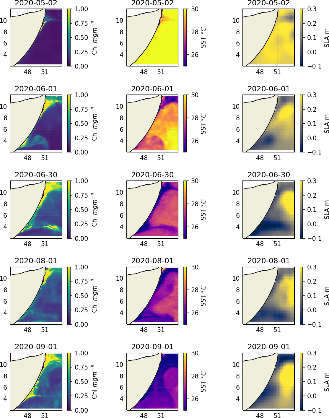
Figure 1 Example maps of the three different variables expected to be linked to upwelling over the SE monsoon season. Each row indicates a different day, over 2020, separated by 1 month. The variables are: (leftmost column) Chl, (centre column) SST, and (rightmost column) SLA.

2.2 Machine learning clustering approach

Initial visual analysis of Chl, SST, and SLA spatial distributions showed an overall good agreement between these variables over the SCU region (Figure 1), in line with theoretical expectations for upwelling waters (e.g., Letelier et al., 2009; Menna et al., 2016). During the upwelling season (May to September), an increased proportion of low SST, high Chl data is seen (Supplementary Figure 2) expected to be linked to upwelling. The change in the distribution of data indicate that clustering should be a suitable technique to delineate an upwelling surface signature within the data. A number of clustering approaches were explored in an initial testing phase, where the K-means learning algorithm was found to provide best results [i.e., more in line with expectations of a separate high Chl, low SST region – as identified by the scatter plots – when compared with other clustering approaches such as DBSCAN (Ester et al., 1996)]. This likely relates to the characteristics associated with the data, i.e., the data density and variability, in the Chl/SST variable space in this region.

K-means clustering allows a user selected number of clusters to be defined, i.e., the number of clusters is not a pre-defined automated process (Macqueen, 1967). As such a range of “K” values (i.e., number of clusters) were tested (see examples in Figures 2–4, and more details on the selection process in the Results below). Two different K-means based modelling approaches were assessed, a 2-variable (Chl and SST) and a 3-variable (Chl, SST, and SLA). Both K-means learning approaches were assessed visually and with clustering metrics (Calinski-Harabasz score shown here) to determine their suitability.

To fit the K-means based model, the data was subset, with only the reprocessed data between 2007 and 2020 used. First, only data from the Southwest Monsoon period were used, when the SCU is active (e.g., Schott, 1983), specifically only data from the months of May – September inclusive were used (Jebri et al., 2020). Once the temporal subsetting was done, fitting was based on a selection of 15% of the remaining data with 85% used for testing. The NRT data provided a further out of sample testing dataset. Data were first treated with outlier removal, whereby data exceeding the 99.5% quantile or lying below the 0.5% quantile were removed, before minmax scaling prior to fitting. The scaling and outlier removal reduce the sensitivity of clustering approaches to anomalies in the individual datasets used (Milligan and Cooper, 1988). This will also potentially reduce the volume of data required for accurate, reproducible fitting.

2.3 Extremes threshold classification approach

Once an upwelling surface signature has been identified, the upwelling indicators (e.g., Chl, SST, SLA) are classified to determine whether they represent an extreme event. This determination of extremes is made with a comparison against historical data in each grid cell (see e.g., Figure 1). All data from the historical period (2007-2020) in each individual grid cell were taken to define a historical distribution. This was done on a grid cell basis as, for example, some grid cells will always have high SST values, so would otherwise always be identified as extreme in SST (when compared to the distribution of the whole region). From this historical distribution, quantiles were used to determine thresholds for extreme classification. As this is classifying upwelling, only data identified as upwelling core (i.e., highest Chl, lowest SST – detailed fully in Section 3.1) in the clustering approach (detailed above) was considered. The classification of extreme events was determined from whether the grid cell value in a given image exceeded a minimum or maximum threshold (i.e., the peaks-over-threshold method – e.g., Lang et al., 1999). In such case, the event is classified as a high or low extreme in any or all of the upwelling indicators. The threshold value was determined using all historical data within a given grid cell using quantiles, a number of which were considered (5/95%, 15/85%, 25/75%) in lieu of an automated selection process (e.g., Lang et al., 1999).

Figure 5 shows an example of the methodology for the extremes classification approach, in this case for an extreme in SST, showing a scatter plot in Chl/SST space of data from within the upwelling core cluster. Alongside are two histograms, showing the distributions of SST (top right) and Chl (bottom left). The colours are indicative of the data being classified as an extreme low (blue) or high in SST (yellow), in this case marked as threshold quantiles of 15 and 85% of the data. A similar approach is applied to Chl data, although in that case a low extreme would be considered as non-upwelling and therefore is not indicated by the approach.

3 Results

3.1 Upwelling signature using the 2-variables (Chl - SST) K-means based model

K-means clustering relies on a predefined number of clusters “K” chosen by the user, that must be manually optimised (Macqueen, 1967). The elbow criterion is an approach to determining the optimal number of clusters. It works by calculating the metric Within Cluster Sum of Squares (WCSS) for a number of K values. The optimum number for “K” can then be determined by plotting K against WCSS and identifying the inflexion point (Thorndike, 1953). For the 2-variable (Chl and SST) model an optimum number of 4 regions is determined Figure 2. Scatter plots of a number of different K values are shown in Figure 3 with corresponding maps displayed in Figure 4. The smallest number of clusters (2) separates into a high Chl/low SST clustering region and a low Chl/high SST non-upwelling region (Figures 3, 4). Additional clusters, beyond these first two, add subdivision primarily in the mid-SST low-Chl space. Looking at maps of these different examples (Figure 4) these regions can be characterised as an upwelling core region (green), an upwelling surround or pre/post upwelling region (yellow), as well as two non-upwelling regions, divided primarily by their average temperature (blue and grey). A similar analysis is performed for a 3-variable model (Chl/SST/SLA) – see Supplementary Material.

FIGURE 2

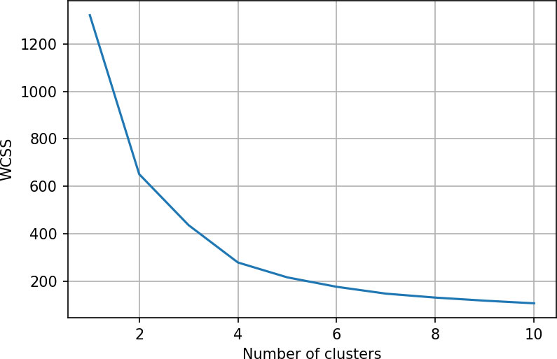
Figure 2 Elbow diagram indicating the performance for different pre-defined numbers of clusters. The inflexion point indicates the optimum number of clusters. This corresponds to the 2-variable model (Chl/SST).

FIGURE 3

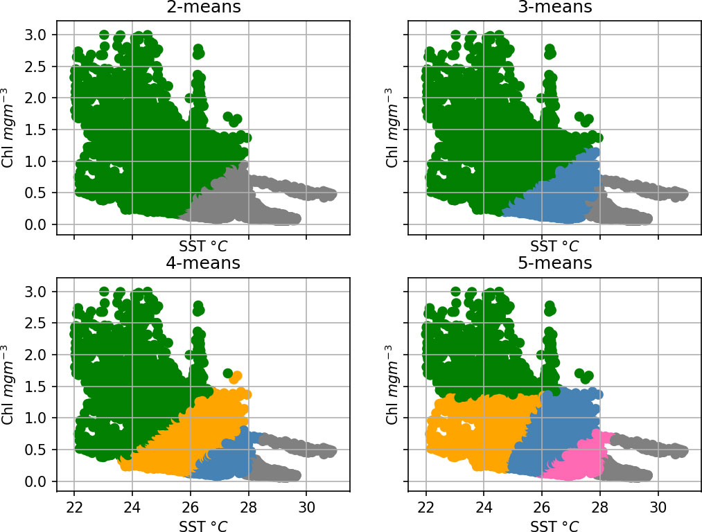
Figure 3 Scatter plots of SST against Chl with subplots representing different numbers of pre-defined clusters, and colours indicating the different clusters for the 2-variable model (Chl/SST).

FIGURE 4

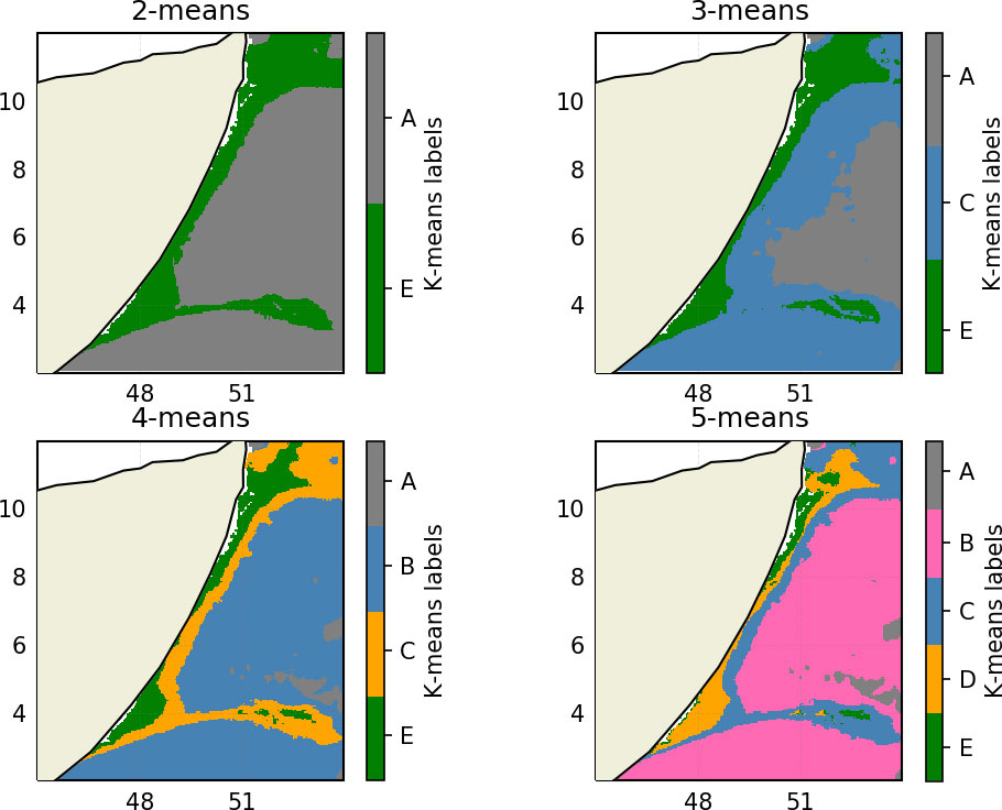
Figure 4 Maps showing the regions identified with clustering, using different numbers of pre-defined clusters corresponding to those shown in Figure 3. This corresponds to the 2-variable model (Chl/SST).

3.2 Performance comparison of 2-variable and 3-variable models

Once the clustering K-means based model (c.f. section 2.2) is fitted using a random sample (subset) of the reprocessed remote sensing data, it is then applied to the remaining subset and to the operational remote sensing data. An assessment of temporal performance (both interannual and seasonal respectively) of the two data types is shown in Figure 6 (blue and green lines) & Figure 7 (blue and green dots) using the metric Calinski-Harabasz Score, which represents the ratio between the dispersion within individual clusters to the dispersion between clusters, whereby a larger score indicates better clustering (Caliński and Harabasz, 1972). In terms of the historical reprocessed data, some small degree of interannual variability is seen, although seasonal variability is much stronger (Figure 6; blue and green lines). The seasonal clustering performance shows a peak in performance in July (Figure 7; blue and green dots). It should be noted that the portion of this variability that is related to clustering performance is unclear, with a considerable proportion instead likely relating to underlying variability of the data, for example the July peak in performance may relate to a stronger and more uniform upwelling signal. This is considered further in the discussion section.

FIGURE 5

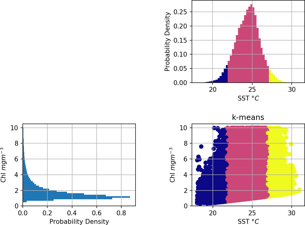
Figure 5 Example of extremes definition in SST space. (bottom right) Chl/SST scatter plot, (bottom left) Chl histogram, (top right) SST histogram. Dark blue indicates an extreme low in SST, yellow indicates an extreme high in SST.

FIGURE 6

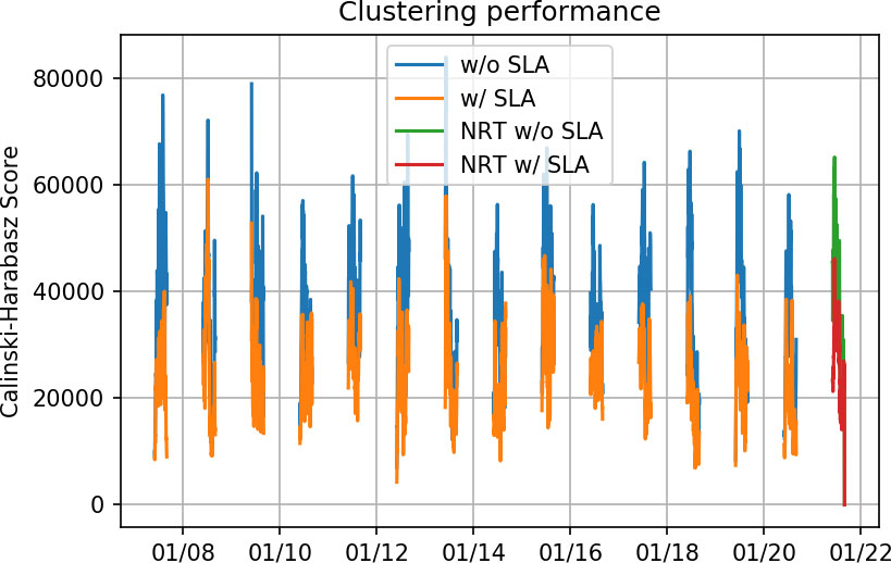
Figure 6 Clustering performance over the entire time series of the study, showing clustering models with and without the inclusion of SLA data, as well as the application to NRT data for both these cases.

FIGURE 7

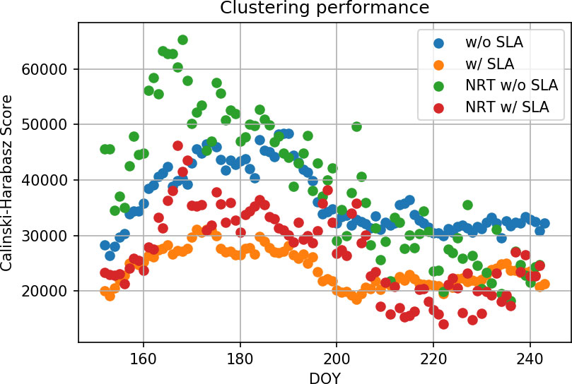
Figure 7 Average clustering performance over the seasonal cycle, showing clustering models with and without the inclusion of SLA data, as well as the application to NRT data for both these cases.

Like the 2-variable model, the 3-variable clustering model is fitted using a random sample (subset) of the reprocessed remote sensing data before application to the operational remote sensing data. An assessment of temporal performance (both interannual and seasonal respectively) of the two data types is shown in Figure 6 (orange and red lines) & Figure 7 (orange and red dots), showing similar temporal variability to the 2-variable model. However, in all cases the 3-variable model shows worse performance. Due to the slightly worse performance of the 3-variable model (i.e., that also including SLA), we decided to continue with the 2-variable model (i.e., Chl and SST only) for the analysis of extreme upwelling events. More details behind this decision can be found in the discussion.

3.3 “Upwelling Watch”: upwelling NRT extreme events using the threshold classification

The maps in Figure 9 show the results from the application of the extremes threshold classification approach to one day of NRT data in 2021, alongside the underlying maps showing the SST and Chl data, as well as the clustering identification results. As detailed in the methodology, only the upwelling core cluster is used when identifying upwelling extremes. In this case there is shown to be one large area of high extreme in Chl that spans much of the South of the upwelling core cluster. The SST data shows areas of both high and low extremes. There is a small area of high extremes in the East and two areas of low extremes, in the North and in the South of the upwelling region; the South shows a partial overlap with the high extremes in Chl.

4 Discussion

In this study, two K-means based clustering approaches for upwelling detection were used, leading to slightly different clustering performance. One K-means clustering model was fitted also using information for SLA (i.e., Chl/SST/SLA), the other was fitted without this information (i.e., Chl/SST only). A spatial comparison of both clustering models is included in Figure 8, using an example from one day of NRT data, also showing the underlying variables used by the clustering technique. A reasonable correlation in the spatial patterns of the three variables over the upwelling region is seen, however the inclusion of SLA in the K-means model leads to slightly worse performance. This could relate to two factors; the SLA model picks up more features that do not directly relate to the targeted coastal upwelling (e.g., SC associated gyres) and secondly the coarser spatial resolution (25 km vs 4-5 km for the other two variables). This leads to, when a region boundary is more dominantly SLA defined, spatial boundaries that are not smooth and instead take the coarser resolution of the SLA product as well as the omission of smaller scale features. It may be possible in future that an improved resolution SLA product (e.g., from the upcoming SWOT mission) could be a useful addition to this upwelling identification system; alternatively, SLA data from models could be another possible source of this information.

FIGURE 8

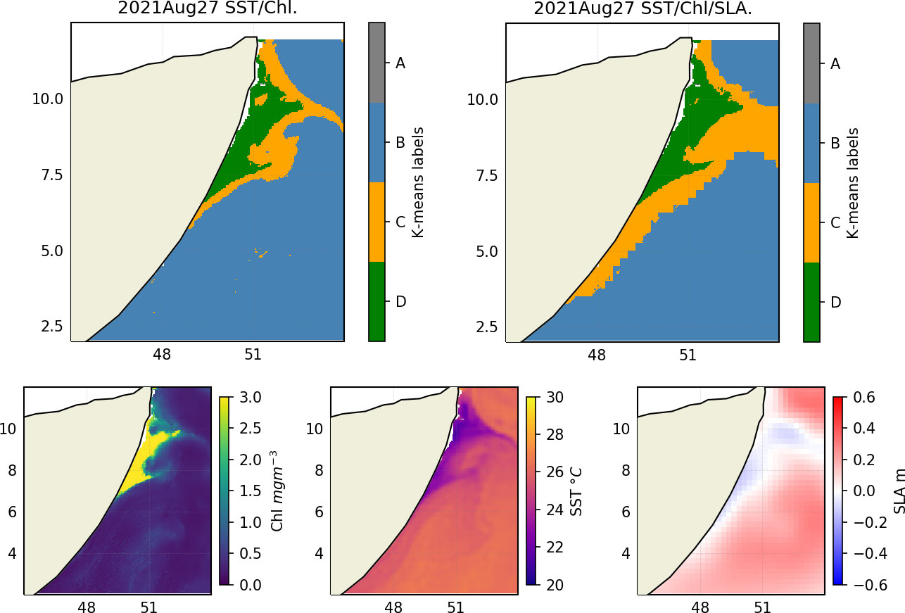
Figure 8 Example of image showing one day of the two clustering models. (Top left) clustering using Chl and SST only, (top right) clustering using Chl, SST, and SLA. The bottom row shows the three underlying variables: Chl (bottom left), SST (bottom centre), and SLA (bottom right).

Three parameters associated with upwelling (Chl, SST, and SLA) were directly explored in this manuscript. Current and wind vectors were also explored in a preliminary analysis although they were not found to have a strong correlation with the Chl and SST variables. Other variables have also been shown to impact Chl productivity in upwelling regions. For example, precipitation has been shown to have an indirect impact on Chl productivity through influence on nutrient input via riverine discharge into coastal regions (e.g., Shafeeque et al., 2019). Precipitation data was not incorporated into our methodology as precipitation primarily affects the coastal region (the majority of our study region is open ocean) and is currently of limited spatial resolution (e.g., 1° for the Global Precipitation Climatology Product, Huffman et al., 2001). Aerosols and dust have also been shown to have some very limited impact on chl productivity in the Somali offshore region (Shafeeque et al., 2017), and so they are not incorporated into our methodology.

There are a small number of limitations that affect the remote sensing data used here, although they should have limited impact. Remotely sensed Chl-a cannot be retrieved when there is cloud cover, as clouds block visible light, this is partially compensated by the use of an L4 dataset. The L4 GlobColour dataset fills missing data (due to cloud coverage) by using the most recently available value in a grid cell. SST data is similarly affected by cloud cover, at infrared wavelengths, although this is similarly compensated by use of an L4 dataset that incorporates data from microwave sensors. Additionally, Chl-a values are typically overestimated near the coast due to the impact of atmospheric aerosols and dust as well as additional constituents in the water column, including Coloured Dissolved Organic Matter (CDOM) (Schollaert et al., 2003; Hyde et al., 2007; Mélin et al., 2007). Regional studies have shown that radiometric biases can exceed ±5% for data within 25km of the coast (Bulgarelli et al., 2017). SLA data is also known to be impacted near the coast, where altimeters can be contaminated by land falling within the footprint of the altimetry instruments as well by the impact of tides and other high frequency events; data within 15km of the coast are generally considered inaccurate (The Climate Change Initiative Coastal Sea Level Team, 2020). These limitations close to the coast are largely mitigated by the study area primarily being open ocean and by the use of outlier removal.

The application of the K-means model fitted using historical reprocessed data to operational data performs well and is within the bounds produced by the historical reprocessed data (both seasonally and interannually, Figures 6, 7). This indicates the model fit is likely to continue to be applicable to incoming reprocessed data for the foreseeable future, provided there are no major changes in the primary Chl/SST relationships in this region. It is also feasible that this method could be adapted in future to detect such changes. However, assessing the overall performance of these K-means based models can be somewhat challenging in two ways. First, although there is good theoretical understanding of upwelling drivers and relevant biogeochemical response, in situ data, which compared to satellite data have the advantage of sampling the ocean subsurface, are rarely available in this region. Conversely, while ocean model data is available at depth, models are currently poor at describing vertical (upwelling) velocities, so there is a dependency on secondary parameters (e.g., nutrient and Chl concentrations indicative of the biological response). These secondary parameters can have a spatial coverage different from the actual upwelling site. Comparison in future with fishing data may allow some assessment of the performance, assuming a higher abundance of fish in these productive upwelling regions, although the limited spatial resolution of available fishing datasets (e.g., up to 0.5°; Pauly et al., 2020) would make this challenging at present. The second factor challenging performance assessment is the use of traditional clustering metrics (e.g., Calinski-Harabasz score here); as the data itself changes temporally, the metrics will also reflect this variability rather than solely clustering performance (e.g., Wu et al., 2009). The data considered in each “scene” (i.e., one day of data) differs between days. This will happen on a day-to-day basis, seasonally, and also interannually, as the variables change in response to drivers beyond simply upwelling. This will in turn lead to “apparent” changes in clustering performance, in traditional clustering metrics (e.g., the Calinski-Harabasz score), that do not necessarily reflect any change in true performance. New metrics, or normalisation of existing metrics, that are robust to this may help improve assessment of such clustering approaches in future (e.g., Wu et al., 2009).

In a potential “Upwelling Watch” service, being able to not only identify upwelling but also classify extreme events will be of great use to potential end users. For the example found in Figure 9 part of the upwelling region is identified as a high extreme in Chl and low extreme in SST. In order to classify upwelling events as extremes, a number of thresholds were explored, in this case based on quantiles at 5-15% and 75-95% of the data (Figure 7). Each of these thresholds thus corresponds to a different proportion of data classified as being extreme. However, the optimum proportion has not been identified in this study. Instead, it may vary depending on the subject of interest, for example for potential fisheries end users it may depend on the type of fish being targeted, noting that there can be lags between Chl productivity and fish abundance (Menon et al., 2019; Kizenga et al., 2021). As such in a potential “Upwelling Watch” service, the thresholds for this may be a user selectable option. Alternatively, to allow a more informed comparison and selection of these threshold options, future work on comparing these thresholds with fishing data may help identify the ideal thresholds.

FIGURE 9

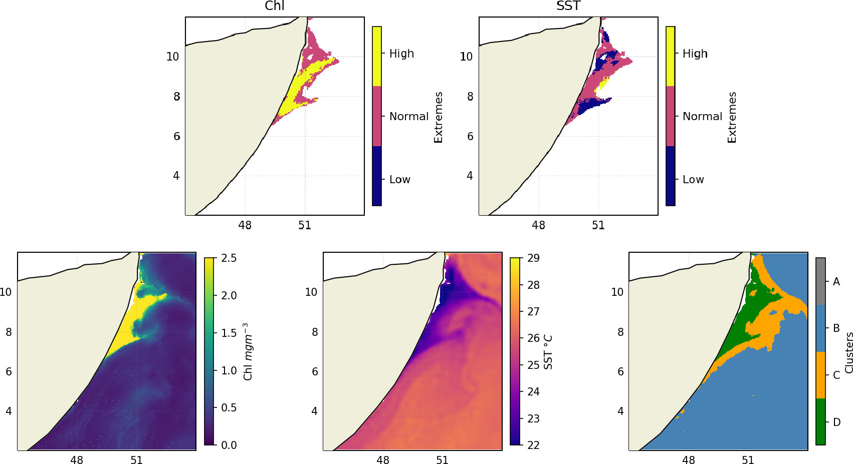
Figure 9 Example of extremes classification for (top left) Chl, (top right) SST, alongside the underlying variables: Chl (bottom left), SST (bottom centre), and upwelling classification (bottom right).

The clustering method is based on identification of regions within Chl/SST space. As such, other ocean features such as mesoscale eddies and oceanic fronts may have a similar signature to upwelling. Evidence of the detection of an eddy can be seen in Supplementary Video 1 between the 17^th and 21^st of August, classified by the method as part of the upwelling surround or pre/post upwelling region. The analysis of fronts in this region is the focus of ongoing work although the main thermal fronts in this region have been shown to correspond with the typical Somali upwelling signature (e.g., Wang et al., 2021). When applying this method, care should be taken to avoid contamination of the signal by eddies and fronts; if it is necessary to separate these features in future work, joint application of automated eddy and front detection techniques (e.g., Belkin, 2021; Mauzole, 2022) alongside the upwelling detection could be performed.

The clustering K-means model is currently fitted, and geophysical variables selected for, the SCU. This method can be expanded in future, either to the rest of the WIO or indeed additional seasonal upwelling systems globally, but with some adaptations. It is possible that some covariates other than Chl and SST become more important for successful clustering. This may be particularly relevant in, for example, regions where there is substantial riverine input, which is typically higher Chl at high SST, rather than the high Chl/low SST expected as an upwelling signature. Another example would be areas where primary production is not limited by nutrient availability (e.g., at higher latitudes); the addition of nutrients via upwelling in these areas may lead to a more muted response in Chl. Although potential extra remotely sensed covariates will still be limited by the available resolution, as in the case of SLA, model information may possibly be used to supplement remote sensing data.

5 Conclusions and perspectives

An unsupervised ML clustering (K-means based) approach was used to detect and then classify seasonal upwelling surface signature off the Somali coast using satellite observations. This approach successfully delineates upwelling core and surrounds as well as non-upwelling ocean regions. The technique is shown to be temporally robust (seasonally and interannually) with accurate classification of NRT data not used in the fitting of the classification model. Once upwelling regions have been identified, classification of extreme upwelling events was performed using a threshold approach that includes confidence intervals derived from historical data. These approaches, that we call “Upwelling Watch”, are designed to be adaptable to meet users’ needs.

Due to the high productivity in seasonal coastal upwelling systems, such as analysed here in the WIO, they support a large volume of fishing activity sustaining food security in the region for millions of people (Taylor et al., 2019). At the same time, upwelling systems can be areas of reduced oxygen and more pronounce acidification (e.g., Kämpf and Chapman, 2016), negatively impacting marine ecosystems. Thus, extremes in upwelling along with general upwelling variability can directly affect fishing catch success rates and the health of marine ecosystems in general. This “Upwelling Watch” service, designed to detect these upwelling systems and their anomalous behaviour, can be very useful provided it is accompanied by schemes to raise awareness and maximise use rates for those most in need of it. Furthermore, local fisheries data collection and analysis needs to work hand-in-hand with this service to be able to identify and document biological consequences of the extreme upwelling events. An implementation scheme alongside the full development of the system could involve interactions with local management, governments, and NGOs in order to aid in communication of its benefits.

This work has shown promise within the SCU system with aims to expand it in future to the rest of the WIO using similar clustering techniques although recognising that different upwelling systems can provide their own unique problems, potentially requiring adaptations to both the method and geophysical information used. This “Upwelling Watch” method can aid fisheries management, by potential defining target areas for fishing. The “Upwelling Watch” method may also provide broader scientific value by providing a definition of upwelling regions, and classification of their modes of variability. This subset of data can then be further analysed in numerous ways. Examples might include studying temporal and spatial dynamics of upwelling, addressing potential questions such as whether upwelling is changing in its spatial extent as well as quantifying marine heatwaves and cold spells and associated extremes of Chl (green waves), in this and potentially other seasonal upwelling regions.

Data availability statement

Publicly available datasets were analyzed in this study. This data can be found here: https://resources.marine.copernicus.eu/product-detail/OCEANCOLOUR_GLO_CHL_L4_NRT_OBSERVATIONS_009_033/INFORMATION https://resources.marine.copernicus.eu/product-detail/OCEANCOLOUR_GLO_CHL_L4_REP_OBSERVATIONS_009_082/INFORMATION https://resources.marine.copernicus.eu/product-detail/SST_GLO_SST_L4_NRT_OBSERVATIONS_010_001/INFORMATION https://resources.marine.copernicus.eu/product-detail/SEALEVEL_GLO_PHY_CLIMATE_L4_MY_008_057/INFORMATION https://resources.marine.copernicus.eu/product-detail/SEALEVEL_GLO_PHY_L4_NRT_OBSERVATIONS_008_046/INFORMATION

Author contributions

Methodology and investigations: MH. Writing—original draft preparation: MH. Writing—review and editing: all. Supervision: FJ, MS, EP. Project administration: EP. All authors contributed to the article and approved the submitted version.

Funding

This study was supported by the Global Challenges Research Fund (GCRF) under NERC grant NE/P021050/1 in the framework of the SOLSTICE-WIO project (https://www.solstice-wio.org/) as well as the UK National Capability project FOCUS (NE/X006271/1).

Acknowledgments

All data used in this study was sourced from the Copernicus Marine Service (CMEMS- marine.copernicus.eu). SST data was produced by the OSTIA project, Chl data by the Copernicus-GlobColour team, and SLA was processed by CMEMS. The authors would like to thank those involved for producing these datasets and for making them freely available.

Conflict of interest

The authors declare that the research was conducted in the absence of any commercial or financial relationships that could be construed as a potential conflict of interest.

Publisher’s note

All claims expressed in this article are solely those of the authors and do not necessarily represent those of their affiliated organizations, or those of the publisher, the editors and the reviewers. Any product that may be evaluated in this article, or claim that may be made by its manufacturer, is not guaranteed or endorsed by the publisher.

Supplementary material

The Supplementary Material for this article can be found online at: https://www.frontiersin.org/articles/10.3389/fmars.2022.950733/full#supplementary-material

References

Ardyna M., Claustre H., Sallée J.-B., D'Ovidio F., Gentili B., van Dijken G., et al. (2017). Delineating environmental control of phytoplankton biomass and phenology in the Southern Ocean. Geophys. Res. Lett. 44 (10), 5016–5024. doi: 10.1002/2016GL072428

CrossRef Full Text | Google Scholar

Baars M. A., Schalk P. H., Veldhuis J. W. (1998). “Seasonal fluctuations in plankton biomass and productivity in the ecosystems of the Somali current, gulf of Aden, and southern red sea,”, in Large Marine ecosystems of the Indian ocean: Assessment, sustainability, and management (Oxford: Blackwell Science), 143–174.

Google Scholar

Bakun A., Roy C., Lluch-Cota S. (1998). Coastal upwelling and other processes regulating ecosystem productivity and fish production in the Western Indian ocean. Large Mar. Ecosyst. Indian Ocean Assessment Sustain. Manage 103–139.

Google Scholar

Barber R. T. (2001). Upwelling ecosystems. Encycl. Ocean Sci. 6, 3128–3135. doi: 10.1006/rwos.2001.0295

CrossRef Full Text | Google Scholar

Beal L. M., Donohue K. A. (2013). The great whirl: Observations of its seasonal development and interannual variability. J. Geophys. Res. Ocean. 118, 1–13. doi: 10.1029/2012JC008198

CrossRef Full Text | Google Scholar

Belkin I. M. (2021). Review remote sensing of ocean fronts in marine ecology and fisheries. Remote Sens. 13, 1–22. doi: 10.3390/rs13050883

CrossRef Full Text | Google Scholar

Bengio Y., Courville A., Vincent P. (2013). Representation learning: A review and new perspectives. IEEE Trans. Pattern Anal. Mach. Intell. 35, 1798–1828. doi: 10.1109/TPAMI.2013.50

PubMed Abstract | CrossRef Full Text | Google Scholar

Bulgarelli B., Kiselev V., Zibordi G. (2017). Adjacency effects in satellite radiometric products from coastal waters: a theoretical analysis for the northern Adriatic Sea. Appl. Opt. 56, 854. doi: 10.1364/ao.56.000854

PubMed Abstract | CrossRef Full Text | Google Scholar

Caliński T., Harabasz J. (1972). A dendrite method for cluster analysis. Commun. Stat. 3, 1–27. doi: 10.1080/03610927408827101

CrossRef Full Text | Google Scholar

Chatterjee A., Kumar B. P., Prakash S., Singh P. (2019). Annihilation of the Somali upwelling system during summer monsoon. Sci. Rep. 9, 1–14. doi: 10.1038/s41598-019-44099-1

PubMed Abstract | CrossRef Full Text | Google Scholar

Chen Y., Jiang H., Li C., Jia X., Ghamisi P (2016). “Deep feature extraction and classification of hyperspectral images based on convolutional neural networks,” in IEEE Transactions on Geoscience and Remote Sensing. 6232–6251.

Google Scholar

Cheng E. J., Chou K. P., Rajora S., Jin B. H., Tanveer M., Lin C. T., et al. (2019). Deep sparse representation classifier for facial recognition and detection system. Pattern Recognit. Lett. 125, 71–77. doi: 10.1016/j.patrec.2019.03.006

CrossRef Full Text | Google Scholar

Cushing D. H. (1971). Upwelling and the production of fish. Adv. Mar. Biol. 9, 255–300. doi: 10.1016/S0065-2881(08)60344-2

CrossRef Full Text | Google Scholar

DeCastro M., Sousa M. C., Santos F., Dias J. M., Gómez-Gesteira M. (2016). How will Somali coastal upwelling evolve under future warming scenarios? Sci. Rep. 6, 1–9. doi: 10.1038/srep30137

PubMed Abstract | CrossRef Full Text | Google Scholar

Devred E., Sathyendranath S., Platt T. (2007). Delineation of ecological provinces using ocean colour radiometry. Mar. Ecol. Prog. Ser. 346, 1–13. doi: 10.3354/meps07149

CrossRef Full Text | Google Scholar

Donlon C. J., Martin M., Stark J., Roberts-Jones J., Fiedler E., Wimmer W. (2012). The operational Sea surface temperature and Sea ice analysis (OSTIA) system. Remote Sens. Environ. 116, 140–158. doi: 10.1016/j.rse.2010.10.017

CrossRef Full Text | Google Scholar

Ester M., Kriegel H., Xu X., Miinchen D. (1996). A density-based algorithm for discovering clusters in Large spatial databases with noise. Proc. Second Int. Conf. Knowl. Discov. Data Min. 1, 226–231. doi: 10.5555/3001460.3001507

CrossRef Full Text | Google Scholar

Findlater J. (1971). Mean monthly airflow at low levels over the western Indian ocean. Geophys. Mem. XVI, 115.

Google Scholar

Garnesson P., Mangin A., D’Andon O. F., Demaria J., Bretagnon M. (2019). The CMEMS GlobColour chlorophyll a product based on satellite observation: Multi-sensor merging and flagging strategies. Ocean Sci. 15, 819–830. doi: 10.5194/os-15-819-2019

CrossRef Full Text | Google Scholar

Huffman G. J., Adler R. F., Morrissey M. M., Bolvin D. T., Curtiss S., Joyce R., et al. (2001). Global precipitation at one-degree daily resolution from multisatellite observations. J. Hydrometeorol. 2, 36–50.

Google Scholar

Hyde K. J. W., O’Reilly J. E., Oviatt C. A. (2007). Validation of SeaWiFS chlorophyll a in Massachusetts bay. Cont. Shelf Res. 27, 1677–1691. doi: 10.1016/j.csr.2007.02.002

CrossRef Full Text | Google Scholar

Jacobs Z. L., Jebri F., Raitsos D. E., Popova E., Srokosz M., Painter S. C., et al. (2020a). Shelf-break upwelling and productivity over the north Kenya banks: The importance of Large-scale ocean dynamics. J. Geophys. Res. Ocean. 125, 1–18. doi: 10.1029/2019JC015519

CrossRef Full Text | Google Scholar

Jacobs Z. L., Jebri F., Srokosz M., Raitsos D. E., Painter S. C., Nencioli F., et al. (2020b). A major ecosystem shift in coastal east African waters during the 1997/98 super El niño as detected using remote sensing data. Remote Sens. 12, 3127. doi: 10.3390/RS12193127

CrossRef Full Text | Google Scholar

Jebri F., Jacobs Z. L., Raitsos D. E., Srokosz M., Painter S. C., Kelly S., et al. (2020). Interannual monsoon wind variability as a key driver of East African small pelagic fisheries. Sci. Rep. 10, 1–15. doi: 10.1038/s41598-020-70275-9

PubMed Abstract | CrossRef Full Text | Google Scholar

Jebri F., Raitsos D. E., Gittings J. A., Jacobs Z. L., Srokosz M., Gornall J., et al. (2022a). Unravelling links between squid catch variations and biophysical mechanisms in south African waters. Deep. Res. Part II Top. Stud. Oceanogr. 196, 105028. doi: 10.1016/j.dsr2.2022.105028

CrossRef Full Text | Google Scholar

Jebri F., Srokosz M., Jacobs Z. L., Nencioli F., Popova E. (2022b). Earth observation and machine learning reveal the dynamics of productive upwelling regimes on the agulhas bank. Front. Mar. Sci. 9. doi: 10.3389/fmars.2022.872515

PubMed Abstract | CrossRef Full Text | Google Scholar

Jouini M., Béranger K., Arsouze T., Beuvier J., Thiria S., Crépon M., et al. (2016). The Sicily channel surface circulation revisited using a neural clustering analysis of a high-resolution simulation. J. Geophys. Res. Ocean. 121, 4545–4567. doi: 10.1002/2015JC011472

CrossRef Full Text | Google Scholar

Kämpf J., Chapman P. (2016). Upwelling systems of the world: A scientific journey to the most productive marine ecosystems (Switzerland: Springer International Publishing). doi: 10.1007/978-3-319-42524-5

CrossRef Full Text | Google Scholar

Kizenga H. J., Jebri F., Shaghude Y., Raitsos D. E., Srokosz M., Jacobs Z. L., et al. (2021). Variability of mackerel fish catch and remotely-sensed biophysical controls in the eastern pemba channel. Ocean Coast. Manage. 207, 105593. doi: 10.1016/j.ocecoaman.2021.105593

CrossRef Full Text | Google Scholar

Lakshmi R. S., Chatterjee A., Prakash S., Mathew T. (2020). Biophysical interactions in driving the summer monsoon chlorophyll bloom off the Somalia coast. J. Geophys. Res. Ocean. 125. doi: 10.1029/2019JC015549

CrossRef Full Text | Google Scholar

Lang M., Ouarda T. B. M. J., Bobée B. (1999). Towards operational guidelines for over-threshold modeling. J. Hydrol. 225, 103–117. doi: 10.1016/S0022-1694(99)00167-5

CrossRef Full Text | Google Scholar

Letelier J., Pizarro O., Nun S. (2009). Seasonal variability of coastal upwelling and the upwelling front off central Chile. J. Geophys. Res. 114, 1–16. doi: 10.1029/2008JC005171

CrossRef Full Text | Google Scholar

Liu Y., Weisberg R. H. (2005). Patterns of ocean current variability on the West Florida shelf using the self-organizing map. J. Geophys. Res. Ocean. 110, 1–12. doi: 10.1029/2004JC002786

CrossRef Full Text | Google Scholar

Macqueen J. (1967). “Some methods for classification and analysis of multivariate observations,” in 5th Berkeley symposium on mathematical statistics and probability, 281–297.

Google Scholar

Mauzole Y. L. (2022). Objective delineation of persistent SST fronts based on global satellite observations. Remote Sens. Environ. 269, 112798. doi: 10.1016/j.rse.2021.112798

CrossRef Full Text | Google Scholar

Mccreary J. P., Kohler K. E., Hood R. R., Olson D. B. (1996). A four-component ecosystem model of biological activity in the Arabian Sea. Prog. Oceanogr. 37, 193–240. doi: 10.1016/S0079-6611(96)00005-5

CrossRef Full Text | Google Scholar

Mélin F., Zibordi G., Berthon J. F. (2007). Assessment of satellite ocean color products at a coastal site. Remote Sens. Environ. 110, 192–215. doi: 10.1016/j.rse.2007.02.026

CrossRef Full Text | Google Scholar

Menna M., Faye S., Poulain P., Centurioni L., Lazar A., Gaye A., et al. (2016). Upwelling features off the coast of north-western Africa in 2009-2013. Boll. di Geofis. Teor. ed Appl. 57, 71–86. doi: 10.4430/bgta0164

CrossRef Full Text | Google Scholar

Menon N. N., Sankar S., Smitha A., George G., Shalin S. (2019). Satellite chlorophyll concentration as an aid to understanding the dynamics of Indian oil sardine in the southeastern Arabian Sea. Mar. Ecol. Prog. Ser. 617-618, 137–147. doi: 10.3354/meps12806

CrossRef Full Text | Google Scholar

Milligan G. W., Cooper M. C. (1988). A study of standardization of variables in cluster analysis. J. Classif. 5, 181–204. doi: 10.1007/BF01897163

CrossRef Full Text | Google Scholar

Pastore V. P., Zimmerman T. G., Biswas S. K., Bianco S. (2020). Annotation-free learning of plankton for classification and anomaly detection. Sci. Rep. 10, 1–15. doi: 10.1038/s41598-020-68662-3

PubMed Abstract | CrossRef Full Text | Google Scholar

Pauly D., Zeller D., Palomares M. L. D. (Eds.) (2020). “Sea Around us concepts,” in Design and data (seaaroundus.org). Available at: https://www.seaaroundus.org/citation-policy/.

Google Scholar

Reygondeau G., Longhurst A., Martinez E., Beaugrand G., Antoine D., Maury O. (2013). Dynamic biogeochemical provinces in the global ocean. Global Biogeochem. Cycles 27, 1046–1058. doi: 10.1002/gbc.20089

CrossRef Full Text | Google Scholar

Richardson A. J., Risi En C., Shillington F. A. (2003). Using self-organizing maps to identify patterns in satellite imagery. Prog. Oceanogr. 59, 223–239. doi: 10.1016/j.pocean.2003.07.006

CrossRef Full Text | Google Scholar

Schollaert S. E., Yoder J. A., O’Reilly J. E., Westphal D. L. (2003). Influence of dust and sulfate aerosols on ocean color spectra and chlorophyll a concentrations derived from SeaWiFS off the U.S. East Coast. J. Geophys. Res. Ocean. 108, 3191. doi: 10.1029/2000jc000555

CrossRef Full Text | Google Scholar

Schott F. (1983). Monsoon response of the Somali Current and associated upwelling. Prog. Oceanogr. 12, 357–381. doi: 10.1016/0079-6611(83)90014-9

CrossRef Full Text | Google Scholar

Schott F. A., McCreary J. P. (2001). The monsoon circulation of the Indian ocean. Prog. Oceanogr. 51, 1–123. doi: 10.1016/S0079-6611(01)00083-0

CrossRef Full Text | Google Scholar

Schott F. A., Xie S. P., McCreary J. P. (2009). Indian Ocean circulation and climate variability. Rev. Geophys. 47, 1–46. doi: 10.1029/2007RG000245

CrossRef Full Text | Google Scholar

Shafeeque M., Sathyendranath S., George G. (2017). Comparison of seasonal cycles of phytoplankton chlorophyll, aerosols, winds and Sea-surface temperature off Somalia. Front. Mar. Sci. 4, 386. doi: 10.3389/fmars.2017.00386

CrossRef Full Text | Google Scholar

Shafeeque M., Shah P., Platt T., Sathyendranath S., Menon N. N. (2019). Effect of precipitation on chlorophyll-a in an upwelling dominated region along the West coast of India. J. Coast. Res. doi: 10.2112/SI86-032.1

CrossRef Full Text | Google Scholar

Shi W., Morrison J. M., Böhm E., Manghnani V. (2000). The Oman upwelling zone during 1993, 1994 and 1995. Deep. Res. Part II Top. Stud. Oceanogr. 47, 1227–1247. doi: 10.1016/S0967-0645(99)00142-3

CrossRef Full Text | Google Scholar

Strub P. T., James C., Combes V., Matano R. P., Piola A. R., Palma E. D., et al. (2015). Altimeter-derived seasonal circulation on the southwest Atlantic shelf: 27°–43°S. J. Geophys. Res. Ocean. 120 (5), 3391–3418. doi: 10.1002/2015JC010769

CrossRef Full Text | Google Scholar

Taylor S. F. W., Roberts M. J., Milligan B., Ncwadi R. (2019). Measurement and implications of marine food security in the Western Indian ocean: an impending crisis? Food Secur. 11, 1395–1415. doi: 10.1007/s12571-019-00971-6

CrossRef Full Text | Google Scholar

The Climate Change Initiative Coastal Sea Level Team. (2020). Coastal sea level anomalies and associated trends from Jason satellite altimetry over 2002-2018. Sci. Data 7, 357. doi: 10.1038/s41597-020-00694-w

PubMed Abstract | CrossRef Full Text | Google Scholar

Thorndike R. L. (1953). Who belongs in the family? Psychometrika 18, 267–276. doi: 10.1007/BF02289263

CrossRef Full Text | Google Scholar

Varela R., Álvarez I., Santos F., DeCastro M., Gómez-Gesteira M. (2015). Has upwelling strengthened along worldwide coasts over 1982-2010? Sci. Rep. 5, 1–15. doi: 10.1038/srep10016

CrossRef Full Text | Google Scholar

Wang Y., Ma W., Zhou F., Chai F. (2021). Frontal variability and its impact on chlorophyll in the Arabian Sea. J. Mar. Syst. 218, 103545. doi: 10.1016/j.jmarsys.2021.103545

CrossRef Full Text | Google Scholar

Wiggert J. D., Hood R. R., Banse K., Kindle J. C. (2005). Monsoon-driven biogeochemical processes in the Arabian Sea. Prog. Oceanogr. 65, 176–213. doi: 10.1016/j.pocean.2005.03.008

CrossRef Full Text | Google Scholar

Wu J., Xiong H., Chen J. (2009). Proceedings of the 25th ACM SIGKDD International Conference on Knowledge Discovery & Data Mining. (New York: Association for Computing Machinery).

Google Scholar

Zhang C., Sargent I., Pan X., Li H., Gardiner A., Hare J., et al. (2018). An object-based convolutional neural network (OCNN) for urban land use classification. Remote Sens. Environ. 216, 57–70. doi: 10.1016/j.rse.2018.06.034

CrossRef Full Text | Google Scholar

Zheng H., Wang R., Yu Z., Wang N., Gu Z., Zheng B. (2017). Automatic plankton image classification combining multiple view features via multiple kernel learning. BMC Bioinf. 18, 1–18. doi: 10.1186/s12859-017-1954-8

CrossRef Full Text | Google Scholar