Assessing the viability of estimating baleen whale abundance from tourist vessels

Introduction

Baleen whales are an important consumer in polar regions, migrating from winter breeding grounds in low latitudes to high latitudes to acquire most of their annual energy budget (Horton et al., 2022). Most populations of baleen whales are recovering from industrialized whaling during the mid-part of the 20^th century (Baker and Clapham, 2004; Leaper and Miller, 2011; Tulloch et al., 2019) and are again dominating polar food webs (Ratnarajah et al., 2014; Ratnarajah et al., 2016; Savoca et al., 2021). However, we have a limited understanding of current population trends for many baleen whale species, particularly those which do not winter and/or migrate coastally, e.g., blue (Balaenoptera musculus), fin (Balaenoptera physalus), Antarctic minke (Balaenoptera bonaerensis, herein, minke) and sei (Balaenoptera borealis) whales for the southern hemisphere, for which the Southern Ocean foraging grounds may represent a single geographic location where the entire population can be surveyed simultaneously.

This study focuses on the southwest Atlantic sector of the Southern Ocean which is a hotspot for human and biological activity in the Southern Ocean (Tin et al., 2009; Tin et al., 2014; Bender et al., 2016; Erbe et al., 2019; Palmowski, 2020). It is also one of the fastest-warming regions in the Southern Ocean experiencing significant changes to sea-ice conditions (Carrasco et al., 2021; Lin et al., 2021) and the focus of the majority of the current krill fishing effort (Kawaguchi and Nicol, 2020). The current trigger limit for the catch of Antarctic krill (Euphausia superba) is based on a precautionary fishery approach managed by the Convention for the Conservation of Marine and Antarctic Living Resources (CCAMLR), to avoid potentially negative effects on krill populations and krill-dependent predators. The status of the recovering baleen whale populations foraging in the southwest Atlantic sector is unclear (Erbe et al., 2019). This is despite baleen whales being potentially the greatest consumers of Antarctic krill in the Southern Ocean (Baines et al., 2021; Warwick-Evans et al., 2021) and that the competitive relationships between baleen whales and other krill predators are likely to be as influential on the demographic signals monitored for krill fishing management as climate change and krill fishing itself (Ainley et al., 2006; Trivelpiece et al., 2011; McMahon et al., 2019). Annual monitoring of baleen whale abundance on foraging grounds, from which to estimate aggregate krill consumption by krill predators, will enhance CCAMLR’s Ecosystem-based Management (EBM) of the krill fishery.

While there is a need for surveys of baleen whale populations on Southern Ocean foraging grounds, ship-based surveys have been restricted spatially (e.g., Santora et al., 2014; Johannessen et al., 2022), temporally (e.g., Headly et al., 2001; Baines et al., 2021), or spatiotemporally (e.g., Herr et al., 2016; Herr et al., 2019; Bassoi et al., 2020). As illustrated by the 19-year gap between broad-scale surveys of the southwest Atlantic sector of the Southern Ocean by CCAMLR (Hedley et al., 2001; Baines et al., 2021) and the cessation of International Whaling Commission (IWC), IDCR/SOWER circumpolar surveys in the early 2000s (Branch and Butterworth, 2001a; Branch and Butterworth, 2001b). Determining ocean basin-scale abundance of baleen whales foraging in the Southern Ocean and inferring environmental, and/or prey-mediated drivers of baleen whale densities in both time and space has therefore proved elusive (El-Gabbas et al., 2020).

Increased collaborations between the tourist industry and scientific endeavors in recent years (e.g., the polar collective) have provided the opportunity to better estimate baleen whale abundance (Johannessen et al., 2022). Before the COVID-19 pandemic, Antarctic tourism was undergoing year-on-year growth (Lynch et al., 2010; Bender et al., 2016; Palmowski, 2020), a trend that after the pandemic-driven hiatus is expected to continue (IAATO Report, 2020). Antarctic tourist ships thus represent platforms of opportunity for repeated and ongoing surveys of baleen whales in the Southern Ocean, though several challenges exist.

Ship-based line transect distance sampling is the common method for surveying air-breathing predators at sea (Buckland et al., 2001; Thomas et al., 2010). For baleen whales, this method involves a vessel passing through a study area, typically along an a priori-designed survey track with trained observers logging animal sightings and recording their perpendicular distance to the transect line during defined periods of effort. Detection functions describe the relationship between the number of sightings and their perpendicular distance to the transect line, which generally decreases as the perpendicular distance from the transect line increases (Thomas et al., 2010). The ability to detect animals along a transect is influenced by several factors in addition to distance, such as sighting conditions, the height of the platform, whale species and behavior, and observer experience, and as such, covariates can be added to account for this variation, termed Multi-Covariate Distance Sampling (MCDS) (Marques and Buckland, 2003). Buckland et al. (2001) recommend 60 – 80 sightings per species to fit robust detection functions which are then used for subsequent density estimation. Recent tourist vessel-based surveys of the Bransfield straight suggest minimum sighting requirements are achievable for humpback whales (Megaptera novaeangliae) (Johannessen et al., 2022). Whether this is the case for other species across a wider study area is unclear.

Generally, scientific surveys follow a strict set of survey design principles when considering the placement of proposed transects, that ensure even spatial coverage and allow for both design and model-based analysis (Strindberg and Buckland, 2004; Thomas et al., 2007; Williams and Thomas, 2009). However, in the case of tourist vessel-based surveys, transects are not randomly placed evenly across the study area, rather, track locations are dictated by factors such as tourist landing sites, wildlife hotspots, weather, anchorages, and other ship traffic (Bender et al., 2016). Model-based approaches, such as Generalized Additive Model (GAM) based density surface modeling (DSM), are reasonably robust to such non-randomly placed surveys for the purposes of estimating abundance or distributions (Hedley and Buckland, 2004; Miller et al., 2013). DSM is a two-stage approach, modeling the incomplete detection of animals on the transect, as described by the detection function/s, combined with segment level (portions of the transect) survey effort information (e.g., sightings conditions) and environmental covariates (e.g., sea surface temperature and water depth, or even space) using a GAM, or alternative methods (Miller et al., 2013). DSM are most likely to accurately represent the underlying animal distribution when transects sample the range of explanatory covariates used in the model (Hedley et al., 1999; Cañadas and Hammond, 2008; Williams et al., 2006) and are spatially spread reasonably evenly within the study area (Strindberg and Buckland, 2004; Thomas et al., 2007; Williams and Thomas, 2009). For tourist vessel-based surveys, it is unclear if the assumed bias in sampling will allow for good spatial coverage and/or adequate sampling of explanatory co-variates to achieve robust results.

Herein, we aim to determine whether tourist ship-based surveys can yield data to support reliable estimates of baleen whale abundance on foraging grounds in the southwest Atlantic sector of the Southern Ocean. We used a dataset of tourist vessel locations collected before the Covid-19 pandemic to respond to the following four aims. First, we aimed to determine the amount of survey effort that is achievable per tourist vessel voyage, and second, use these results to determine the number of tourist vessel voyages needed to return enough sightings to support fitting MCDS detection functions for each baleen whale species. Our third aim was to test the validity of sampling with tourist vessel-based surveys by comparatively sampling simulated whale fields with non-standardized tourist vessel-based surveys against a previously completed standardized line transect survey. Finally, we determined at which point increasing the number of additional voyages no longer returns significant improvements in the accuracy and precision of abundance estimates.

Methods

The study region

The study area (~1.4 million km²) was a region of the southwest Atlantic sector of the Southern Ocean between (70˚W and 40˚W south of 55˚S), including the waters surrounding the west Antarctic Peninsula and South Shetland and South Orkney Islands. The region contains CCAMLR management regions, including the entirety of Subarea 48.1, the western third of Subarea 48.2, and the region north of Subarea 48.1 between 57˚S and 55˚S, and is exclusive of the Weddell Sea (Subarea 48.5), which is rarely traversed by any vessels due to the dense ice conditions (Figure 1).

FIGURE 1

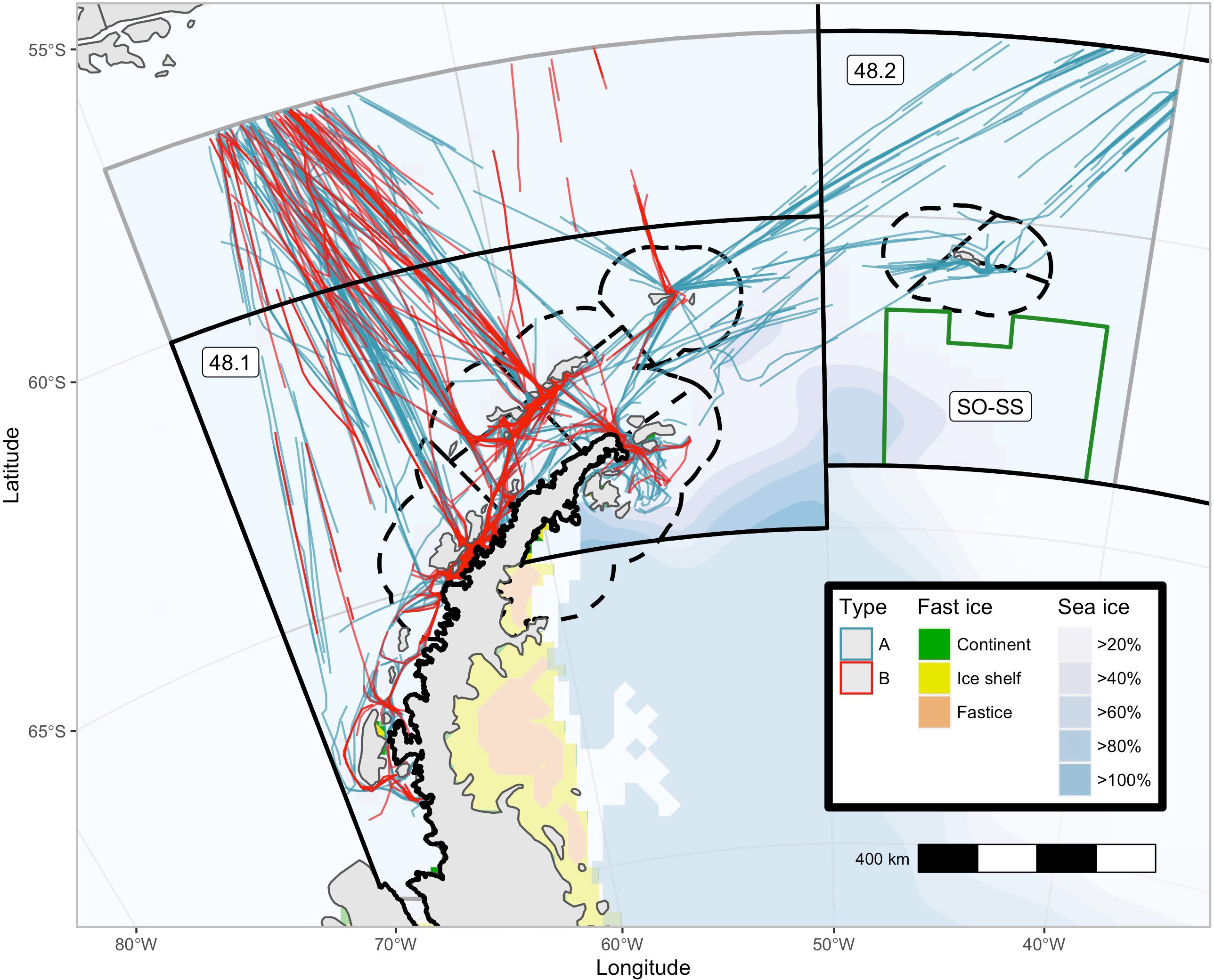
Figure 1 Potential survey effort from a portion of the tourist vessels that tour the southwest Atlantic Ocean (November-March). Modified tourist vessel tracks from 29 of the 45 vessels which toured the southwest Atlantic Ocean in the 2019/20 Antarctic summer tourist season. CCAMLR Management regions Subarea 48.1 and.2 (solid black lines), Small Scale Management Units (dash black lines), and the south Orkney Island Southern Shelf MPA (green line) are plotted. The two basic tourist vessel itineraries are plotted, type (A, B) Sea Ice (extracted from the National Snow and Ice Data Centre via R Package ‘raadtools’) and Fast Ice (Fraser et al., 2020) are as of March 2020.

Estimating the survey effort (km) per tourist vessel-based survey

Automatic identification system (AIS) locations from tourist vessel voyages within the study area from November to March during the 2019/20 austral summer were used to analyze the potential for tourist vessels to make baleen whale observations. This dataset was a subset of the total voyages that the fleet of tourist vessels completed in the western Antarctic Peninsula region in the 2019/20 austral summer season (29 of the 45 tourist vessels and 209 of the total 318 voyages). As vessels report AIS locations at different time frequencies (typically ≈ 500 times/day), the dataset was regularized to hourly locations. To include only locations with appropriate sighting conditions for whale survey, locations with low light conditions (zenith angle of greater than 85°) and average hourly speeds slower than 6 knots or faster than 16 knots were removed (Figure 1). There were two basic voyage plans; (i) voyages that transit from southern Patagonia via South Georgia (and sometimes the South Orkney Islands) before reaching the west Antarctic Peninsula (Type A), and (ii) those that transit directly to the west Antarctic Peninsula, occasionally via the Falkland Islands/Islas Malvinas (Type B). Most vessels complete a variety of voyage plans across a single season.

Additional potential survey effort is lost due to poor weather. The resultant survey effort achieved is termed, realized survey effort (i.e., the survey design minus the sections of track missed due to weather, poor light, etc.). Here, we estimated realized survey effort by correcting the potential survey effort (our ‘survey design’) for expected weather conditions. We then multiplied the estimated realized survey effort by the expected baleen whale sighting rates for the region to estimate the expected number of sightings achieved per voyage.

To estimate the hours of survey effort potentially lost to poor weather we used weather data collected during IWC’s IDCR/SOWER surveys (Branch and Butterworth, 2001b). This dataset was used as it contained a routine hourly collection of weather observations between 0600 and 2000 local time. The proportion of time deemed good weather during IWC’s IDCR/SOWER survey was binned spatially (10˚ Longitude* 2.5˚ Latitude). Good weather was defined as when the sightability score (a measure of sighting conditions on a scale from 1 (poor) – 5 (excellent)) ranged from 3 to 5. Potential survey effort was split to a maximum of 25km lengths, (as is typical for surveys covering ocean basins) and binned spatially (10˚ Longitude* 2.5˚ Latitude). To simulate a dataset of realized survey effort, a random sample was drawn from this split potential survey effort of equivalent size to the proportion of good weather days in that spatial bin (Supplementary Material 1). This was used to estimate the number of kilometers of realized survey effort per voyage (Supplementary Material 2), creating a dataset of realized survey effort segments to sample the simulated whale fields (described below). Note for spatial bins where <10 IWC’s IDCR/SOWER survey-derived hourly weather observations were recorded (colored dark grey in Supplementary Material 2), the mean proportion of good weather hours was used.

Estimating the number of sightings per tourist vessel-based survey

Many Southern Ocean whale species are recovering (Leaper and Miller, 2011; Tulloch et al., 2019), and as such sighting rates of equivalent surveys will also be expected to change commensurately. We define a sighting as an observation of a group of whales from 1 to n individuals (moving together, less than 5 body lengths apart, and only separating temporarily), and a sighting rate as the average number of sightings per distance covered (in this case, per km). We divided the number of sightings of each species by the total distance surveyed for each study. To estimate sighting rates for future summer sampling seasons (i.e., 2022/23), a compound interest rate formula was applied:

$$Sighting rate=(\frac{Recent sighting rate}{Past sighting rate})ˆ((\frac{1}{time period})-1)$$

to estimate the annual rate of change in sighting rates for the period between past (2000) and recent studies (2019) and project into the future (2022/23 season). Past sighting rates were taken from surveys in the year 2000 (The IWC SOWER/CCAMLR krill survey of the year 2000 (Hedley et al., 2001), herein, CCAMLR 2000) and in 2001/02 austral summer (tourist vessel-based survey (Williams, 2003; Williams et al., 2006)). Recent sighting rates were taken from surveys early in the year 2019 (a repeat of the CCAMLR 2000 Survey (Baines et al., 2021), herein, CCAMLR 2019) and the 2018/19 and 2021/22 tourist vessel-based surveys (Johannessen et al., 2022). The spatial range of these studies vary, but all covered the study area at least partially. Sighting rates were calculated separately for the six most common baleen whale species (humpback, fin, Antarctic minke, southern right, sei, and blue) and large unidentified baleen whales (unids). The time period between past and recent surveys was 19 years. The error was not propagated across these estimates due to inconsistent calculation and reporting across the four studies included.

It is reasonable to assume that only small observation teams will be accommodated on tourist vessels, so we assumed a team of two observers per vessel. To maintain consistent observer effort and manage fatigue for a team of this size, the field of observation was restricted to a single observer focused from 0 to 90˚ on one side of the vessel. The second observer would be required to log information on the observational effort, environmental conditions, and animal sightings. Alternative use of two observers was considered, but a 90˚ field of view was considered the best use of a small team of observers. This is because of the limited space allocated on the bridge, the distraction of bridge crew and radio interference due to the high volume of radio chatter between observers on both bridge wings, and occasional super high densities of whales potentially overwhelming observers (Herr et al., 2022). Scientific surveys generally have larger teams on dedicated platforms and can survey the full 180˚ in front of the vessel. To account for this difference in survey design, the final estimated sighting rates for the 2022/23 season were divided by two (where appropriate). Finally, this sighting rate was multiplied by our estimated realized survey effort per voyage to predict the number of sightings per voyage and therefore the voyages required to reach the 60-80 sightings per species for fitting detection functions (Buckland et al., 2001).

Creating simulated whale fields

To understand the extent to which the spatial distribution of the tourist vessel-based survey may bias subsequent model-based abundance estimates, we simulated four whale fields (rasters of whale densities with paired abundances) and sampled them with our dataset of realized survey effort. The four simulated whale fields were created to represent four Southern Ocean foraging baleen whale species: humpback, fin, minke, and blue. Each was generated using rasters of a suite of satellite-derived environmental variables for January 2020 extracted using the R package ‘raadtools’ (Sumner, 2015). For each of the simulated whale fields, a series of environmental variable rasters (n = 3-4) were selected, with paired mean and standard deviation; chosen to reflect previously reported predictors of high densities of the respective baleen whale species in the Southern Ocean (Table 1). Values from a normal distribution (created from the above paired mean and standard deviation) replaced the values in the selected environmental variable rasters. For example, peak humpback whale densities are thought to occur around the 1˚ isotherm (Kasamatsu et al., 2000; Branch, 2011; Johannessen et al., 2022), so all values of 1˚ had the highest density of humpback whales, with decreasing densities towards higher or lower temperatures (SD:1, range: 0-2, Table 1). In this example, sea surface temperature values outside this range (0-2) were assigned a value of 0. A random field was also created for the study area, using the R function ‘sim.rf()’ in package ‘fields’ (Furrer et al., 2009) to incorporate “noise” into the relationship between environmental variables and whale densities by “simulating a stationary Gaussian random field on a regular grid with unit marginal variance” (Furrer et al., 2009). Each of these environmental variable-derived whale fields and the random field were scaled to values of between 0 and 1 (to ensure equal influence), and summed, before being rescaled to reflect probable study area-wide abundance. Simulated whale fields were plotted in Figures 2A–D(i) with tourist vessel-based sampling overlaid, and in Figures 3A–D(i) with scientific vessel-based sampling overlaid.

TABLE 1

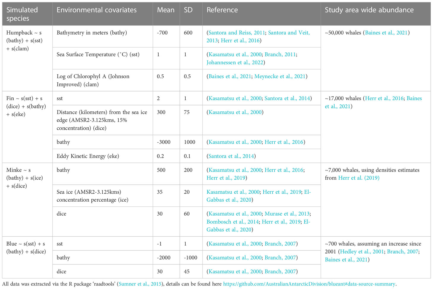
Table 1 Literature sort to determine satellite-derived environmental variables used in creating simulated whale fields.

Sampling simulated whale fields

A total of 6346 sampling segments with a maximum of 25 km transect lengths were derived from 209 voyages. As it is practically unfeasible to sample from 209 voyages in a single summer season, we reduced this dataset to 30 randomly selected voyages, resulting in 974 sampling segments. We used the midpoints of these 974 sampling segments to directly sample our simulated whale density (the observation process was not simulated/recreated). The response variable density was modeled as a function of environmental covariates used to create the simulated whale field, a spatial correlation term (a smooth function of easting and northing) and a Gaussian distribution with a log link using GAMs (i.e., whale.density ~ s(x,y) + s(Enviro 1) + s(Enviro n)+…, Table 1) (using R package ‘mgcv’ (Wood, 2015)). No spatial autocorrelation was introduced into simulated whale fields other than that inherently presented in environmental variables (where values of similar magnitude often occur in adjacent cells). R functions, predict.gam() and dsm_var_gam() (R package ‘dsm’ (Miller et al., 2021)) were used to estimate grid-scale densities and coefficient of variation (CV), and summed to represent modeled abundance. The coefficient of variation associated with the modeled abundance estimate was calculated using the delta method (Ver Hoef, 2012). To provide a comparison to the results achieved with tourist vessel-based sampling, this process was repeated with the true set of realized survey effort achieved during a systematically designed scientific survey, CCAMLR 2019 (Baines et al., 2021) (herein, scientific vessel based-survey). Again, using a maximum segment length of 25km, resulting in 370 sampling segments.

Tourist vessel-based resampling of simulated whale fields

To further our understanding of the relationship between an increasing number of tourist vessel-based surveys (voyages) and the performance of the model (i.e., modeled abundance and associated CV), we compared abundance estimates obtained by six through 30 voyages, each drawn randomly from the dataset. Each of these 25 samples (six-30 voyages) was redrawn randomly from the dataset 40 times, for a total of 1,000 samples. The GAM was fit (relevant to the simulated whale field, Table 1), and modeled abundance and associated CV were calculated. This process was repeated for each of the four simulated whale fields.

All data analysis was conducted in the scientific programming language R (R Core Team, 2021). R packages ‘tidyverse’ (Wickham et al., 2019), ‘sf’ (Pebesma, 2018), ‘raster’ (Hijmans et al., 2013), and ‘ggplot2’ (Wickham, 2011) were used for data manipulation, plotting and analysis.

Results

Estimated length of survey effort per tourist vessel-based survey

After filtering out night and low light locations the 29 vessels covered 279,473 km of potential survey effort with a mean vessel speed of 9.5 knots (range: 0-16, SD: 2.93, SE: ± 0.05) and a mean of 1,293 km per voyage (range: 583-3908, SD: 499, SE: ± 32.9). After allowing for potential weather effects on the sighting conditions, the 29 vessels provided 119,133 km of realized survey effort, or a mean of 551 km per voyage (range: 211-1515, SD: 201, SE: ± 13.7) (Supplementary Material 2). Assuming a strip width of 2 km from a 0 to 90˚ observation field the 29 vessels included in this study could have surveyed a maximum of 15% of the 1.4 million km² study area. On average each voyage would sample 0.078% of the study area (1102 km²), with 18 voyages required for a similar percentage to broad-scale scientific surveys CCAMLR 2000 and 2019 surveys (Table 2).

TABLE 2

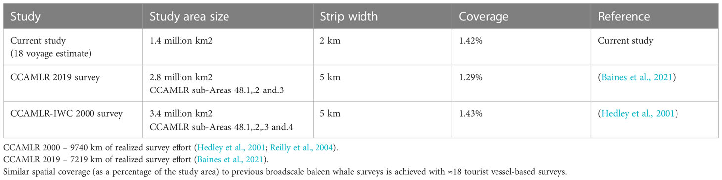
Table 2 Comparisons of the searched area between scientific vessel-based surveys and tourist platform-based surveys.

Estimated sighting rates per tourist vessel-based survey

Expected sighting rates differed by three orders of magnitude among species (range: 0.0002-0.0974 whale sightings/km of survey effort) (Table 3). The annual rate of change in sighting rates over the 19 years was a ~10% increase for humpback, fin, sei, and blue (range: 0.050 - 0.156 whale sightings/km of survey effort) while for Antarctic minke and southern right whales, rates declined by ~5% (range: -0.092 - -0.012 whale sightings/km of survey effort) (Table 3). Sighting rates for large unidentified baleen whales (unids) remained relatively stable (Table 3). Humpback and fin whales are likely to dominate sightings with approximately 26 and 6 sightings predicted per voyage respectively, with a total of 39 baleen whale sightings on average (Table 3). Two-three voyages were needed to estimate detection functions for humpback whales, and 10-13 for fin whales (Table 3). Greater than 30 voyages per season were required for the four other species (Table 3).

TABLE 3

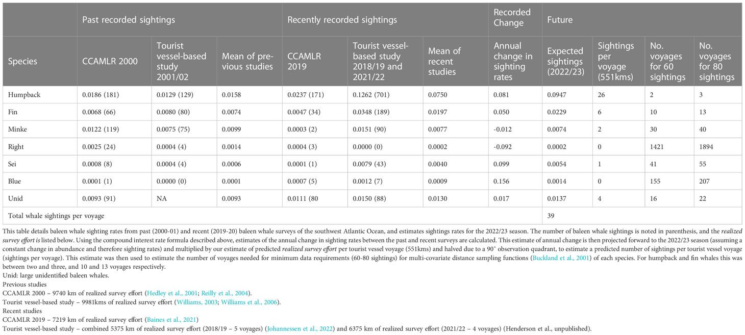
Table 3 Predicted baleen whale sighting rates (whale sightings/kilometer of realized survey effort) for the 2022/23 season calculated from past and recent sighting surveys.

Comparative sampling of simulated whale fields

When using tourist vessel-based sampling, the spatial patterns in the simulated whale fields (Figures 2A–D(i), (ii), (iii), and (iv)) were well reflected in modeled whale abundance (Figures 2A–D(i), (ii), (iii), and (iv)). However, these four models overestimated the simulated whale abundance by approximately 30% (overestimation range: 23-36%, Table 4). Regions where the ‘true’ simulated whale density differed from the modeled whale density (Figures 2A–D(i), (ii), (iii), and (iv)), were generally well highlighted by high grid-scale CV values (Figures 2A–D(i), (ii), (iii), and (iv)), with the possible exception of minke whales (compare Figure 2C(iii) with Figure 2C(iv)), which also had the greatest overestimation in total abundance (36%, Table 4). It appears that when high densities were close to the southern edges of the study region, which was the case for humpback, minke, and blue simulated whale fields, this caused problems for the model, particularly in the western Weddell Sea region (60˚W, Figure 2).

FIGURE 2

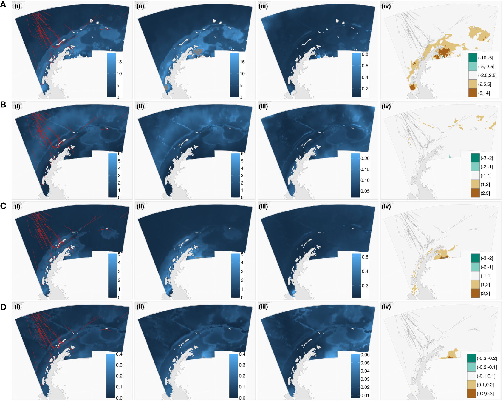
Figure 2 Tourist vessel-based sampling of the humpback (A), fin (B), minke (C), and blue (D) simulated whale fields. Plotted left to right are; (i) the simulated whale field (lighter blues are the higher density of whales) and tourist vessel-based sampling (red lines), (ii) the equivalent modeled whale densities on the same color scale (noting dark grey regions are those where predictions are far greater than the original simulated whale field, see Table 4 for the value ranges), (iii) grid-scale coefficient variations (CV) and, (iv) the true spatiality explicit differences between simulated (i) and modeled (ii) whale fields (scale from greens (underestimate) to white (approximately equal) to browns (overestimated)) with tourist vessel-based sampling (grey lines). These plots show the model generally predicted the spatial patterns in the original simulated whale fields well but performed poorly in some regions (iv). Compare grid-scale CV (iii) with true differences (iv) for inconsistencies between model output and the actual differences between the simulated and modeled grid-scale whale densities.

TABLE 4

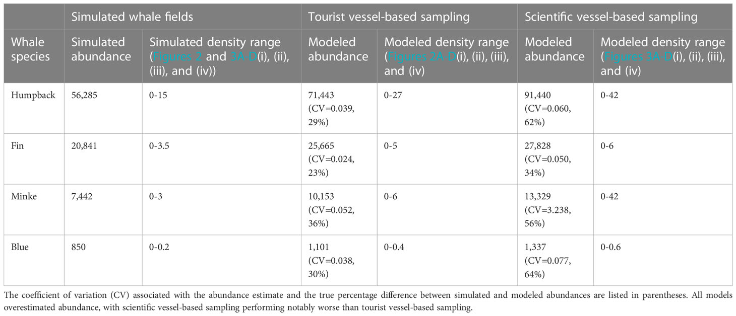
Table 4 Simulated abundance estimates for the four simulated whale fields and their respective modeled abundance estimates (see Table 1 for formulas) from tourist vessel-based and scientific vessel-based sampling.

Scientific vessel-based sampling performed worse at recreating each of the four simulated whale fields, with a higher overestimation of modeled abundance and associated variance (Table 4). Again, models had difficulty in the southern reaches of the study area. Regions where the ‘true’ simulated whale density differed from the modeled whale density (Figures 3A–D(i), (ii), (iii), and (iv)), were generally well highlighted by higher grid-scale CV values (compare Figures 3A–D(iii) with Figure 3A–D(iv))). Note the scales in these plots, dark grey regions in Figures 2 and 3A–D(ii) depict where values were overestimated outside the plotted scale (consistent scales were used across Figures 2 and 3 to accurately depict values).

FIGURE 3

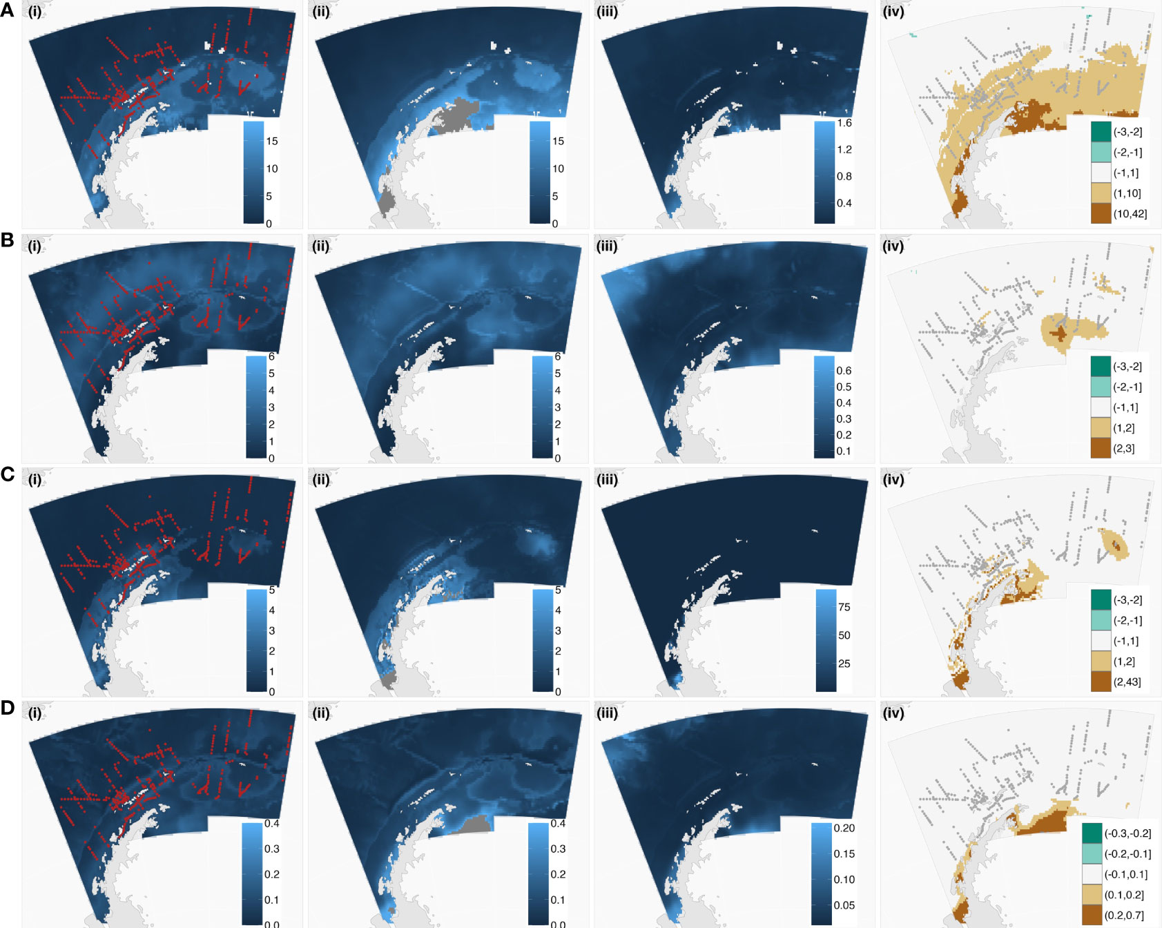
Figure 3 Scientific vessel-based sampling of the humpback (A), fin (B), minke (C), and blue (D) simulated whale fields. Plotted left to right are; (i) the simulated whale field (lighter blues are the higher density of whales) and scientific vessel-based sampling (red lines), (ii) the equivalent modeled whale densities on the same color scale (noting dark grey regions are those where predictions are far greater than the original simulated whale field, see Table 4 for the value ranges), (iii) grid-scale coefficient variations (CV) and, (iv) the true spatiality explicit differences between simulated (i) and modeled (ii) whale fields (scale from greens (underestimate) to white (approximately equal) to browns (overestimated)) with science vessel-based sampling (grey lines). These plots show the model generally predicted the spatial patterns in the original simulated whale fields well but performed poorly in some regions (iv). Compare grid-scale CV (iii) with true differences (iv) for inconsistencies between model output and the actual differences between the simulated and modeled grid-scale whale densities.

In both cases, sampling of the simulated fin whale field (Figure 2D and Figure 3D) fared better than the simulated humpback and minke whale fields (Figure 2A and C and Figure 3A and C) perhaps due to the greater relative densities of simulated whales in the north portion of the study area for fin whales. Full model outputs for each GAM were presented in the supplementary material (Supplementary Material 3). Although this has not been tested here, an exploration into soap film smoothing (Wood et al., 2008), particularly along the convoluted southern edge of the study area may reduce some overestimation of models.

Resampling improved precision and accuracy with increased sample size

The resampling analysis showed model precision (CV) and accuracy (abundance) improved with each additional sample added to the dataset, which is depicted in the reduced spread of values and median of each sample group (six-30 voyages) for both abundance and CV (Figure 4). The median CV within each sample was below 0.25 for all samples but tapered differently between samples. Based on the progressive improvement of precision (CV) and accuracy (abundance), we suggest a sample size of 18-22, 12-16, 17-22, and 13-18 for the humpback, fin, minke, and blue simulated whale fields respectively (grey boxes, Figure 4). For smaller sample sizes there remained substantial improvement in the CV, while for larger sample sizes the improvement was negligible, suggesting an overall sample size of 12-22 voyages. Almost all samples have CVs below 0.25 after ≈18 voyages (except for the humpback whale simulation). Compared to the CV values, abundance values were less variable, with improvements mimicking that of CV values.

FIGURE 4

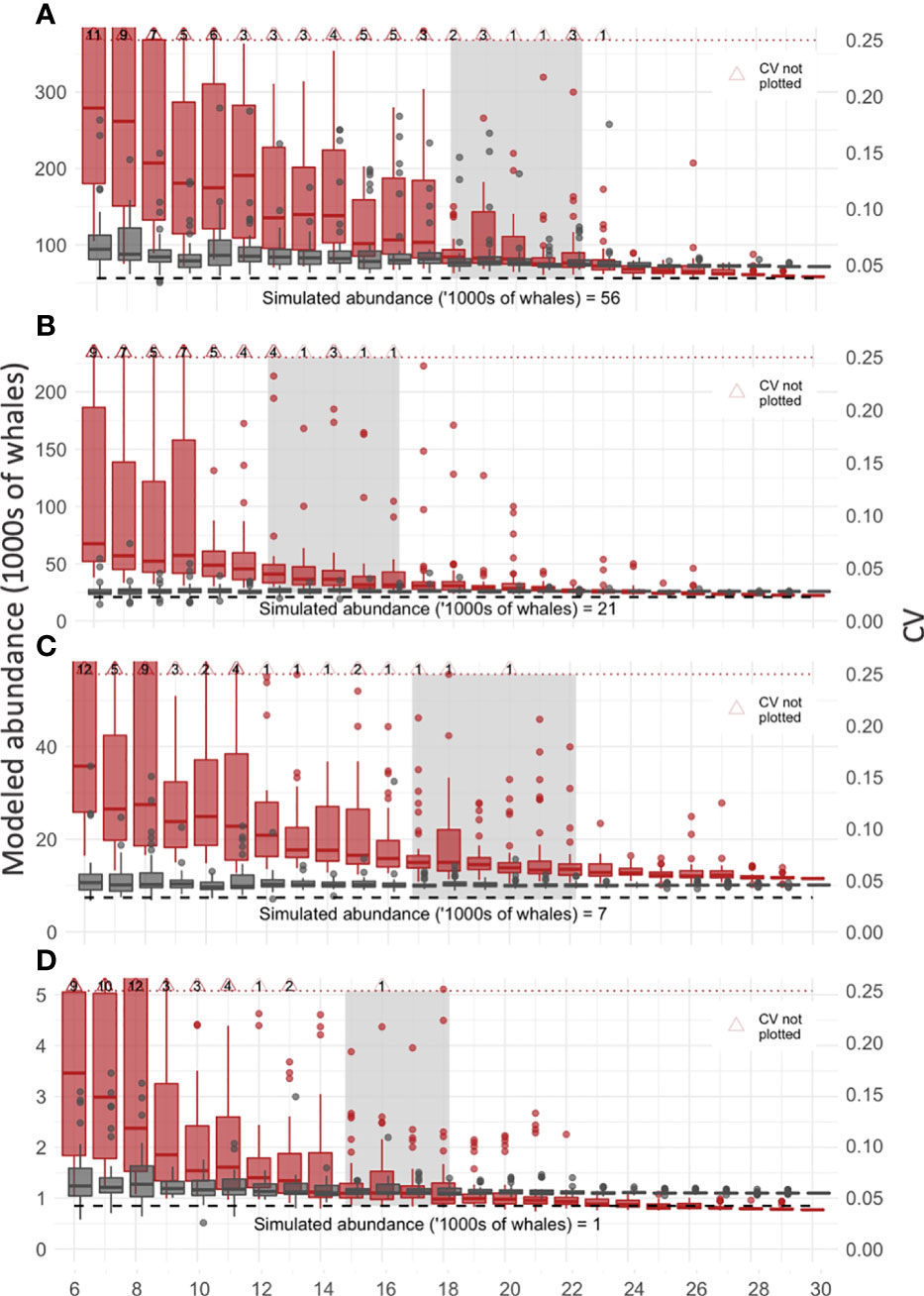
Figure 4 Resampling to detect improvement in precision and accuracy of abundance estimates. The relationship between sample size (number of voyages, x-axis) and improvements in accuracy (modeled abundance, grey boxplots, left y-axis) and precision (CV, red boxplots, right y-axis) are plotted for each of the four simulated whale fields (A-D, humpback, fin, minke, blue respectively). Median values are horizontal lines on boxplots. The upper bound on a useful CV value (0.25, dashed red line) and true simulated whale abundance (dashed black line) are plotted. Light grey boxes mark the sample size, before which CV improves substantially with increased sample size and after which there is negligible improvement in CV. Note these plots are zoomed to exclude some CV values (large red triangles), and the number of values not plotted is noted (black text inside large red triangles).

Discussion

We demonstrate that tourist vessel-based distance sampling surveys have the potential to provide accurate abundance estimates for baleen whales in remote regions. We show that for the southwest Atlantic, 12-22 tourist voyages are likely required to provide an adequate number of sightings to estimate abundance for humpback and fin whales and enable relative approximations of abundance for several other species (as per Reilly et al. (2004); Baines et al. (2021)). We found on average, for each tourist vessel-based baleen whale survey (one voyage) 551km of realized survey effort would be achieved, resulting in 39 baleen whale sightings. Surveys would be dominated by fin and humpback whale sightings. Two-three voyages for humpback whales and 10-13 voyages for fin whales were needed to meet model requirements for abundance estimates. Each tourist vessel-based survey would result in 1102 km² of ocean surveyed, or 0.078% of the study area, suggesting 18 voyages are required to provide similar spatial coverage to earlier science vessel-based baleen whale surveys in the region (1.42%, Table 2, Reilly et al., 2004; Baines et al., 2021). Tourist vessel-based sampling also performed better than scientific vessel-based sampling in estimating whale abundance of simulated whale fields, but still overestimated abundance by approximately 30%. Consequently, the resampling analysis suggested an appropriate sample size of between 12 and 22 voyages.

Potential for inter- and intra-seasonal abundance estimates

The relatively cost-effective nature of tourist vessel-based surveys will allow researchers to repeatedly survey vast regions of the ocean and provide, at minimum, annual estimates of regional abundance for several species of baleen whale. However, given tourist vessels are now operating in the Southern Ocean for more than five months each year, tourist vessel-based survey should also allow intra-annual characterization of abundance, that may capture the spatiotemporal trends in baleen whale movement on foraging grounds (e.g., Johannessen et al., 2022); a fundamental improvement in the data that is currently collected. Currently, most Southern Ocean cetacean surveys aim to detect inter-decadal differences and provide a single abundance estimate from surveys conducted between late December and February (Reilly et al., 2004; Baines et al., 2021) when numbers of baleen whales are thought to be at their maximum (Laws, 1977). This will influence the species composition detected because species arrival on foraging grounds is staggered. Based on whaling records (noting the potential inaccuracies of these data, and the potential changes to baleen whale movement and clustering behavior since whaling) the largest (blue and fin) arrived first followed by humpbacks, then sei and southern right whales much later in the season (February/March) (Mackintosh, 1972). There is also thought to be an inshore and southerly shift of species later in the foraging season around the Antarctic Peninsula, following the contraction of the sea ice (February – June) (Thiele et al., 2004; Johnston et al., 2012; Santora et al., 2014). Neither staggered arrival times nor within-season movement is well captured by current survey efforts, with a recent tourist vessel-based survey illustrating the potential for detecting these trends (Johannessen et al., 2022).

Reliability of modeled abundance estimates derived from tourist ship-based surveys

Tourist vessel-based surveys outperformed the tested scientific vessel-based surveys when sampling our simulated whale fields. When compared to the tourist vessel-based sampling, the relatively worse overestimation of modeled abundance of scientific vessel-based sampling might be because these surveys sample relativity little of the putative high whale density regions in the southern reaches of the survey area. This resulted in an exaggerated spatial smooth (compare contour plots of spatial smooths, Supplementary Material 3). Additionally, scientific vessel-based sampling had a narrower spread of sampled covariate values (compare smoothed covariate plots, noting the x-axis scales vary, Supplementary Material 3). These two constraints (limited sampling of the southern reaches and narrower spread of sampled covariates) likely contributed to the poorer performance of scientific vessel-based sampling and highlight the potential utility of tourist vessel-based sampling.

These simulated examples do not depict real-world whale distributions nor the observation process but do provide real-world examples of sets of circumstances under which models can fail to accurately predict whale densities. Whale densities tend to peak close to the ice edge (Herr et al., 2019) and/or coastal regions for many species (Nowacek et al., 2011; Johnston et al., 2012) which is often the edge of the surveyable study area and potentially punctuated with complex coastal features, characteristics that were all present in the simulated whale fields presented here. Miller and Bravington (2017) describe similar potential real-world examples which can have an almost pathological series of characteristics, causing modeled estimates to deviate substantially from the underlying simulated whale fields. Those presented here contribute to the development of detailed guidelines of best practices for these approaches [as the IWC developed for designed-based surveys (IWC, 2013; Hedley and Bravington, 2014)].

Practical challenges

There are several practical challenges in the use of tourist vessel-based sampling to estimate baleen whale abundance. The most significant of these is ensuring standardization of the data collection process across vessels and observers. The most consistent and replicable observation platform on tourist vessels is likely the bridge; although the field of view will be obstructed by the ship’s superstructure, windows frames, glass, etc. Outside areas on vessels are more problematic as they have uncontrolled tourist interactions with the observer (i.e., alerting observers to sightings) and are inconsistent across vessels. To ensure observers are conducting the observation process in as consistent a manner as possible, the development and implementation of pre-departure training, in-field training, and detailed field protocols in consultation with vessel crews will be required.

These will be passing mode surveys, with no consistent ability to close in on sightings to confirm species identification, group size, etc. Whale approach guidelines for Antarctic tour operators can be found at iaato.org.

Relevance to other regions

This study describes an opportunity for successful engagement with the tourism industry on broad-scale multiday voyages to deliver high-quality scientific outcomes that could benefit the management of living resources in the Southern Ocean. For example, many of the krill-dependent predator groups in the Southern Ocean are monitored as part of the CCAMLR Environmental Monitoring Program (CEMP). However, there remains a large gap in our understanding of baleen whales in this context, with broad-scale monitoring currently occurring only every two decades and no mechanism to include the impact of recovering baleen whale populations on krill stock. The method outlined here appears to be a possible solution for producing annual abundance estimates of baleen whales in the southwest Atlantic Ocean.

There is also potential for the use of tourist ships for surveys of cetaceans and other species (e.g., seals, penguins, and Pelecaniformes seabirds) in other parts of the world, particularly into the Arctic, as many of the same companies operate in both poles. Tourist vessel-based surveys are suited to regions with a relatively high volume of tourist traffic, multiple voyage plans, and low volumes of survey effort from dedicated scientific voyages (Kaschner et al., 2012). In the Arctic, the north Pacific and north Atlantic Ocean sectors appear to be suited (Compton et al., 2007), however further site-specific investigation is needed to determine the viability of achieving robust abundance estimates. Here, the southwest Atlantic region of the Southern Ocean appears to be a viable location for tourist vessel-based surveys, while other regions, such as the Ross Sea and east Antarctica may not be as suitable, due to limited tourist vessel traffic.

There are many examples of coastal vessels being used as ‘platforms of opportunity’ (e.g., tourist, fishing, and cargo vessels and ferries) for collecting scientific data, e.g., marine mammal surveys (Williams et al., 2006; Kiszka et al., 2007; Hupman et al., 2015; Vinding et al., 2015; Viquerat and Herr, 2017) and we now have the statistical tools and computational power to model data from larger spatial areas, across large-scale oceanic regions from multiple tourist vessel platforms. There is potential for a conflict of interests between scientific investigation and vessel operators (e.g., violation of approach distances by tourist vessel operators for enhanced tourist experience (Bearzi, 2017)). However, the success of science and management in resolving complex issues and potential conflicts of interest relies on a holistic approach, such as using social science as a tool for reducing negative wildlife interactions described in Filby et al. (2015); and scientific innovation for reducing seabird bycatch outlined in Avery et al. (2017). Thus, engaging the tourist industry to collect scientific data relevant to management has the potential to result in positive outcomes for all stakeholders; in addition to fostering and incorporating local talent and engaging tourists in the process of science.

Data availability statement

The original contributions presented in the study are included in the article/Supplementary Material, further inquiries can be directed to the corresponding author/s.

Author contributions

This work was conceived by AH, MH, SW, M-AL, NK, and AL. Data provided and curated by MB and AL. Data analysis by AH with support of MH, SW and NK. Drafting of the manuscript by AH, with review from MH, SW, M-AL, MB, NK and AL. All authors contributed to the article and approved the submitted version.

Funding

This work was funded by the Australian Government, Antarctic Science Foundation, and Antarctic Wildlife Research Foundation. In-kind support from University of Tasmania, Australian Antarctic Division, Norwegin Polar Institue, and Insitute of Marine Science.

Conflict of interest

The authors declare that the research was conducted in the absence of any commercial or financial relationships that could be construed as a potential conflict of interest.

The reviewer RL declared a past co-authorship with the author NK to the handling editor.

Publisher’s note

All claims expressed in this article are solely those of the authors and do not necessarily represent those of their affiliated organizations, or those of the publisher, the editors and the reviewers. Any product that may be evaluated in this article, or claim that may be made by its manufacturer, is not guaranteed or endorsed by the publisher.

Supplementary material

The Supplementary Material for this article can be found online at: https://www.frontiersin.org/articles/10.3389/fmars.2023.1048869/full#supplementary-material

Supplementary Material 1 | Spatial binned weather data. The proportion of good weather hours is plotted in spatial bins (10˚ Longitude* 2.5° Latitude) on a continuous gradient scale (lighter blues have a greater proportion of good weather survey conditions). Hourly locations from IWC SOWER surveys from which this weather data was derived are plotted in red. Spatial bins with 0 and<10 weather observations were colored white and grey respectively.

Supplementary Material 2 | Histogram of the length of potential survey effort (km, blue) and estimated realized survey effort (red) per voyage each month (November (A) to March (E) and overall (F). The median for each group is plotted as a vertical line.

Supplementary Material 3 | Model outputs of R package ‘mgcv’ function plot.gam(), and vis.gam() from GAMs in and . These plots are presented in pairs to compare tourist vessel-based sampling with scientific vessel-based sampling.

References

Ainley D. G., Ballard G., Dugger K. M. (2006). Competition among penguins and cetaceans reveals trophic cascades in the Western Ross Sea, Antarctica. Ecology 87, 2080–2093. doi: 10.1890/0012-9658

PubMed Abstract | CrossRef Full Text | Google Scholar

Avery J. D., Aagaard K., Burkhalter J. C., Robinson O. J. (2017). Seabird longline bycatch reduction devices increase target catch while reducing bycatch: A meta-analysis. J. Nat. Conserv. 38, 37–45. doi: 10.1016/j.jnc.2017.05.004

CrossRef Full Text | Google Scholar

Baines M., Kelly N., Reichelt M., Lacey C., Pinder S., Fielding S., et al. (2021). Population abundance of recovering humpback whales megaptera novaeangliae and other baleen whales in the Scotia arc, south Atlantic. Mar. Ecol. Prog. Ser. 676, 77–94. doi: 10.3354/meps13849

CrossRef Full Text | Google Scholar

Baker C. S., Clapham P. J. (2004). Modelling the past and future of whales and whaling. Trends Ecol. Evol. 19, 365–371. doi: 10.1016/j.tree.2004.05.005

PubMed Abstract | CrossRef Full Text | Google Scholar

Bassoi M., Acevedo J., Secchi E. R., Aguayo-Lobo A., Dalla Rosa L., Torres D., et al. (2020). Cetacean distribution in relation to environmental parameters between drake passage and northern Antarctic peninsula. Polar Biol. 43, 1–15. doi: 10.1007/s00300-019-02607-z

CrossRef Full Text | Google Scholar

Bearzi M. (2017). Impacts of marine mammal tourism (Cham: Ecotourism’s promise and peril Springer), 73–96. doi: 10.1007/978-3-319-58331-0_6

CrossRef Full Text | Google Scholar

Bender N. A., Crosbie K., Lynch H. J. (2016). Patterns of tourism in the Antarctic peninsula region: A 20-year analysis. Antarct. Sci. 28, 194–203. doi: 10.1017/S0954102016000031

CrossRef Full Text | Google Scholar

Bombosch A., Zitterbart D. P., Van Opzeeland I., Frickenhaus S., Burkhardt E., Wisz M. S., et al. (2014). Predictive habitat modelling of humpback (Megaptera novaeangliae) and Antarctic minke (Balaenoptera bonaerensis) whales in the southern ocean as a planning tool for seismic surveys. Deep Sea Res. Part Oceanogr. Res. Pap. 91, 101–114. doi: 10.1016/j.dsr.2014.05.017

CrossRef Full Text | Google Scholar

Branch T. A. (2007). Abundance of Antarctic blue whales south of 60 s from three complete circumpolar sets of surveys. J. Cetacean. Res. Manage 9, 253–262.

Google Scholar

Branch T. (2011). Humpback whale abundance south of 60°S from three complete circumpolar sets of surveys. J. Cetacean Res. Manage. Spec. 3, 53–69. doi: 10.47536/jcrm.vi.305

CrossRef Full Text | Google Scholar

Branch T. A., Butterworth D. S. (2001a). Estimates of abundance south of 60°S for cetacean species sighted frequently on the 1978/79 to 1997/98 IWC/IDCR-SOWER sighting surveys. J. Cetacean Res. Manage. 3 (3), 251–270.

Google Scholar

Branch T. A., Butterworth D. S. (2001b). Southern hemisphere minke whales: Standardised abundance estimates from the 1978/79 to 1997/98 IDCR-SOWER surveys. Cetacean Res. Manage. 3 (2), 143–174.

Google Scholar

Buckland S. T., Anderson D. R., Burnham K. P., Laake J. L., Borchers D. L., Thomas L. (2001). Introduction to distance sampling: Estimating abundance of biological populations. Oxford, United Kingdom): Oxford Univ. Press.

Google Scholar

Cañadas A., Hammond P. S. (2008). Abundance and habitat preferences of the short-beaked common dolphin Delphinus delphis in the southwestern Mediterranean: Implications for conservation. Endanger. Species Res. 4 (3), 309–331.

Google Scholar

Carrasco J. F., Bozkurt D., Cordero R. R. (2021). A review of the observed air temperature in the Antarctic peninsula. did the warming trend come back after the early 21st hiatus? Polar Sci. 28, 100653. doi: 10.1016/j.polar.2021.100653

CrossRef Full Text | Google Scholar

Compton R., Banks A., Goodwin L., Hooker S. K. (2007). Pilot cetacean survey of the sub-Arctic north Atlantic utilizing a cruise-ship platform. J. Mar. Biol. Assoc. U. K. 87, 321–325. doi: 10.1017/S0025315407054781

CrossRef Full Text | Google Scholar

El-Gabbas A., Opzeeland I. V., Burkhardt E., Boebel O. (2020). Static species distribution models in the marine realm: The case of baleen whales in the southern ocean. Divers. Distrib 27 (8), 1536–1552. doi: 10.1111/ddi.13300

CrossRef Full Text | Google Scholar

Erbe C., Dähne M., Gordon J., Herata H., Houser D. S., Koschinski S., et al. (2019). Managing the effects of noise from ship traffic, seismic surveying and construction on marine mammals in Antarctica. Front. Mar. Sci. 0. doi: 10.3389/fmars.2019.00647

CrossRef Full Text | Google Scholar

Filby N. E., Stockin K. A., Scarpaci C. (2015). Social science as a vehicle to improve dolphin-swim tour operation compliance? Mar. Policy 51, 40–47. doi: 10.1016/j.marpol.2014.07.010

CrossRef Full Text | Google Scholar

Fraser A. D., Massom R. A., Ohshima K. I., Willmes S., Kappes P. J., Cartwright J., et al. (2020). High-resolution mapping of circum-Antarctic landfast sea ice distribution 2000–2018. Earth Syst. Sci. Data 12, 2987–2999. doi: 10.5194/essd-12-2987-2020

CrossRef Full Text | Google Scholar

Furrer R., Nychka D., Sain S., Nychka M. D. (2009). Package ‘fields.’ r found. stat. comput (Vienna Austria).

Google Scholar

Hedley S., Bravington M. (2014). “Comments on design-based and model-based abundance estimates for the RMP and other contexts,” in Paper SC/65b/RMP11 presented to the 65b IWC Scientific Committee, , May 2014. 9.

Google Scholar

Hedley S., Reilly S., Borberg J., Holland R., Hewitt R., Watkins J., et al. (2001). “Modelling whale distribution: A preliminary analysis of data collected on the CCAMLR-IWC krill synoptic surve,” in Paper SC/53/E9 presented to the 54th Meeting of the International Whaling Commission, , July 2001.

Google Scholar

Herr H., Viquerat S., Devas F., Lees A., Wells L., Gregory B., et al. (2022). Return of large fin whale feeding aggregations to historical whaling grounds in the Southern Ocean. Sci. Rep. 12, 9458. doi: 10.1038/s41598-022-13798-7

PubMed Abstract | CrossRef Full Text | Google Scholar

Herr H., Kelly N., Dorschel B., Huntemann M., Kock K.-H., Lehnert L. S., et al. (2019). Aerial surveys for Antarctic minke whales (Balaenoptera bonaerensis) reveal sea ice dependent distribution patterns. Ecol. Evol. 9, 5664–5682. doi: 10.1002/ece3.5149

PubMed Abstract | CrossRef Full Text | Google Scholar

Herr H., Viquerat S., Siegel V., Kock K.-H., Dorschel B., Huneke W. G. C., et al. (2016). Horizontal niche partitioning of humpback and fin whales around the West Antarctic peninsula: evidence from a concurrent whale and krill survey. Polar Biol. 39, 799–818. doi: 10.1007/s00300-016-1927-9

CrossRef Full Text | Google Scholar

Hijmans R. J., van Etten J., Mattiuzzi M., Sumner M., Greenberg J. A., Lamigueiro O. P., et al. (2013). Raster package in r. version.

Google Scholar

Horton T. W., Palacios D. M., Stafford K. M., Zerbini A. N. (2022). “Baleen whale migration,” in Ethology and behavioral ecology of mysticetes. ethology and behavioral ecology of marine mammals. Eds. Clark C. W., Garland E. C. (Cham: Springer). doi: 10.1007/978-3-030-98449-6_4

CrossRef Full Text | Google Scholar

Hupman K., Visser I., Martinez E., Stockin K. (2015). Using platforms of opportunity to determine the occurrence and group characteristics of orca (Orcinus orca) in the hauraki gulf, new Zealand. N. Z. J. Mar. Freshw. Res. 49, 132–149. doi: 10.1080/00288330.2014.980278

CrossRef Full Text | Google Scholar

International Association of Antarctic Tour Operators Overview of Antarctic tourism: A historical review of growth, the 2020-21 season, and preliminary estimates for 2021-22. Available at: https://iaato.org/wp-content/uploads/2021/07/ATCM43_ip110_e.docx (Accessed 14-May-2021).

Google Scholar

International Whaling Commission (2013). Reports of the subcommittee on in-depth assessments. J. Cetacean Res. Manage. 14 (Suppl.), 195–213.

Google Scholar

Johannessen J. E. D., Biuw M., Lindstrøm U., Ollus V. M. S., Martín López L. M., Gkikopoulou K. C., et al. (2022). Intra-season variations in distribution and abundance of humpback whales in the West Antarctic peninsula using cruise vessels as opportunistic platforms. Ecol. Evol. 12, e8571. doi: 10.1002/ece3.8571

PubMed Abstract | CrossRef Full Text | Google Scholar

Johnston D., Friedlaender A., Read A., Nowacek D. (2012). Initial density estimates of humpback whales megaptera novaeangliae in the inshore waters of the western Antarctic peninsula during the late autumn. Endanger. Species Res. 18, 63–71. doi: 10.3354/esr00395

CrossRef Full Text | Google Scholar

Kasamatsu F., Matsuoka K., Hakamada T. (2000). Interspecific relationships in density among the whale community in the Antarctic. Polar Biol. 23, 466–473. doi: 10.1007/s003009900107

CrossRef Full Text | Google Scholar

Kaschner K., Quick N. J., Jewell R., Williams R., Harris C. M. (2012). Global coverage of cetacean line-transect surveys: Status quo, data gaps and future challenges. PloS One 7, e44075. doi: 10.1371/journal.pone.0044075

PubMed Abstract | CrossRef Full Text | Google Scholar

Kawaguchi S., Nicol S. (2020). Krill fishery. Fish Aquac 9, 137. doi: 10.1093/oso/9780190865627.003.0006

CrossRef Full Text | Google Scholar

Kiszka J., Macleod K., Van Canneyt O., Walker D., Ridoux V. (2007). Distribution, encounter rates, and habitat characteristics of toothed cetaceans in the bay of Biscay and adjacent waters from platform-of-opportunity data. ICES J. Mar. Sci. 64, 1033–1043. doi: 10.1093/icesjms/fsm067

CrossRef Full Text | Google Scholar

Laws R. M. (1977). Seals and whales of the southern ocean. Philos. Trans. R. Soc Lond. B Biol. Sci. 279, 81–96.

Google Scholar

Leaper R., Miller C. (2011). Management of Antarctic baleen whales amid past exploitation, current threats and complex marine ecosystems. Antarct. Sci. 23, 503–529. doi: 10.1017/S0954102011000708

CrossRef Full Text | Google Scholar

Lin Y., Moreno C., Marchetti A., Ducklow H., Schofield O., Delage E., et al. (2021). Decline in plankton diversity and carbon flux with reduced sea ice extent along the Western Antarctic peninsula. Nat. Commun. 12, 4948. doi: 10.1038/s41467-021-25235-w

PubMed Abstract | CrossRef Full Text | Google Scholar

Lynch H. J., Crosbie K., Fagan W. F., Naveen R. (2010). Spatial patterns of tour ship traffic in the Antarctic peninsula region. Antarct. Sci. 22, 123–130. doi: 10.1017/S0954102009990654

CrossRef Full Text | Google Scholar

Mackintosh N. A. (1972). Biology of the populations of large whales. Sci. Prog. 1933- 60, 449–464.

Google Scholar

Marques F. F. C., Buckland S. T. (2003). Incorporating covariates into standard line transect analyses. Biometrics 59, 924–935. doi: 10.1111/j.0006-341X.2003.00107.x

PubMed Abstract | CrossRef Full Text | Google Scholar

McMahon K. W., Michelson C. I., Hart T., McCarthy M. D., Patterson W. P., Polito M. J. (2019). Divergent trophic responses of sympatric penguin species to historic anthropogenic exploitation and recent climate change. Proc. Natl. Acad. Sci. 116, 25721–25727. doi: 10.1073/pnas.1913093116

CrossRef Full Text | Google Scholar

Meynecke J.-O., de Bie J., Barraqueta J.-L. M., Seyboth E., Dey S. P., Lee S. B., et al. (2021). The role of environmental drivers in humpback whale distribution, movement and behavior: A review. Front. Mar. Sci. 8. doi: 10.3389/fmars.2021.720774

CrossRef Full Text | Google Scholar

Miller D. L., Bravington M. V. (2017). “When can abundance surveys be analysed with “design-based” methods?,” in Paper SC/67B/NH/04 presented to the 67th Meeting of the International Whaling Commission, , September 2018.

Google Scholar

Miller D. L., Burt M. L., Rexstad E. A., Thomas L. (2013). Spatial models for distance sampling data: Recent developments and future directions. Methods Ecol. Evol. 4, 1001–1010. doi: 10.1111/2041-210X.12105

CrossRef Full Text | Google Scholar

Miller D. L., Rexstad E., Burt L., Bravington M. V., Hedley S., Model A. (2021). Package ‘dsm.’.

Google Scholar

Murase H., Kitakado T., Hakamada T., Matsuoka K., Nishiwaki S., Naganobu M. (2013). Spatial distribution of Antarctic minke whales (Balaenoptera bonaerensis) in relation to spatial distributions of krill in the Ross Sea, Antarctica. Fish. Oceanogr. 22, 154–173. doi: 10.1111/fog.12011

CrossRef Full Text | Google Scholar

Nowacek D. P., Friedlaender A. S., Halpin P. N., Hazen E. L., Johnston D. W., Read A. J., et al. (2011). Super-aggregations of krill and humpback whales in Wilhelmina bay, Antarctic peninsula. PloS One 6, e19173. doi: 10.1371/journal.pone.0019173

PubMed Abstract | CrossRef Full Text | Google Scholar

Palmowski T. (2020). Development of Antarctic tourism. Geoj Tour Geosites 33, 1520–1526. doi: 10.30892/gtg.334spl11-602

CrossRef Full Text | Google Scholar

Pebesma E. J. (2018). Simple features for r: Standardized support for spatial vector data. R J. 10 (1), pp.439–pp.446. doi: 10.32614/RJ-2018-009

CrossRef Full Text | Google Scholar

Ratnarajah L., Bowie A. R., Lannuzel D., Meiners K. M., Nicol S. (2014). The biogeochemical role of baleen whales and krill in southern ocean nutrient cycling. PloS One 9, e114067. doi: 10.1371/journal.pone.0114067

PubMed Abstract | CrossRef Full Text | Google Scholar

Ratnarajah L., Melbourne-Thomas J., Marzloff M. P., Lannuzel D., Meiners K. M., Chever F., et al. (2016). A preliminary model of iron fertilisation by baleen whales and Antarctic krill in the southern ocean: Sensitivity of primary productivity estimates to parameter uncertainty. Ecol. Model. 320, 203–212. doi: 10.1016/j.ecolmodel.2015.10.007

CrossRef Full Text | Google Scholar

R Core Team (2021). R: A language and environment for statistical computing. R Foundation for Statistical Computing, Vienna, Austria. Available at: https://www.Rproject.org/.

Google Scholar

Reilly S., Hedley S., Borberg J., Hewitt R., Thiele D., Watkins J., et al. (2004). Biomass and energy transfer to baleen whales in the south Atlantic sector of the southern ocean. Deep Sea Res. Part II Top. Stud. Oceanogr. 51, 1397–1409. doi: 10.1016/j.dsr2.2004.06.008

CrossRef Full Text | Google Scholar

Santora J. A., Reiss C. S. (2011). Geospatial variability of krill and top predators within an Antarctic submarine canyon system. Mar. Biol. 158, 2527–2540. doi: 10.1007/s00227-011-1753-0

CrossRef Full Text | Google Scholar

Santora J. A., Schroeder I. D., Loeb V. J. (2014). Spatial assessment of fin whale hotspots and their association with krill within an important Antarctic feeding and fishing ground. Mar. Biol. 161, 2293–2305. doi: 10.1007/s00227-014-2506-7

CrossRef Full Text | Google Scholar

Santora J., Veit R. (2013). Spatiotemporal persistence of top predator hotspots near the Antarctic Peninsula. Mar. Ecol. Prog. Ser 487, 287–304. doi: 10.3354/meps10350

CrossRef Full Text | Google Scholar

Savoca M. S., Czapanskiy M. F., Kahane-Rapport S. R., Gough W. T., Fahlbusch J. A., Bierlich K. C., et al. (2021). Baleen whale prey consumption based on high-resolution foraging measurements. Nature 599, 85–90. doi: 10.1038/s41586-021-03991-5

PubMed Abstract | CrossRef Full Text | Google Scholar

Strindberg S., Buckland S. T. (2004). Zigzag survey designs in line transect sampling. J. Agricultural Biol. Environ. Stat 9, 443–461. doi: 10.1198/108571104X15601

CrossRef Full Text | Google Scholar

Sumner M. D. (2015). Raadtools: Tools for synoptic environmental spatial data. r package version 0.5, Vol. 3. 9001, (2020).

Google Scholar

Thiele D., Chester E. T., Moore S. E., Širovic A., Hildebrand J. A., Friedlaender A. S. (2004). Seasonal variability in whale encounters in the Western Antarctic peninsula. Deep Sea Res. Part II Top. Stud. Oceanogr. 51, 2311–2325. doi: 10.1016/j.dsr2.2004.07.007

CrossRef Full Text | Google Scholar

Thomas L., Buckland S. T., Rexstad E. A., Laake J. L., Strindberg S., Hedley S. L., et al. (2010). Distance software: design and analysis of distance sampling surveys for estimating population size. J. Appl. Ecol. 47, 5–14. doi: 10.1111/j.1365-2664.2009.01737.x

PubMed Abstract | CrossRef Full Text | Google Scholar

Thomas L., Williams R., Sandilands D. (2007). Designing line transect surveys for complex survey regions. J. Cetacean Res. Manage. 9, 1–13.

Google Scholar

Tin T., Fleming Z. L., Hughes K. A., Ainley D. G., Convey P., Moreno C. A., et al. (2009). Impacts of local human activities on the Antarctic environment. Antarct. Sci. 21, 3–33. doi: 10.1017/S0954102009001722

CrossRef Full Text | Google Scholar

Tin T., Lamers M., Liggett D., Maher P. T., Hughes K. A. (2014). “Setting the scene: Human activities, environmental impacts and governance arrangements in Antarctica,” in Antarctic Futures. Eds. Tin T., Liggett D., Maher P. T., Lamers M. (Dordrecht: Springer Netherlands), 1–24. doi: 10.1007/978-94-007-6582-5_1

CrossRef Full Text | Google Scholar

Trivelpiece W. Z., Hinke J. T., Miller A. K., Reiss C. S., Trivelpiece S. G., Watters G. M. (2011). Variability in krill biomass links harvesting and climate warming to penguin population changes in Antarctica. Proc. Natl. Acad. Sci. 108, 7625–7628. doi: 10.1073/pnas.1016560108

CrossRef Full Text | Google Scholar

Tulloch V. J. D., Plagányi É.E., Brown C., Richardson A. J., Matear R. (2019). Future recovery of baleen whales is imperiled by climate change. Glob. Change Biol. 25, 1263–1281. doi: 10.1111/gcb.14573

CrossRef Full Text | Google Scholar

Ver Hoef J. M. (2012). Who invented the delta method? Am. Statistician 66, 124–127. doi: 10.1080/00031305.2012.687494

CrossRef Full Text | Google Scholar

Vinding K., Bester M., Kirkman S. P., Chivell W., Elwen S. H. (2015). The use of data from a platform of opportunity (whale watching) to study coastal cetaceans on the southwest coast of south Africa. Tour. Mar. Environ. 11, 33–54. doi: 10.3727/154427315X14398263718439

CrossRef Full Text | Google Scholar

Viquerat S., Herr H. (2017). Mid-summer abundance estimates of fin whales (Balaenoptera physalus) around the south Orkney islands and elephant island. Endanger. Species Res. 32, 515–524. doi: 10.3354/esr00832

CrossRef Full Text | Google Scholar

Warwick-Evans V., A Santora J., Waggitt J. J., Trathan P. N. (2021). Multi-scale assessment of distribution and density of procellariiform seabirds within the northern Antarctic peninsula marine ecosystem. ICES J. Mar. Sci. 78 (4), 1324–1339. doi: 10.1093/icesjms/fsab020

CrossRef Full Text | Google Scholar

Wickham H. (2011). ggplot2. Wiley Interdiscip. Rev. Comput. Stat. 3, 180–185.

Google Scholar

Wickham H., Averick M., Bryan J., Chang W., McGowan L. D., François R., et al. (2019). Welcome to the tidyverse. J. Open Source Software 4, 1686. doi: 10.21105/joss.01686

CrossRef Full Text | Google Scholar

Williams R. (2003). Cetacean studies using platforms of opportunity. unpublished PhD thesis in biology. Univ. St Andrews St Andrews Scotl. UK 238.

Google Scholar

Williams R., Hedley S. L., Hammond P. S. (2006). Modeling distribution and abundance of Antarctic baleen whales using ships of opportunity. Ecol. Soc. 11 (1). doi: 10.5751/ES-01534-110101

CrossRef Full Text | Google Scholar

Williams R., Thomas L. (2009). Cost-effective abundance estimation of rare marine animals: Small-boat surveys for killer whales in British Columbia, Canada. Biol. Conserv. 142, 1542–1547. doi: 10.1016/j.biocon.2008.12.028

CrossRef Full Text | Google Scholar

Wood S. (2015). Package ‘mgcv.’ r package version, 1. 729.

Google Scholar

Wood S. N., Bravington M. V., Hedley S. L. (2008). Soap film smoothing. J. R. Stat. Soc Ser. B Stat. Methodol. 70, 931–955. doi: 10.1111/j.1467-9868.2008.00665.x

CrossRef Full Text | Google Scholar