Improved accuracy and spatial resolution for bio-logging-derived chlorophyll a fluorescence measurements in the Southern Ocean

1 Introduction

Primary producers are key elements in the structuring of marine food webs and their distribution in the ocean largely drives ecosystem dynamics (Lévy et al., 2018; Henley et al., 2020). Primary production also plays a critical role in biogeochemical cycles given its involvement in CO₂ sequestration through the process of the biological carbon pump (DeVries et al., 2012; Siegel et al., 2014; Boyd et al., 2019). Resolving phytoplankton distribution in the ocean is however a challenging issue due to the extreme heterogeneity of environmental conditions and the short time scales of events relative to phytoplankton growth. From the mesoscale (O(100 km)) to the submesoscale (O(10 km)), the oceanic landscape is shaped by dynamic processes such as filaments or eddies which directly impact phytoplankton distribution (Mahadevan, 2016; Lévy et al., 2018). Complex shapes and high patchiness, observable from space with ocean-color radiometry, result from these processes (d’Ovidio et al., 2010; Lehahn et al., 2018), with consequences on the variability of the associated biogeochemical processes (Resplandy et al., 2009).

Remote sensing of ocean-color enables monitoring of the distribution of chlorophyll a (Chla hereafter), a proxy for phytoplankton biomass, with the advantage of providing a synoptic view of the processes occurring at the surface of the ocean. Yet the reflectance signal upcoming from the ocean surface is subject to obstruction by clouds or masking by sea ice (at high latitudes), which requires coupling satellite data with in-situ sampling. Furthermore, the critical need for collecting in-situ data is reinforced by the fact that the vertical distribution of Chla escapes remote detection. Indeed, ocean-color measurements are restricted to the near-surface. Satellite observations consequently only include part of the productive layer and omit potential subsurface features (e.g. deep chlorophyll maxima, see Baldry et al., 2020; Cornec et al., 2021).

While the mesoscale is quite well covered by current satellite observations of physical dynamics coupled with in-situ platforms sampling biogeochemical variables (McGillicuddy, 2016), recent missions like the Surface Water and Ocean Topography (SWOT) mission enable access to spatial scales down to 15-30 km (Morrow et al., 2019) but there is no in-situ counterpart to support the remotely-sensed observations (d’Ovidio et al., 2019). Phytoplankton distribution at submesoscale is hence inadequately resolved due to the gap between satellite observations and in-situ data.

One region where an enhanced submesoscale observation of phytoplankton distribution would be particularly valuable is the Southern Ocean (SO). Considered as a main contributor to global air-sea CO₂ exchange (Ardyna et al., 2017; Bushinsky et al., 2019; De Vries et al., 2019), the SO hosts a large variety of ecosystems, from unicellular organisms up to charismatic megafauna, that rely greatly on ocean biogeochemistry (Deppeler and Davidson, 2017; Henley et al., 2020). In addition to displaying marked seasonal and regional features (Blain et al., 2008; Deppeler and Davidson, 2017), the spatio-temporal variability of phytoplankton concentration in the SO is subject to the heavy structuring effect of the (sub)mesoscale (Bachman et al., 2017) and is strongly influenced by sub-seasonal forcings (Prend et al., 2022). Monitoring the distribution of phytoplankton at such short spatial and temporal scales is therefore crucial. However the monitoring of primary production in the SO through in-situ sampling by research vessels is highly limited by harsh meteorological conditions and by the presence of sea ice. In addition, satellite-based observations in the SO are frequently restricted by cloud coverage. As a result, despite the preeminent position of the SO in the Earth’s climate system and ecosystem functioning, it remains undersampled compared to other ocean basins.

The limitations associated with research vessel-based sampling in the SO lead to opting for autonomous measuring platforms like AUVs (Autonomous Underwater Vehicles). However, both the large extent and the remoteness of the zone highly constrain any AUV deployment and recovery. Nonetheless, large efforts have been made in the past two decades to increase the number of autonomous platforms monitoring the SO through the measurement of biogeochemical variables (Chai et al., 2020). While Biogeochemical-Argo (BGC-Argo) floats enable the sampling of a region over several years (Claustre et al., 2020), gliders (Testor et al., 2019) and marine mammals equipped with bio-logging devices (Blain et al., 2013; Guinet et al., 2013; Treasure et al., 2017) are more suitable for the observation of short-lived (sub)mesoscale processes. Gliders are indisputably a powerful tool for characterizing phytoplankton distribution at these scales due to the high spatio-temporal density they can achieve in the sampling (0.5–6 km, 0.5–6 h between 2 vertical profiles, Rudnick et al., 2016; Testor et al., 2019). However, despite some examples of successful glider deployments in the SO providing an insight into phytoplankton distribution at high resolution (e.g. Kahl et al., 2010), high-frequency data remain rare in the SO because of the deployment constraints mentioned above. By comparison, bio-logging devices mounted on deep-diving animals such as southern elephant seals (Mirounga leonina, SES hereafter) offer the possibility of acquiring as many as 60 profiles per day at depths regularly exceeding 500 m (Siegelman et al., 2019b). Bio-logging devices hence have the potential to address the (sub)mesoscale sampling issue in zones as remote and turbulent as the SO.

The Satellite Relayed Data Logger (SRDL, see Boehme et al., 2009) developed by the Sea Mammal Research Unit (SMRU, UK) is a bio-logging device designed for marine mammals like the SES. SRDLs commonly include a Conductivity, Temperature and Depth (CTD) sensor head. Optionally, SRDLs may include a light sensor, and a fluorometer to measure Chla fluorescence (Fluo hereafter). SRDLs can also act as high-frequency sampling loggers which need to be recovered when the SESs are back ashore in order to obtain access to the data. The present study focuses on SRDLs (referred to as “tags” hereafter) measuring light (L hereafter) and Fluo. Although High Pressure Liquid Chromatography (HPLC) is the reference technique for accurate Chla concentration estimates ([Chla], mg.m^-3) (Wright et al., 1991; Ras et al., 2008), it requires the collection of water samples whereas fluorometers provide a real-time estimate of in-situ [Chla]. Due to their ease of use and the relative simplicity of their integration, fluorescence-based sensors have recently been largely implemented in autonomous platforms. As a consequence, Fluo has become a universal standard variable for the estimate of [Chla]. The measurement of Fluo is based on the optical properties of the Chla photosynthetic pigments present in the sampled water volume (Lorenzen, 1966; Huot and Babin, 2010; Roesler and Barnard, 2013). Fluo is at first order proportional to [Chla]. However, more precise examinations of the Fluo signal reveal that the relationship between the observed fluorescence and the actual phytoplankton biomass can vary according to phytoplankton community composition, physiological factors or light conditions (Serôdio and Lavaud, 2011; Xing et al., 2012; Roesler et al., 2017; Schallenberg et al., 2022). Fluo is hence an imperfect proxy which does not straightforwardly reflect phytoplankton concentration, but remains to date the best means to obtain widespread estimates of in-situ [Chla].

Previous studies have already shown that Fluo data quality can be enhanced by the use of concomitant radiometric measurements, and vice versa (Morel and Maritorena, 2001; Morel et al., 2007; Xing et al., 2011). These methods rely on the hypothesis that light absorption in the water column is mainly due to the presence of phytoplankton. Such a hypothesis is commonly made for oceanic waters with no direct terrestrial influence, classified as “case 1” waters (Morel and Prieur, 1977; Morel, 1988). Based on the same hypothesis but more specifically for inference purposes in the framework of functional data analysis, it has been proved that the vertical diffuse attenuation coefficient for L (K_L hereafter) can be a good predictor for Fluo (Bayle et al., 2015). In the present study we propose to exploit the predictive capabilities of a linear functional model (LFM) similar to the one described by Bayle et al. (2015) (who limited their analysis to the inference of low resolution Fluo data) to adjust the (uncalibrated) Fluo data provided by multiple tags (18 in our study). The tags’ intercalibration does not resolve the issue of the absolute Fluo to [Chla] conversion. Consequently, following the merging of all the intercalibrated tags, we have selected [Chla] estimated by ocean-color radiometry as the benchmark to carry out absolute Fluo calibration.

Another key issue regarding Fluo measurements in the context of bio-logging is related to energy consumption. Not only is energy consumption a major concern for autonomous platforms in general but Fluo measurements are also particularly energy-demanding as they rely on an active optical sensor. The issue is especially critical for bio-logging tags due to the reduced size of such loggers and therefore the highly limited volume of their batteries. A trade-off between the vertical and temporal resolutions of the acquisitions is necessary to best optimize battery lifetime. As a consequence, despite the high sampling resolution of the tags enabled by SES diving behavior (up to ~60 dives per day), suitable for the observation of submesoscale processes, the spatial resolution of the SRDL’s Fluo measurements was reduced (~4 profiles per day) and becomes insufficient for a proper description of phytopankton distribution at that scale. To address this observation gap, a LFM was designed to infer [Chla] from K_L and increase the resolution of the [Chla] field description towards the submesoscale.

To summarize, the method developed in the present study aims at enhancing the quality of the [Chla] estimates provided by a set of multiple SRDLs in terms of accuracy and horizontal resolution through the use of K_L derived from vertical light profiles, combined with satellite estimates of [Chla]. The objective of the present study is to propose and to validate a method based on bio-logging SRDL data to retrieve (1) a calibrated measurement of in-situ [Chla] (2) at submesoscale (O(10 km)). The main steps of the method described in the present study are summarized in Figure 1. An application of the method is presented with the data from two tags deployed in the Kerguelen Islands region.

FIGURE 1

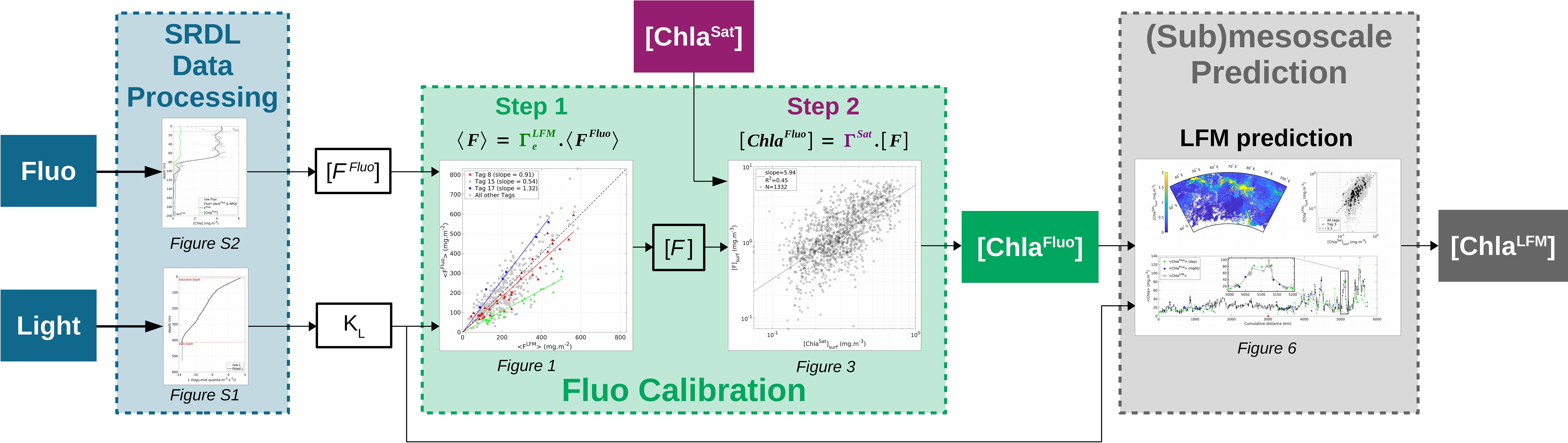
Figure 1 Flowchart summarizing the main steps of the method described in the present study. The method aims at enhancing the quality of the in-situ [Chla] estimates provided by a set of multiple bio-logging devices (SRDLs) in terms of accuracy and horizontal resolution. Based on SRDL data (Fluo and L in-situ measurements, blue boxes) combined with concomitant satellite estimates of [Chla] ([Chla^Sat], purple box), the method firstly enables the constitution of calibrated datasets of in-situ [Chla] estimates ([Chla^Fluo], green box). The method then extends the description of the [Chla] field to (sub)mesoscale ([Chla^LFM], gray box) through the use of K_L as a predictor for [Chla].

2 Material and methods

2.1 Tag data

The present analysis is based on the data from 18 tags deployed on female SESs in the Kerguelen Islands region. The study area is located in the Indian sector of the SO and extends from 43°S to 62°S and from 35°E to 101°E. The 18 tags were deployed during the SESs’ post-breeding foraging trip, which occurs from October of year N to January of year N + 1. In the present study, post-breeding deployments from years 2018 to 2020 were analyzed, totaling 89 197 vertical profiles (for detailed metadata per tag, see supplementary material, Table S1).

The tags were glued on the fur of the SESs’ head using a two component industrial epoxy (see McMahon et al., 2008; Boehme et al., 2009 for animal capture and tag attachment details). After their post-breeding foraging trip, the female SESs were located, recaptured and the tags were retrieved. The tags measure and record pressure (dbar), temperature (°C), salinity (dimensionless), L (μmol quanta.m^-2.s^-1) and Fluo (mg.m^-3) at 0.5 Hz (note that the different variables used in this study and their associated symbols, definitions and units are detailed in Table 1). The tags’ sensor data were continuously sampled during the SESs’ trip, with the exception of the Fluo sensor, which was intermittently switched off to save battery power (see details in Section 2.2.3). The archived time series were processed to produce only one vertical profile per dive, corresponding to the ascent phase of the dive, starting from the deepest part of the dive (down to ~1000 m depth), up to the surface. The SRDL data were interpolated at 1 m resolution. The vertical resolution of 1 m is consistent with the sampling rate of the tags (0.5 Hz) and the vertical speed of the SES during the ascent (~1.5 m.s^-1, see Richard et al., 2014; McGovern et al., 2019).

TABLE 1

Table 1 Acronyms, definitions and units.

For each surfacing phase (i.e. each time the animal emerges to breathe), when available, the location of the animal was recorded, using by default the Argos satellite system, operated by Collecte Localisation Satellites (CLS). When no positioning was transmitted, the location was a posteriori estimated by linearly interpolating the trajectory of the animal. During the interpolation process, the horizontal speed of the animal was taken into account to ensure the spatio-temporal coherency of the location data. Ten of the studied SESs were also equipped with a biometric sonar and movement tag (DTAG). The DTAG placed on the animal’s head picks up the GPS position using the Snapshot GPS acquisition algorithm (Goulet et al., 2019) and enables a more accurate GPS positioning of the profiles than with the Argos system. The positioning accuracy is 2-3 km for Argos, ~50 m for GPS (see Dragon et al., 2012; Irvine et al., 2020).

To avoid the influence of coastal waters and specifically focus on open-ocean so-called case 1 waters (Morel and Prieur, 1977; Morel, 1988), only profiles for which the seabed was deeper than -1 500 m were kept. The ocean bathymetry data was based on ETOPO1 1 Arc-Minute Global Relief Model data from NOAA National Centers for Environmental Information and downloaded from https://www.ngdc.noaa.gov/mgg/global/relief/ETOPO1/data/. Following the filtering of the profiles according to the bathymetry criterion, the analysis included 63 791 light profiles and 4 404 Fluo profiles (see Table 2 for a summary of the number of selected profiles).

TABLE 2

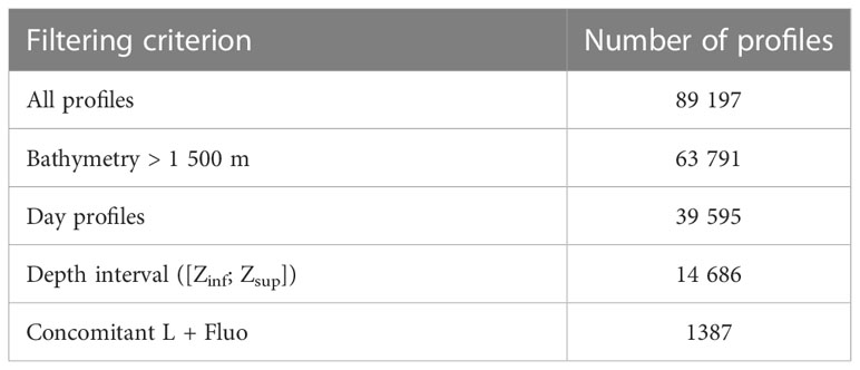
Table 2 Dataset selection criteria and number of selected PAR profiles.

2.2 Data processing

2.2.1 Light profiles and derived quantities

The light sensor embedded in the SRDL is a Hamamatsu S1227-1010BR photodiode (340-1000 nm spectral response range, 100 mm² effective photosensitive area). The photodiode points to the right side of the animal with a 90° angle compared to the frontward axis of the animal. The SRDL light sensor provides an estimate of the diffused light level in the animal’s environment (L, expressed in μmol quanta.m^-2.s^-1). The vertical profiles of light ranged from the maximum diving depth of the animal up to the surface. The processing steps of the raw vertical profiles of light include (for detailed description of the processing steps and graphical support, see supplementary material, Text S1 and Figure S1): detection of the dark depth; dark-offset correction; removal of saturated values at the surface; application of a piecewise cubic polynomial fit. The applied piecewise polynomial fit is constrained, so that L monotonously decreases with depth. The vertical diffuse attenuation coefficient for L (K_L, m^-1) was derived from the processed light profiles. Vertical profiles of K_L were defined with the same vertical resolution as light profiles (i.e. 1 m) and computed as follows:

$\begin{array}{ll}{K}_L(z)=\frac{d}{dz}(log(L(z)))& (1)\end{array}$

where z refers to the depth of the measurement.

The present analysis focuses on daylight periods only. According to the location and time of each profile, the solar angle was computed and only light profiles with positive solar angle (i.e. above the horizon) were retained. Profiles with no location available (23%) were still examined to recover the day/night information from the mean surface values of L. This was enabled by the significant difference observed in the mean surface values of L between day (35 μmol quanta.m^-2.s^-1 +-14) and night (0.65 μmol quanta.m^-2.s^-1 +-3.7). As a result, 39 395 day profiles (62%) were retained after the filtering of the light profiles based on the daylight period criterion (see Table 2).

Following the processing of the raw light profiles, the euphotic depth (Z_eu) and the penetration depth (Z_pd) were computed. Z_eu is defined as the depth at which L is reduced to 1% of its value just below the surface. Z_eu was only computed for light profiles with no sensor saturation in the surface layer. Z_pd (also called first optical depth) characterizes the thickness of the superficial layer of the ocean “seen” by satellites and was defined as Z_eu/4.6 (Gordon and McCluney, 1975; Morel, 1988).

2.2.2 Temperature, salinity and mixed layer depth

SRDLs carry a Conductivity, Temperature and Depth (CTD) sensor head. Temperature (T) and salinity (S) profiles, defined from the maximum diving depth of the animal up to the ocean surface, were quality controlled and corrected to prevent density inversions according to the algorithm proposed in Siegelman et al. (2019b). Density profiles were computed based on temperature and salinity profiles. The mixed layer depth (Z_MLD) was computed using a density threshold of 0.03 kg.m^-3 with respect to a near-surface value at 10 m depth (de Boyer Montégut, 2004).

2.2.3 Fluorescence profiles and derived quantities

SRDLs also include a fluorometer (Valeport Hyperion 470 nm/696 nm emission/reception) that sample Fluo at 0.5 Hz. However, to optimize tags’s energy consumption, their Fluo sampling resolution was reduced so that the onset of the fluorescence sensor was triggered only every ~15 dives and Fluo was only sampled during the ascending phase of the dives from Z_inf = 200 m to the surface. Accordingly, the SRDLs performed around four fluorescence profiles every 24 hours. The processing steps of the raw vertical profiles of Fluo include (for detailed description of the processing steps and graphical support, see supplementary material, Text S2 and Figure S2): dark-offset correction; Non-Photochemical Quenching (NPQ) correction; spikes smoothing with a piecewise cubic polynomial fit. Finally, the smoothed, dark- and NPQ-corrected Fluo data (hereafter denoted [F^Fluo]) were converted into [Chla]. The actual Chla concentration derived from [F^Fluo] ([Chla^Fluo] hereafter), was obtained by applying a calibration coefficient to the [F^Fluo] data. A specific calibration coefficient was computed for each tag, based on both K_L and the comparison of in-situ data with concomitant satellite-based [Chla] observations (see details in Section 2.4).

A series of metrics was computed from the vertical profiles of [Chla^Fluo]. Defined for each profile, the metrics were (see Figure 2):

FIGURE 2

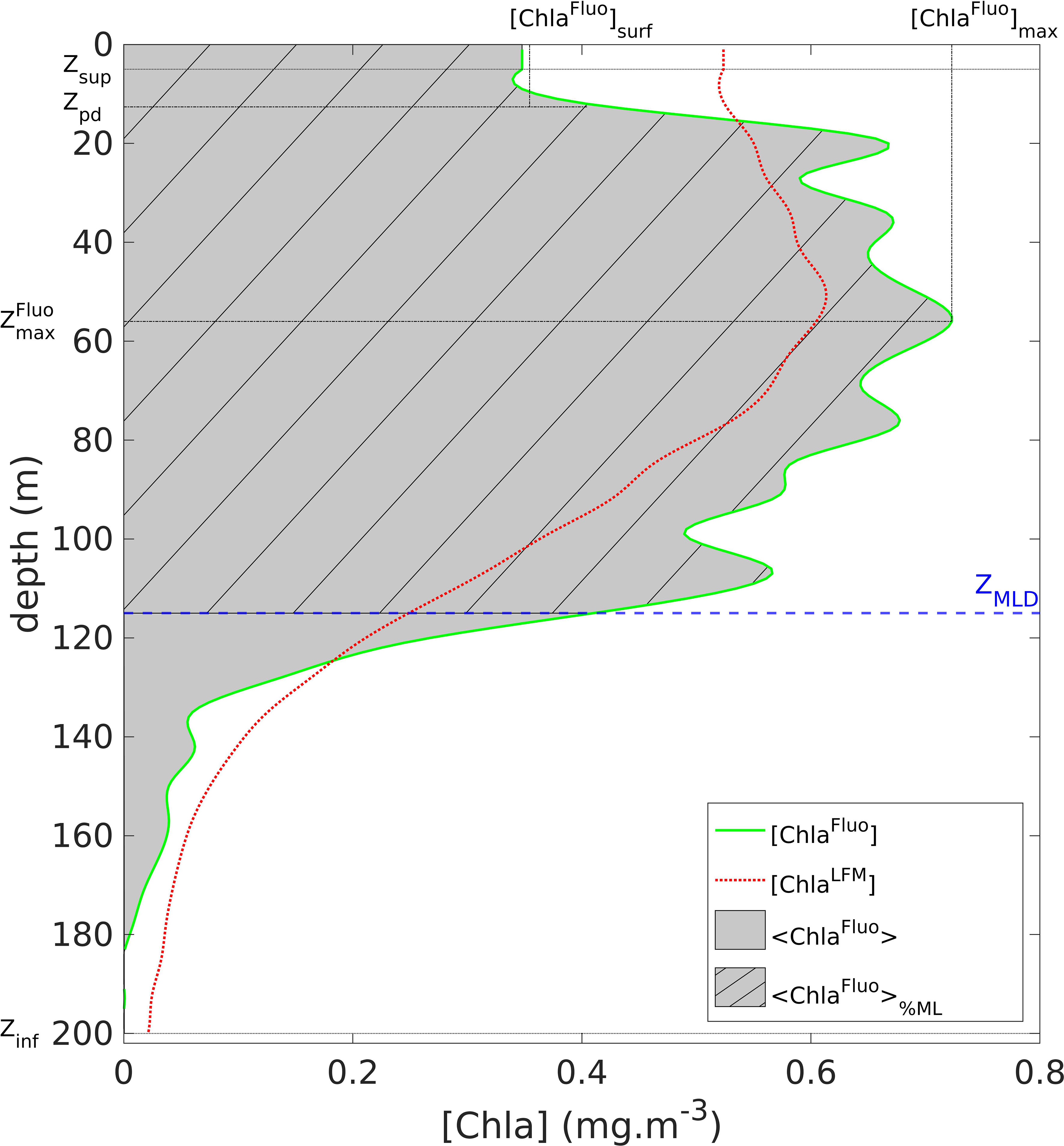
Figure 2 Graphical representation of the metrics defined on a vertical profile of [Chla^Fluo]: <Chla^Fluo>, [Chla^Fluo]_max, $Z_{max}^{Fluo}$, [Chla^Fluo]_surf (see Section 2.2.3). The solid green line represents the [Chla^Fluo] data (for detailed information about the Fluo data processing, see Section 2.2.3 and supplementary material, Text S2 and Figure S2). The gray area represents <Chla^Fluo>, the vertically-integrated amount of Chla. The dashed blue line represents Z_MLD. The dashed area materializes <Chla^Fluo>_%ML, the proportion of <Chla^Fluo> located above Z_MLD. The red dotted line represents the corresponding predicted [Chla^LFM] profile (see Section 2.5). When necessary, the metrics were identically computed on the vertical profiles of [F^Fluo], [F], [F^LFM] and [Chla^LFM].

- <Chla^Fluo>, the water-column integrated value of [Chla^Fluo] defined as

$\begin{array}{ll}\langle Chl{a}^{Fluo}\rangle ={\int }_{Z_{inf}}^0[Chl{a}^{Fluo}](z)dz& (2)\end{array}$

- [Chla^Fluo]_max, the maximum value of [Chla^Fluo]

- $Z_{max}^{Fluo}$, the depth where [Chla^Fluo] (z) = [Chla^Fluo]_max,

- [Chla^Fluo]_surf, the surface value of [Chla^Fluo] defined as

$\begin{array}{ll}{[Chl{a}^{Fluo}]}_{surf}=\overline{{[Chl{a}^{Fluo}]}_{0⩽z⩽Z_{pd}}}& (3)\end{array}$

Additionally, the percentage of Chla within the mixed layer was defined as

$\begin{array}{ll}{\langle Chl{a}^{Fluo}\rangle }_{\%ML}=\frac{100}{\langle Chl{a}^{Fluo}\rangle } {\int }_{Z_{MLD}}^0[Chl{a}^{Fluo}](z)dz& (4)\end{array}$

When relevant, the same metrics were computed for any other variable defined on the vertical in the present study (e.g. [F^Fluo]) with the same notations.

2.3 Linear Functional Model principle

The Linear Functional Model (LFM) developed in the present study is a statistical model based on Functional Data Analysis (Ramsay and Silverman, 1997). The LFM was used as an inference tool to predict [Chla] from K_L. The model is constructed from a statistical sample composed of concomitant vertical profiles of K_L (predictor) and [Chla] (observations), following the method described in Bayle et al. (2015). With the statistical sample at hand, the LFM is designed to minimize the error between model predictions and observations. The functional approach, by handling the vertical profiles as functional variables (i.e. curves), presents the advantage of integrating the shape of the profiles in the analysis (for detailed information about the construction of the model, see Bayle et al., 2015 and supplementary material, Text S4 and Figures S4-S5).

The statistical sample was composed of vertical profiles continuously defined on a depth interval ranging at least from Z_sup = 5 m to Z_inf = 200 m. The predicted profiles were defined on the same depth interval. The main limiting factor for the determination of Z_sup was the recurrent saturation of the light sensor at the surface (39% of the light profiles were saturated down to at least 5 m depth, see Table 2 and supplementary material, Figure S1). The choice of Z_inf was determined by the maximum depth of the Fluo measurements. For a proper interpretation of the results, the values in the upper 0-5 m layer of the predicted profiles were extrapolated from z = Z_sup to the surface with their value at z = Z_sup. [F^Fluo] and [Chla^Fluo] values issued from Fluo measurements in the 0-Z_sup layer, meanwhile, were generally available. Following the filtering of the profiles based on the depth-interval criterion, the dataset contains 14 686 light profiles (from which K_L is derived, see equation 1), which includes 1 387 concomitant L and Fluo (i.e. [F^Fluo] or [Chla^Fluo]) profiles. The number of L profiles following the application of the successive selection criteria is summarized in Table 2.

In the present study, the LFM approach was used to predict either [F^Fluo] or [Chla^Fluo] from K_L, with different objectives, described hereafter (see Sections 2.4 and 2.5).

2.4 Fluo calibration

The calibration procedure applied to the in-situ [F^Fluo] data aims at ensuring (1) the interoperability of the tags through the intercalibration of the Fluo sensors and (2) the consistency of the outputs of the model developed in the present study in terms of absolute values of in-situ [Chla] compared to satellite estimates. This two-step sequence is described hereafter (see flowchart, Figure 1).

Step 1: LFM-based (relative) calibration

The predictive capabilities of the LFM approach were first exploited to intercalibrate the Fluo sensors. The LFM-based intercalibration step consists in predicting [F^Fluo] from K_L with a model that merges observations from all the tags. The predicted variable is hereafter denoted [F^LFM]. Within this step, the focus is not on the reconstruction of vertical profiles of [F^Fluo] but the intended goal is to examine and quantify the relative biases between the Fluo sensors. Consequently, rather than retrieving the parametric definition of the K_L-to-[F^Fluo] functional relationship, the comparison between <F^LFM> (predictions) and <F^Fluo> (observations) enables derivation of a correction factor, proper to each tag, that addresses inter-tag variability, with K_L as a common benchmark. The choice of <F^LFM> (i.e. indirectly, K_L) as the reference variable for Fluo intercalibration is discussed further (see Section 4.1). The [F^Fluo] data of Tag e were re-calibrated with the correction factor ${\Gamma }_e^{LFM}$ so that

$\begin{array}{ll}<\text{F}>={\Gamma }_e^{\mathrm{LFM}}.<F^{\text{Fluo}}>& (5)\end{array}$

where <F> is the re-calibrated <F^Fluo> data and e refers to the tag number (see list of tags by tag number in supplementary material, Table S1).

In practical terms, the coefficient ${\Gamma }_e^{LFM}$ (unitless) is the slope of the linear regression between the values of <F^Fluo> and the corresponding predicted values of <F^LFM> for Tag e. To compute the ${\Gamma }_e^{LFM}$ coefficients, the sample of concomitant [F^Fluo] and K_L observations was merged and randomly split into two subsets: 70% of the profiles were used to construct the LFM (970 profiles). The remaining 30% (417 profiles) were used to evaluate the ${\Gamma }_e^{LFM}$ coefficients. The sample used to evaluate the ${\Gamma }_e^{LFM}$ coefficients was hence independent from the statistical sample used to construct the model. A bootstrap procedure was performed to gain robustness in the determination of the calibration coefficients: the LFM-based calibration was repeated one thousand times with a different random sampling at each iteration. At each iteration, a ${\Gamma }_e^{LFM}$ calibration coefficient was calculated. Finally, the ${\Gamma }_e^{LFM}$ calibration coefficient retained for Tag e corresponds to the median value of the ${\Gamma }_e^{LFM}$ coefficients iteratively calculated for Tag e.

Step 2: Satellite-based (absolute) calibration

In a second phase of the calibration procedure, a single calibration factor ${\Gamma }_{}^{Sat}$ common to all tags was computed. ${\Gamma }_{}^{Sat}$ was based on ocean-color data as a benchmark to convert [F] into [Chla^Fluo]. Surface measurements of in-situ [F] ([F]_surf) of all the tags were merged and compared to the corresponding satellite-derived estimates of surface [Chla] ([Chla^Sat]_surf).

Matchups between satellite and in-situ data were performed following the procedure described in Bailey and Werdell (2006) using normalized satellite remote sensing reflectance (Rrs) daily Level-3 (L3) products from multiple sensors, with a 4 km resolution. The use of more stringent matchup protocols improves the quality of the matchup exercise (Concha et al., 2021), but critically decreases the number of matchups (Haëntjens et al., 2017; Xi et al., 2020; Terrats et al., 2020), especially in the SO where cloud cover is a strong limiting factor. The narrow time window defined in Bailey and Werdell (2006) (+-3 h) was widened to a 24-hour time window (corresponding to the maximum temporal resolution of L3 ocean-color products). Haëntjens et al. (2017) show that expanding the temporal window from +-3 h to a 24-hour window increases the number of matchups, without significantly impacting the quality of the matchups. Accordingly, the matchup protocol used in the present study was based on the averaged data of a 3 x 3 pixel box centered on in-situ measurement with a 1-day time window. Satellite-derived estimates of surface [Chla] were obtained from the Copernicus Marine Service’s GlobColour data archive (http://www.globcolour.info/). The coefficient ${\Gamma }_{}^{Sat}$ was defined as the slope of the linear regression between [F]_surf and [Chla^Sat]_surf. Finally, the satellite-corrected data [Chla^Fluo] was defined as follows

$\begin{array}{ll}[{\text{Chla}}^{\text{Fluo}}]={\Gamma }^{Sat}.[\text{F}]& (6)\end{array}$

2.5 [Chla] prediction

Following the calibration procedure described in the previous section, the LFM approach was applied for inference purposes. A new LFM was designed to infer [Chla^Fluo] from K_L. Being constructed with [Chla^Fluo] profiles, the resulting LFM model hence inherently contains the calibration of the [F^Fluo] data (i.e. ${\Gamma }_e^{LFM}$ and ${\Gamma }_{}^{Sat}$ coefficients). The output variable is denoted [Chla^LFM] (see flowchart, Figure 1). The objective of the prediction phase is to increase the spatial resolution of the [Chla^Fluo] field description with [Chla^LFM]. The prediction is made on the basis of the 14 686 available light profiles (see Table 2). Prior to the retrieval of the [Chla^Fluo] field at (sub)mesoscale, the performance of the LFM was assessed.

Performance assessment

The sample of concomitant [Chla^Fluo] and K_L observations was likewise randomly split into two subsets: 70% of the profiles for the construction of the LFM (970 profiles) and 30% to assess the performance of the LFM (validation sample, 417 profiles). Assessments regarding LFM prediction error and model performance were carried out on the validation sample by comparing the metrics previously defined for [Chla^Fluo] (see Section 2.2.3) with the same metrics derived from the predicted [Chla^LFM] profiles, namely <Chla^LFM>, [Chla^LFM]_surf, [Chla^LFM]_max, and $Z_{max}^{LFM}$.

(Sub)mesoscale prediction

Following the assessment of the model itself via the analysis performed on the validation sample, the LFM was constructed with the entire sample of concomitant [Chla^Fluo] and K_L profiles (1 387 profiles, see Table 2). Subsequently, a prediction exercise was carried out with the 14 686 available K_L profiles (i.e. including K_L profiles which were not associated with any [Chla^Fluo] data). The aim of the prediction exercise is to predict [Chla] at (sub)mesoscale.

2.6 Spectrum analysis

To further assess the improvement brought by the LFM in terms of spatial resolution, the variance spectra of the tags signals were analyzed. For a surface tracer measured with variable V (e.g. <Chla^Fluo>), the variance spectrum is calculated as the Fourier transform of the squared spatial anomaly of V. As a result, the power spectrum for variable V along the trajectory of an equipped animal depicts the energy of the signal as a function of the spatial frequency in the horizontal plane defined by the ocean surface. The variable on the horizontal axis of the computed power spectra is called wave number (m^-1). Increasing wave numbers correspond to smaller spatial scales.

In the present study, the variance spectra of <Chla^Fluo> and <Chla^LFM> were computed for each tag and compared. An additional variable (hereafter denoted dark^KL) was included in the spectrum analysis, defined as the vertical diffuse attenuation coefficient for L, restricted only to the dark signal of L (see Section 2.2.1 and supplementary material, Text S1 and Figure S1). For each profile, dark^KL corresponds to the mean vertical diffuse attenuation coefficient for L (i.e. the derivative of the log-transformed light profile) from the dark depth to the bottom of the dive. While dark^KL contains no useful information for the inference of <Chla>, it was included in the spectrum analysis as a benchmark in terms of spectral behavior. Since dark^KL is computed from dark noise, the corresponding power spectrum theoretically depicts the behavior of pure instrumental noise. The comparison with dark^KL offers a means to determine if the observed tracers (<Chla^Fluo> or <Chla^LFM>) indeed contain useful signals and depict coherent structures, or conversely, behave like noise.

3 Results

3.1 Calibration

Step 1: LFM-based tag intercalibration

The LFM-based tag intercalibration was performed based on the comparison of <F^Fluo> and <F^LFM> for the validation sample. The calibration coefficients were obtained after one thousand iterations of the LFM-based calibration procedure (see Section 2.4). An illustration of one iteration is presented in Figure 3. Graphical examination of the residuals reveals that they are organized and persistent for a given tag, thus confirming the relevance of the intercalibration method. ${\Gamma }_e^{LFM}$ values ranged from 0.29 for Tag 2 to 1.55 for Tag 17 (see complete list of ${\Gamma }_e^{LFM}$ values in supplementary material, Table S2). Small samples have the highest variability because they are not always well represented with the random sampling. Essentially, gaining robustness in the determination of the coefficient is the reason for performing a bootstrap procedure with one thousand iterations of the random sampling. The LFM-based calibration procedure enables computing of the [F] data, which ensures the interoperability of all the tags.

FIGURE 3

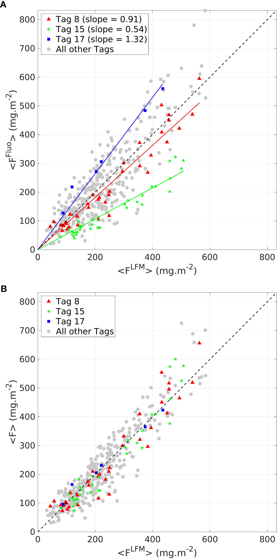
Figure 3 Comparison between <F^Fluo> and <F^LFM > (A) before the LFM-based intercalibration step (B) after the LFM-based intercalibration step. Three tags are highlighted (red triangle, green dots and blue squares, for tags 8, 15 and 17, respectively). Data from all other tags are displayed by gray dots. The black dashed line represents the 1:1 reference line.

Step 2: Satellite-based calibration

The satellite-based calibration procedure was performed after the inter-tag calibration and by merging the [F] data of all the tags. The merging of the tags after the intercalibration step strengthens the power of the satellite-based calibration. Among the 5 791 [F] profiles available, 1 332 successful matchups (23%) were achieved (Figure 4). ${\Gamma }_{}^{Sat}$ = 5.9 was obtained from the slope of the linear regression between [F]_surf and [Chla^Sat]_surf. The regression had a satisfactory significance level (F-test, p-value < 10^-15).

FIGURE 4

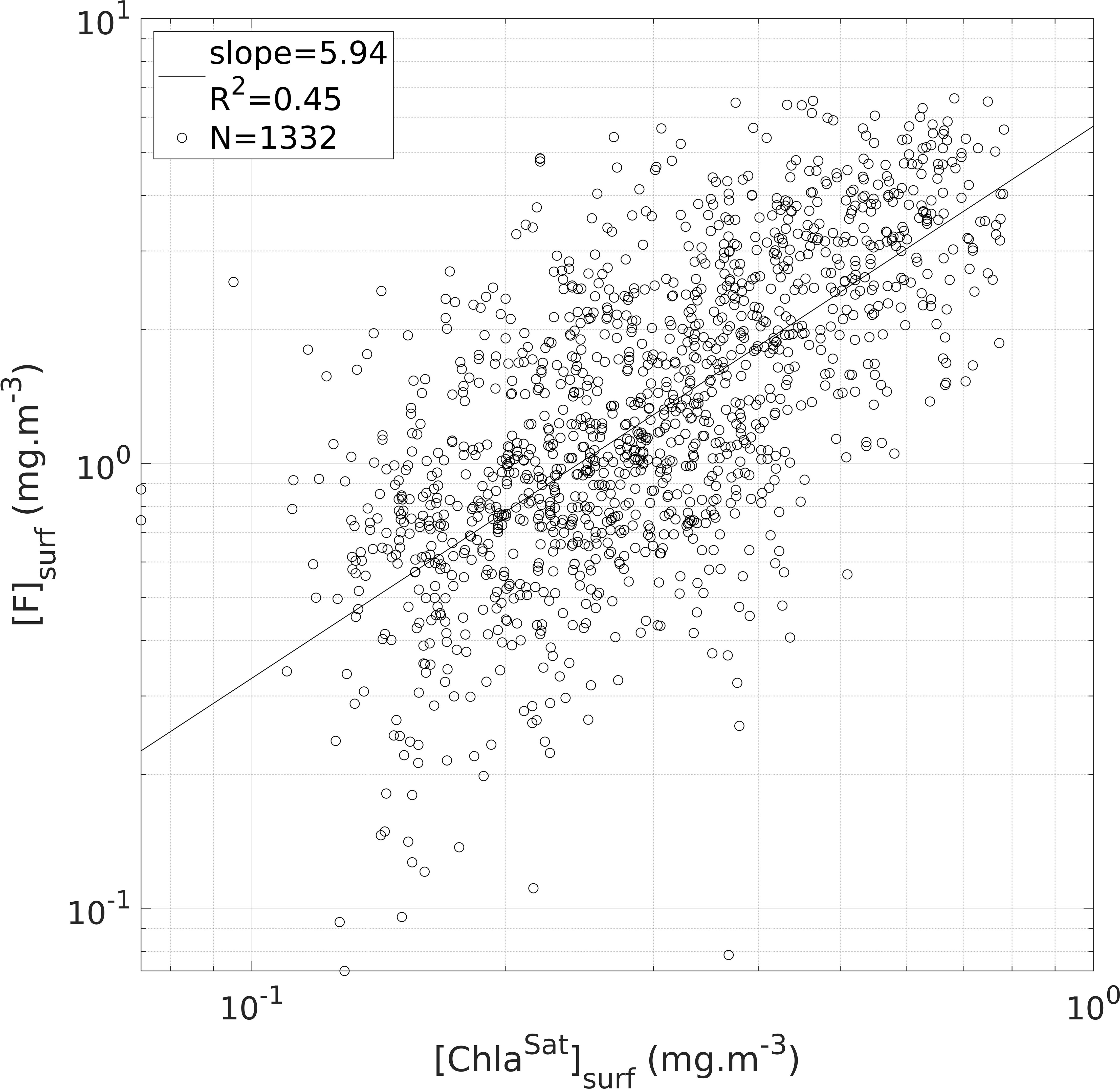
Figure 4 Illustration of the second step of the [F^Fluo] data calibration (see Section 2.4). Estimates of surface [Chla] derived from intercalibrated [F] data ([F]_surf) compared to satellite estimates of surface [Chla] ([Chla^Sat]_surf). The black circles represent the sample points (in total: 1 332 matchups are displayed) and the black line materializes the linear regression of all the sample points (slope = 5.95; R² = 0.45; N = 1 332 matchups).

3.2 LFM assessment

Following the conversion of the homogenized variable [F] into [Chla^Fluo] with the ${\Gamma }_{}^{Sat}$ correction factor (equation 6), a new LFM model was constructed on the basis of concomitant [Chla^Fluo] and K_L profiles, with [Chla^LFM] as the output variable. For assessment purposes, the statistical sample of 1 387 concomitant [Chla^Fluo] and K_L profiles was randomly split (see Section 2.5), so that the LFM was constructed with 70% of the statistical sample and assessed with the remaining 30% (validation sample). The performance of the model was assessed on the validation sample through examination of the metrics defined in Section 2.2.3 (see Figure 2), for both [Chla^Fluo] and [Chla^LFM] (Figures 5A-D).

FIGURE 5

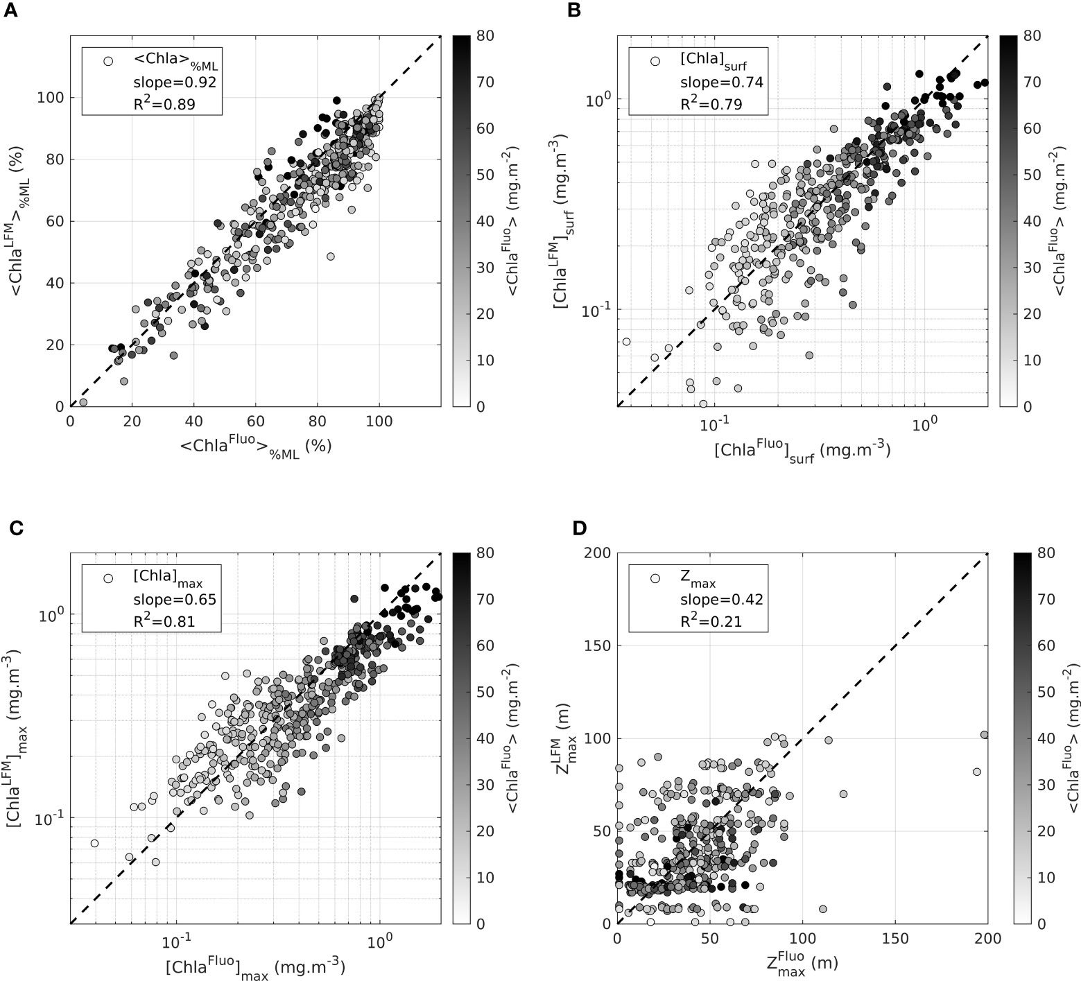
Figure 5 Assessment of the LFM performance on the validation sample. Values in the horizontal axis are metrics derived from the observations ([Chla^fluo]). Values in the vertical axis are metrics derived from the predictions ([Chla^LFM]). The metrics examined to assess the performance of the LFM are (A) [Chla^Fluo]_%ML, the percentage of Chla in the mixed layer (B) the surface value of [Chla], [Chla^Fluo]_surf (C) the maximum value of [Chla], [Chla^Fluo]_max and (D) $Z_{max}^{Fluo}$, the depth of the maximum value of [Chla]. The dashed black lines in each plot represent the 1:1 reference line. The metrics (R², slope) associated with the linear regression performed between model predictions and observations are indicated in each plot.

<Chla>

The predicted <Chla^LFM> differs very little from the targeted <Chla^Fluo> (on average 0.9% +- 21.1). Within a factor ${\Gamma }_{}^{Sat}$, the performance of the model in predicting <Chla^Fluo> both in terms of accuracy and precision is exemplified in Figure 3. The sound agreement between <F^Fluo> and <F^LFM> observed in the intercalibration phase firstly confirms the inference capabilities of the model in terms of accuracy (Figure 3A). Additionally, by correcting the inter-tag variability, the LFM-based calibration procedure (equation 5) inherently increases the precision of the predictions regarding the estimation of the water-column integrated Chla biomass (Figure 3B). Finally, no further change in terms of accuracy and precision is implied by applying the ${\Gamma }_{}^{Sat}$ factor, common to all tags, to obtain [Chla^Fluo] from [F] (equation 6).

<Chla>_%ML

The distribution of the Chla biomass in the vertical is further investigated with the variable <Chla>_%ML. <Chla>_%ML represents the ratio between the Chla content in the 0-Z_MLD layer and the total Chla content in the water column (<Chla>). The slope of the linear regression between <Chla^LFM>_%ML and <Chla^Fluo>_%ML reveals that the model renders, with a satisfactory preciseness, the proportion of the vertically-integrated Chla amount located above and below Z_MLD (slope = 0.92, R² = 0.89). On average, the LFM underestimates <Chla>%_ML by only 4.8% (+-7.2).

[Chla]_surf, [Chla]_max and Z_max

The ability of the model to retrieve the exact vertical distribution of Chla is examined with variables [Chla]_surf, [Chla]_max and Z_max. [Chla^LFM]_surf and [Chla^LFM]_max are compliant with the corresponding observations of [Chla^Fluo]_surf and [Chla^Fluo]_max, although slightly underestimated (Figures 5B,C). The retrieval of Z_max (Figure 5D) is however not satisfying and in some way reveals the limits of the LFM. The poor correlation between $Z_{max}^{Fluo}$ and $Z_{max}^{LFM}$ highlights the weak accuracy of the LFM for retrieving the exact vertical structure of the [Chla] profile.

These results of the model assessment lead to the conclusion that the LFM performs quite well in detecting the amount of Chla in a given profile. The rough vertical distribution of [Chla] in relation to the location of Z_MLD is also well achieved by the model. However metrics on the vertical such as Z_max are not accurately rendered and present high variability.

3.3 Validation with satellite data

Following the assessment of the LFM performance, the model was constructed with all available profiles of [Chla^Fluo] and K_L (1 387 profiles, see Table 2). A prediction exercise was then carried out with all the available K_L profiles (derived from the 14 686 light profiles).

The validity of the LFM predictions was tested through examination of the satellite matchups corresponding to the predicted [Chla^LFM] profiles (see Section 2.4 for the matchup procedure), i.e. by comparing [Chla^LFM]_surf with the co-located [Chla^Sat]_surf estimates. In total, 3 320 successful matchups were achieved (23%). As a direct consequence of the calibration procedure previously performed on the [F^Fluo] data (see Section 3.2), the slope factor of the linear regression of [Chla^LFM]_surf with [Chla^Sat]_surf (slope = 1.01) confirms the consistency of the model outputs in relation to satellite-derived estimates of [Chla] (Figure 6). The compliance of the predicted values with the corresponding [Chla^Sat]_surf estimates validates the LFM predictions. However, a clear divergence is noticeable for low values of [Chla^LFM]_surf ([Chla^LFM]_surf < 0.1 mg.m^-3). To further investigate the validity of the low values of [Chla^LFM]_surf, the available concomitant values of [Chla^Fluo]_surf were examined and compared to [Chla^Sat]_surf (the 14 686 K_L profiles of the prediction exercise include the sample of concomitant [Chla^Fluo] and K_L profiles, i.e. 1 387 [Chla^LFM] profiles with an available concomitant value of [Chla^Fluo]). The comparison of [Chla^Fluo]_surf values with the corresponding [Chla^Sat]_surf estimates (N = 329 successful matchups), also represented in Figure 6, reveals a similar divergence to that observed for [Chla^LFM] below ~ 0.1 mg.m^-3. The difference between low values of [Chla^LFM]_surf and the corresponding [Chla^Sat]_surf estimates is therefore attributable to the discrepancy between in-situ and satellite measurements of [Chla] (discussed further, see Sections 4.2 and 4.3.2) rather than to a model deviation. Low values of [Chla^LFM]_surf are hence valid in the sense that they match with the targeted [Chla^Fluo]_surf.

FIGURE 6

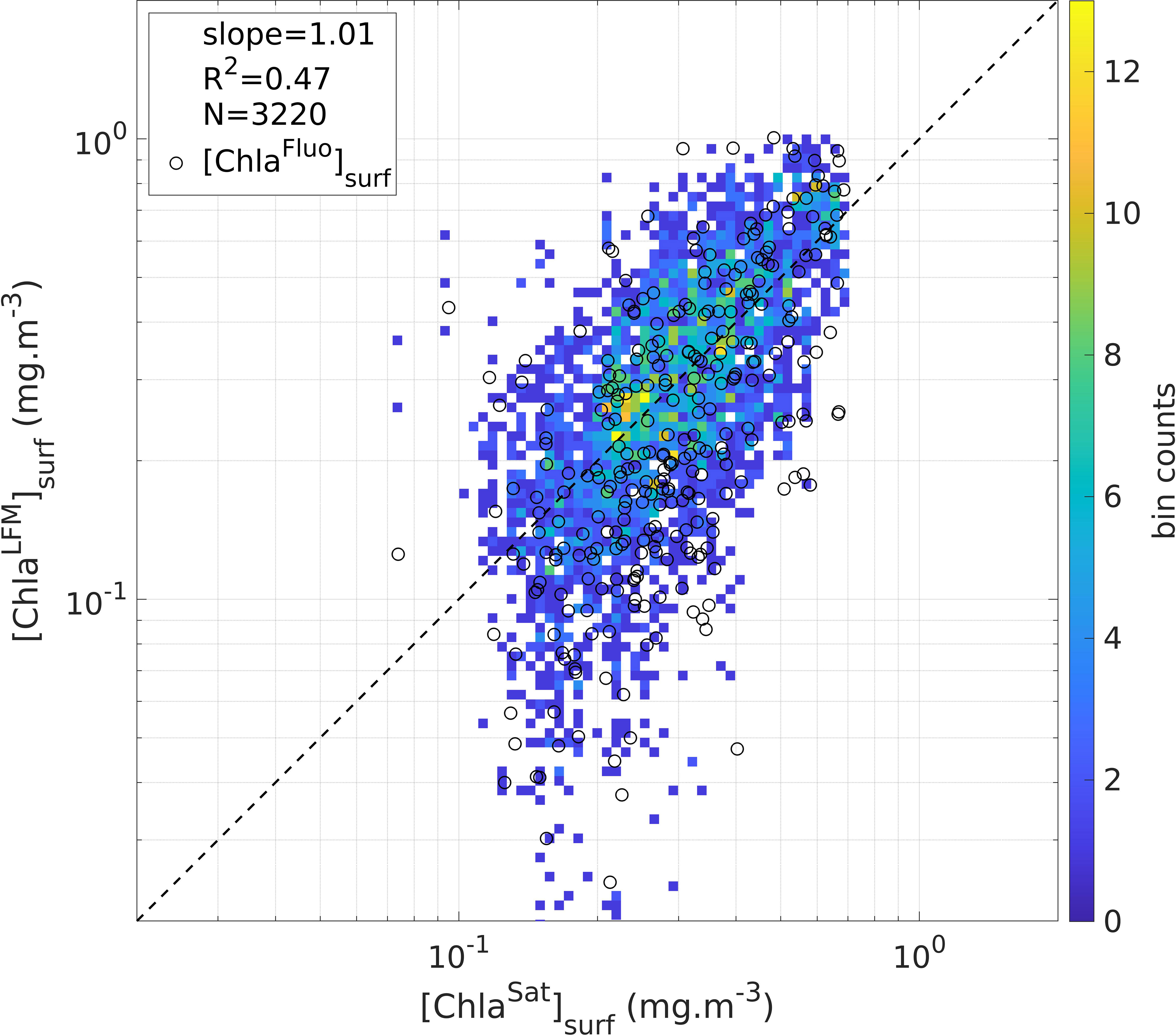
Figure 6 Estimates of surface [Chla] derived from LFM predictions ([Chla^LFM]_surf) compared to satellite estimates of surface [Chla] ([Chla^Sat]_surf). The color of the pixels represent the density of the points in the plot (in total: 3 320 matchups are displayed). The dashed black line materializes the linear regression including all matched samples of [Chla^LFM]_surf and [Chla^Sat]_surf (slope = 1.01; R² = 0.47; N = 3 320 matchups). The black circles represent the available concomitant values of [Chla^Fluo]_surf (N = 329 successful matchups within the 1 387 [Chla^Fluo] profiles used to construct the model, see Section 3.3).

3.4 Application: (sub)mesoscale retrieval

3.4.1 Transect of a SES equipped in Kerguelen

A subset of the SES dataset corresponding to a single individual transect (Tag 3) is shown in Figure 7. The transect is 5 746 km long and covers 70 days at sea, between 25-Oct-2019 and 02-Jan-2020 (Figure 7A). The transect comprises 234 profiles of [Chla^Fluo] and 879 light profiles. One notable detail regarding the transect of Tag 3 is the malfunctioning of the fluorescence sensor during a certain period of the deployment. As a consequence, no Fluo data were available for the time interval extending from 09-Nov-2019 to 02-Dec-2019 (over the same period, 342 T, S and light profiles were sampled by the SRDL).

FIGURE 7

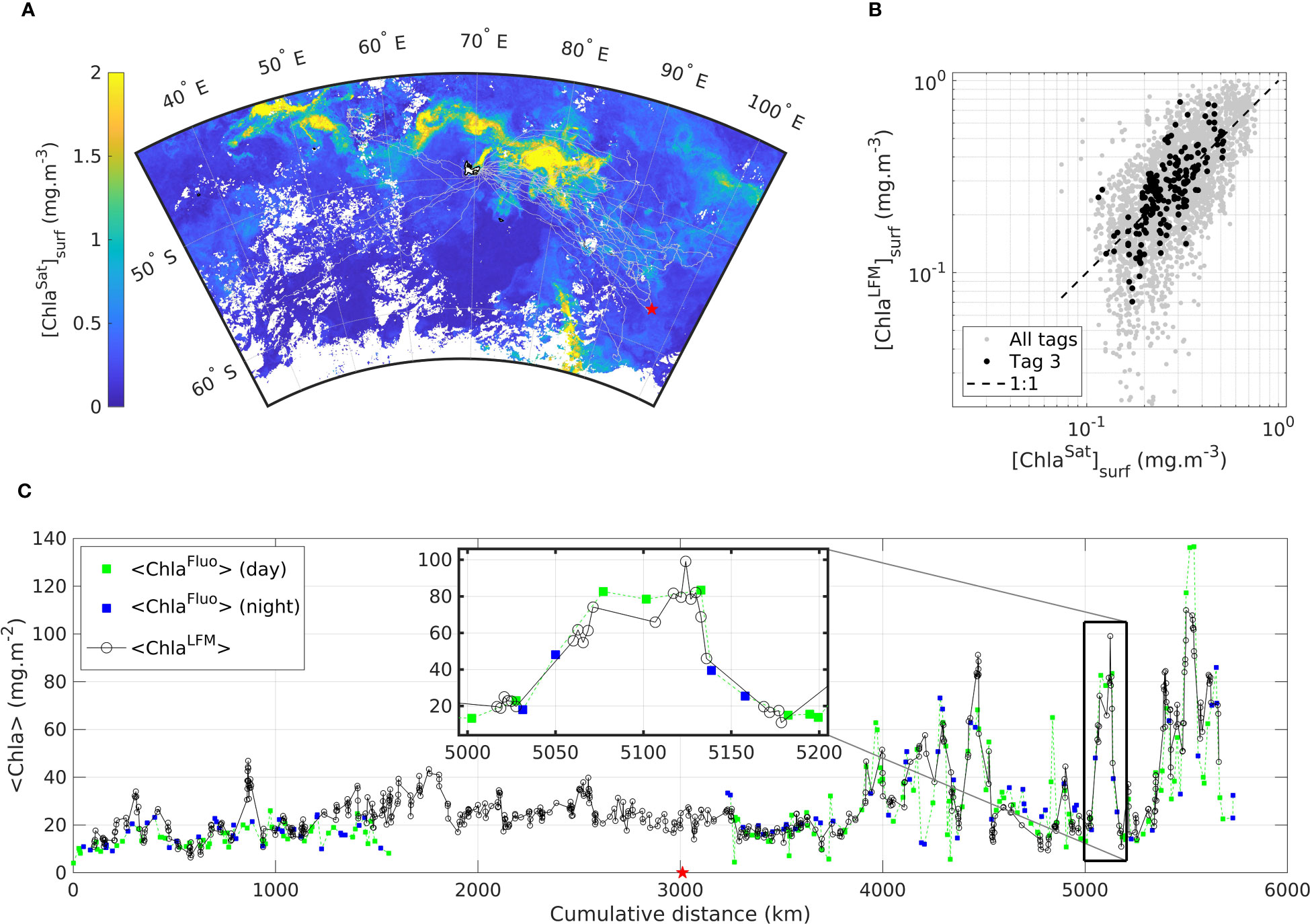
Figure 7 Transect of a SES equipped in Kerguelen in October 2019 with SRDL referred to as Tag 3 including (A) a map of the trajectory described by the SES from 25-Oct-2019 to 02-Jan-2020 departed from- and arrived at Kerguelen (B) comparison of [Chla^LFM]_surf with [Chla^Sat]_surf for Tag 3 and (C) <Chla> as measured (<Chla^Fluo>) and predicted (<Chla^LFM>) along the transect of Tag 3, where green (blue) squares represent the <Chla^Fluo> data measured during the day (night) and black circles represent <Chla^LFM>. The inset in (C) highlights the data on a section of the animal transect (~200 km). The red star in (A) and (C) represents the furthest location from Kerguelen in the trajectory of the animal equipped with Tag 3. Light gray dots in (A) and (B) represent the data of all the other tags included in the present study. The dashed black line in (B) represents the 1:1 reference line. The background map in (A) is the climatology of [Chla^Sat]_surf derived from GlobColour computed for each pixel as the mean value of [Chla^Sat]_surf during the month of November 2019.

The comparison of <Chla^Fluo> and <Chla^LFM> along the animal’s trajectory clearly reveals that the <Chla> signal is well captured by the model. K_L-based LFM predictions faithfully reproduce [Chla^Fluo] observations at water-column level. Additionally, as previously observed when merging all the tags (Figure 6) the general strong correlation between [Chla^Sat]_surf and [Chla^LFM]_surf (Figure 7B) confirms the validity of the LFM predictions. [Chla^LFM] data are especially valuable during the period for which no Fluo data were available due to the malfunctioning of the fluorescence sensor: the missing block (23-days long) of [Chla^Fluo] data was retrieved thanks to the [Chla^LFM] predictions. Inversely, [Chla^Fluo] estimates are available at night when no [Chla^LFM] profiles could be derived from variable L (see inset in Figure 7C). Both situations emphasize the complementary assets of [Chla^Fluo] and [Chla^LFM] estimates. Due to the fact that <Chla^LFM> estimates are available at a higher spatial resolution than that of <Chla^Fluo> (see inset in Figure 7C) during daylight periods, LFM predictions performed between two consecutive [Chla^Fluo] profiles enable the scale of the observations to be refined. The gain relative to the spatial resolution of <Chla^LFM> estimates compared to <Chla^Fluo> is examined hereafter.

3.4.2 Variance spectra

The variance spectra of <Chla^Fluo> and <Chla^LFM> were computed for each tag included in the present study (see Section 2.6). A specific focus was placed on Tag 11 for which the recordings of both Fluo and L were continuous (uninterrupted) during the studied transect. The variance spectrum of dark^KL for Tag 11 was also computed. The highlighted transect corresponding to Tag 11 is 2 231 km long and covers 43 days at sea (between 19-Oct-2018 and 30-Nov-2018). The transect comprises 209 profiles of [Chla^Fluo] and 851 light profiles.

The variance spectra of both observations and predictions of <Chla> along the transect of Tag 11 were compared (Figure 8). The extension of the <Chla^LFM> signal towards the (sub)mesoscale is clearly visible through comparison of the variance spectra of <Chla^Fluo> and <Chla^LFM>. While the smallest spatial scale reached with [Chla^Fluo] observations is ~21 km in the example of Tag 11, the spectrum of the LFM predictions extends to a spatial scale of ~2 km.

FIGURE 8

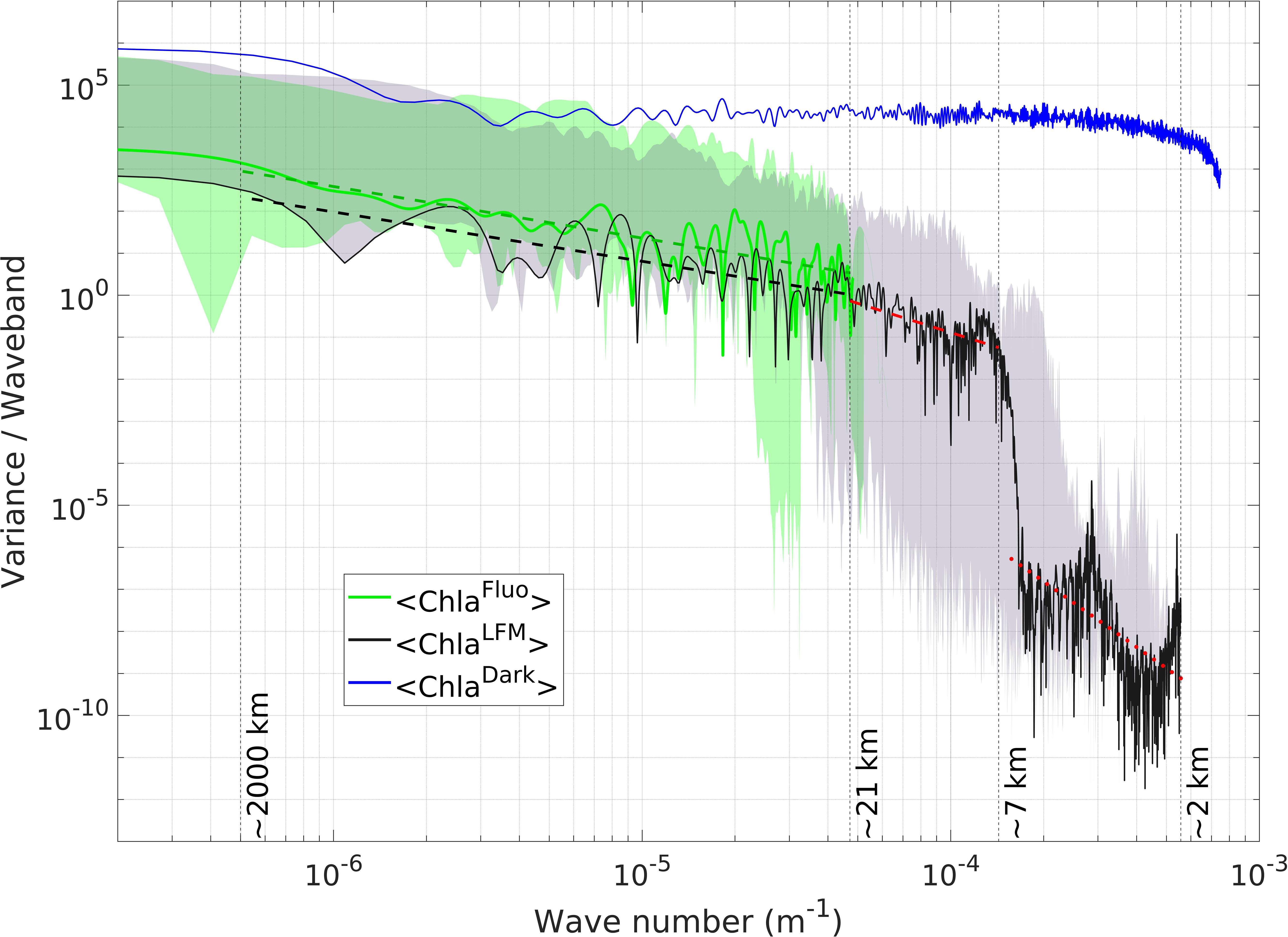
Figure 8 Variance spectrum of <Chla> from observations and model predictions along the trajectory of Tag 11. Increasing wave numbers correspond to smaller spatial scales (see Section 2.6). The green (black) solid line represents the variance per waveband of the <Chla^Fluo> (<Chla^LFM>) signal. The blue solid line represents the variance spectrum of dark^KL. The green (gray) shaded area represents the envelope of the <Chla^Fluo> (<Chla^LFM>) spectra. The envelope encompasses the minimum and the maximum variances per waveband obtained in the dataset of the 18 SES tags included in the present study. The green (black) dashed line represents the linear regression of the variance spectra of <Chla^Fluo> (<Chla^LFM>) on the spatial scale interval between ~2 000 km and ~21 km, with a spectral slope equal to -1.22 (-1.17). The dashed (dotted) red line represents the linear regression of the variance spectrum of <Chla^LFM> on the spatial scale interval between ~21 km and ~7 km (~7 km and ~2 km). The exact corresponding wave numbers are 5 10^-7 m^-1 (~2 000 km), 4.7 10^-5 m^-1 (~21 km), 1.4 10^-4 m^-1 (~7 km) and 5 10^-4 m^-1 (~2 km). (For the determination of the thresholds used for the piecewise linear regressions calculated on the variance spectra of <Chla^Fluo> and <Chla^LFM>, see supplementary material, Text S7 and Figures S8-S9).

On the interval where both signals are defined, a clear energy decay is visible in the variance spectra of <Chla^Fluo> and <Chla^LFM>, following a power-law behavior in k^-a (where k is the wave number, and -a the spectral slope on a log-log plot). For scales larger than ~21 km, the spectral slope of the <Chla^LFM> signal (k^-1.17) is in line with the spectral slope of <Chla^Fluo> (k^-1.22), attesting to the good agreement between observations and model predictions (for interpretation of the spectral slopes, see Section 4.3.4). From ~21 km to ~7 km, the <Chla^LFM> signal similarly follows a power-law behavior with a spectral slope equal to -2.3 (i.e. a steeper decrease than at larger spatial scales). From ~7 km down to ~2 km the spectral slope is -5.2, but this part of the spectrum appears to be much noisier.

The spectrum of dark^KL derived from the dark noise of L, computed for Tag 11 (see Section 2.6), was added in Figure 8 to illustrate the spectral characteristics of dark noise. The variance spectrum of dark^KL is almost flat for wave numbers smaller than ~3 10^-4 m^-1, meaning that all spatial frequencies larger than ~3 km are equally represented within the dark^KL signal. Such a spectrum is coherent with the definition of pure noise and contrasts with the power-law behavior of <Chla^Fluo> and <Chla^LFM>.

For spatial scales smaller than ~21 km, where only <Chla^LFM> is defined, two distinct wave number intervals are clearly discernible, separated by a pronounced drop in the energy of the signal, located at around ~7 km in the case of Tag 11. The signal gets much noisier after the energy drop. A similar behavior was observed for every tag included in the present study, namely a pronounced energy drop materializing a spatial scale threshold below which the spectrum follows a power-law behavior, and above which the signal loses coherency (i.e. gets much noisier). It is consequently reasonable to consider that the interpretations of the structures depicted by the <Chla^LFM> signal are valid up to the scale of the energy-drop threshold and should be discarded for higher spatial frequencies. In the case of Tag 11 (specifically highlighted in Figure 8), the spatial resolution of the observations hence extends from ~21 km with Fluo to at least ~7 km with LFM predictions. The energy-drop threshold was different for each tag. The shaded gray area in Figure 8 represents the envelope of the <Chla^LFM> spectra, encompassing the minimum and the maximum variances per waveband obtained in the dataset of the 18 SES tags included in the present study. The envelope of the <Chla^LFM> spectra reveals that the spatial scale of the energy drop spreads from ~30 km to ~4 km (corresponding to wave numbers of ~3 10^-5 m^-1 and ~2.5 10^-4 m^-1, respectively).

Similarly, a comparable energy drop was observed in the <Chla^Fluo> spectrum for some, though not all, of the tags included in the present study (see green shaded area in Figure 8). The energy drop in the <Chla^Fluo> spectra occurred at larger spatial scales than in the <Chla^LFM> spectra, starting from ~45 km.

4 Discussion

4.1 Exploiting light-Fluo synergies through LFM: Data intercalibration and homogenization

Including data from multiple tags in a study raises the issue of the intercalibration of the fluorescence sensors, a critical point when [Chla] estimates are to be derived from Fluo measurements. Evidences of inter-sensor variability have already been pointed out for different fluorometer models (e.g. Guinet et al., 2013; Xing et al., 2014; Keates et al., 2020), emphasizing the necessity of homogenizing the Fluo data from one tag to another before any further analysis. A common benchmark which provides an absolute Fluo to [Chla] conversion theoretically resolves the inter-tag calibration issue. However, the fluorescence sensors embedded in the tags examined in the present study did not undergo any in-situ calibration process and not all of them could be successfully independently calibrated with concomitant satellite estimates of [Chla] (see Section 4.2).

The lack of any direct comparative benchmark for Fluo led to an investigation of the in-situ data concomitantly sampled by the SRDLs in order to best take advantage of them. Accordingly, the first step of the Fluo calibration procedure relies on variable K_L as a common variable to all the tags and exploits the predictive assets of the LFM to intercalibrate the Fluo sensors. It has been previously demonstrated (Morel, 1988; Morel and Maritorena, 2001) that the optical properties of open-ocean waters (so-called case 1 waters) are essentially driven by their phytoplankton content (depicted by the concentration in Chla) and their associated living or inanimate materials (heterotrophic organisms, including bacteria; various debris; and excreted organic matter). Such relationships between the water-column algal content and optical properties have also been used to deeper examine the data acquired by electronic tags deployed on pelagic animals (Teo et al., 2009; Jaud et al., 2012; Bayle et al., 2015). Here, we further exploit the synergy between K_L and Fluo by proposing a method to make the Fluo data from different (and not intercalibrated) tags inter-comparable. As K_L depicts gradients (derivative) of light in the water column rather than absolute light levels, it is much less dependent on the light sensor design, calibration or drift (e.g. biofouling). Therefore, K_L is a highly robust measurement that can potentially serve as a reference measurement for long-term observations like those obtained via autonomous platforms (floats, gliders) or animals.

In this context, a method based on an analytical relationship linking the diffuse attenuation for downward irradiance K_d to [Chla] (Morel and Maritorena, 2001) was first proposed in Xing et al. (2011) to take advantage of fluoresence profiles acquired by BGC-Argo floats simultaneously with radiometric profiles of downward irradiance. The relationship between [Chla] and downward irradiance is investigated at three specific wavelengths and enables the calibration of Fluo data in terms of [Chla] as well as the handling of any potential drift of the Fluo sensor over time. In our study, the SRDL provides a measurement on a large spectral interval (340 to 1000 nm, see Section 2.2.1). Additionally the quality of the radiometric measurements performed with the SRDL is not comparable to those of BGC-Argo floats, for which the verticality of the sensor as well at the exact time of the sampling are monitored to optimize the quality of the radiometry data (see Xing et al., 2011; Organelli et al., 2016). As a consequence, we judged relevant to adopt a less strictly analytical method for the matching between K_L and [Chla] but instead, encompass the variability in the entire visible spectrum with a shape-based approach (LFM). The LFM imposes no a priori model regarding the relationship between K_L and [Chla] during the construction of the model, leaving the calibration of Fluo in terms of [Chla] for a later stage of the procedure. Accordingly, the first step of the Fluo calibration procedure solely relies on variable K_L as a common variable to all the tags and exploits the predictive assets of the LFM to intercalibrate the Fluo sensors.

Finally, it is worth noting that the power and robustness of the LFM depend on the size of the statistical sample used to construct the model (for results regarding the robustness of the model in relation to the composition of the statistical sample used to construct the model, see supplementary material, Text S5 and Figure S6). The amount of data available to feed the model is limited by the fact that K_L is only exploitable during daytime (in the present study, only light profiles associated with a positive solar angle were selected). During daytime, the determination of K_L is partially influenced by the solar angle (Morel et al., 2007). Nevertheless, the model’s accuracy appears not to be influenced by solar angle as the prediction error presented a similar dispersion for all positive values of the solar angle (see supplementary material, Text S6 and Figure S7).

4.2 Matching in-situ and satellite measurements for absolute calibration

A per-tag satellite-based calibration procedure comparing surface measurements of Fluo with concomitant satellite estimates of [Chla] is an alternative way to convert [F^Fluo] into actual [Chla] (e.g. Lavigne et al., 2012; Terrats et al., 2020), in particular when no pre-deployment HPLC [Chla] data are available for the calibration of the tags. However, although surface Fluo measurements could be quite successfully matched with satellite data for some of the tags, others critically lacked sufficient satellite coverage to permit trustworthy calibration. The per-tag satellite matchup procedure hence could not be generalized to all the tags. Therefore the LFM-based step discussed above was an essential requirement to correct for inter-tag variability and to render all the [F^Fluo] data interoperable, thus constituting a homogeneous data base from which absolute calibration (i.e. conversion from [F] into [Chla], see flowchart, Figure 1) could subsequently be established. The merging of all the intercalibrated tags indeed reinforces the quality of the comparison with satellite data and increases the robustness of the calibration procedure.

The second step of the Fluo calibration therefore converts the fluorescence signal into an estimate of [Chla], based on concomitant satellite measurements. Satellite-based ocean-color algorithms for the retrieval of [Chla] do not perform equally in all regions of the globe (Szeto et al., 2011). Specifically for the SO, the need for having regionally-tuned algorithms is a matter of debate, with some arguing that satellite-derived [Chla] is underestimated by a 2-3 factor (Guinet et al., 2013; Johnson et al., 2013), while others reporting that standard algorithms for the global ocean perform well (Haëntjens et al., 2017). The standard satellite [Chla] product used here (namely, the Copernicus Marine Service’s GlobColour ocean-color data) is a global scale product which we consider to be adapted in the context of the main study purposes. Furthermore, merging all the tags’ data prior to the satellite calibration was relevant because all the tags were deployed in the same region, namely the Kerguelen Islands, which reinforces the interoperable nature of the various tag observations.

4.3 Assessment of the method

4.3.1 Retrieval of the vertical distribution of Chla

Following the constitution of calibrated [Chla] datasets, the LFM was developed such that the modeled [Chla^LFM] matched as closely as possible the targeted [Chla^Fluo]. The retrieval of <Chla^Fluo> was generally well achieved with the LFM predictions (see Section 3.2). The model however lacks accuracy along the vertical dimension. In the SO, Z_MLD is a major driver in the vertical distribution of Chla. For a large majority of profiles, the mixed layer contains most of the Chla biomass and [Chla] is homogeneous within this layer (Cornec et al., 2021). Yet a remainder of the vertically-integrated Chla can be present below Z_MLD. Since the model also proved to successfully estimate <Chla^LFM>_%ML (Figure 5A), an estimate of this remainder is achievable. Here, we make the hypothesis that this remainder may not be present deeper than 1.5 times Z_eu. As a consequence, by associating <Chla^LFM> predictions with <Chla^LFM>_%ML, Z_MLD and Z_eu, an insight into the distribution of Chla in the vertical is still achievable even in the absence of properly reconstructed vertical profiles.

4.3.2 Fluo uncertainty

The LFM is based on estimates derived from fluorescence measurements, with the aim of reproducing them. Nevertheless, uncertainties exist regarding the algal biomass estimates derived from fluorescence measurements. The relationship between Chla fluorescence and actual Chla concentration is in particular governed by the fluorescence quantum yield (expressed as: mole emitted photons (mole of absorbed photons)^-1) which depends on many factors, including phytoplankton community composition, photo-physiological as well as nutrient status (Roesler et al., 2017; Schallenberg et al., 2022). The tags included in the present study were all deployed from the Kerguelen Islands, but the trajectories of the equipped animals spread in the ocean from East to West of the Kerguelen Plateau. The Kerguelen plateau region is highly contrasted between the iron-limited western part and the iron-fertilized eastward zone (Blain et al., 2008). The merging of [F^Fluo] data of all the tags as part of the Fluo calibration procedure could thus be in some ways questionable. However, the intercalibration coefficients derived from the LFM predictions were examined and no significant difference was observed between East and West of the Kerguelen Plateau (Mann-Whitney-Wilcoxon test, p-value of 0.63).

4.3.3 Model - observation discrepancies

The LFM is based on the assumption that the presence of phytoplankton is the main source of light attenuation in the water column, as commonly hypothesized when studying oceanic case 1 waters. Accordingly, a minimum bathymetry criterion was fixed to avoid dealing with coastal waters (depth > 1 500 m). However, persistent overestimates of the Chla content are observed in some short portions of the predicted signal (Figure 7C). Such deviations are of special interest for analyzing specific issues or limitations regarding the LFM. Generally however, locally persistent deviations may result from small-scale variations in the bio-optical properties of the corresponding water masses. These could be due the presence of other covarying substances contributing to light attenuation and/or affecting the fluorescence signal (Bricaud et al., 1998; Loisel et al., 2002; Bellacicco et al., 2019). Such small-scale variations were however not investigated in the present study.

4.3.4 Towards filling [Chla] observational gaps at the (sub)mesoscale

One of the potentially interesting outcomes of the development of the present method is that it becomes obvious that measurements of light rather than fluorescence represent a cost-effective alternative for filling [Chla] observational gaps. The observation gap originates from the limitations relative to the power consumption of SRDLs mounted on SESs, which impedes Fluo sampling at a scale compatible with (sub)mesoscale observations. By contrast, measurements of light require less energy and can be performed at much higher spatio-temporal resolution. Comparing the variance spectra of both observations and predictions (Figure 8) corroborates the gain brought by the LFM in terms of spatial resolution. The gain in terms of spatial resolution is also visible on the transect presented in Figure 7C. In the case of the SRDLs, <Chla^LFM> is the only variable defined at (sub)mesoscale and higher to describe phytoplankton dynamics, opening up a new way to fill the (sub)mesoscale observational gap.

The analysis of the variance spectrum of <Chla^LFM> was further used as a means to validate the consistency of the predictions at different spatial scales. At spatial scales where both the measured (<Chla^Fluo>) and the predicted (<Chla^LFM>) signals were available (e.g. from ~2 000 km to ~21 km in the case of Tag 11), the predictions were validated by the similarity between the spectral slopes of <Chla^Fluo> and <Chla^LFM> (Section 3.4.2). At spatial scales where <Chla^Fluo> was not defined (e.g. smaller than ~21 km in the case of Tag 11), the variance spectra of dark^KL and <Chla^LFM> resulted in clearly distinct shapes (Figure 8), hence ensuring that <Chla^LFM> predictions did not result from pure observational noise.

The predicted signal therefore constitutes a useful signal with a coherent energy decrease across the observed spatial scales. From large-scale (~2 000 km) to (sub)mesoscale (O(10-100 km)), the energy decay of the spatial variance observing a power-law behavior in k^-a (for the definition of wave number k and spectral slope -a, see Section 3.4.2) is consistent with the expected behavior of a tracer such as [Chla] (Bracco et al., 2009; Lévy et al., 2018). Furthermore, spectral slopes become more negative as the wave number increases (i.e. the spectrum has a steeper decrease at smaller spatial scales), from ~k^-1 at mesoscale to ~k^-2 at submesoscale (see Section 3.4.2). These slopes are highly consistent with the expected decay slopes of a signal depicting phytoplankton distribution at (sub)mesoscale (Martin and Srokosz, 2002; Callies and Ferrari, 2013; van Gennip et al., 2016).

The energy-drop threshold materializing the validity domain of the predictions (see Section 3.4.2) corresponded for each tag to twice the mean spatial frequency of the tags’ light measurements (for detailed theoretical interpretation of the validity domain, see supplementary material, Text S7 and Figures S8-S9). The energy-drop threshold is hence directly dependent on the inherent properties of the corresponding transect. In the dataset of the 18 SES tags included in the present study, the mean distance between two valid consecutive Fluo profiles is 14.9 km +- 4.1, whereas for light profiles this distance is reduced to 5.9 km +- 3.1. As a result, while on average the SRDL Fluo measurements enable observation of phytoplankton dynamics at spatial scales up to ~30 km, LFM predictions extend the spatial scale of the observations up to ~12 km. In the present study, the gain enabled by the use of <Chla^LFM> as a proxy for <Chla^Fluo> is on average a factor 2.8 +- 0.9 towards finer observation scales.

Although light measurements are obviously restricted to the daytime period it is worth noting that in high-latitude environments with extended day lengths during the productive season, light measurements provided by SES tags might represent a unique tool to better address (sub)mesoscale coupling between physical forcing and biological response. However, independently of the bio-physical processes occurring along the transect of the tag, the spatial resolution of the light measurements performed by the tag directly depends on the horizontal speed of the SES (i.e. the distance between the consecutive dives of the SES, see previous paragraph), and also quite frequently, on the quality and validity of the measurements. For example, in the present study, the saturation issue (see Section 2.2.1 and supplementary material, Figure S1) clearly lowers the spatial resolution achieved by the light measurements. Therefore, our recommendation regarding SRDLs is to implement a less sensitive light sensor to limit sensor saturation under high light levels (mainly occurring around noon, in the surface layer). Theoretically, if the light sensor is free from the saturation issue and all daylight profiles can hence be included in the LFM, the gain in terms of spatial resolution could potentially reach a factor 9, meaning that the method developed in the present study would enable observation of phytoplankton dynamics at a scale of ~3-4 km.

5 Conclusion and perspectives

The present study highlights the benefits of using the LFM both to homogenize the Fluo data from different sensors and to infer the Chla content in the water column. The interest of a model such as the LFM using K_L to describe the dynamics of Chla along the trajectory of an equipped SES stands out especially for a device with severe power consumption constraints such as the SRDL. The substantially low mean error associated with LFM predictions (see Section 3.2) emphasizes the accuracy of the LFM-based method for retrieving the variability of the <Chla> field and extending the spatio-temporal scale of observations (see Section 4.3.4). While the sole use of fluorescence measurements might not be sufficient to access (sub)mesoscale processes, the finer horizontal resolution achievable with LFM predictions unlocks the (sub)mesoscale observation gap of SRDLs.

Examples of SES foraging behavior being influenced by the environmental oceanographic conditions at (sub)mesoscale have already been described (Campagna et al., 2006; Della Penna et al., 2015; Siegelman et al., 2019a). In parallel, while recent missions like SWOT aim at describing the ocean surface dynamics at an unprecedented resolution (15-30 km, see Morrow et al., 2019), the use of <Chla^LFM> as a proxy for <Chla^Fluo> enables the resolution of in-situ biological tracers to be aligned with the spatial scales targeted in such recent missions. Because primary production is largely driven by ephemeral physical processes occurring from the mesoscale (O(100 km)) to the submesoscale (O(10 km)), in-situ information at such scales is critical to describe phytoplankton dynamics (Mahadevan, 2016; McGillicuddy, 2016; Lévy et al., 2018). The improvements brought by the LFM in terms of spatial scales hence contribute key elements for deepening study of the coupling between phytoplankton distribution and the ocean’s physical structure at (sub)mesoscale (including Lagrangian studies, Lehahn et al., 2018), and also provide novel data for studying SES behavior and the horizontal exploration of the ocean by such marine predators.

In this way, the dynamics of phytoplankton along the trajectories of SESs are optimally described by merging satellite-calibrated [Chla^Fluo] data derived from the tags’ fluorescence measurements (covering both day and night periods) with [Chla^LFM] estimates (only available during daylight hours), which improves the spatio-temporal resolution of the data. In the present study, the data from tag deployment campaigns performed between 2018 and 2020 were included. The predictive capabilities of the LFM can possibly be extended towards a larger range of tags, e.g. tags deployed in the past measuring light but not Fluo. Indeed, bio-logging data have proved to be a considerable source of in-situ data at (sub)mesoscale in the SO in the past two decades. Every light profile, despite not providing truly reliable metrics on the vertical, is useful, under the method developed in the present study, to feed biogeochemical models with an estimate of the vertically-integrated Chla amount and the proportion of the Chla amount present within the mixed layer. Datasets comprising hundreds of thousands of in-situ vertical profiles sampled by equipped animals in the SO hence constitute a possible insight into the ocean subsurface to extend the quasi-synoptic - but surface-only - vision provided by satellite data. These numerous profiles are potentially highly valuable data for developing our knowledge about [Chla] variability at different spatio-temporal scales in the under-sampled SO, from short-lived processes to decadal variability.

Data availability statement

Publicly available datasets were analyzed in this study. This data can be found here: The marine mammal data were collected as part of the Système National d’Observation Mammifères Echantillonneurs du Milieu Océanique (SNO-MEMO) and made freely available by the International MEOP Consortium and the national programs that contribute to it. The MEOP data are available at www.meop.net/database/meop-databases. The computer codes produced for the present study are available at https://doi.org/10.17882/93268. The GlobColor products were produced and distributed by the Copernicus Marine Service with support from CNES and ACRI-ST, and are available at http://marine.copernicus.eu/services-portfolio/access-to-products/.

Ethics statement

The animal study was reviewed and approved by the ethics committee “Comité d’éthique Anses/ENVA/UPEC (N° 19-040 #21375)” and the Comité Pour l’Environnement Polaire des Terres Australes et Antarctiques Françaises.

Author contributions

Conceived and designed the study, LLS, HC, and CG; BP helped with the processing of the MEOP data. LLS and DN conceived the functional model and analyzed the model performance. LLS, HC, Fd’O, and CG wrote the manuscript. HC, Fd’O, and CG helped with analyzing the results. LLS, HC, Fd’O, DN, BP, and CG reviewed the manuscript. All authors contributed to the article and approved the submitted version.

Funding

This work was partly funded by the CNES and REFINE (European Research Council, Grant agreement 834177) project. LLS is supported by a joint CNES-CNRS doctoral grant. The elephant seal work was supported as part of the SNO-MEMO and by the CNES-TOSCA project Elephant seals as Oceanographic Samplers of submesoscale features led by C. Guinet with support of the French Polar Institute (programmes 109 and 1201). This research was carried out, in part, at the Centre d’Études Biologiques de Chizé, under a contract with the Centre National d’Études Spatiales (CNES) and at the Laboratoire d’Océanographie de Villefranche.

Conflict of interest

The authors declare that the research was conducted in the absence of any commercial or financial relationships that could be construed as a potential conflict of interest.

Publisher’s note

All claims expressed in this article are solely those of the authors and do not necessarily represent those of their affiliated organizations, or those of the publisher, the editors and the reviewers. Any product that may be evaluated in this article, or claim that may be made by its manufacturer, is not guaranteed or endorsed by the publisher.

Supplementary material

The Supplementary Material for this article can be found online at: https://www.frontiersin.org/articles/10.3389/fmars.2023.1122822/full#supplementary-material

References

Ardyna M., Claustre H., Sallée J.-B., D’Ovidio F., Gentili B., van Dijken G., et al. (2017). Delineating environmental control of phytoplankton biomass and phenology in the southern ocean: Phytoplankton dynamics in the SO. Geophys. Res. Lett. 44, 5016–5024. doi: 10.1002/2016GL072428

CrossRef Full Text | Google Scholar

Bachman S. D., Taylor J. R., Adams K. A., Hosegood P. J. (2017). Mesoscale and submesoscale effects on mixed layer depth in the southern ocean. J. Phys. Oceanogr 47, 2173–2188. doi: 10.1175/JPO-D-17-0034.1

CrossRef Full Text | Google Scholar

Bailey S. W., Werdell P. J. (2006). A multi-sensor approach for the on-orbit validation of ocean color satellite data products. Remote Sens. Environ. 102, 12–23. doi: 10.1016/j.rse.2006.01.015

CrossRef Full Text | Google Scholar

Baldry K., Strutton P. G., Hill N. A., Boyd P. W. (2020). Subsurface chlorophyll-a maxima in the southern ocean. Front. Mar. Sci. 7. doi: 10.3389/fmars.2020.00671

CrossRef Full Text | Google Scholar

Bayle S., Monestiez P., Guinet C., Nerini D. (2015). Moving toward finer scales in oceanography: Predictive linear functional model of chlorophyll a profile from light data. Prog. Oceanogr 134, 221–231. doi: 10.1016/j.pocean.2015.02.001

CrossRef Full Text | Google Scholar

Bellacicco M., Cornec M., Organelli E., Brewin R. J. W., Neukermans G., Volpe G., et al. (2019). Global variability of optical backscattering by non-algal particles from a biogeochemical-argo data set. Geophys. Res. Lett. 46, 9767–9776. doi: 10.1029/2019GL084078

CrossRef Full Text | Google Scholar

Blain S., Quéguiner B., Trull T. (2008). The natural iron fertilization experiment KEOPS (KErguelen ocean and plateau compared study): An overview. Deep Sea Res. Part II: Topical Stud. Oceanogr 55, 559–565. doi: 10.1016/j.dsr2.2008.01.002

CrossRef Full Text | Google Scholar

Blain S., Renaut S., Xing X., Claustre H., Guinet C. (2013). Instrumented elephant seals reveal the seasonality in chlorophyll and light-mixing regime in the iron-fertilized southern ocean: CHLOROPHYLL AND LIGHT IN SOUTHERN OCEAN. Geophys. Res. Lett. 40, 6368–6372. doi: 10.1002/2013GL058065

CrossRef Full Text | Google Scholar

Boehme L., Lovell P., Biuw M., Roquet F., Nicholson J., Thorpe S. E., et al. (2009). Technical note: Animal-borne CTD-satellite relay data loggers for real-time oceanographic data collection. Ocean Sci. 5, 685–695. doi: 10.5194/os-5-685-2009

CrossRef Full Text | Google Scholar

Boyd P. W., Claustre H., Levy M., Siegel D. A., Weber T. (2019). Multi-faceted particle pumps drive carbon sequestration in the ocean. Nature 568, 327–335. doi: 10.1038/s41586-019-1098-2

PubMed Abstract | CrossRef Full Text | Google Scholar

Bracco A., Clayton S., Pasquero C. (2009). Horizontal advection, diffusion, and plankton spectra at the sea surface. J. Geophys. Res. 114, C02001. doi: 10.1029/2007JC004671

CrossRef Full Text | Google Scholar

Bricaud A., Morel A., Babin M., Allali K., Claustre H. (1998). Variations of light absorption by suspended particles with chlorophyll a concentration in oceanic (case 1) waters: Analysis and implications for bio-optical models. J. Geophys. Res. 103, 31033–31044. doi: 10.1029/98JC02712

CrossRef Full Text | Google Scholar

Bushinsky S. M., Landschützer P., Rödenbeck C., Gray A. R., Baker D., Mazloff M. R., et al. (2019). Reassessing southern ocean air-Sea CO 2 flux estimates with the addition of biogeochemical float observations. Global Biogeochem Cycles 33, 1370–1388. doi: 10.1029/2019GB006176

PubMed Abstract | CrossRef Full Text | Google Scholar

Callies J., Ferrari R. (2013). Interpreting energy and tracer spectra of upper-ocean turbulence in the submesoscale range (1–200 km). J. Phys. Oceanogr 43, 2456–2474. doi: 10.1175/JPO-D-13-063.1

CrossRef Full Text | Google Scholar

Campagna C., Piola A. R., Rosa Marin M., Lewis M., Fernández T. (2006). Southern elephant seal trajectories, fronts and eddies in the Brazil/Malvinas confluence. Deep Sea Res. Part I: Oceanogr Res. Papers 53, 1907–1924. doi: 10.1016/j.dsr.2006.08.015

CrossRef Full Text | Google Scholar

Chai F., Johnson K. S., Claustre H., Xing X., Wang Y., Boss E., et al. (2020). Monitoring ocean biogeochemistry with autonomous platforms. Nat. Rev. Earth Environ. 1, 315–326. doi: 10.1038/s43017-020-0053-y

CrossRef Full Text | Google Scholar

Claustre H., Johnson K. S., Takeshita Y. (2020). Observing the global ocean with biogeochemical-argo. Annu. Rev. Mar. Sci. 12, 23–48. doi: 10.1146/annurev-marine-010419-010956

CrossRef Full Text | Google Scholar

Concha J. A., Bracaglia M., Brando V. E. (2021). Assessing the influence of different validation protocols on ocean colour match-up analyses. Remote Sens. Environ. 259, 112415. doi: 10.1016/j.rse.2021.112415

CrossRef Full Text | Google Scholar

Cornec M., Claustre H., Mignot A., Guidi L., Lacour L., Poteau A., et al. (2021). Deep chlorophyll maxima in the global ocean: Occurrences, drivers and characteristics. Global Biogeochem Cycles 35. doi: 10.1029/2020GB006759

PubMed Abstract | CrossRef Full Text | Google Scholar

de Boyer Montégut C. (2004). Mixed layer depth over the global ocean: An examination of profile data and a profile-based climatology. J. Geophys. Res. 109, C12003. doi: 10.1029/2004JC002378

CrossRef Full Text | Google Scholar

Della Penna A., De Monte S., Kestenare E., Guinet C., d’Ovidio F. (2015). Quasi-planktonic behavior of foraging top marine predators. Sci. Rep. 5, 18063. doi: 10.1038/srep18063

PubMed Abstract | CrossRef Full Text | Google Scholar

Deppeler S. L., Davidson A. T. (2017). Southern ocean phytoplankton in a changing climate. Front. Mar. Sci. 4. doi: 10.3389/fmars.2017.00040

CrossRef Full Text | Google Scholar

De Vries T., Le Quéré C., Andrews O., Berthet S., Hauck J., Ilyina T., et al. (2019). Decadal trends in the ocean carbon sink. Proc. Natl. Acad. Sci. U.S.A. 116, 11646–11651. doi: 10.1073/pnas.1900371116

PubMed Abstract | CrossRef Full Text | Google Scholar

DeVries T., Primeau F., Deutsch C. (2012). The sequestration efficiency of the biological pump: BIOLOGICAL PUMP SEQUESTRATION EFFICIENCY. Geophys. Res. Lett. 39, n/a–n/a. doi: 10.1029/2012GL051963

CrossRef Full Text | Google Scholar

d’Ovidio F., De Monte S., Alvain S., Dandonneau Y., Lévy M. (2010). Fluid dynamical niches of phytoplankton types. Proc. Natl. Acad. Sci. U.S.A. 107, 18366–18370. doi: 10.1073/pnas.1004620107

PubMed Abstract | CrossRef Full Text | Google Scholar

d’Ovidio F., Pascual A., Wang J., Doglioli A. M., Jing Z., Moreau S., et al. (2019). Frontiers in fine-scale in situ studies: Opportunities during the SWOT fast sampling phase. Front. Mar. Sci. 6. doi: 10.3389/fmars.2019.00168

CrossRef Full Text | Google Scholar

Dragon A., Bar-Hen A., Monestiez P., Guinet C. (2012). Comparative analysis of methods for inferring successful foraging areas from Argos and GPS tracking data. Mar. Ecol. Prog. Ser. 452, 253–267. doi: 10.3354/meps09618

CrossRef Full Text | Google Scholar

Gordon H. R., McCluney W. R. (1975). Estimation of the depth of sunlight penetration in the Sea for remote sensing. Appl. Opt. 14, 413. doi: 10.1364/AO.14.000413

PubMed Abstract | CrossRef Full Text | Google Scholar

Goulet P., Guinet C., Swift R., Madsen P. T., Johnson M. (2019). A miniature biomimetic sonar and movement tag to study the biotic environment and predator-prey interactions in aquatic animals. Deep Sea Res. Part I: Oceanogr Res. Papers 148, 1–11. doi: 10.1016/j.dsr.2019.04.007

CrossRef Full Text | Google Scholar

Guinet C., Xing X., Walker E., Monestiez P., Marchand S., Picard B., et al. (2013). Calibration procedures and first dataset of southern ocean chlorophyll &lt;i<a&lt;/i< profiles collected by elephant seals equipped with a newly developed CTD-fluorescence tags. Earth Syst. Sci. Data 5, 15–29. doi: 10.5194/essd-5-15-2013

CrossRef Full Text | Google Scholar

Haëntjens N., Boss E., Talley L. D. (2017). Revisiting O cean c olor algorithms for chlorophyll a and particulate organic carbon in the s outhern O cean using biogeochemical floats. JGR Oceans 122, 6583–6593. doi: 10.1002/2017JC012844

CrossRef Full Text | Google Scholar

Henley S. F., Cavan E. L., Fawcett S. E., Kerr R., Monteiro T., Sherrell R. M., et al. (2020). Changing biogeochemistry of the southern ocean and its ecosystem implications. Front. Mar. Sci. 7. doi: 10.3389/fmars.2020.00581

CrossRef Full Text | Google Scholar

Huot Y., Babin M. (2010). “Overview of fluorescence protocols: Theory, basic concepts, and practice,” in Chlorophyll a fluorescence in aquatic sciences: Methods and applications. Eds. Suggett D. J., Prášil O., Borowitzka M. A. (Dordrecht: Springer Netherlands), 31–74. doi: 10.1007/978-90-481-9268-7_3

CrossRef Full Text | Google Scholar

Irvine L. M., Winsor M. H., Follett T. M., Mate B. R., Palacios D. M. (2020). An at-sea assessment of Argos location accuracy for three species of large whales, and the effect of deep-diving behavior on location error. Anim. Biotelemetry 8, 20. doi: 10.1186/s40317-020-00207-x

CrossRef Full Text | Google Scholar

Jaud T., Dragon A.-C., Garcia J. V., Guinet C. (2012). Relationship between chlorophyll a concentration, light attenuation and diving depth of the southern elephant seal mirounga leonina. PloS One 7, e47444. doi: 10.1371/journal.pone.0047444

PubMed Abstract | CrossRef Full Text | Google Scholar

Johnson R., Strutton P. G., Wright S. W., McMinn A., Meiners K. M. (2013). Three improved satellite chlorophyll algorithms for the southern ocean: SOUTHERN OCEAN CHLOROPHYLL ALGORITHMS. J. Geophys. Res. Oceans 118, 3694–3703. doi: 10.1002/jgrc.20270

CrossRef Full Text | Google Scholar

Kahl L. A., Schofield O., Fraser W. R. (2010). Autonomous gliders reveal features of the water column associated with foraging by adelie penguins. Integr. Comp. Biol. 50, 1041–1050. doi: 10.1093/icb/icq098

PubMed Abstract | CrossRef Full Text | Google Scholar

Keates T. R., Kudela R. M., Holser R. R., Hückstädt L. A., Simmons S. E., Costa D. P. (2020). Chlorophyll fluorescence as measured in situ by animal-borne instruments in the northeastern pacific ocean. J. Mar. Syst. 203, 103265. doi: 10.1016/j.jmarsys.2019.103265

CrossRef Full Text | Google Scholar

Lavigne H., D’Ortenzio F., Claustre H., Poteau A. (2012). Towards a merged satellite and in situ fluorescence ocean chlorophyll product. Biogeosciences 9, 2111–2125. doi: 10.5194/bg-9-2111-2012

CrossRef Full Text | Google Scholar

Lehahn Y., d’Ovidio F., Koren I. (2018). A satellite-based Lagrangian view on phytoplankton dynamics. Annu. Rev. Mar. Sci. 10, 99–119. doi: 10.1146/annurev-marine-121916-063204

CrossRef Full Text | Google Scholar

Lévy M., Franks P. J. S., Smith K. S. (2018). The role of submesoscale currents in structuring marine ecosystems. Nat. Commun. 9, 4758. doi: 10.1038/s41467-018-07059-3

PubMed Abstract | CrossRef Full Text | Google Scholar

Loisel H., Nicolas J.-M., Deschamps P.-Y., Frouin R. (2002). Seasonal and inter-annual variability of particulate organic matter in the global ocean: VARIABILITY OF PARTICULATE ORGANIC MATTER. Geophys. Res. Lett. 29, 49-1-49–4. doi: 10.1029/2002GL015948

CrossRef Full Text | Google Scholar

Lorenzen C. J. (1966). A method for the continuous measurement of in vivo chlorophyll concentration. Deep Sea Res. Oceanogr Abstracts 13, 223–227. doi: 10.1016/0011-7471(66)91102-8

CrossRef Full Text | Google Scholar

Mahadevan A. (2016). The impact of submesoscale physics on primary productivity of plankton. Annu. Rev. Mar. Sci. 8, 161–184. doi: 10.1146/annurev-marine-010814-015912

CrossRef Full Text | Google Scholar

Martin A. P., Srokosz M. A. (2002). Plankton distribution spectra: inter-size class variability and the relative slopes for phytoplankton and zooplankton: PLANKTON SPECTRA. Geophys. Res. Lett. 29, 66-1-66–4. doi: 10.1029/2002GL015117

CrossRef Full Text | Google Scholar

McGillicuddy D. J. (2016). Mechanisms of physical-Biological-Biogeochemical interaction at the oceanic mesoscale. Annu. Rev. Mar. Sci. 8, 125–159. doi: 10.1146/annurev-marine-010814-015606

CrossRef Full Text | Google Scholar

McGovern K., Rodríguez D., Lewis M., Davis R. (2019). Classification and behavior of free-ranging female southern elephant seal dives based on threedimensional movements and video-recorded observations. Mar. Ecol. Prog. Ser. 620, 215–232. doi: 10.3354/meps12936

CrossRef Full Text | Google Scholar

McMahon C. R., Field I. C., Bradshaw C. J. A., White G. C., Hindell M. A. (2008). Tracking and data–logging devices attached to elephant seals do not affect individual mass gain or survival. J. Exp. Mar. Biol. Ecol. 360, 71–77. doi: 10.1016/j.jembe.2008.03.012

CrossRef Full Text | Google Scholar

Morel A., Prieur L. (1977). Analysis of variations in ocean color1: Ocean color analysis. Limnol Oceanogr. 22, 709–722. doi: 10.4319/lo.1977.22.4.0709

CrossRef Full Text | Google Scholar

Morel A. (1988). Optical modeling of the upper ocean in relation to its biogenous matter content (case I waters). J. Geophys. Res. 93, 10749. doi: 10.1029/JC093iC09p10749

CrossRef Full Text | Google Scholar

Morel A., Huot Y., Gentili B., Werdell P. J., Hooker S. B., Franz B. A. (2007). Examining the consistency of products derived from various ocean color sensors in open ocean (Case 1) waters in the perspective of a multi-sensor approach. Remote Sens. Environ. 111, 69–88. doi: 10.1016/j.rse.2007.03.012

CrossRef Full Text | Google Scholar

Morel A., Maritorena S. (2001). Bio-optical properties of oceanic waters: A reappraisal. J. Geophys. Res. 106, 7163–7180. doi: 10.1029/2000JC000319

CrossRef Full Text | Google Scholar

Morrow R., Fu L.-L., Ardhuin F., Benkiran M., Chapron B., Cosme E., et al. (2019). Global observations of fine-scale ocean surface topography with the surface water and ocean topography (SWOT) mission. Front. Mar. Sci. 6. doi: 10.3389/fmars.2019.00232

CrossRef Full Text | Google Scholar

Organelli E., Claustre H., Bricaud A., Schmechtig C., Poteau A., Xing X., et al. (2016). A novel near-Real-Time quality-control procedure for radiometric profiles measured by bio-argo floats: Protocols and performances. J. Atmospheric Oceanic Technol. 33, 937–951. doi: 10.1175/JTECH-D-15-0193.1

CrossRef Full Text | Google Scholar

Prend C. J., Keerthi M. G., Lévy M., Aumont O., Gille S. T., Talley L. D. (2022). Sub-Seasonal forcing drives year-To-Year variations of southern ocean primary productivity. Global Biogeochem Cycles 36. doi: 10.1029/2022GB007329

CrossRef Full Text | Google Scholar

Ramsay J. O., Silverman B. W. (1997). Functional data analysis (New York, NY: Springer New York). doi: 10.1007/978-1-4757-7107-7

CrossRef Full Text | Google Scholar

Ras J., Claustre H., Uitz J. (2008). Spatial variability of phytoplankton pigment distributions in the subtropical south pacific ocean: comparison between in situ and predicted data. Biogeosciences 5, 353–369. doi: 10.5194/bg-5-353-2008

CrossRef Full Text | Google Scholar

Resplandy L., Lévy M., d’Ovidio F., Merlivat L. (2009). Impact of submesoscale variability in estimating the air-sea CO 2 exchange: Results from a model study of the POMME experiment: pCO 2 SUBMESOSCALE VARIABILITY. Global Biogeochem. Cycles 23, n/a–n/a. doi: 10.1029/2008GB003239

CrossRef Full Text | Google Scholar

Richard G., Vacquié-Garcia J., Jouma’a J., Picard B., Génin A., Arnould J. P. Y., et al. (2014). Variation in body condition during the post-moult foraging trip of southern elephant seals and its consequences on diving behaviour. J. Exp. Biol. 217, 2609–2619. doi: 10.1242/jeb.088542

PubMed Abstract | CrossRef Full Text | Google Scholar

Roesler C. S., Barnard A. H. (2013). Optical proxy for phytoplankton biomass in the absence of photophysiology: Rethinking the absorption line height. Methods Oceanography 7, 79–94. doi: 10.1016/j.mio.2013.12.003

CrossRef Full Text | Google Scholar

Roesler C., Uitz J., Claustre H., Boss E., Xing X., Organelli E., et al. (2017). Recommendations for obtaining unbiased chlorophyll estimates from in situ chlorophyll fluorometers: A global analysis of WET labs ECO sensors. Limnology Ocean Methods 15, 572–585. doi: 10.1002/lom3.10185

CrossRef Full Text | Google Scholar

Rudnick D. L., Davis R. E., Sherman J. T. (2016). Spray underwater glider operations. J. Atmospheric Oceanic Technol. 33, 1113–1122. doi: 10.1175/JTECH-D-15-0252.1

CrossRef Full Text | Google Scholar

Schallenberg C., Strzepek R. F., Bestley S., Wojtasiewicz B., Trull T. W. (2022). Iron limitation drives the globally extreme Fluorescence/Chlorophyll ratios of the southern ocean. Geophysical Res. Lett. 49. doi: 10.1029/2021GL097616

CrossRef Full Text | Google Scholar

Serôdio J., Lavaud J. (2011). A model for describing the light response of the nonphotochemical quenching of chlorophyll fluorescence. Photosynth Res. 108, 61–76. doi: 10.1007/s11120-011-9654-0

PubMed Abstract | CrossRef Full Text | Google Scholar

Siegel D. A., Buesseler K. O., Doney S. C., Sailley S. F., Behrenfeld M. J., Boyd P. W. (2014). Global assessment of ocean carbon export by combining satellite observations and food-web models. Global Biogeochem. Cycles 28, 181–196. doi: 10.1002/2013GB004743

CrossRef Full Text | Google Scholar

Siegelman L., O’Toole M., Flexas M., Rivière P., Klein P. (2019a). Submesoscale ocean fronts act as biological hotspot for southern elephant seal. Sci. Rep. 9, 5588. doi: 10.1038/s41598-019-42117-w

PubMed Abstract | CrossRef Full Text | Google Scholar

Siegelman L., Roquet F., Mensah V., Rivière P., Pauthenet E., Picard B., et al. (2019b). Correction and accuracy of high- and low-resolution CTD data from animal-borne instruments. J. Atmospheric Oceanic Technol. 36, 745–760. doi: 10.1175/JTECH-D-18-0170.1

CrossRef Full Text | Google Scholar

Szeto M., Werdell P. J., Moore T. S., Campbell J. W. (2011). Are the world’s oceans optically different? J. Geophys. Res. 116, 2011JC007230. doi: 10.1029/2011JC007230

CrossRef Full Text | Google Scholar

Teo S., Kudela R., Rais A., Perle C., Costa D., Block B. (2009). Estimating chlorophyll profiles from electronic tags deployed on pelagic animals. Aquat. Biol. 5, 195–207. doi: 10.3354/ab00152

CrossRef Full Text | Google Scholar

Terrats L., Claustre H., Cornec M., Mangin A., Neukermans G. (2020). Detection of coccolithophore blooms with BioGeoChemical-argo floats. Geophys. Res. Lett. 47. doi: 10.1029/2020GL090559

PubMed Abstract | CrossRef Full Text | Google Scholar

Testor P., de Young B., Rudnick D. L., Glenn S., Hayes D., Lee C. M., et al. (2019). OceanGliders: A component of the integrated GOOS. Front. Mar. Sci. 6. doi: 10.3389/fmars.2019.00422

CrossRef Full Text | Google Scholar

Treasure A., Roquet F., Ansorge I., Bester M., Boehme L., Bornemann H., et al. (2017). Marine mammals exploring the oceans pole to pole: A review of the MEOP consortium. Oceanog. 30, 132–138. doi: 10.5670/oceanog.2017.234

CrossRef Full Text | Google Scholar

van Gennip S., Martin A. P., Srokosz M. A., Allen J. T., Pidcock R., Painter S. C., et al. (2016). Plankton patchiness investigated using simultaneous nitrate and chlorophyll observations: NITRATE-PHYTOPLANKTON SPECTRA. J. Geophys. Res. Oceans 121, 4149–4156. doi: 10.1002/2016JC011789

CrossRef Full Text | Google Scholar

Wright S., Jeffrey S., Mantoura R., Llewellyn C., Bjornland T., Repeta D., et al (1991). Improved HPLC method for the analysis of chlorophylls and carotenoids from marine phytoplankton. Mar. Ecol. Prog. Ser. 77, 183–196. doi: 10.3354/meps077183

CrossRef Full Text | Google Scholar

Xing X., Claustre H., Blain S., D’Ortenzio F., Antoine D., Ras J., et al. (2012). Quenching correction for in vivo chlorophyll fluorescence acquired by autonomous platforms: A case study with instrumented elephant seals in the kerguelen region (Southern ocean): Quenching correction for chlorophyll fluorescence. Limnol. Oceanogr. Methods 10, 483–495. doi: 10.4319/lom.2012.10.483

CrossRef Full Text | Google Scholar

Xi H., Losa S. N., Mangin A., Soppa M. A., Garnesson P., Demaria J., et al. (2020). Global retrieval of phytoplankton functional types based on empirical orthogonal functions using CMEMS GlobColour merged products and further extension to OLCI data. Remote Sens. Environ. 240, 111704. doi: 10.1016/j.rse.2020.111704

CrossRef Full Text | Google Scholar

Xing X., Claustre H., Uitz J., Mignot A., Poteau A., Wang H. (2014). Seasonal variations of bio-optical properties and their interrelationships observed by bio-argo floats in the subpolar north Atlantic. J. Geophys. Res. Oceans 119, 7372–7388. doi: 10.1002/2014JC010189

CrossRef Full Text | Google Scholar

Xing X., Morel A., Claustre H., Antoine D., D’Ortenzio F., Poteau A., et al. (2011). Combined processing and mutual interpretation of radiometry and fluorimetry from autonomous profiling bio-argo floats: Chlorophyll a retrieval. J. Geophys. Res. 116, C06020. doi: 10.1029/2010JC006899

CrossRef Full Text | Google Scholar