Extending regional habitat classification systems to ocean basin scale using predicted species distributions as proxies

1 Introduction

Ecosystem-based management is required to implement international, regional and local policies promoting the sustainable development of marine resources such that ecosystems are maintained in a healthy, productive and resilient condition so that they can provide the services humans want and need (McLeod et al., 2005). Ecosystem-based management is an integrated approach that considers the full range of ecological, social, and economic factors that influence ecosystem health and productivity. Although scientific knowledge is no longer considered a limiting factor for the adoption of an ecosystem-based management approach in shallower waters (Cormier et al., 2017)), a lack of basic scientific knowledge still hinders its full realisation in the deep sea (Grehan et al., 2017). For example, while the advent of acoustic seabed mapping techniques, in particular the development of multibeam echo-sounders, has revolutionised our ability to image the seafloor in recent decades (Kenny et al., 2003), it is estimated that only 23% of the world’s oceans have been mapped at a high resolution (GEBCO (General Bathymetric Chart of the Oceans), 2022). Furthermore, mapping benthic habitats requires the collection and compilation of extensive physical and biological datasets, and this has only been achieved in a small proportion of the global ocean (Costello et al., 2010; Sunagawa et al., 2020).

Recognising that, despite this lack of data for the deep-sea, there is an urgent need for full-coverage benthic habitat maps to underpin management decision making, predictive modelling techniques have become widely used and accepted as the best means of addressing gaps in current knowledge of the seafloor (Brown et al., 2011). The EUSeaMap (Vasquez et al., 2021), for example, provides a broad-scale predictive benthic habitat map of European waters using various habitat classification systems including the European Union Nature Information System (EUNIS) habitat classification system (Davies et al., 2004) and Benthic Broad Habitat Types (BBHT) as defined in the MSFD (Commission Decision (EU) 2017/848). The EUSeaMap’s utilisation of these well-established schemas is in line with a wider need for a univocal system of habitat classification (Galparsoro et al., 2012), and crucially, allows users to leverage a large existing evidence-base when addressing fundamental needs in marine management, including assessments of 1) habitat sensitivity and cumulative effects (Tillin et al., 2010; Tyler-Walters et al., 2018), 2) the adequacy and representativity of MPA networks, (Rondinini, 2011), and 3) ecosystem goods and services provided by benthic habitats (Galparsoro et al., 2014).

Broadly speaking, benthic habitat maps are developed by classifying the seafloor based on distinct combinations of biotic and abiotic characteristics which provide a suitable or preferable environment for a particular species or groups of species (Diaz et al., 2004); depending on the approach used to integrate these various components, the specific composition and boundaries of a given habitat can vary widely (Shumchenia and King, 2010). A bathymetric survey based on high-resolution acoustic data, for example as obtained from a multibeam echosounder, serves as the logical starting point for the mapping of the abiotic (and to some extent the biotic) environment (Anderson et al., 2007; Brown et al., 2011). In addition to providing data on depth, derivatives of bathymetric data support geomorphological classification of the seabed and the identification of benthic structures at a range of scales which may be used to characterise seafloor habitats (Wilson et al., 2007; Dolan et al., 2012; Goes et al., 2019). Multibeam echosounder backscatter data, along with derivatives thereof, can also be linked to various seafloor sediment characteristics important to habitat determination (Brown and Blondel, 2009; Hasan et al., 2014). Furthermore, bathymetric data provide input to hydrodynamic models which can provide useful predictions for other parameters of ocean physics and chemistry which contribute to habitat delineation (Lucieer et al., 2016), thus addressing gaps in empirical measurements of such parameters (Cooper and Spearman, 2017; Ramiro-Sánchez et al., 2019). Finally, ground truthing, in the form of bottom sampling or in-situ surveys, is a crucial component of creating high-confidence benthic habitat maps (Lamarche et al., 2016). Ground truthing enables model predicted characterisations of the seafloor substrate/sediment to be confirmed (and models thus refined) using physical samples obtained with equipment such as grabs and corers (Narayanaswamy et al., 2016), and in situ surveys of the in- and epifauna (Schiele et al., 2014) and benthic/benthopelagic fish communities present (Auster et al., 2001; Borland et al., 2021) can help ensure that any habitat maps developed are ecologically meaningful.

Single species habitat mapping is a special case of habitat mapping whose objective is to define the niche (sensu (Hutchinson, 1944)) inhabited by a particular species (Brown et al., 2011); usually this would be a “focal species”, i.e. one of a set of species whose collective environmental preferences/tolerances hypothetically encompass the requirements of all other species in a given landscape or ecosystem of interest (Lambeck, 1997). Species occur in three-dimensional geographical space, but their occurrence can also be conceptualised within a hyperdimensional space of ‘n’ environmental parameters (e.g. temperature, salinity, food availability, oxygen concentration, etc.) within which there exists an n-dimensional hypervolume (Hutchinson, 1957) bounded by species’ tolerances to those environmental parameters, i.e. their fundamental niche (Begon and Townsend, 2020). The process of using environmental data collected at locations of recorded species occurrences to model species’ fundamental niches (or rather as much of the fundamental niche as is possible based on the observed data) as distinct regions of the environmental space is referred to as species distribution modelling, and Species Distribution Models (SDMs) can be used to map these niches onto the geographical space for which environmental data are available, thus describing species’ potential distributions (their realised distributions may differ, as the modelled niche describes only the environment in which a species could occur based previous observations, without taking account of important considerations such as, for example, connectivity, competition, and predation etc.). In much the same way that integrated ocean models can be calibrated with empirical observations and used to produce full-coverage spatial data layers for a range of physical and biogeochemical variables pertinent to mapping marine habitats (Fennel et al., 2022), SDMs based on relatively sparce species occurrence data can be used to address gaps in our knowledge of species distributions (Franklin, 2013).

This paper explores the potential use of a supervised machine learning methodology to extend well-established habitat classification systems from an area which is, compared to most in the world’s ocean, highly studied and well characterised, to an area for which there is a considerably greater paucity of empirically observed environmental/biological data. Given the surge in interest in species distribution modelling in recent years (Melo-Merino et al., 2020), SDM model outputs which, in effect, integrate physical, chemical, and biological data about the marine environment are increasingly readily available (Scarponi et al., 2018), and the hypothesis that such SDM outputs could serve as proxies for benthic habitat (as determined according to a pre-existing classification scheme) is explored. Such a highly flexible and globally applicable methodology could serve a wide range of purposes, from supporting conservation efforts and marine policy implementation to facilitating the effective management of maritime activities.

2 Materials and methods

2.1 Seabed habitats data – EUSeaMap 2021

The European Marine Observation and Data Network’s (EMODnet) EUSeaMap is a broad-scale map of physical seabed habitats in European waters, with the EUSeaMAP 2021 being the fifth iteration produced by EMODnet since the start of their seabed habitat mapping initiative in 2009. Since its inception, the EUSeaMap has classified European seabed habitats according to the i) EUNIS 2007 and ii) MSFD “Benthic Broad Habitat Type” classifications, and, as of the 2021 version (Vasquez et al., 2021), an additional classification for European waters is now also included in the form of an updated “EUNIS 2019” marine habitat classification system (“EUNIS marine habitat classification 2019 including crosswalks — European Environment Agency,” n.d.; Evans et al., 2016). The EUSeaMap has been developed, as described in detail by (Populus et al., 2017), by using generalised linear modelling techniques (logistic regression) to elucidate links between observed biological sample data and environmental predictor variables, or, in the absence of biological data, with fuzzy classification rules using thresholds obtained from literature and expert judgement. For use as model training data, the most recent available update of the EUSeaMap broad-scale seabed habitat map for the European Atlantic and Arctic regions (updated September 2021) was downloaded as a Geodatabase from the EMODnet Seabed Habitats Spatial Data Downloads portal (https://www.emodnet-seabedhabitats.eu/).

2.2 Species distribution model outputs

As part of the H2020 ATLAS project (eu-atlas.org), basin-scale SDMs were developed for six species of deep-sea fish (Coryphaenoides rupestris, Gadus morhua, Helicolenus dactylopterus, Hippoglossoides platessoides, Reinhardtius hippoglossoides, and Sebastes mentella), three species of scleractinian corals (Desmophyllum dianthus, Lophelia pertusa, and Madrepora oculata), and three species of Octocoral (Acanella arbuscula, Acanthogorgia armata, and Paragorgia arborea) (Morato et al., 2020). These species were selected for their ecological significance as well as their wide distributions throughout the North Atlantic Basin, characteristics which also mark their suitability for the present study. SDMs were developed for each species using three commonly applied approaches: i) Maxent (infinitely-weighted logistic regression) (Phillips et al., 2006; Phillips et al., 2017) , ii) Generalized Additive Models (Hastie and Tibshirani, 1987), and iii) the Random Forest machine learning algorithm (Breiman, 2001), with ensemble model predictions subsequently generated by combining these outputs; these ensemble outputs were downloaded for use as model training/testing data from the PANGAEA data repository (Morato et al., 2019).

2.3 Species distribution model inputs

As described previously, SDMs are developed in an attempt to describe the fundamental niche of species and thus their outputs represent an integrated map of physical, chemical, and biological environmental data relevant to species geographic distributions. The environmental data layers used to develop the ensemble SDM outputs detailed above were also downloaded from the PANGAEA data repository (Wei et al., 2020) for use as auxiliary model training/testing data; this allowed for comparisons to be made between classification models developed solely with SDM outputs as predictors, and models developed with SDM outputs and their inputs as predictors.

2.4 Modelling habitat

2.4.1 Preparing model training and testing datasets

The raster R package (Hijmans and van Etten, 2016) was used to combine the gridded SDM outputs and auxiliary spatial data layers as a “raster stack” object, which was then converted to a “SpatialPointsDataframe” object using the centroids of the pixels of the raster stack as the x- and y-coordinates of the spatial points. These spatial points were overlain on the EUSeaMap shapefile, and the habitat data underlying each point was extracted from the shapefile polygons using the “over” function of the SP R package (Pebesma et al., 2022). This results in the polygon directly under the centroid of each pixel being selected in instances where a single pixel in the SDM/auxiliary data layers covered multiple polygons in the EUSeaMap, however any other treatment of such cases would be computationally costly, and the benefit (if any) to model performance would be marginal.

The EUNIS system has a hierarchical structure, and the EUSeaMap classifies different areas to different levels (L1-L4) of that hierarchy; EUNIS classifications for each hierarchical level were computed for each datum, as the EUSeaMap provides only the highest EUNIS level possible for each habitat classified. For example, if the EUSeaMap classified a habitat as A5.611 (Sabellaria spinulosa on stable circalittoral mixed sediment), this would be considered a EUNIS L4 classification, and classifications of A5.61 (Sublittoral polychaete worm reefs on sediment), A5.6 (Sublittoral biogenic reefs), and A5 (Sublittoral sediment) would be calculated for EUNIS L3, EUNIS L2, EUNIS L1 respectively. There were several EUNIS habitats for which there were too few records for them to be modelled in any meaningful way, however the hierarchical structure of the EUNIS classification system allowed for these data to be merged with data at a higher (i.e. less specific) level of the EUNIS hierarchy rather than discarding them. Finally, the data were split using a ratio of 80:20 for model training and model testing datasets, respectively (Gholamy et al., 2018); this was achieved using the “createDataPartition” function of the caret R package (Kuhn et al., 2022) to randomly sample data from within each habitat class, thus ensuring that the overall class distribution of the original dataset was preserved in both the training and testing datasets.

Using the EUNIS classification as an example, the vast majority of the area of the North-East Atlantic that is classified by the EUSeaMap is comprised of deep-sea bed (A6) habitats, with Sublittoral sediment (A5), Circalittoral rock and other hard substrata (A4), and Infralittoral rock and other hard substrata (A3) making up a comparatively small fraction of the habitats assigned EUNIS classifications. This results in a severe class imbalance and so poses an impediment to the development of a RF classifier capable of predicting minority classes (in this case A5, A4, and A3 habitats) with similar accuracy to the majority class (A6). One way of dealing with this problem of class imbalance is to oversample minority cases in the training dataset, however this too can cause problems; simply resampling the training data randomly (i.e. selecting duplicate instances of the minority class(es) to achieve a balanced number of each class can result in model overfitting, hindering the model’s ability to generalise and thus predict classes for data outside the original training dataset. Conversely, randomly undersampling the majority class(es) to obtain a balanced training data set could result in important information being lost, especially when the majority class data are comprised of subclasses (as is the case with the EUNIS hierarchy – e.g. A6 is comprised of sub-classes A6.1, A6.2,… etc.); such within-class imbalance could very likely result in instances of poorly represented minority subclasses being completely excluded from the training dataset if the dataset is simply randomly undersampled. To address these issues, more sophisticated means of under- and oversampling the training dataset are necessary. To deal with the paucity of data available for minority classes in the EUSeaMap, the Synthetic Minority Over-sampling Technique (SMOTE) proposed by (Chawla et al., 2002) was used to oversample the training dataset, thus generating “synthetic” instances of the minority class(es). A k-means based clustering approach was simultaneously applied to undersample the majority classes, after sub-dividing the data; this combination of SMOTE and cluster-based under-sampling techniques (SCUT) was proposed by (Agrawal et al., 2015) and was implemented using the scutr R package (Ganz, 2021). This methodology was applied for each habitat classification system modelled.

2.4.2 Random forest seabed habitat classification

Decision trees are a supervised machine learning algorithm commonly employed to address classification and regression problems. Starting at a single root node which contains all the available training data, the decision tree branches, based on the values of some feature (i.e. an independent variable) in the input data that is most capable of separating classes of interest (i.e. the dependent variable), thus splitting the data into two nodes. This process is repeated, until the model reaches terminal “leaf” nodes which contain data from only a single class; at this point the decision tree may be used as a model to make class predictions for new data. An individual decision tree is a “weak learner”, however there are multiple ensemble methods that use multiple trees to obtain better predictions, one example being the Random Forest (RF) algorithm proposed by Breiman (2001). Each tree making up the RF ensemble is trained on a dataset obtained by random sampling of the original input data with replacement, a process called bootstrap sampling. The final RF model is based on combining the votes of all decision trees in the ensemble, making the RF algorithm a form of “bagging”, i.e. a combination of the processes of bootstrap sampling and aggregating votes from multiple weak learners. Initially, the potential of various modelling strategies was investigated using the EUNIS 2007 habitat classification: i) a “flat” approach, in which RF models were used to directly classify habitats to the highest (i.e. most specific) possible level of the EUNIS classification without consideration of its hierarchical structure, and ii) a successive approach, whereby habitats were classified at successively higher levels of EUNIS using separate RF classifiers at each level, with each subsequent classifier taking the output of the previous classifier as input. Flat and successive RF models were developed with and without any over-/undersampling to explore the effects of class imbalance on model performance. All RF models were developed using the randomForest R package (Cutler and Wiener, 2022) with default hyperparameter settings. RF is known to be one of the least tunable machine learning algorithms (Probst et al., 2019a), though to confirm this, the potential effect of hyperparameter tuning was explored using a grid search methodology (Probst et al., 2019b) and a subsample of the training/testing datasets. Based on the results of these preliminary analyses, it was determined that the default settings were close to optimal, and any potential benefit that could be obtained from tuning of the RF hyperparameters was not significant enough to warrant the computational cost that would be required when using the full datasets to develop models.

2.4.3 Model performance assessment

A confusion matrix is an ‘n x n’ matrix of label counts per class (n being the number of classes modelled), with columns representing actual labels in the testing dataset, and rows representing model predictions. Assuming the rows and columns are arranged in the same order, elements along the main diagonal of the matrix represent instances where the predicted class matches the actual class in the testing dataset, with off-diagonal elements representing misclassifications. A number of performance metrics were used to assess model performance, with all of these metrics being calculated according to the methods outlined in Grandini et al. (2020), i.e. on the basis of the confusion matrices obtained by comparing model predictions of habitat to the actual habitat classes within the test datasets. It is important to note that each of the confusion matrices (and therefore the various performance metrics used to assess each model) were obtained using a single 20% validation set. This method of model validation was selected to minimise the considerable computational expense of assessing multiple models trained on very large datasets, however in a practical application it would be advisable to use validation approaches based on repeated resampling of the available data (e.g. k-fold cross-validation) to obtain estimates of model performance (James et al., 2013).

Overall accuracy, the ratio of correct predictions to the overall number of observations in the test set, is one of the most commonly used metrics used to evaluate classification tasks implemented using machine learning algorithms (Sokolova and Lapalme, 2009), however depending on the nature of the training/testing data and intended use of the model, other metrics of model performance may be more appropriate; this is particularly true when there is a class imbalance present in the training and testing datasets. For example, according to the 2007 EUNIS classification, almost 60% of the EUSeaMap is identified as A6: Deep-sea bed, and therefore a model which simply classifies all habitats as A6 would still be considered ~60% accurate despite offering no real predictive power. It may be preferable then to have a model with a lower overall accuracy, but, for example, a higher recall for certain minority classes (recall being defined as the ratio of correctly predicted instances of a class relative to the total number of observations of that class in the test data set). While recall (also referred to as “sensitivity”) is evaluated independently for each class, by taking the arithmetic mean of the recalls for all classes we can obtain the macro-averaged recall (R_MA), a single metric which gives equal importance to all classes regardless of their prevalence, (Manning and Schutze, 1999). An important metric to consider in conjunction with recall is precision, defined as the ratio of correctly predicted instances of a class to the total number of predictions made for that class. Generally (though not always) there is a trade-off between model recall and model precision (Alvarez, 2002); a model can achieve high recall for a particular class by simply overpredicting that class, however this results in a low precision score, and conversely a model which achieves high precision for a particular class may tend to underpredict that class, thus resulting in a poor recall. As with recall, a macro-averaged precision (P_MA) can be calculated for a given multiclass classification model by taking the arithmetic mean of the precision scores for each class. Given the importance of considering recall and precision together, the F1-score, defined as the harmonic mean of recall and precision (or zero if precision and recall are both zero (Opitz and Burst, 2019) given that the harmonic mean is undefined in such an instance), provides a convenient single metric which is often used to evaluate, and more specifically to compare, models. As with recall and precision, a macro-averaged F1-score (F1_MA) can also be obtained by calculating the arithmetic mean of the F1-scores scores for each class.

Where there is a significant class imbalance in model training/testing datasets, e.g. as is the case with EUSeaMap habitats classified according to EUNIS 2007, there is an implicit importance given to rarer classes when assessing model performance with macro-averaged metrics, as each class contributes equally to the calculation of the metric regardless of its prevalence in the datasets. This may or may not be appropriate depending on the intended end use of the classification model, however the use of macro-averaged metrics in the context of assessing a habitat classification model does seem justified, given that habitat rarity is an important factor to be considered in marine spatial planning (Foley et al., 2010) and conservation planning (Hiscock, 2020).

3 Results and discussion

A total of 38 RF models were developed; reference IDs for each model and various metrics of model performance are presented in Table 1.

TABLE 1

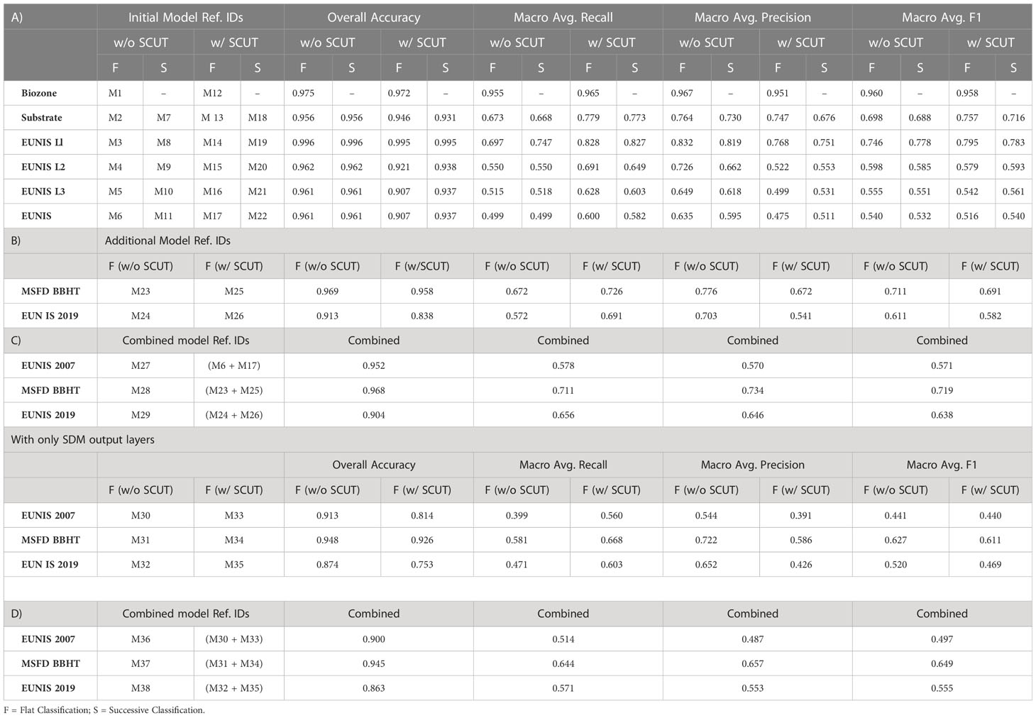
Table 1 With all available data.

3.1 Identification of optimal benthic habitat modelling strategy

Initially, to establish the optimal strategy for classifying benthic habitats with the available data, several modelling approaches were trialled. The EUNIS 2007 classification as provided by the EUSeaMap was used as an example target habitat classification system, and all of the data from the species distribution model inputs and outputs described previously in sections 2.2 and 2.3 were used as inputs to these models. RF classifiers were developed using both “flat” and “sequential” modelling approaches with the unaltered (unbalanced) training dataset as well as a balanced training dataset obtained using SCUT. Individual classifiers were developed for the highest level of EUNIS 2007 available in the EUSeaMap data, as well as the habitat descriptors of substrate and biozone and, where applicable, the lower “parent” levels of the EUNIS hierarchy derived as described previously. Based on model classification of the retained test dataset, all of these RF classifiers (M1-M22) were capable of classifying habitat descriptors and benthic habitats according to EUNIS 2007 across all levels of the classification system’s hierarchy with very high overall accuracy (mean 0.956 ± 0.027). When using the original unbalanced data for model training, both flat and successive modelling approaches had almost identical performances in terms of accurately predicting EUNIS 2007 habitats in the test dataset, however for models trained using the balanced datasets obtained with SCUT, the successive approach achieved slightly higher accuracy than the flat approach (0.937 vs 0.907 respectively). Compared to models trained on the unaltered (unbalanced) datasets, all models trained on the datasets obtained with SCUT exhibited higher R_MA values, but lower values of accuracy and P_MA. The model with the highest P_MA (0.635) was M6, which was a flat model trained on the original unaltered training dataset; this model had an R_MA of 0.499 and a F1_MA of 0.540. The model with the highest R_MA (0.600) was M17, which was a flat model trained on the SCUT balanced training dataset; this model had a P_MA of 0.475 and a F1_MA of 0.516. As as RF model is simply an ensemble of decision trees, it is possible to combine RF models to obtain a single large ensemble comprised of all the decision trees from all constituent RF models. Combining RF models M6 and M17, a large ensemble model (M27) was obtained which predicted EUNIS habitats in the EUSeaMap test data set with an accuracy of 0.952, a R_MA of 0.578, a P_MA of 0.570, and a F1_MA of 0.571; while these accuracy, R_MA, and P_MA metrics are between the ranges of values obtained for RF models M6 and M11, the F1_MA for M27 is higher than that of either constituent model, suggesting that this combined model achieves a more optimal balance between recall and precision than either M6 or M11.

As discussed previously, macro-averaged metrics assign equal importance to all classes, resulting in less prevalent classes having a disproportionately large impact on the metrics relative to their representation in the test dataset. This effect is illustrated in Figure 1, which shows step-wise evaluations of the macro-averaged precisions, recalls, and F1-scores for models M6, M11, and M27 (y-axis) against the sum of the prevalences of classes considered at each step (x-axis), i.e. $\frac{1}{n}{\sum }_{i=1}^n{m}_i$vs ${\sum }_{i=1}^n{p}_i$ with points plotted for each i of n total classes ordered by decreasing prevalence in the test dataset, where m_i is the by-class precision, recall, or F1-score of the i^th class, and p_i is the prevalence of the i^th class. As can be observed, 10 habitat classes comprise ~99% of the test dataset, and there is a substantial difference in macro-average metrics calculated on the basis of this 99% compared to macro-averaged metrics calculated using the entire test dataset; taking model M27 as an example, P_MA falls from 0.801 to 0.570, R_MA falls from 0.846 to 0.578, and the F1_MA falls from 0.821 to 0.571. This again highlights the complexity of evaluating model performances and demonstrates that no single metric considered in isolation can adequately evaluate model performance.

FIGURE 1

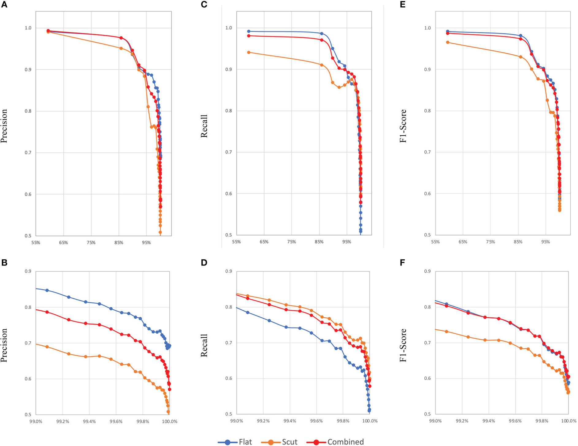
Figure 1 Comparison of changes in model evaluation metrics based on ordering habitats from highest to lowest prevalence and computing macro-averaged precision, recall and F1-scores sequentially for a combined model (M27) and its constituent models (M6 and M17) classifying benthic habitats according to the EUNIS 2007 habitat classification system. (A, C, E) show changes in precision, recall, and F1-score, respectively. For a closer look, (B, D, F) show zoomed-in views of these graphs, respectively, with the x-axes truncated at 99%.

3.2 Classification errors

As described previously, all off-diagonal elements of the confusion matrices used for model evaluation were considered classification errors. While this is the usual manner of determining misclassifications for the purposes of model evaluation, there are several confounding factors which might result in model performance being underestimated as a result of this. For example, because of its hierarchical structure, habitats can be labelled at different levels of the EUNIS classification, meaning there are multiple labels which could be correctly applied to any given habitat, however this is not considered by any of the metrics calculated to assess model performance. Taking as an example the confusion matrix for model M27 (Figure S3) which shows that ~68% of habitats classified as A5 in the EUSeaMap test dataset were identified as such by the model, with A5.15 accounting for ~15% of model predictions, A5.14 for ~4%, A5.27 for ~3%, and A5.34 and A5.611 for ~1% each. In effect, this means that 92.6% of habitats classified as A5 in the EUSeaMap test dataset were identified by the model as A5 or subsets thereof, however without better testing data (e.g. derived from ground truthing) it would be impossible to determine the true accuracy of these predictions. A similar case exemplifying this issue is that, while ~64% of the instances of A6.611 (Deep-sea Lophelia pertusa reefs) in the test dataset were correctly classified by model M27, ~27% were classified as A6 (Deep-sea bed); while this is not technically incorrect per se, it was considered a misclassification for the purposes of model evaluation. Confusion matrices for models M28, M29, M36, M37, and M38 are also provided in the supplementary material as Figures S4–S8, respectively.

For some habitat classes, the paucity of data available for model training and testing is also a significant limitation. For example, class A3.3, Atlantic and Mediterranean low energy infralittoral rock, was very sparsely represented in the training and test data with only 29 and 7 instances in the respective datasets. As the confusion matrix for model 27 (Figure S3) shows, no instances of A3.3 in the test set were correctly predicted; of the 7 instances of A3.3 in the test set, 4 (~43%) were predicted as A4.33, Faunal communities on deep low energy circalittoral rock, 1 (~14%) was predicted as A4.3, Atlantic and Mediterranean low energy circalittoral rock, 1 (~14%) was predicted as A5.43, Infralittoral mixed sediments, 1 (~14%) was predicted as A3.2 Atlantic and Mediterranean moderate energy infralittoral rock, and 1 (~14%) was predicted as A5.25 or A5.26, Circalittoral fine sand or Circalittoral muddy sand. Model 27 thus correctly predicted a rock seabed substrate in ~71% of cases, but confused the infralittoral and circalittoral zones. The infralittoral zone is defined as being the area of the photic zone which is permanently submerged, while the circalittoral extends from the bottom of the infralittoral to the wave-base (the maximum depth at which there is wave disturbance) (Coggan et al., 2011). In the EUSeaMap, the transition between the infralittoral and circalittoral zones is necessarily delineated by hard thresholds, however given the high spatiotemporal variability of both the photic zone (Lee et al., 2007; Saulquin et al., 2013) and the depth to the wave-base (Roland and Ardhuin, 2014; Henriques et al., 2015), this transition in reality occurs across a gradual environmental gradient, so any model confusion in differentiating between these zones given limited input data is perhaps unsurprising.

3.3 Models for other habitat classification systems

With an optimal modelling strategy identified, two further RF models were developed using the same methodology to classify habitats according to i) the MSFD BBHT classification and ii) the EUNIS 2019 classification. Combining RF models M23 and M25, a large ensemble model (M28) was obtained which predicted MSFD BBHTs in the EUSeaMap test data set with an accuracy of 0.968, a R_MA of 0.711, a P_MA of 0.734, and a F1_MA of 0.719; while these accuracy, R_MA, and P_MA metrics are between the ranges of values obtained for RF models M23 and M25, the F1_MA for M28 is higher than that of either constituent model, as was the case for the combined EUNIS 2007 model, suggesting that this combined model for MSFD BBHT also achieved a more optimal balance between recall and precision than either model M23 or M25 alone. Similarly, combining RF models M24 and M26, a large ensemble model (M29) was obtained which predicted benthic habitats in the EUSeaMap test data set according to the EUNIS 2019 classification system with an accuracy of 0.904, a R_MA of 0.654, a P_MA of 0.646, and a F1_MA of 0.638, and again, these accuracy, R_MA, and P_MA metrics were between the ranges of values obtained for RF models M24 and M26, with the F1_MA for M29 also being higher than that of either constituent model.

3.4 Models built solely with species distribution model outputs

RF models were also developed using only SDM outputs as proxies for habitats. Combining RF models M30 and M33, a large ensemble model, M36, was obtained, which predicted benthic habitats in the EUSeaMap test data set according to the EUNIS 2007 classification system with an accuracy of 0.900, a R_MA of 0.514, a P_MA of 0.487, and a F1_MA of 0.497. Similarly, combining RF models M31 and M34, a large ensemble model, M37, was obtained, which predicted MSFD BBHTs in the EUSeaMap test data set with an accuracy of 0.945, a R_MA of 0.644, a P_MA of 0.657, and a F1_MA of 0.649. And finally, combining RF models M32 and M35, a large ensemble model, M38, was obtained, which predicted benthic habitats in the EUSeaMap test data set according to the EUNIS 2019 classification system with an accuracy of 0.863, a R_MA of 0.571, a P_MA of 0.563, and a F1_MA of 0.611. As observed previously, in all cases the accuracy, R_MA, and P_MA values observed for the large ensemble models were between the ranges of values obtained for their constituent RF models, however the F1_MA scores were always higher than that of either constituent model. Given that RF models had significantly fewer features to use as predictors, some reduction in these metrics would be expected, and as can be seen in Figure 2, the accuracy and macro averaged metrics for models developed with only the SDM output data to classify habitats according to the EUNIS 2007 classification system were lower than those developed using both the SDM input and output data, but only slightly so; in absolute terms, when considering all habitat classes, the accuracy of M36 was reduced by just 0.052 compared to M27, with the R_MA, P_MA and F1_MA reduced by 0.064, 0.083, and 0.079 respectively.

FIGURE 2

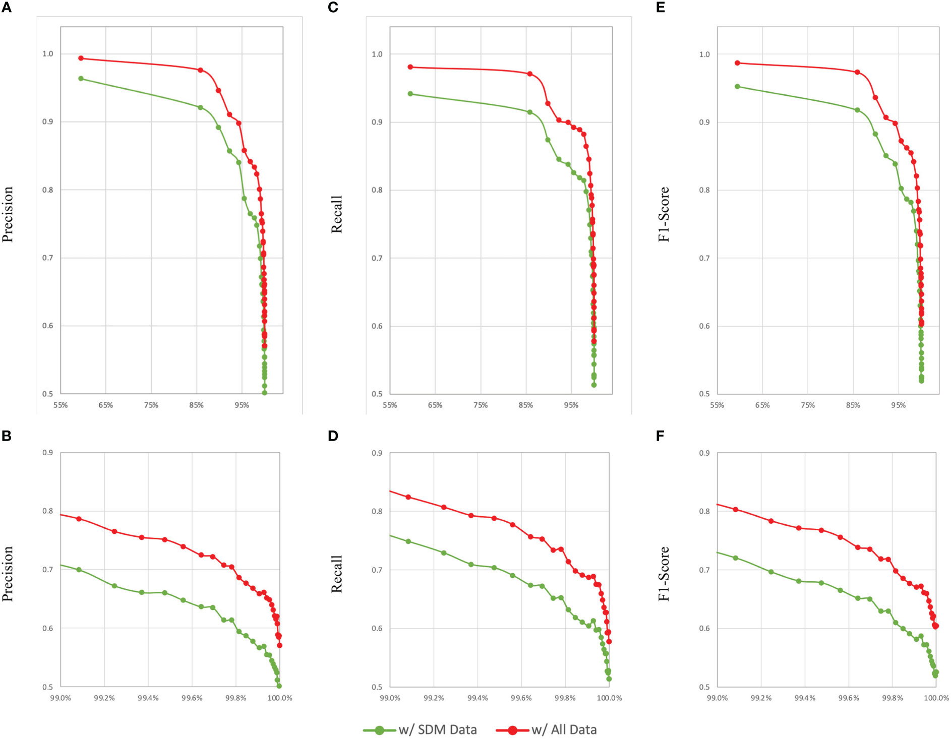
Figure 2 Comparison of changes in model evaluation metrics based on ordering habitats from highest to lowest prevalence and computing macro-averaged precision, recall and F1-scores sequentially for a model developed using all available data as RF inputs (M27) and a model developed using only SDM outputs as RF inputs (M36) to classify benthic habitats according to the EUNIS 2007 habitat classification system. (A, C, E) show changes in precision, recall, and F1-score, respectively. For a closer look, (B, D, F) show zoomed-in views of these graphs, respectively, with the x-axes truncated at 99%.

3.5 Extending habitat classification systems across ocean basins

As a demonstration of the methodology’s utility, the habitat classification systems used by the EUSeaMap were subsequently extended to the entire North Atlantic Basin using the best performing models for each classification system. Figure 3 shows the EUNIS 2007 habitat classification of the North Atlantic Basin using model M27, while Supplementary Figures S1, S2 show the MSFD BBHT and EUNIS 2019 habitat classifications of the North Atlantic Basin using models M28 and M29, respectively. Due to the scale of the maps and the large number of habitats presented, these maps are intended only to indicate the extents of the areas classified with the legends intended only to indicate the number and variety of habitat classes.

FIGURE 3

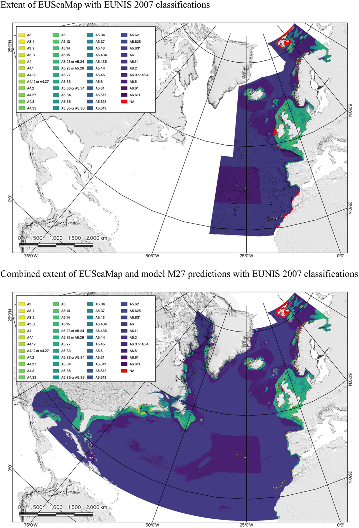
Figure 3 Maps comparing the EUSeaMap classified according to the EUNIS 2007 habitat classification (top) with the output of RF model M27, which extends this classification across the North Atlantic Basin (bottom).

While the models were shown to have excellent predictive power on the test dataset, it is very important to note the caveat that the North Atlantic Basin comprises many distinct biogeographic regions (Schumacher et al., 2022), and, as the habitat classifications represented in the EUSeaMap were developed for benthic habitats in the North East Atlantic, they may not be applicable outside European waters (Galparsoro et al., 2012), especially if the input data used to train the RF models are not representative of the full range of biogeographic conditions found throughout the basin. To address this issue, it might be necessary to develop separate models for different parts of the North Atlantic Basin and possibly to expand the habitat classification systems used, however, despite these limitations, marine habitats in different biogeographical regions can be highly similar in many ways, and thus can react similarly when subjected to pressures concomitant with human activities. For example, despite their very distinct biogeographies, shallow tropical coral reefs and their deep-sea cold-water counterparts share many similarities in terms of ecosystem function and habitat sensitivity to anthropogenic impacts; both habitats provide important habitat for a diverse array of marine species, and both are sensitive to anthropogenic impacts, such as physical disturbance, pollution, and climate change.

Notwithstanding the caveats above, this study demonstrates that the species composition in a given area (or rather a subset thereof) can serve as a useful indicator of habitat, and this is not solely predicated on the presence or absence of given species in that area, but rather the unique “fingerprint” of modelled relative probabilities of species occurrences therein. Thus, the relative probability of species occurrence whether low or high, provides useful information for the purposes of habitat classification.

4 Conclusions

Knowledge of seabed habitat distribution provides an essential foundation for the conservation and sustainable utilisation of marine resources as well as the effective management of maritime activities. Maps of the areal extents and distributions of benthic habitats allow for informed decision making regarding the management of living and non-living resources present on the seafloor, enabling relevant authorities to 1) optimally manage spatial and temporal overlaps between multiple human activities and habitats/species particularly sensitive to the anthropogenic impacts associated therewith (Andersen et al., 2018; Baker and Harris, 2020), 2) design Marine Protected Areas which are, as recommended by the Convention on Biological Diversity, “ecologically representative and well-connected” (CBD, 2021), and 3) use environmental accounting approaches to integrate the ecological and socio-economic value of natural capital into Marine Spatial Planning processes (Picone et al., 2017; Bouwma et al., 2018). The use of species distribution modelling to develop full-coverage maps of species habitat suitability over wide areas has become ubiquitous, however there is still the need for marine habitats to be classified according to widely used, univocal habitat classification systems. This study presents a globally applicable, easily reproducible supervised machine learning approach by which to use the outputs of species distribution models to extend existing habitat classification systems over larger areas, thus maximizing the potential use of current evidence-based management decision tools.

Data availability statement

The raw data supporting the conclusions of this article will be made available by the authors, without undue reservation.

Author contributions

AG and OC conceived the study. OC undertook the modelling and wrote the first draft of manuscript. Both authors contributed to the article and approved the submitted version.

Funding

This project has received funding from the European Union’s Horizon 2020 research and innovation programme under grant agreement No. 678760 (ATLAS) and Science Foundation Ireland grant SFI/12/RC/2302 to MaREI - the Science Foundation Ireland Research Centre for Energy, Climate and Marine (www.marei.ie). The output reflects only the authors' views, and the European Union, Science Foundation Ireland, or Marine Institute cannot be held responsible for any use that may be made of the information contained therein. OC is supported by the ‘CÓIR – ‘Changing Ocean IReland: Forecasting Biodiversity and Ecosystem Response’ Marine Institute Fellowship (Grant-Aid Agreement No. SPDOC/CC/20/001) funded under the Marine Research Programme Ocean Ecosystems and Climate Call by the Irish Government.

Conflict of interest

The authors declare that the research was conducted in the absence of any commercial or financial relationships that could be construed as a potential conflict of interest.

Publisher’s note

All claims expressed in this article are solely those of the authors and do not necessarily represent those of their affiliated organizations, or those of the publisher, the editors and the reviewers. Any product that may be evaluated in this article, or claim that may be made by its manufacturer, is not guaranteed or endorsed by the publisher.

Author disclaimer

The output reflects only the authors' views, and the European Union, Science Foundation Ireland, or Marine Institute cannot be held responsible for any use that may be made of the information contained therein.

Supplementary material

The Supplementary Material for this article can be found online at: https://www.frontiersin.org/articles/10.3389/fmars.2023.1139425/full#supplementary-material

References

Agrawal A., Viktor H. L., Paquet E. (2015). SCUT: Multi-class imbalanced data classification using SMOTE and cluster-based undersampling, in: 2015 7th international joint conference on knowledge discovery, knowledge engineering and knowledge management (IC3K). 2015 7th Int. Joint Conf. Knowledge Discovery Knowledge Eng. Knowledge Manage. (IC3K), 226–234.

Google Scholar

Alvarez S. A. (2002). An exact analytical relation among recall, precision, and classification accuracy in information retrieval (Boston College, Boston) Technical Report BCCS-02-01, pp.1–22. Available at: http://www.cs.bc.edu/~alvarez/APR/aprformula.pdf

Google Scholar

Andersen J. H., Manca E., Agnesi S., Al-Hamdani Z., Lillis H., Mo G., et al. (2018). European Broad-scale seabed habitat maps support implementation of ecosystem-based management. Open J. Ecol. 08, 86–103. doi: 10.4236/oje.2018.82007

CrossRef Full Text | Google Scholar

Anderson J. T., Holliday V., Kloser R., Reid D., Simard Y., Brown C. J., et al. (2007). Acoustic seabed classification of marine physical and biological landscapes (International Council for the Exploration of the Sea Copenhagen). doi: 10.17895/ices.pub.5453

CrossRef Full Text | Google Scholar

Auster P. J., Joy K., Valentine P. C. (2001). Fish species and community distributions as proxies for seafloor habitat distributions: The stellwagen bank national marine sanctuary example (Northwest Atlantic, gulf of Maine). Environ. Biol. Fishes 60, 331–346. doi: 10.1023/A:1011022320818

CrossRef Full Text | Google Scholar

Baker E. K., Harris P. T. (2020). “Chapter 2 - habitat mapping and marine management,” in Seafloor geomorphology as benthic habitat, 2nd ed. Eds. Harris P. T., Baker E. (Elsevier), 17–33. doi: 10.1016/B978-0-12-814960-7.00002-6

CrossRef Full Text | Google Scholar

Begon M., Townsend C. R. (2020). Ecology: From individuals to ecosystems (John Wiley & Sons). Available at: https://www.wiley.com/en-us/Ecology%3A+From+Individuals+to+Ecosystems%2C+5th+Edition-p-9781119279358

Google Scholar

Borland H. P., Gilby B. L., Henderson C. J., Leon J. X., Schlacher T. A., Connolly R. M., et al. (2021). The influence of seafloor terrain on fish and fisheries: A global synthesis. Fish Fish. 22, 707–734. doi: 10.1111/faf.12546

CrossRef Full Text | Google Scholar

Bouwma I., Schleyer C., Primmer E., Winkler K. J., Berry P., Young J., et al. (2018). Adoption of the ecosystem services concept in EU policies. Ecosyst. Serv. 29, 213–222. doi: 10.1016/j.ecoser.2017.02.014

CrossRef Full Text | Google Scholar

Breiman L. (2001). Random forests. Mach. Learn. 45, 5–32. doi: 10.1023/A:1010933404324

CrossRef Full Text | Google Scholar

Brown C. J., Blondel P. (2009). Developments in the application of multibeam sonar backscatter for seafloor habitat mapping. Appl. Acoust. 70, 1242–1247. doi: 10.1016/j.apacoust.2008.08.004

CrossRef Full Text | Google Scholar

Brown C. J., Smith S. J., Lawton P., Anderson J. T. (2011). Benthic habitat mapping: A review of progress towards improved understanding of the spatial ecology of the seafloor using acoustic techniques. Estuar. Coast. Shelf Sci. 92, 502–520. doi: 10.1016/j.ecss.2011.02.007

CrossRef Full Text | Google Scholar

CBD (2021). First draft of the post-2020 global biodiversity framework (UNEP). Available at: https://www.cbd.int/doc/c/914a/eca3/24ad42235033f031badf61b1/wg2020-03-03-en.pdf.

Google Scholar

Chawla N. V., Bowyer K. W., Hall L. O., Kegelmeyer W. P. (2002). SMOTE: Synthetic minority over-sampling technique. J. Artif. Intell. Res. 16, 321–357. doi: 10.1613/jair.953

CrossRef Full Text | Google Scholar

Coggan R., James C., Pearce B., Plim J. (2011). “Using the EUNIS habitat classification system in broadscale regional mapping: some problems and potential solutions from case studies in the English channel,” in ICES Annual Science Conference. Available at: http://ices.dk/sites/pub/CM%20Doccuments/CM-2011/G/G0311.pdf

Google Scholar

Cooper A. J., Spearman J. (2017). “Validation of a TELEMAC-3D model of a seamount,” in Proc. XXIVth TELEMAC-MASCARET User Conf, Graz Univ. Technol. Austria, 17 20 Oct. 2017. 17–22. Available at: https://hdl.handle.net/20.500.11970/104505

Google Scholar

Cormier R., Kelble C. R., Anderson M. R., Allen J. I., Grehan A., Gregersen Ó. (2017). Moving from ecosystem-based policy objectives to operational implementation of ecosystem-based management measures. ICES J. Mar. Sci. 74, 406–413. doi: 10.1093/icesjms/fsw181

CrossRef Full Text | Google Scholar

Costello M. J., Coll M., Danovaro R., Halpin P., Ojaveer H., Miloslavich P. (2010). A census of marine biodiversity knowledge, resources, and future challenges. PloS One 5, e12110. doi: 10.1371/journal.pone.0012110

PubMed Abstract | CrossRef Full Text | Google Scholar

Cutler F., Wiener R. (2022). randomForest: Breiman and cutler’s random forests for classification and regression. R package version 4.7-1.

Google Scholar

Davies C. E., Moss D., Hill M. O. (2004). EUNIS habitat classification revised 2004. Rep. Eur. Environ. Agency-Eur. Top. Cent. Nat. Prot. Biodivers, 127–143.

Google Scholar

Diaz R. J., Solan M., Valente R. M. (2004). A review of approaches for classifying benthic habitats and evaluating habitat quality. J. Environ. Manage. 73, 165–181. doi: 10.1016/j.jenvman.2004.06.004

PubMed Abstract | CrossRef Full Text | Google Scholar

Dolan M. F. J., Van Lancker V., Guinan J., Al-Hamdani Z., Leth J., Thorsnes T. (2012). Terrain characterization from bathymetry data at various resolutions in European waters - experiences and recommendations. NGU report, vol. 2012045, NGU.

Google Scholar

EUNIS marine habitat classification 2019 including crosswalks — European Environment Agency. Available at: https://www.eea.europa.eu/data-and-maps/data/eunis-habitat-classification-1/eunis-marine-habitat-classification-review-2019/eunis-marine-habitat-classification-2019 (Accessed 10.19.22).

Google Scholar

Evans D., Aish A., Boon A., Condé S., Connor D., Gelabert E. M. N., et al. (2016). Revising the marine section of the EUNIS habitat classification-report of a workshop held at the European topic centre on biological diversity, 12 & 13 may 2016 (ETCBD Rep) EEA. Available at: https://www.eea.europa.eu/data-and-maps/data/eunis-habitat-classification/documentation/revising-the-marine-section-of/download

Google Scholar

Fennel K., Mattern J. P., Doney S. C., Bopp L., Moore A. M., Wang B., et al. (2022). Ocean biogeochemical modelling. Nat. Rev. Methods Primer 2, 1–21. doi: 10.1038/s43586-022-00154-2

CrossRef Full Text | Google Scholar

Foley M. M., Halpern B. S., Micheli F., Armsby M. H., Caldwell M. R., Crain C. M., et al. (2010). Guiding ecological principles for marine spatial planning. Mar. Policy 34, 955–966. doi: 10.1016/j.marpol.2010.02.001

CrossRef Full Text | Google Scholar

Franklin J. (2013). Species distribution models in conservation biogeography: developments and challenges. Divers. Distrib. 19, 1217–1223. doi: 10.1111/ddi.12125

CrossRef Full Text | Google Scholar

Galparsoro I., Borja A., Uyarra M. C. (2014). Mapping ecosystem services provided by benthic habitats in the European north Atlantic ocean. Front. Mar. Sci. 1. doi: 10.3389/fmars.2014.00023

PubMed Abstract | CrossRef Full Text | Google Scholar

Ganz K. (2021). Scutr: Balancing multiclass datasets for classification tasks. R Package version 0.1.2.. Available at: https://CRAN.R-project.org/package=scutr.

Google Scholar

Galparsoro I., Connor D. W., Borja Á., Aish A., Amorim P., Bajjouk T., et al. (2012). Using EUNIS habitat classification for benthic mapping in European seas: Present concerns and future needs. Mar. pollut. Bull. 64, 2630–2638. doi: 10.1016/j.marpolbul.2012.10.010

PubMed Abstract | CrossRef Full Text | Google Scholar

GEBCO (General Bathymetric Chart of the Oceans) (2022) Release of the GEBCO_2022 grid. Available at: https://www.gebco.net/news_and_media/gebco_2022_grid_release.html (Accessed 01.10.22).

Google Scholar

Gholamy A., Kreinovich V., Kosheleva O. (2018). Why 70/30 or 80/20 relation between training and testing sets: A pedagogical explanation. Dep. Tech. Rep. CS. 1209. Available at: https://scholarworks.utep.edu/cs_techrep/1209

Google Scholar

Goes E. R., Brown C. J., Araújo T. C. (2019). Geomorphological classification of the benthic structures on a tropical continental shelf. Front. Mar. Sci. 6. doi: 10.3389/fmars.2019.00047

CrossRef Full Text | Google Scholar

Grandini M., Bagli E., Visani G. (2020). Metrics for multi-class classification: an overview. arXiv preprint. arXiv:2008.05756. doi: 10.48550/arXiv.2008.05756

PubMed Abstract | CrossRef Full Text | Google Scholar

Grehan A. J., Arnaud-Haond S., D`Onghia G., Savini A., Yesson C. (2017). Towards ecosystem based management and monitoring of the deep Mediterranean, north-East Atlantic and beyond. Deep-Sea Res. Part II Top. Stud. Oceanogr. 145, 1–7. doi: 10.1016/j.dsr2.2017.09.014

CrossRef Full Text | Google Scholar

Hasan R. C., Ierodiaconou D., Laurenson L., Schimel A. (2014). Integrating multibeam backscatter angular response, mosaic and bathymetry data for benthic habitat mapping. PloS One 9, e97339. doi: 10.1371/journal.pone.0097339

PubMed Abstract | CrossRef Full Text | Google Scholar

Hastie T., Tibshirani R. (1987). Generalized additive models: Some applications. J. Am. Stat. Assoc. 82, 371–386. doi: 10.1080/01621459.1987.10478440

CrossRef Full Text | Google Scholar

Henriques V., Guerra M. T., Mendes B., Gaudêncio M. J., Fonseca P. (2015). Benthic habitat mapping in a Portuguese marine protected area using EUNIS: An integrated approach. J. Sea Res. MeshAtlantic: Mapp. Atlantic Area Seabed Habitats Better Mar. Manage. 100, 77–90. doi: 10.1016/j.seares.2014.10.007

CrossRef Full Text | Google Scholar

Hijmans R. J., van Etten J. (2016). Raster: Geographic data analysis and modeling. R Package version 3.6-3.

Google Scholar

Hiscock K. (2020). “Chapter 26 - using science effectively: Selection, design and management of marine protected areas,” in Marine protected areas. Eds. Humphreys J., Clark R. W. E. (Elsevier), 507–523. doi: 10.1016/B978-0-08-102698-4.00026-5

CrossRef Full Text | Google Scholar

Hutchinson G. E. (1944). Limnological studies in connecticut. VII. a critical examination of the supposed relationship between phytoplakton periodicity and chemical changes in lake waters. Ecology 25, 3–26. doi: 10.2307/1930759

CrossRef Full Text | Google Scholar

Hutchinson G. E. (1957). Concluding remarks. Cold Spring Harb. Symp. Quant. Biol. 22, 415–427. doi: 10.1101/SQB.1957.022.01.039

CrossRef Full Text | Google Scholar

James G., Witten D., Hastie T., Tibshirani R. (2013). An introduction to statistical learning (Springer). doi: 10.1007/978-1-0716-1418-1

CrossRef Full Text | Google Scholar

Kenny A. J., Cato I., Desprez M., Fader G., Schüttenhelm R. T. E., Side J. (2003). An overview of seabed-mapping technologies in the context of marine habitat classification☆. ICES J. Mar. Sci. 60, 411–418. doi: 10.1016/S1054-3139(03)00006-7

CrossRef Full Text | Google Scholar

Kuhn M., Wing J., Weston S., Williams A., Keefer C., Engelhardt A., et al. (2022). Caret: Classification and regression training. R package version 6.0-91.

Google Scholar

Lamarche G., Orpin A. R., Mitchell J. S., Pallentin A. (2016). Benthic habitat mapping, in: Biological sampling in the deep Sea (John Wiley & Sons, Ltd), 80–102. doi: 10.1002/9781118332535.ch5

CrossRef Full Text | Google Scholar

Lambeck R. J. (1997). Focal species: A multi-species umbrella for nature conservation. Conserv. Biol. 11, 849–856. doi: 10.1046/j.1523-1739.1997.96319.x

CrossRef Full Text | Google Scholar

Lee Z., Weidemann A., Kindle J., Arnone R., Carder K. L., Davis C. (2007). Euphotic zone depth: Its derivation and implication to ocean-color remote sensing. J. Geophys. Res. Oceans 112. doi: 10.1029/2006JC003802

CrossRef Full Text | Google Scholar

Lucieer V., Huang Z., Siwabessy J. (2016). Analyzing uncertainty in multibeam bathymetric data and the impact on derived seafloor attributes. Mar. Geod. 39, 32–52. doi: 10.1080/01490419.2015.1121173

CrossRef Full Text | Google Scholar

Manning C., Schutze H. (1999). Foundations of statistical natural language processing (MIT Press). Available at: https://mitpress.mit.edu/9780262133609/

Google Scholar

McLeod K. L., Lubchenco J., Palumbi S. R., Rosenberg A. A. (2005). Scientific consensus statement on marine ecosystem-based management. Signed By 221, 21.

Google Scholar

Melo-Merino S. M., Reyes-Bonilla H., Lira-Noriega A. (2020). Ecological niche models and species distribution models in marine environments: A literature review and spatial analysis of evidence. Ecol. Model. 415, 108837. doi: 10.1016/j.ecolmodel.2019.108837

CrossRef Full Text | Google Scholar

Morato T., González-Irusta J. M., Domínguez-Carrió C., Wei C., Davies A., Sweetman A. K., et al. (2019). Climate-induced changes in the suitable habitat of cold-water corals and commercially important deep-sea fishes in the north Atlantic. doi: 10.1594/PANGAEA.910319

CrossRef Full Text | Google Scholar

Morato T., González-Irusta J.-M., Dominguez-Carrió C., Wei C.-L., Davies A., Sweetman A. K., et al. (2020). Climate-induced changes in the suitable habitat of cold-water corals and commercially important deep-sea fishes in the north Atlantic. Glob. Change Biol. 26, 2181–2202. doi: 10.1111/gcb.14996

CrossRef Full Text | Google Scholar

Narayanaswamy B. E., Bett B. J., Lamont P. A., Rowden A. A., Bell E. M., Menot L. (2016). Corers and grabs, in: Biological sampling in the deep Sea (John Wiley & Sons, Ltd), 207–227. doi: 10.1002/9781118332535.ch10

CrossRef Full Text | Google Scholar

Opitz J., Burst S. (2019). Macro f1 and macro f1. arXiv preprint. arXiv:1911.03347.

Google Scholar

Pebesma E., Bivand R., Rowlingson B., Gomez-Rubio V., Hijmans R., Sumner M., et al. (2022). Sp: Classes and methods for spatial data. R package version 1.4-6

PubMed Abstract | Google Scholar

Phillips S. J., Anderson R. P., Dudík M., Schapire R. E., Blair M. E. (2017). Opening the black box: an open-source release of maxent. Ecography 40, 887–893. doi: 10.1111/ecog.03049

CrossRef Full Text | Google Scholar

Phillips S. J., Anderson R. P., Schapire R. E. (2006). Maximum entropy modeling of species geographic distributions. Ecol. Model. 190, 231–259. doi: 10.1016/j.ecolmodel.2005.03.026

CrossRef Full Text | Google Scholar

Picone F., Buonocore E., D’Agostaro R., Donati S., Chemello R., Franzese P. P. (2017). Integrating natural capital assessment and marine spatial planning: A case study in the Mediterranean sea. Ecol. Model. 361, 1–13. doi: 10.1016/j.ecolmodel.2017.07.029

CrossRef Full Text | Google Scholar

Populus J., Vasquez M., Albrecht J., Manca E., Agnesi S., Al Hamdani Z., et al. (2017). EUSeaMap. a European broad-scale seabed habitat map. (Brest: Ifremer). doi: 10.13155/49975

CrossRef Full Text | Google Scholar

Probst P., Boulesteix A.-L., Bischl B. (2019a). Tunability: Importance of hyperparameters of machine learning algorithms. J. Mach. Learn. Res. 20, 1934–1965.

Google Scholar

Probst P., Wright M. N., Boulesteix A.-L. (2019b). Hyperparameters and tuning strategies for random forest. WIREs Data Min. Knowl. Discovery 9, e1301. doi: 10.1002/widm.1301

CrossRef Full Text | Google Scholar

Ramiro-Sánchez B., González-Irusta J. M., Henry L.-A., Cleland J., Yeo I., Xavier J. R., et al. (2019). Characterization and mapping of a deep-Sea sponge ground on the tropic seamount (Northeast tropical atlantic): Implications for spatial management in the high seas. Front. Mar. Sci. 6. doi: 10.3389/fmars.2019.00278

CrossRef Full Text | Google Scholar

Roland A., Ardhuin F. (2014). On the developments of spectral wave models: numerics and parameterizations for the coastal ocean. Ocean Dyn. 64, 833–846. doi: 10.1007/s10236-014-0711-z

CrossRef Full Text | Google Scholar

Rondinini C. (2011). Meeting the MPA network design principles of representativity and adequacy: Developing species-area curves for habitats (UK: Joint Nature Conservation Committee Peterborough).

Google Scholar

Saulquin B., Hamdi A., Gohin F., Populus J., Mangin A., d’Andon O. F. (2013). Estimation of the diffuse attenuation coefficient KdPAR using MERIS and application to seabed habitat mapping. Remote Sens. Environ. 128, 224–233. doi: 10.1016/j.rse.2012.10.002

CrossRef Full Text | Google Scholar

Scarponi P., Coro G., Pagano P. (2018). A collection of aquamaps native layers in NetCDF format. Data Brief 17, 292–296. doi: 10.1016/j.dib.2018.01.026

PubMed Abstract | CrossRef Full Text | Google Scholar

Schiele K. S., Darr A., Zettler M. L. (2014). Verifying a biotope classification using benthic communities – an analysis towards the implementation of the European marine strategy framework directive. Mar. pollut. Bull. 78, 181–189. doi: 10.1016/j.marpolbul.2013.10.045

PubMed Abstract | CrossRef Full Text | Google Scholar

Schumacher M., Huvenne V. A. I., Devey C. W., Arbizu P. M., Biastoch A., Meinecke S. (2022). The Atlantic ocean landscape: A basin-wide cluster analysis of the Atlantic near seafloor environment. Front. Mar. Sci. 9. doi: 10.3389/fmars.2022.936095

PubMed Abstract | CrossRef Full Text | Google Scholar

Shumchenia E. J., King J. W. (2010). Comparison of methods for integrating biological and physical data for marine habitat mapping and classification. Cont. Shelf Res. 30, 1717–1729. doi: 10.1016/j.csr.2010.07.007

CrossRef Full Text | Google Scholar

Sokolova M., Lapalme G. (2009). A systematic analysis of performance measures for classification tasks. Inf. Process. Manage. 45, 427–437. doi: 10.1016/j.ipm.2009.03.002

CrossRef Full Text | Google Scholar

Sunagawa S., Acinas S. G., Bork P., Bowler C., Eveillard D., Gorsky G., et al. (2020). Tara Oceans: towards global ocean ecosystems biology. Nat. Rev. Microbiol. 18, 428–445. doi: 10.1038/s41579-020-0364-5

PubMed Abstract | CrossRef Full Text | Google Scholar

Tillin H. M., Hull S. C., Tyler-Walters H. (2010). Development of a sensitivity matrix (pressures-MCZ/MPA features). Report to the Department of Environment, Food and Rural Affairs from ABPMer, Southampton and the Marine Life Information Network (MarLIN) Plymouth: Marine Biological Association of the UK. Defra Contract No. MB0102 Task 3A, Report No. 22

Google Scholar

Tyler-Walters H., Tillin H. M., Perry F., Stamp T., d’Avack E. A. S. (2018). Marine evidence-based sensitivity assessment (MarESA)–a guide. Plymouth: Marine Biological Association of the UK.

Google Scholar

Vasquez M., Allen H., Manca E., Castle L., Lillis H., Agnesi S., et al. (2021). EUSeaMap 2021. a European broad-scale seabed habitat map. Technical Report. doi: 10.13155/83528

CrossRef Full Text | Google Scholar

Wei C.-L., González-Irusta J. M., Domínguez-Carrió C., Morato T. (2020). Set of terrain (static in time) and environmental (dynamic in time) variables used as candidate predictors of present-day, (1951-2000) and future, (2081-2100) suitable habitat of cold-water corals and deep-sea fishes in the north Atlantic. doi: 10.1594/PANGAEA.911117

CrossRef Full Text | Google Scholar

Wilson M. F. J., O’Connell B., Brown C., Guinan J. C., Grehan A. J. (2007). Multiscale terrain analysis of multibeam bathymetry data for habitat mapping on the continental slope. Mar. Geod. 30, 3–35. doi: 10.1080/01490410701295962

CrossRef Full Text | Google Scholar