Simulations of ocean deoxygenation in the historical era: insights from forced and coupled models

1 Introduction

Dissolved oxygen (O₂) sustains aerobic life in the ocean’s interior and plays a critical role in the ocean carbon and nitrogen cycles (e.g. Codispoti, 1995). Changes in O₂ levels have a major influence on ecosystem habitats and biogeochemistry throughout the water column (Morel and Price, 2003; Vaquer-Sunyer and Duarte, 2008; Keeling et al., 2010; Deutsch et al., 2015; Deutsch et al., 2022; Morée et al., 2023). One such change of particular concern is ocean “deoxygenation”, the long-term decline of O₂ content due to anthropogenic climate change, which, along with ocean warming and acidification, represents a major threat to marine biodiversity and fisheries in the 21^st Century (Gruber, 2011; Mora et al., 2013). Analysis from the 6^th Coupled Model Intercomparison Project (CMIP6) (Eyring et al., 2016) suggests that global warming will lead to about 3−4% decline in the global oceanic O₂ content by the end of the 21^st century (Kwiatkowski et al., 2020), and synthesis of observations indicate that about 1−2% of the global O₂ inventory has already been lost since the mid 20^th century (Ito et al., 2017; Schmidtko et al., 2017; Ito, 2022). While global open-ocean deoxygenation is largely driven by global warming, coastal oceans also experience deoxygenation caused by increased loading of nutrients (Breitburg et al., 2018) and the expansion of oxygen minimum zones (OMZs) (Breitburg et al., 2018; Levin, 2018).

The decrease in the oceanic O₂ content is driven by two key processes. First, ocean warming leads to a decrease in gas solubility, reducing the ability of surface waters to absorb O₂ (Keeling and Garcia, 2002). Second, warming further stratifies the upper ocean, reducing ventilation rates and weakening the supply of O₂ from the surface into the interior ocean (Bopp et al., 2002; Rhein et al., 2017; Tjiputra et al., 2018). Changes in ocean productivity and remineralization may also contribute to or compensate for these O₂ changes, but their overall effects in current models are relatively small compared to the physical drivers (Bopp et al., 2017). While Earth System Models (ESMs) largely project a reduction in the global oceanic O₂ content in response to warming, major challenges and discrepancies remain. The mechanisms and individual contribution of processes regulating these O₂ changes, for instance, differ across regions and models, leading to major uncertainties in the attribution and detection of observed O₂ trends and future projections (Bopp et al., 2013; Oschlies et al., 2018; Takano et al., 2018; Kwiatkowski et al., 2020; Buchanan and Tagliabue, 2021; Busecke et al., 2022; Tjiputra et al., 2023).

Recent studies suggest that ESMs may underestimate the observed interannual to decadal variability and long-term changes in the O₂ content and air-sea O₂ fluxes (Long et al., 2016; Eddebbar et al., 2017; Schmidtko et al., 2017; Oschlies et al., 2018). Models also struggle to reproduce the observed O₂ loss in the tropical basins (Stramma et al., 2012; Oschlies et al., 2017), likely due to pronounced biases in this region arising from poorly simulated or unresolved ocean processes (e.g. eddies and zonal equatorial jets) partly because of limitation in model resolutions (e.g. Figure 16 in Berthet et al., 2019), and a poorly constrained role for internal climate variability (Cabré et al., 2015; Berthet et al., 2019; Busecke et al., 2019; Ito et al., 2019; Laffoley and Baxter, 2019; Eddebbar et al., 2021). The observational estimates of ocean deoxygenation are also highly uncertain (Ito et al., 2017; Schmidtko et al., 2017; Ito, 2022), particularly in the tropical Oxygen Minimum Zones (OMZs) and the Southern Ocean where major spatial and temporal gaps exist. CMIP6 models showcase a more realistic ocean biogeochemistry than previous model generations due to improved representation of ocean physical and biogeochemical processes (Séférian et al., 2020; Canadell et al., 2021), but various challenges continue to hinder our assessment and understanding of ocean deoxygenation in both models and observations. The recent IPCC Sixth Assessment Report concluded with medium confidence that the subsurface O₂ content is projected to decrease in the next century (IPCC, 2019; Canadell et al., 2021; Cooley et al., 2022). The key question in the present study is whether ESMs simulate the observed ocean deoxygenation and O₂ variability during the historical era (defined here as changes in O₂ concentration or inventory in the past 5 decades) (Ito et al., 2017; Schmidtko et al., 2017; Ito, 2022).

In this study, we conduct a comprehensive assessment of simulations from CMIP6 models (Eyring et al., 2016) focusing on the global upper ocean (0-700m) deoxygenation in the past 5 decades (1960s-2010s) and how they compare to a recent observational dataset (Ito, 2022). Using model outputs from the Ocean Model Intercomparison Project 1 and 2 (OMIP1 and OMIP2) (Griffies et al., 2016; Orr et al., 2017) and CMIP6 Historical simulations, we examine how differences in model structure and atmospheric forcing (i.e. forced ocean-only vs coupled configurations) lead to differences in the simulated oceanic O₂ content response to the recent warming and compare these simulated trends to the most recently available gridded observational dataset (Ito, 2022). Various estimates of changes in ocean O₂ levels exist, varying mainly in their observational dataset construction methods (such as interpolation and gap filling procedures) (Helm et al., 2011; Ito et al., 2017; Schmidtko et al., 2017; Ito, 2022; Ito et al., 2023), though the availability of these products to the public via a community O₂ data platform and their comparison is still underway (e.g. Grégoire et al., 2021). We thus focus on the publicly available dataset from Ito, 2022 (and some complementary analysis based on the previous gridded O₂ dataset from 2017; Ito et al., 2017) and include a discussion on observational uncertainty in our comparison with the simulations. Our overall aim is to provide a comprehensive overview of model simulations of historical upper ocean deoxygenation and identify remaining challenges for the state-of-the-art models as guidelines for future coordinated efforts for ocean biogeochemistry simulations.

The structure of the paper is as follows. We first describe the CMIP6 models, configurations, observational dataset and data analysis methods used herein (Section 2). Section 3 outlines the OMIP simulations’ equilibrium states of sea water temperature and upper ocean O₂ along with key differences in climatological mean states of upper ocean O₂ between OMIP, CMIP6 Historical simulations and observations. In Section 4, we compare the observed and simulated changes in upper ocean O₂ over the past 5 decades, focusing on the upper 700m, where most of the O₂ changes and warming are expected in recent decades. We further evaluate the spatial characteristics of this O₂ change across the models and configurations and explore the drivers of the global O₂ loss. Finally, we conclude with a discussion on the future road map for coordinated modeling efforts to simulate the ocean O₂ cycle and outstanding uncertainties and discrepancies between models and observations.

2 Materials and methods

2.1 Ocean biogeochemistry simulations

We use model outputs from two sets of simulations from the forced ocean-only model simulations and a set of fully coupled Earth System Model (ESM) simulations from the CMIP6 Historical configuration (Séférian et al., 2020). More specifically, the forced ocean-only model simulations are based on the Ocean Model Intercomparison Project 1 (OMIP1) and Project 2 (OMIP2) protocols (Griffies et al., 2016; Orr et al., 2017; Tsujino et al., 2020) with two additional simulations based on the ECMWF ERA-20C and the NCEP-NCAR Reanalysis 1 atmospheric dataset (Kalnay et al., 1996; Poli et al., 2016). Forced oceanonly model simulations include ocean physics and biogeochemistry, with the atmosphere represented by non-interactive (and observation-derived) reanalysis fields of properties with bulk formulae to calculate ocean heat, moisture, and air-sea gas exchange fluxes, and momentum transfer. In contrast, fully coupled ESM simulations include the same representation of the ocean, but the atmosphere is a dynamical model that responds interactively to the ocean state driving it. In total, we analyze 17 models based on different configurations. We selected models that include an ocean biogeochemistry component and provide O₂ as model output. We use model outputs of sea water temperature (thetao) and salinity (so) (the names inside parentheses are the CMIP6 variable names) for calculating solubility driven changes in O₂ vs circulation and biology induced changes in O₂ (see section 2.3 for details).

A summary of the model and simulation information are shown in Table 1. The OMIP1 and OMIP2 simulations are based on the CORE-II protocol (Griffies et al., 2016; Tsujino et al., 2020), and use the CORE-II atmospheric forcing from 1948-2009 (Large and Yeager, 2009) and the JRA55-do atmospheric forcing from 1958-2018 (Tsujino et al., 2018), respectively. The JRA55-do atmospheric forcing covers a more recent period and increase in spatio-temporal resolutions compared to the predecessor (Tsujino et al., 2018; Tsujino et al., 2020). The atmospheric states of the original JRA-55 have been adjusted to match reference states based on observations or the ensemble means of atmospheric reanalysis products, which makes the atmospheric forcing dataset more realistic compared to the CORE-II forcing (Tsujino et al., 2018). These datasets are used to force the ocean biogeochemistry models and have been cyclically applied for the simulations. For the OMIP1 simulations, the length of the simulation is 310 years, conducted by repeating 5 cycles of the CORE-II forcing (Large and Yeager, 2009). For the OMIP2 simulations, the length of the simulation is 366 years, completed by repeating 6 cycles of JRA55-do forcing (Tsujino et al., 2018). The initial conditions are based on the observational dataset from the World Ocean Atlas 2013 and GLODAPv2 (Olsen et al., 2016; Garcia et al., 2019). For further detailed information of the forced ocean-only model simulations and experimental designs, see the OMIP protocol references (Griffies et al., 2016; Orr et al., 2017; Tsujino et al., 2020).

Table 1

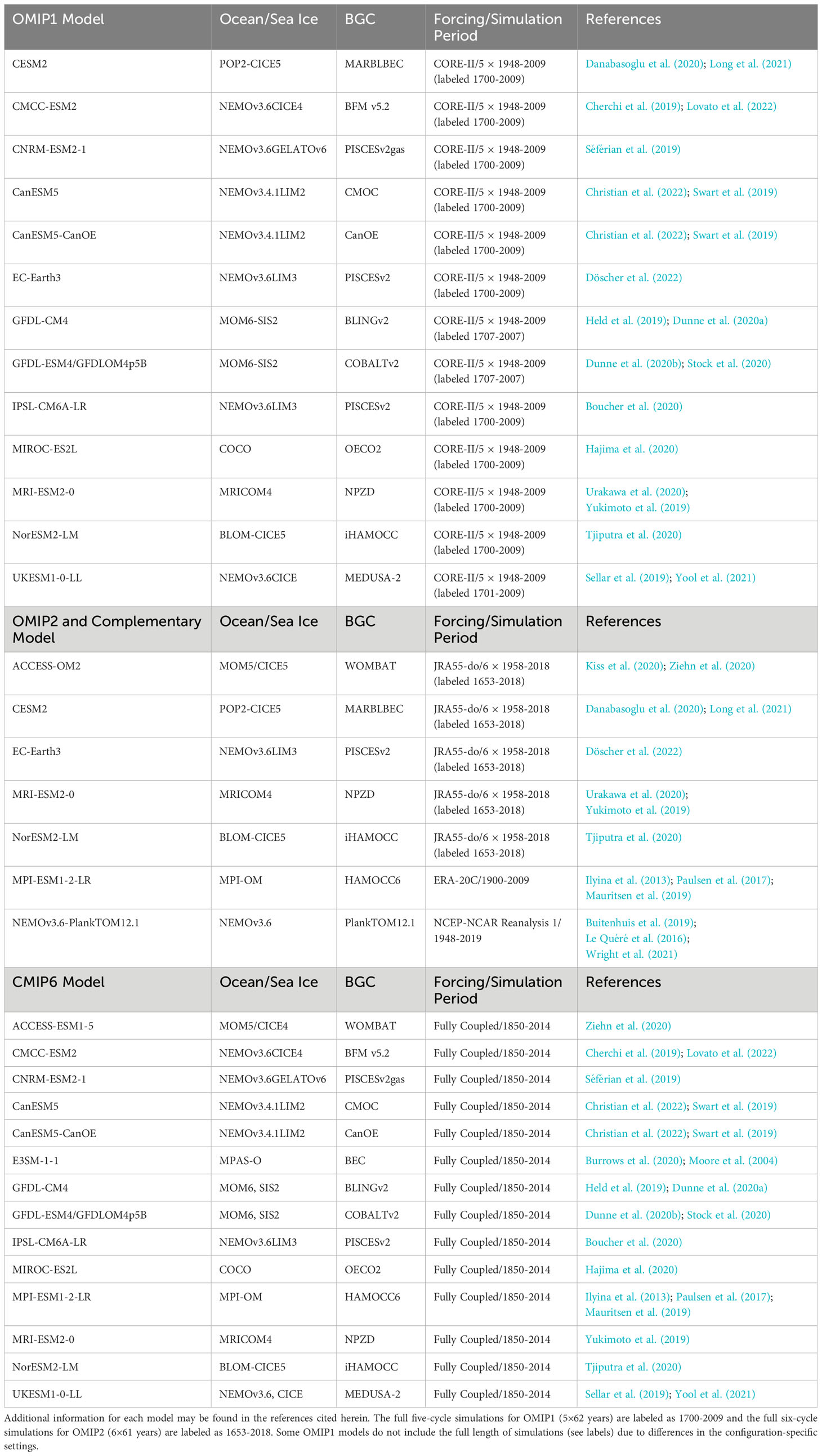
Table 1 The OMIP1, OMIP2, and CMIP6 Historical simulations used in this study, including the ocean, sea-ice, and biogeochemical model components, atmospheric forcing dataset, and simulation periods.

Our focus is mainly on the past 5 decades from 1960s to 2010s. This corresponds to the last cycle from the OMIP1 and OMIP2 simulations. We also analyzed two additional forced ocean-only model simulations to complement the analysis of OMIP simulations. One is based on the ECMWF ERA-20C atmospheric reanalysis forcing 1900-2009 for the MPI-ESM1.2 model, the ocean model MPI-OM with an ocean biogeochemistry model HAMOCC6 (Ilyina et al., 2013; Paulsen et al., 2017; Mauritsen et al., 2019), and the other is based on the NCEP-NCAR Reanalysis 1 atmospheric forcing (1948-2019) for the NEMOv3.6-PlankTOM12.1 (Le Quéré et al., 2016; Buitenhuis et al., 2019; Wright et al., 2021) from the University of East Anglia. The MPI-ESM1.2 model simulation is similar to the experimental design of the ocean carbon cycle simulation in the Global Carbon Budget project (Friedlingstein et al., 2019). The model was spun-up for millennia using the ECMWF ERA-20C atmospheric forcing from the early period (1900-1915) to achieve steady ocean states. An ocean simulation was then completed for the twentieth century using the ECMWF ERA-20C atmospheric forcing up to 2009. The NEMOv3.6-PlankTOM12.1 model was integrated from 1750-1947 (198 years) based on the NCEP-NCAR Reanalysis 1 climatological (a 1948-1977 daily climatology) atmospheric forcing followed by 61 years of hindcast simulation using the interannual atmospheric forcing from 1948-2009. Further details of these two additional simulations are provided in the Supplementary Material.

While the analysis periods differ slightly among the models and configurations, these differences were not found to significantly impact our results. We compare these simulations with the most recent and publicly available observational O₂ dataset (Ito, 2022). Before focusing on the analysis of model outputs from the recent decades, we briefly examine the models’ equilibrium states of upper ocean temperature and O₂ from OMIP1 and OMIP2 using the model output from the full length of the simulation cycles.

The CMIP6 Historical simulations (Eyring et al., 2016) are based on atmosphere-ocean-land coupled models listed in Table 1. The historical simulations span from 1850-2014 following the pre-industrial control simulations for each model. Duration of pre-industrial control simulations diverge among the models (e.g. Séférian et al., 2016; Séférian et al., 2020), but most of the CMIP6 models with ocean biogeochemistry have been spun-up longer than the standard OMIP protocol duration (except for the GFDL-CM4, which is a relatively highresolution ocean model). In the CMIP6 Historical simulations, the models are driven by the historical forcing (i.e. boundary conditions) of greenhouse gas concentrations, stratospheric and tropospheric aerosols, and land-use (Eyring et al., 2016). A comprehensive evaluation of ocean biogeochemical historical simulations based on CMIP6 models is documented in (Séférian et al., 2020). We analyze the model output for the past 5 decades from 1965-2014 to overlap with the observational dataset period.

2.2 Observational dataset

The observational product used in this study is the global three-dimensional, time varying O₂ dataset based on the quality-control bottle O₂ data from the World Ocean Database 2018 (WOD2018) from 1965-2015 (Ito, 2022) (hereafter ITO2022 dataset). This product is a 1-degree gridded product based on the optimal interpolation method to fill in spatial gaps. In this dataset, the number of O₂ samples is denser in 1970s and 80s, with more samples in the North Pacific and North Atlantic Oceans. The global coverage of samples is more even after 1990s, but overall, the samples remain relatively sparse, particularly after the year 2000 (see Figure 1 from Ito, 2022). Despite the interpolation, smoothing and gap filling procedures, the signals could be skewed towards the data dense regions in certain periods. Note that this product differs from the previous product (Ito et al., 2017), which includes Conductivity Temperature Depth (CTD) profiler measurements. The O₂ data product from ITO2022 dataset is presented as an anomaly relative to the long-term (1965-2015) mean (Ito, 2022), where O₂ concentrations are shown as yearly anomalies calculated using a 5-year moving averaging window. Note that a 5-year moving averaging window reduces the variability on timescales shorter than 5 years (Ito, 2022). The estimate of global ocean deoxygenation from this latest observational product is smaller than the previous works (Ito et al., 2017; Schmidtko et al., 2017) and thus provides a lower bound estimate of global ocean deoxygenation (Ito, 2022).

Figure 1

Figure 1 Time series of upper ocean global (0-700m) mean sea water temperature (A, E) and O₂ (C, G) from the OMIP1 and OMIP2 simulations from full cycles (310-366 years). OMIP-MM-MEAN is multi-model mean from both OMIP1 and OMIP2 simulations. Gray vertical dashed lines show the repeating forcing cycle, 5 cycles for OMIP1 and 6 cycles for OMIP2 simulations. The OMIP drift is defined as the difference between the initial condition and the historical climatology based on 50-year mean from the final cycle of the simulations to quantify the direction of model’s drift relative to the initial condition (B, D, F, H). Black horizontal dashed lines show zero lines.

We compare the upper ocean heat content (OHC) based on five dataset products to the simulated OHC from OMIP1, OMIP2, and CMIP6 configurations. These dataset products include the ECMWF Ocean Reanalysis System 4 (ORAS4) (following the previous observational O₂ and OHC study from Ito et al., 2017), EN4.2.1 from UK Met Office, Cheng dataset from the Institute of Atmospheric Physics (IAP), Chinese Academy of Sciences (http://www.ocean.iap.ac.cn/), Ishii dataset from Japan Meteorological Agency, and Levitus data from NOAA NCEI (Gouretski and Reseghetti, 2010; Levitus et al., 2012; Balmaseda et al., 2013; Ishii et al., 2017; Cheng et al., 2022). We additionally use the sea water temperature and salinity data from the ECMWF ORAS4, EN4.2.1, Cheng, and Ishii datasets to calculate oxygen saturation (O_2,satand Apparent Oxygen Utilization (AOU) (in sections 2.3 and 3.4). For climatological comparison of upper ocean O₂ (in section 3.1), we use the observations-based climatology from the World Ocean Atlas 2018 (Garcia et al., 2019).

2.3 Data analysis

To further examine the drivers of O₂ changes in the simulations and observations, we decomposed the O₂ changes into changes in O₂ saturation, i.e. the “thermodynamic” component, and changes in Apparent Oxygen Utilization (AOU), the component driven by changes in ocean circulation and biological activities (e.g. Emerson and Hamme, 2022). We first calculate O₂ saturation based on the Garcia and Gordon formula (Garcia and Gordon, 1992) and subtract the in-situ O₂ concentration to obtain AOU as follows:

$\begin{array}{ll}AOU=O_{2,sat}-O_2& (1)\end{array}$

which can be re-arranged to,

$\begin{array}{ll}{O}_2=O_{2,sat}-AOU& (2)\end{array}$

This decomposition is commonly used (e.g. Bopp et al., 2017) to highlight the thermal vs. non-thermal, circulation and biology driven O₂ changes in the ocean. In this study, we present -1 × AOU in figures to reflect more clearly its contribution to changes in O₂ (i.e. an increase in AOU is shown as a decrease in -1 × AOU, which translates to a decrease in O₂) (section 3.4).

All the model outputs are re-gridded to a 1-by-1 degree horizontal grid using distance weighted average remapping method (climate data operators (CDO); remapdis) (Schulzweida, 2022). The vertical interpolation is based on linear level interpolation (climate data operators (CDO); intlevel) (Schulzweida, 2022), interpolated from the model native levels to 102 vertical levels following the observational product, though our analysis focuses primary on the upper depth range (0-700m) of the ocean (i.e. the top 41 vertical levels). The spatial resolution of the re-gridded model output is the same as the ITO2022 dataset used in this study (Section 2.2). The main diagnostics of ocean deoxygenation and associated ocean warming for the past 5 decades are based on the anomaly of O₂ and sea water temperature relative to the long-term mean (i.e. the past 5 decades). The calculations of the anomaly of O₂ from the model output basically follows the ITO2022 dataset. We focus on upper ocean O₂ and heat content changes as this is where the majority of ocean physical and biogeochemical changes due to atmospheric forcing on inter-annual to decadal timescales are expected. Also the upper ocean environmental changes are highly relevant for marine ecosystems (e.g. Longhurst and Harrison, 1989). We calculate globally integrated O₂ inventory anomaly and OHC time series for comparing models and observations evaluations. OHC is in anomaly by definition (e.g. Levitus et al., 2012).

Ocean biogeochemistry simulations require a long term spin-up to reach equilibrium and can exhibit a long-term drift in their solution (Séférian et al., 2016). The standard OMIP protocols request 310-366 years for a model spin-up (Griffies et al., 2016), which is not sufficient for the deep ocean to achieve equilibrium state (e.g. Yool et al., 2020). The estimation of deep North Pacific Ocean ventilation age based on radiocarbon and inverse models is 1200-1500 years (Gebbie and Huybers, 2012; Khatiwala et al., 2012) or even longer timescales from some modeling studies (Wunsch and Heimbach, 2008). Unlike in the coupled model simulations, the OMIP1 and OMIP2 simulations have no control simulations to compare, making it important to assess the potential drift in OMIP simulations to ensure that it does not obscure the multi-decadal ocean deoxygenation signals in which we are interested. To check the impact of model’s spin-up in the upper ocean, the model’s equilibrium states of the sea water temperature and upper ocean O₂ are presented in the first part of the results following the ocean model intercomparison study by Tsujino et al., 2020.

To assess the models’ drift from forced ocean-only model simulations, we explore upper ocean global mean (covering 89.5°S-65°N in this study following the spatial coverage of the ITO2022 dataset) properties as a metric to evaluate the models’ equilibrium states for the variables on which we are focusing. Specifically we examine the global volume-weighted mean sea water temperature and O₂ from 0-700m from the OMIP1 and OMIP2 simulations (Figure 1). The time series of the global volume-weighted mean O₂ and sea water temperature from the upper ocean for the full cycles show individual model transitions to their respective quasi-equilibrium states for both properties. We show that for the final 50-60 years of the simulations, the analysis of ocean deoxygenation during this period is not significantly impacted by model drift in the upper ocean (see Figure 1).

We used linear trend analysis to quantify multidecadal changes in upper ocean O₂ inventory and OHC. Linear trend analysis is based on annual model output and observational dataset. The statistical significance test uses a modified Mann-Kendall test, which takes into account autocorrelations within the dataset (Yue and Wang, 2004; Hussain and Mahmud, 2019; Martínez-Moreno et al., 2021).

3 Results

3.1 Model solutions: equilibrium states of forced ocean simulations and climatological mean states

For the evaluation of models’ equilibrium states, we use the term “quasi-equilibrium states” to denote the upper ocean (0-700m) variables close to steady-states. For the OMIP1 simulations, most of the models reach quasi-equilibrium states in the fourth cycle (Figure 1), with approximately half of the models showing a positive drift anomaly in O₂ compared to the initial conditions based on the World Ocean Atlas 2013, though we expect the ocean to loose O₂ as the ocean warms. The positive drift anomaly in O₂ is likely driven by changes in ocean circulation and biological processes, offsetting the solubility-driven changes (see Supplementary Figure 1). Many of the models drift towards warm ocean states relative to the initial conditions except for the CNRM-ESM2-1, GFDL-CM4, and IPSL-CM6A-LR, from the OMIP1 and EC-Earth3 from the OMIP2 simulations. Three of these models (i.e. CNRM-ESM2-1, EC-Earth3, and IPSL-CM6A-LR) are based on the same ocean general circulation model, the Nucleus for European Modelling of the Ocean (NEMO) but the CNRM-ESM2-1 employs a different sea-ice model.

Despite differences in the atmospheric forcing between the configurations, the OMIP2 simulations exhibit a similar transition phase to the OMIP1 simulations, with most of the models reaching quasi-equilibrium states in the fourth cycle of the simulations. The EC-Earth3, for instance, runs under both OMIP1 and OMIP2 protocols, and its global mean O₂ equilibrates similarly in both simulations. The cyclically forced ocean-only model simulations also have issues involving the initial shock due to a jump in atmospheric forcing from the end to the beginning of the forcing period (Tsujino et al., 2020). Therefore, we omitted the first 10 years of the last cycle of the OMIP simulations from the analysis in Section 3.2.

Overall, the OMIP simulations shown here reach quasi-equilibrium states for both upper ocean O₂ and sea water temperature, and thus model drift does not substantially obscure the long-term trend associated with multi-decadal ocean deoxygenation due to global warming. We note, however, the timescales of the upper ocean quantities reaching quasi-equilibrium states are also model-dependent (e.g. Danabasoglu et al., 2014). Therefore, in some models, model drift could still impact detection of long-term changes (Tjiputra et al., 2023). Hereafter, we focus our analysis on the historical period after 1950s, which is represented by the last cycle from OMIP1 (1958-2009) and OMIP2 (1968-2018) simulations.

Next we compare the modern climatological mean states of upper ocean O₂ inventory from the OMIP1, OMIP2, and CMIP6 Historical simulations to the World Ocean Atlas 2018 (Garcia et al., 2019). Here we evaluate the upper ocean O₂ inventory, shown as maps of vertically integrated O₂ for each grid points from 0-700m (i.e refer to herein as column O₂ inventory) for the historical period. The modern climatological mean states are defined as the long-term mean of upper ocean column O₂ inventory 1958-2007 for the OMIP1 multi-model mean, 1969-2018 for the OMIP2 multi-model mean, and 1965-2014 for the CMIP6 Historical multi-model mean (Figure 2). The annual climatology from the World Ocean Atlas 2018 is based on measurements from the past 5 decades. We present here the multi-model ensemble mean from the OMIP1, OMIP2, and CMIP6 Historical simulations to summarize the characteristics of modern climatological column O₂ inventory from each configuration. For brevity, climatology of column O₂ inventory from the individual models are presented in the Supplementary Material.

Figure 2

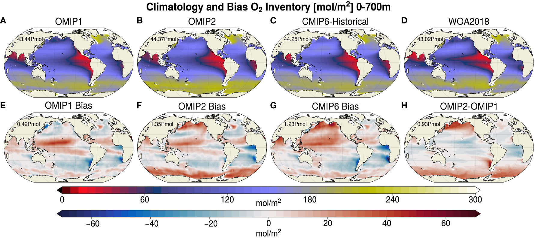
Figure 2 Climatological mean distributions of the upper ocean (0-700m) column O₂ inventory based on the past 5 decades of data. Column O₂ inventory is vertically integrated O₂ for each grid point. (A) OMIP1 multi-model mean, (B) OMIP2 multi-model mean, (C) CMIP6 Historical multi-model mean, and (D) from the World Ocean Atlas 2018. The number on upper left of each panel represents the globally integrated O₂ inventory. Lower (E–G) show difference between simulations and the World Ocean Atlas 2018. The (H) shows the difference between OMIP1 and OMIP2 multi-model mean [(B) minus (A)].

Overall the observed global patterns of modern climatological mean state of upper ocean column O₂ inventory are relatively well reproduced by the simulations, though biases emerge in key regions. The upper section (0-700m) of the oxygen minimum zone (OMZ) of the tropical Pacific Ocean, for instance, extend less westward than the observations and are simulated as a single spatially merged structure rather than two asymmetric northern and southern OMZs as shown in the World Ocean Atlas 2018 (Figure 2). Similarly, the OMZ in the tropical Atlantic Ocean is too intense in models, while the simulated Indian Ocean OMZ is weak (i.e. more O₂) compared to the observations. These biases were previously identified in CMIP5 model simulations (e.g. Cabré et al., 2015) and in CMIP6 model simulations in the Pacific OMZs (e.g. Busecke et al., 2022), and thus are shown to persist across CMIP effort. As Cabré et al., 2015 pointed out from analyzing CMIP5 models, the OMZ biases could stem from a deficient ventilation in the upper ocean, combined with a biologically driven downward flux of particulate organic carbon that is too large, resulting in a remineralization bias in these regions.

An additional mismatch between models and observations is the O₂ excess in the subpolar gyre region of the North Pacific Ocean. The World Ocean Atlas 2018 shows a deficit of O₂ in this region, but the models tend to have too much O₂ in this region for OMIP2 and CMIP6 Historical simulations. This is also a region where the model representations of climatological O₂ diverge substantially likely due to biases associated with poorly simulated ventilation processes (see Supplementary Material, Figures S3-S5). The globally integrated climatological upper ocean O₂ inventory (Figure 2) is slightly overestimated in the simulations (+0.42-1.35 Pmol) compared to the observational estimate of 43.02 Pmol. This overestimation stems from excess O₂ in the Southern Ocean and the western tropical Pacific Ocean in models compared to the observational estimate that overcompensate for the lower O₂ inventory of the eastern tropical Pacific Ocean and the tropical Atlantic Ocean (see Supplementary Material for further information).

The difference between OMIP1 and OMIP2 simulations shows how differences in the atmospheric forcing impact the climatology (i.e. quasi-equilibrium states) in O₂ (Figure 2H). The climatology of O₂ inventory from OMIP2 simulations show a higher O₂ in the North Pacific and the Southern Ocean indicating this updated atmospheric forcing results in more upper ocean O₂ inventory in these regions. Atmospheric wind impacts ventilation and mixing, and is expected to modulate O₂ and other ocean biogeochemical tracer variability and distributions. Previous work has also shown that biases in the atmospheric wind forcing in OMIP simulations project onto ocean circulations and water mass formation [e.g. in the tropical Pacific Ocean (Tseng et al., 2016)], with cascading effects on ocean biogeochemistry.

3.2 Global historical ocean deoxygenation and heat uptake: globally integrated changes

We examine the long-term trends and variability in O₂ inventory and OHC over the upper ocean global from the OMIP1, OMIP2, and CMIP6 Historical simulations (Figure 3). A prominent feature for the OMIP1 models - based on the CORE-II atmospheric forcing (Large and Yeager, 2009) - is an initial decrease in the upper ocean O₂ inventory through the mid 1980’s followed by an increase in the remaining 25 years of the simulation (Figure 3A). This increase is in contrast to the long-term decrease reported in recent observational studies (Helm et al., 2011; Ito et al., 2017; Schmidtko et al., 2017; Ito, 2022). The shift from a decadal decrease to an increase in the upper ocean O₂ inventory during the mid 1980’s coincides with the El Chichón and Pinatubo eruptions which have been proposed to drive a multi-year increase in the upper ocean O₂ inventory through cooling of the ocean and intrusion of O₂ (Eddebbar et al., 2019). The volcanic effects were previously assessed in the large ensemble simulations (e.g. Eddebbar et al., 2019; Fay et al., 2023) and emerge similarly here in the CMIP6 Historical multi-model mean (see the Pinatubo-related pause in ocean deoxygenation and heat loss in CMIP6 Historical in Figures 3A, B), but this signal is challenging to detect in OMIP simulations and observations. The discrepancy in OMIP simulations could be due to the confounding effect of atmospheric driven climate variability (i.e. such as a common wind forcing in OMIP simulations modulating the ocean circulation) or OMIP simulations are less sensitive to volcanic effects. Detection of volcanic effect in observations is particularly challenging given the large gaps and uncertainties in the dataset. The complementary MPI-ESM1.2 simulation - based on the ECMWF ERA-20C atmospheric forcing (Poli et al., 2016) - also shows a slight increase in O₂ inventory. While the OMIP1 simulations show a net uptake in heat as expected from anthropogenic forcing, the overall ocean heat uptake is weak, with many models showing little to no heat uptake in the first decades of the simulation (see Supplementary Material, Figures S6 and S7), potentially explaining the weak negative O₂ trends. All OMIP1 simulations and complementary simulations however show an increase in heat uptake in the recent decade (1995-2008), which is initially unexpected given the coincident increase in O₂ during this period.

Figure 3

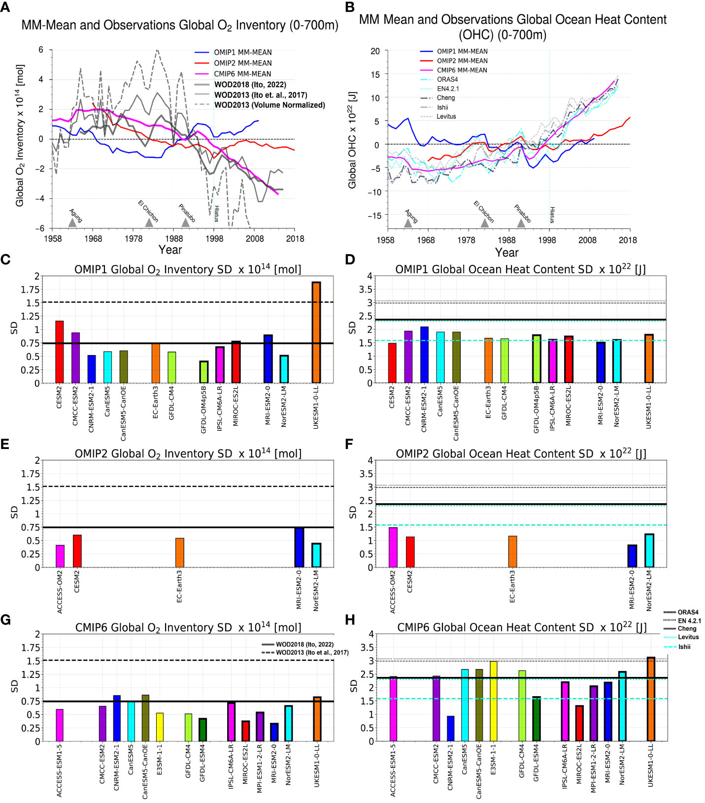
Figure 3 Historical time series of upper ocean (0-700m) global O₂ inventory anomaly and ocean heat content (OHC) from OMIP1, OMIP2 and CMIP6 Historical multi-model mean and observational dataset for (A, B). Note that time series for OMIP2 simulations from 1958-1967 are omitted from the analysis because of the initial forcing shock from the repeat forcing applied to the models (Tsujino et al., 2020). The reference for the anomaly for each simulation is, 1958-2007 for the OMIP1, 1969-2018 for the OMIP2, and 1965-2014 for the CMIP6 Historical simulations, respectively. Gray triangles denote the timing of major volcanic eruptions and vertical cyan lines denote the timing of “hiatus”. (C–H) show the summary of temporal SD (i.e. variability) of global O₂ inventory and OHC from the OMIP1, OMIP2 and CMIP6 Historical simulations. Temporal SD is based on SD from the past 50 years (the same as the reference periods) of detrended global O₂ inventory and OHC time series. Temporal SD from the observational datasets are shown in horizontal lines (black and cyan solid and dotted lines).

In contrast, the OMIP2 simulations, which are based on the JRA55-do atmospheric forcing (Tsujino et al., 2018), show a decrease in the upper ocean global O₂ inventory since the beginning of the time series (i.e. at year 1968), though the rate of O₂ loss is much weaker compared to observations (Figure 3A). The decadal shift in the O₂ inventory in the OMIP2 simulations from a long-term decrease to a brief increase and subsequent flattening is centered around the end of the 1990’s and independent from the timing of the volcanic eruptions of El Chichon´ and Pinatubo. The ocean overall takes up more heat in the OMIP2 than the OMIP1 simulations, though heat uptake is still weaker compared to the observations (Figure 3B). In the OMIP2 simulations, the ocean continues to take up heat after 2000 (“hiatus decade”) while the oceanic O₂ inventory remains relatively unchanged (Figures 3A, B), suggesting a potential decoupling of the changes in heat and O₂ contents during these recent decades. We also note a much stronger agreement across the OMIP2 models for both O₂ inventory and OHC changes than in the OMIP1 models (see Supplementary Material, Figures S6, S7). More than half of the models (8 out of total 13 models) from OMIP1 simulations show positive trend in the O₂ inventory (and all the models show a negative OHC trend, which is counter-intuitive), whereas all the models from OMIP2 simulations show a negative trend in O₂ inventory. We note, however, that there are fewer simulations of OMIP2 compared to OMIP1 simulations.

Compared to the OMIP simulations, the CMIP6 Historical simulations show a substantial decrease in the O₂ inventory over the past 50 years (Figure 3A), in line with the most recent observational estimate of Ito (2022) likely due to warming of the ocean and reduction in ventilation supply. The signature of the major volcanic eruptions are also pronounced in these simulations (Figures 3A, B, particularly for Agung (1963-1965) and Pinatubo (1991-1994), in line with the expected cooling of the upper ocean (Figure 3B) and intrusion of O₂ following eruptions which acts to temporarily slow down the advance of ocean deoxygenation (Eddebbar et al., 2019; Fay et al., 2023). The O₂ loss shown by the CMIP6 Historical simulations occurs alongside significant heat uptake which is also in line with the observed estimate of changes in the upper OHC (Figure 3B).

Simulated O₂ shows weaker variability than observed at depth (Long et al., 2016), an issue that likely persists in the OMIP and CMIP6 simulations (Figures 3C, E, G). About half of the models show lower temporal SD in global O₂ inventory compared to the latest ITO2022 dataset (magnitude ∼ 0.75 × 10¹⁴ mol) and much smaller than the temporal SD from the previous dataset from Ito et al., 2017 (Figures 3C, E, G). While the CMIP6 Historical simulations show a relatively strong 50-year downward trend (Table 2) in the global O₂ inventory, major biases associated with physical and biogeochemical processes (e.g. zonal equatorial currents and eddies) in hinders their ability to reproduce observed variability of O₂ (e.g. Busecke et al., 2019). The temporal SD of global OHC time series from OMIP1 and OMIP2 simulations are smaller compared to the CMIP6 Historical simulations. Compared to the recent observational OHC time series, the simulated temporal SD might underestimate the observed fluctuations compared to the temporal SD from the Cheng and Levitus datasets. The ECMWF ORAS4 and EN4.2.1 show higher SD compared to the simulations and other observational datasets.

Table 2

Table 2 Multi-decadal linear trend of upper ocean global O₂ inventory and OHC.

The 50-year linear trend in upper ocean global O₂ inventory and OHC for models and observations are summarized in Table 2. The magnitude of the total decrease of global O₂ inventory over the historical simulation period is about 4−5×10¹⁴ [mol] for the CMIP6 Historical simulations (Figure 3A and Supplementary Material), which is much stronger than the OMIP simulations. The latest estimates based on observational dataset shows a similar range, though discrepancies between observational products arising from gaps in observational coverage and differences in interpolation methods continue to generate large uncertainties in the rate of global ocean deoxygenation (Ito, 2022). A detailed observations-model comparison requires sub-sampling, gridding, and interpolation of model outputs in similar fashion to the observational estimates and will be addressed in a separate study (Ito et al., 2023).

Because ocean deoxygenation is driven by warming, we expect global O₂ inventory loss during periods of increased OHC, which is reflected in the observations-based products (Ito et al., 2017). The changes in OHC in the OMIP1, OMIP2 and CMIP6 Historical simulations do show heat gain in the upper ocean, although heat uptake in the OMIP simulations is substantially weaker compared to the CMIP6 Historical simulations (Figure 3B). This is likely due to adjustment of the ocean models to specific atmospheric forcing (Large and Yeager, 2009) and model spin-up procedures (e.g. simulations from Berthet et al., 2023 also showed an improvement representing observed upper 300m OHC using a modified OMIP2 protocol). To summarize, despite their shortcomings in representing the trends of ocean O₂ loss and heat uptake, the OMIP2 simulations show a general improvement in representing global ocean deoxygenation compared to the OMIP1 simulations, a feature that is likely due to improved representation of the atmospheric forcing such as wind (Taboada et al., 2019) and precipitation fields used to spin-up and run the ocean models.

3.3 Global historical ocean deoxygenation and heat uptake: spatial and vertical patterns

The linear trend patterns from the OMIP and CMIP6 Historical simulations show substantial differences among the configurations both in magnitudes and even sign of O₂ changes (Figure 4). The linear trend of column O₂ inventory in OMIP1 simulation is generally large and shows both positive and negative trends in different regions of the world ocean (Figure 4A). The positive column O₂ trend patterns in OMIP1 are pronounced in the subtropical North Pacific Ocean and in the high latitude Southern Ocean. Another key OMIP1 feature is that warming and cooling in the Pacific Ocean leads to a gain and loss of O₂, respectively, was initially counter intuitive and is likely due to ocean circulation and biological processes rather than solubility driven changes (see section 3.4 for further discussion). The OMIP2 and CMIP6 Historical simulations overall show weaker magnitudes in linear trend than OMIP1 for both column O₂ inventory and OHC. The CMIP6 Historical simulations show an overall loss of O₂ that is well distributed globally, with intense regions of ocean deoxygenation focused in the North Atlantic, North Pacific and Indian Ocean that are tightly associated with ocean warming in these regions. The warming of the Southern Ocean, however, shows relatively little changes in the column O₂ inventory in CMIP6 Historical simulations.

Figure 4

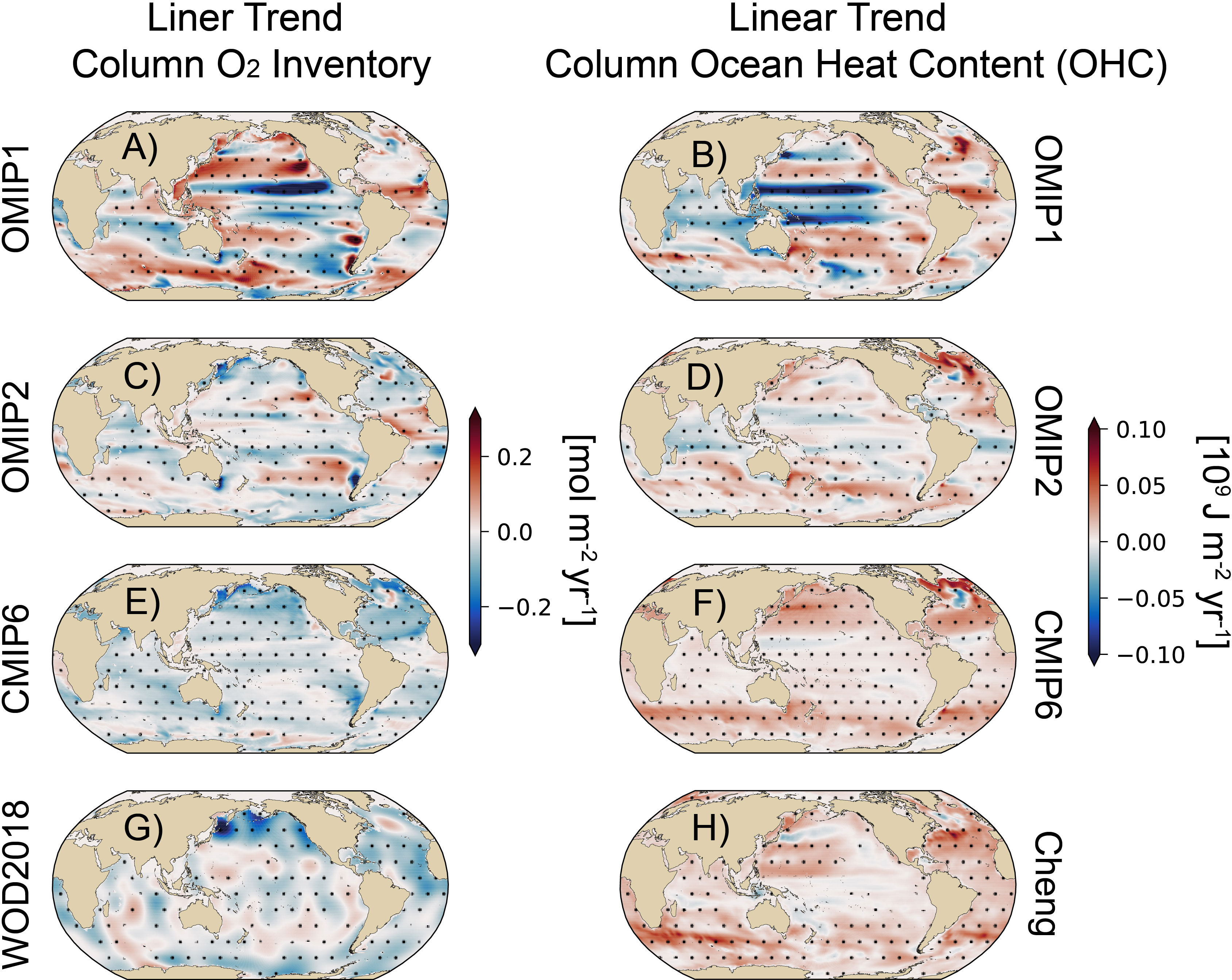
Figure 4 Patterns of linear trend of upper ocean (0-700m) column O2 inventory and OHC for the past 5 decades from models and observation. Model simulations are based on multi-model mean from each configuration. Linear trend calculation period for each simulation is, 1958-2007 for the OMIP1 (A, B), 1969-2018 for the OMIP2 (C, D), and 1965-2014 for the CMIP6 Historical simulations (E, F). The regions with black dots show locations of trend statistically significant above the 95% confidence level based on a modified Mann-Kendall test. The observational column O2 inventory and OHC are from WOD2018 (Ito, 2022) and Cheng’s dataset (Cheng et al., 2022) (G, H). The OHC trend from other observational dataset are in Supplementary Material.

The OMIP simulations are driven by atmospheric reanalysis-based forcing which includes both an atmospheric internal climate variability component and an externally generated forced response (e.g. greenhouse gases, volcanic and anthropogenic aerosols), and thus the ocean signature (shown by the OMIP means) of the atmospheric driven internal climate modes and anthropogenic drivers is common across model simulations. The CMIP6 Historical simulations, however, generate their own internal climate variability in the coupled climate system from each model ensemble member (e.g. Deser et al., 2020), and thus the CMIP6 multi-model mean largely highlights the ocean response to external forcing (i.e. global warming), as the internal climate variability component is presumably smoothed over in the multi-model mean. As a result, a more homogeneous pattern emerges in the CMIP6 Historical simulations that mainly reflects the anthropogenic responses (i.e. ocean deoxygenation and warming) while the OMIP models contain signatures associated with the specified atmospheric forcing (Figures 4E, F).

The observational patterns show a less uniform distribution than the CMIP6 Historical simulation trends, likely due to the combined effects of internal climate variability and external forcing, though the limited observational coverage and gap filling methods may induce some of the patchy signals of upper ocean column O₂ inventory shown in Figure 4G. In the observational product, the North Pacific O₂ loss is pronounced, which is missing in OMIP simulations and only weakly simulated in CMIP6 Historical simulations. The tropical and subtropical regions show areas of positive O₂ trends, indicating that these regions may respond differently to anthropogenic forcing than the high latitudes, or that internal climate variability might play a more dominant role in these regions. An interesting feature that exists across simulations and observations is cooling (i.e. “warming hole”) in parts of the subpolar North Atlantic Ocean (e.g. Rahmstorf et al., 2015; Keil et al., 2020), that is associated with an increase in O₂. This cooling and O₂ increase is occurring along with broad ocean warming and deoxygenation in the North Atlantic, and likely reflects an ocean physical response to anthropogenic forcing (Rahmstorf et al., 2015; Keil et al., 2020).

The upper ocean vertical structures (i.e. Hovmo¨ller diagram of depth vs time) of global area-weighted mean O₂ and sea water temperature highlight how deep the ocean deoxygenation and warming signals penetrate into the ocean (Figures 5, 6). In all but the OMIP1 simulations, the ocean is losing O₂ and gaining heat at depth. The OMIP1 deoxygenation occurs mainly in the upper 200m, and increase in O₂ below 200m after 1995, which is consistent with their simulated increase in upper ocean global O₂ inventory in recent decades (Figure 3A). The OMIP2 simulations show a general decrease in O₂ throughout the upper ocean, though most of the O₂ loss occurs in the upper 200m. In contrast, the CMIP6 Historical simulation show a substantial decrease in global O₂ throughout the upper 700m associated with the anthropogenic warming effects, though the highest rates of O₂ loss are found between 200-600m depth, in line with reduced ventilation of the thermocline in a warming world (Keeling and Garcia, 2002). There are also contrasts in the vertical penetration of anthropogenic heat and O₂ loss, whereby the pronounced O₂ changes penetrate down to 700m but the largest heat uptake signal is in the upper 200m (Figures 5, 6), suggesting the large role of stratification and reduced ventilation in setting the O₂ changes at depth in the CMIP6 Historical simulations. This is evident from the changes in AOU (see section 3.4 and Supplementary Material) and likely the combined physical-biological effect supports O₂ loss penetration further down into the ocean compared to OHC.

Figure 5

Figure 5 Hovmöller diagram of upper ocean (0-700m) O2 anomaly from a suite of model simulations and observational dataset. The values depict the global area-weighted average of O2 anomaly for each depth. The anomaly is defined as a deviation from the reference long-term climatology. The reference for the anomaly for each simulation is, 1958-2007 for the OMIP1 (A), 1969-2018 for the OMIP2 (B), 1965-2014 for the CMIP6 Historical simulations (C), and for the World Ocean Database 2018 (Ito et al., 2022) (D), respectively. Model simulations are based on multi-model mean. Gray triangles denote the timing of major volcanic eruptions and vertical gray lines denote the timing of “hiatus”.

Figure 6

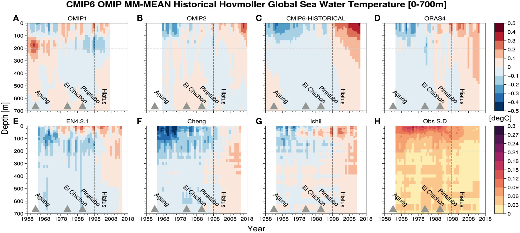
Figure 6 The same as in Figure 5, except for sea water temperature anomaly. The Hovmöller diagram of sea water temperature anomaly include results from the models (A–C) and four different observational datasets (D–G). Ensemble data spread (SD) for observational datasets is included in (H).

The observational vertical patterns show a relatively similar ocean deoxygenation response to the CMIP6 Historical simulations (Figure 5D), with O₂ signals penetrating down to 700m, suggesting that the observations may be reflecting changes associated largely with anthropogenic warming. Positive anomalies in O₂ are found at depth following eruptions, as expected from the effects of volcanic eruptions on the O₂ content (Eddebbar et al., 2019; Fay et al., 2023), though the observational product does not show a major anomaly associated with the Pinatubo eruption (Figure 5D), potentially due to the large anthropogenic forcing and internally generated variability effects during the later decades. The patchiness in O₂ anomalies found in observations and OMIP simulations are likely due to atmospheric or oceanic internal climate variability. Similarly to the globally integrated trend analysis discussed above, the warming and O₂ changes shown at depth in both OMIP simulations are weaker compared to the CMIP6 Historical simulations and observations, particularly for the OMIP1 simulations which show cooling around 200m depth. The observational changes in global OHC for upper ocean overall shows transition from cooling to warming in the upper few hundred meters, although Cheng’s dataset shows intense cooling from 1960s to 1970s compared to the other dataset (Figure 6).

3.4 Drivers of historical ocean deoxygenation: thermodynamics vs. circulation and biology

Global O₂ saturation decreases in OMIP2 and CMIP6 Historical simulations, but the magnitudes differ among the simulations (Figure 7 and Supplementary Material). The most intense O₂ saturation loss is found in the CMIP6 Historical simulations, consistent with the intense global ocean heat uptake in the upper ocean (Figure 3B). The OMIP1 simulations show weak or even no change in saturation driven O₂ changes. The complementary simulations (MPI-ESM1-2-LR and NEMOv3.6-PlankTOM12.1) show a much stronger decrease in O₂ saturation likely due to different model spin-up procedures in these simulations (see Supplementary Material). The dominant driver of global ocean deoxygenation is AOU, also a major source of uncertainty in simulating historical deoxygenation. The CMIP6 Historical simulations and observations show an increase in AOU (i.e. decrease in O₂), which reinforces the thermally driven O₂ loss (Figure 7 and Supplementary Material). The OMIP1 simulations show decrease in AOU, which is a major factor for the oxygenation in the last decades of these simulations.

Figure 7

Figure 7 Historical time series of upper ocean (0-700m) global mean O_2,satand -1 × AOU (see section 2.3) from OMIP1, OMIP2 and CMIP6 Historical multi-model mean and observational dataset (A, B). Note that time series for OMIP2 simulations from 1958-1967 are omitted from the analysis because of the initial forcing shock from the repeat forcing applied to the models (Tsujino et al., 2020). The reference for the anomaly for each simulation is, 1958-2007 for the OMIP1, 1969-2018 for the OMIP2, and 1965-2014 for the CMIP6 historical simulations. Gray triangles denote the timing of major volcanic eruptions and vertical cyan lines denote the timing of “hiatus”.

The spatial patterns of changes in upper ocean vertical mean O₂ saturation and AOU are shown through a map of linear trends over the past 50 years in Figure 8. Similar to the linear trend analysis of column O₂ inventory and OHC (Figure 4), the OMIP1 simulations show intense changes on multi-decadal timescales, and the magnitude of the trend is larger in AOU than O₂ saturation. The response in O₂ saturation in OMIP1 models is consistent with their weak OHC change in Figure 4, and thus AOU changes play a more important role in regions with deoxygenating (oxygenating) and cooling (warming) tendencies. Similarly, the O₂ saturation trends in the OMIP2 and CMIP6 Historical simulations and observations are weaker than the AOU trends, with AOU playing a key role in the tropical basins for the CMIP6 Historical simulations. The CMIP6 Historical simulations overall show a uniform decrease in O₂ saturation due to warming and increased AOU. This increase in AOU is likely due to reduced ventilation supply of O₂ from the surface into the interior ocean. The strong AOU increase in the North Pacific Ocean from observations may include contributions from the internal climate variability which is weak but is partly evident in the OMIP2 simulations. The North Atlantic warming hole signature is evident in the O₂ saturation changes, which is consistent with changes in OHC (Figure 4).

Figure 8

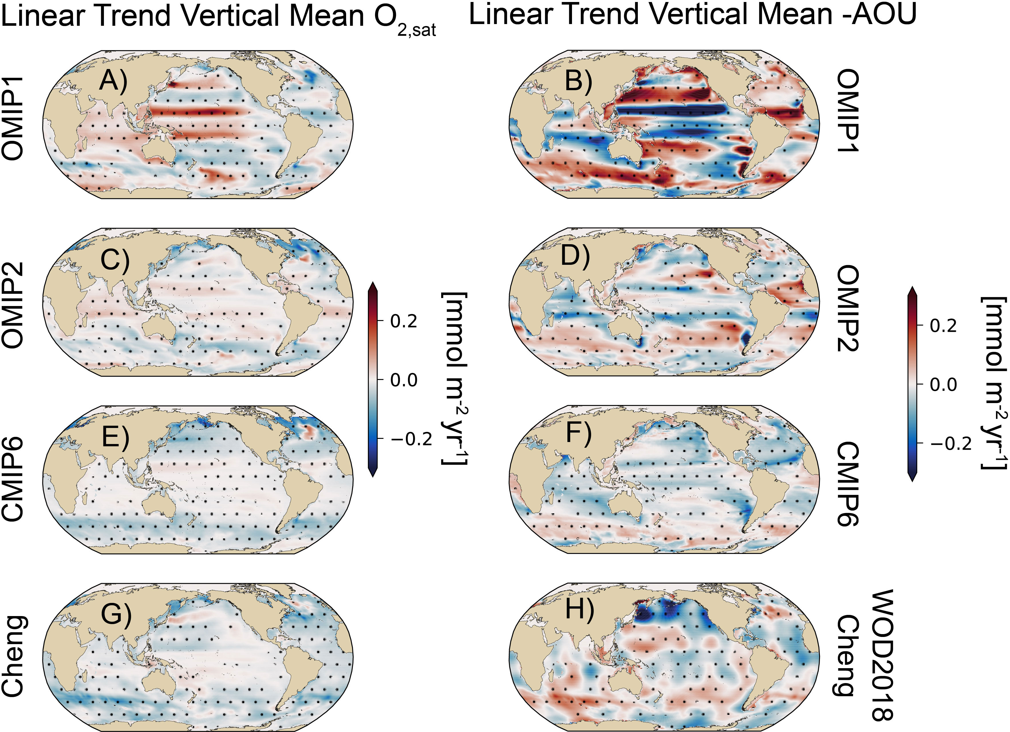
Figure 8 Linear trend of upper ocean (0-700m) vertical mean O2 saturation and -1 × AOU. Linear trend calculation period for each simulation is 1958-2007 for the OMIP1 (A, B), 1969-2018 for the OMIP2 (C, D), and 1965-2014 for the CMIP6 historical (E, F) simulations. The region with black dots show locations of trend statistically significant at the 95% confidence level based on a modified Mann-Kendall test. The observational O2 saturation and AOU are based on WOD2018 (Ito, 2022) and Cheng’s dataset (Cheng et al., 2022) (G, H). The O2 saturation and AOU from other observational datasets are in Supplementary Material.

The upper ocean vertical structures (i.e. Hovmöller diagram of depth vs time) of O₂ saturation and AOU highlight the drivers of ocean deoxygenation in the surface and interior ocean (see Supplementary Material). The simulations and observation both exhibit thermal loss of O₂ in upper 100m, but how deep the thermal loss penetrates differs among the configurations. The CMIP6 Historical simulations and observation are relatively similar in vertical structures of thermal loss, which penetrates down to 700m but OMIP simulations thermal loss is restricted to the top 200m. In OMIP1 simulations, there is an increase in O₂ saturation, likely driven by cooling at 200m depth.

To summarize the relationship and relative contributions of these two components, we present global changes in O₂ saturation and AOU for models and observations in the scatter plots shown in Figure 9. The global changes in O₂ saturation and AOU are based on global volume-weighted mean of these properties within the upper 700m of the ocean. The OMIP1 simulations show overall relatively weak changes in O₂ saturation ranging from -0.5 to 0.5 mmol m⁻³ compared to the wide spread changes in AOU from -1.5 to 1.0 mmol m⁻³ during the historical era, the latter likely explaining the positive shift in the global O₂ inventory and reduced O₂ loss in OMIP1 simulations. The OMIP2 simulations similarly show a narrow spread in O₂ saturation change along with narrower spread in AOU changes compared to the OMIP1 simulations, likely explaining the global O₂ inventory shifts towards negative values in the OMIP2 simulations. A major difference between model experiments is the strong changes in the CMIP6 Historical simulations towards negative O₂ saturation as much as -1 mmol m⁻³ and increasing AOU, which results in stronger ocean deoxygenation trends in these simulations, consistent with the trends shown in Figures 3, 4. The strong negative O₂ saturation and AOU changes are consistent with the intense simulated ocean heat uptake in CMIP6 Historical simulations, and observations (Figure 9, black lines and dots).

Figure 9

Figure 9 Relationship between upper ocean (0-700m) global O₂ saturation and -1 × AOU from a suite of model simulations and observational datasets. The O₂ saturation and minus AOU are in anomaly relative to long-term mean and scatter plots are based on the model output and observations from the past 5 decades [1958-2007 for OMIP1 multi-model mean (A), 1969-2018 for OMIP2 multi-model mean (B), and from 1965-2014 for CMIP6 Historical multi-model mean (C), and 1965-2015 for observations (A–C)]. Colored dots represent individual models and solid colored lines are linear regression between O₂ saturation and minus AOU from the multi-model mean. The label +O₂ in the first quadrant shows where gain in O₂ occurs due to changes in O₂ saturation and minus AOU (and similar for -O₂ in the third quadrant). Black dots and triangles represent the O₂ saturation and -1 × AOU based on observations (World Ocean Database 2018 (gridded dataset from Ito, 2022) for O₂ and four observational datasets for sea water temperature and salinity).

3.5 The O₂ to heat ratio: how tightly are global ocean deoxygenation and warming related?

The global O₂ inventory is known to be tightly and negatively correlated with global OHC in the upper ocean (Bopp et al., 2002; Keeling and Garcia, 2002; Ito et al., 2017). Here, we examine this global O₂ Heat relationship within the context of the historical era in the OMIP1, OMIP2, and CMIP6 Historical simulations and observations. A key feature in the OMIP1 simulations is the absence of a strong relationship between the global O₂ inventory and OHC in the multi-model mean, with a broad spread across individual models (gray dots and the blue line in Figure 10A). The OMIP2 simulations show a more negative and tighter relationship between the two properties (gray dots and the red line in Figure 10B), with narrower spread between models than the previous OMIP1 simulations. This is likely due to differences in theatmospheric forcing driving a more intense and sustained ocean deoxygenation and heat uptake. The CMIP6 Historical simulations show a tight relationship between the O₂ and heat contents (gray dots and the magenta line in Figure 10C), with a similar slope to the OMIP2 simulations (see Figures 10B, C). Table 3 summarizes the regression coefficients between global O₂ inventory and OHC. The regression coefficients from OMIP2 and CMIP6 Historical simulations (-3.2 and -2.8 [nmol/J]) are close to the observational values (-2.3 to -2.6 [nmol/J]) while the OMIP1 simulations show a weak relationship (-0.4 [nmol/J]) (Table 3). This indicates that the OMIP2 simulations capture the observed global O₂ - Heat relationship. This tighter global O₂ - Heat relationship compared to that of the OMIP1 simulations are likely due to improvements in the atmospheric forcing.

Figure 10

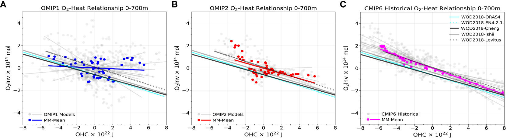
Figure 10 Relationship between upper ocean (0-700m) global O₂ inventory and OHC from a suite of model simulations and observational dataset from the past 5 decades (1958-2007 for OMIP1 (A), 1969-2018 for OMIP2 (B), and from 1965-2014 for CMIP6 Historical (C), and 1965-2015 for observations (included in A-C along with model simulations)). Gray dots represent individual models and solid colored dots are multi-model mean. The lines show linear regression between the global O₂ inventory and OHC.

Table 3

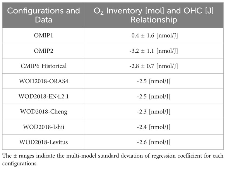
Table 3 A list of global O₂ inventory and OHC relationship presented as linear regression coefficients from the past 5 decades (1958-2007 for OMIP1 multi-model mean, 1969-2018 for OMIP2 multi-model mean, and from 1965-2014 for CMIP6 Historical multi-model mean, and 1965-2015 for observations) of time series from the models and observations.

Where do these differences in the simulated and observed global O₂ inventory and OHC relationships originate? To elucidate this, we show global correlation coefficient patterns of column OHC (i.e. twodimensional data) against the globally integrated upper ocean (0-700m) O₂ inventory time series (i.e. one-dimensional data) over the historical period (i.e. the past 5 decades) (Figure 11). This enables us to highlight in which region the ocean gains or loses heat when global O₂ inventory changes. For example, the positive correlation coefficient indicates that the increase in global O₂ inventory is associated with increase in column OHC in a specific region (grid points) (i.e. counter intuitive relationship). We note that the O₂ inventory and OHC data have not been de-trended in this analysis to focus more on the long-term changes and linear relationships. Key differences emerge in the correlation coefficient fields from the OMIP1 simulation, showing a positive relationship between O₂ inventory and OHC throughout the northern subpolar, subtropical, and tropical Pacific and North Atlantic basins, though with low agreement between models in the tropical Pacific Ocean. The positive relationship in these regions likely drives the weak global O₂ - Heat relationship shown in Figure 10A. These positive correlations are diminished in the North Atlantic and the Southern Ocean in the OMIP2 simulations, which results in improved global O₂ - Heat relationship (Figure 10B). The correlation pattern from CMIP6 Historical simulations show relatively uniform negative correlation coefficients similar to that of observations except that the signals in the mid to high latitude oceans are larger. The correlation pattern from CMIP6 Historical simulations are much more constrained possibly because of multi-model mean procedures highlighting signals of long-term, global warming trend.

Figure 11

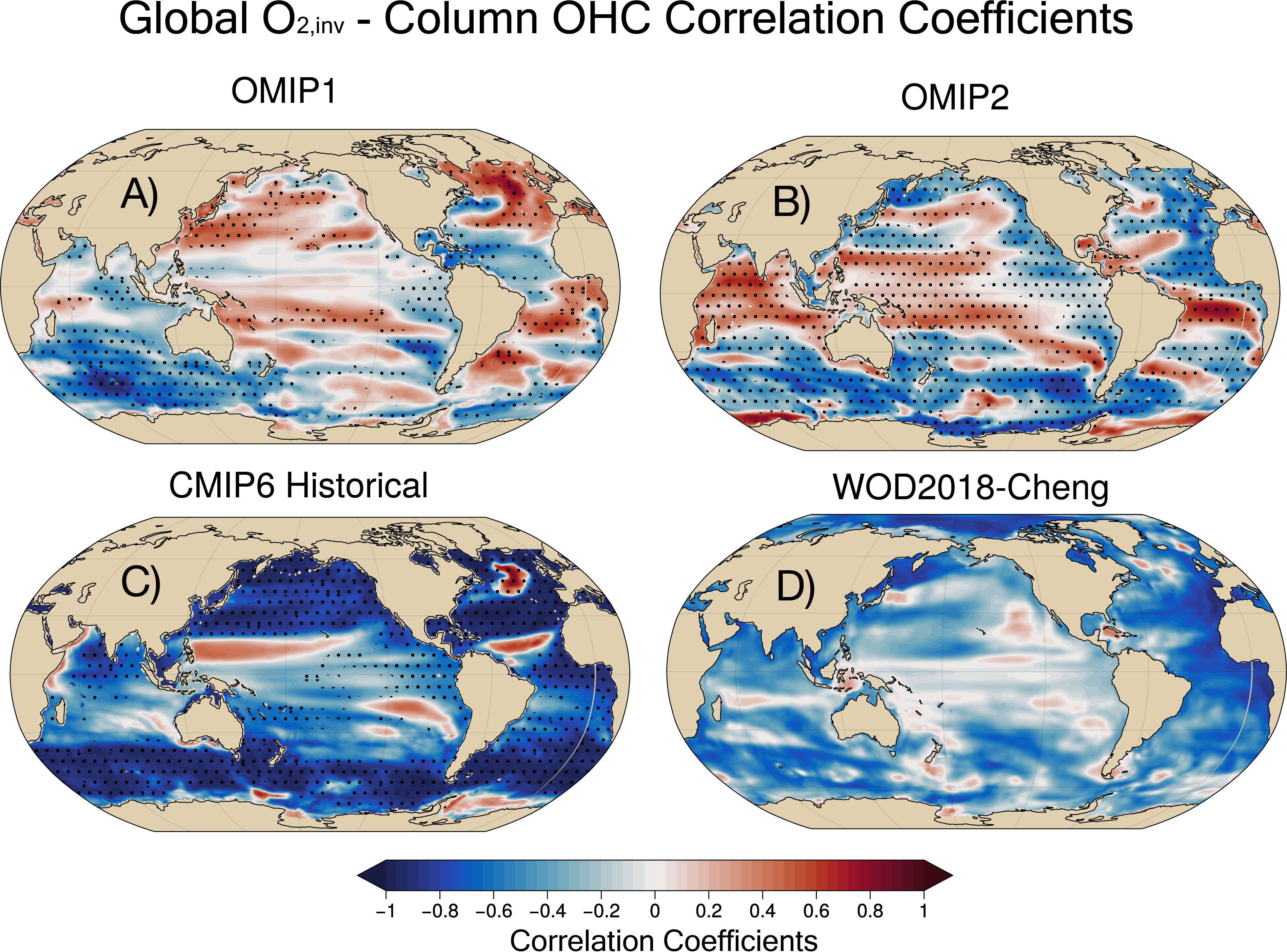
Figure 11 Correlation coefficient patterns of column OHC (i.e. two-dimensional data) against the globally integrated upper ocean O₂ inventory time series (i.e. one-dimensional data) averaged over all models (A–C) and from an observational dataset (D). No de-trending applied to the data to focus on the trend signals. Black dots designate robustness, as defined by at least 80%model sign agreement in correlation coefficients. The correlation analysis is based on the period of 1958-2007 for OMIP1, 1969-2018 for OMIP2, 1965-2014 for CMIP6 Historical, and 1965-2015 for the observations [WOD2018 and Cheng’s dataset (Cheng et al., 2022; Ito, 2022)]. Correlation coefficients based on other observational column OHC dataset are in Supplementary Material.

4 Discussion and conclusion

Through a comprehensive analysis of the OMIP and CMIP6 Historical simulations, we found that the simulations show substantial differences in the rate and spatial patterns of global O₂ inventory loss in the upper ocean over the historical era. These differences likely arise from differences in the ocean models background mean states set by the spin-up procedures as well as the atmospheric forcing product likely associated with adjustments to the surface wind and buoyancy forcing.

4.1 Potential impact of atmospheric forcing

Differences in the long-term trend of the surface wind stress fields between OMIP1 (CORE-II) and OMIP2 (JRA55-do) (in Figure 12) could lead to bias in spun-up states and subsequent decadal response in the upper ocean O₂ inventory. A spurious trend in zonal wind stress in the tropical Pacific Ocean (also discussed in Yeager et al., 2018; Ito et al., 2019 and see Figure 12A) likely leads to O₂ inventory and OHC biases in the Pacific Ocean (see Figure 4) through changes in the equatorial currents and upwelling in this region. These biases overall impact on the global O₂ inventory and OHC in the OMIP1 simulations. Therefore, while the OMIP1 simulations struggle to simulate the observed O₂ loss, OMIP2 simulations show improvement to some extent in simulating global ocean deoxygenation likely due to reduced bias in zonal wind stress and increased resolution of the wind fields (Oschlies et al., 2018; Taboada et al., 2019). We do note that the complementary simulations based on the ECMWF ERA-20C and the NCEP-NCAR Reanalysis 1 atmospheric forcing did not show much of a difference in O₂ inventory response even with a different spin-up procedures.

Figure 12

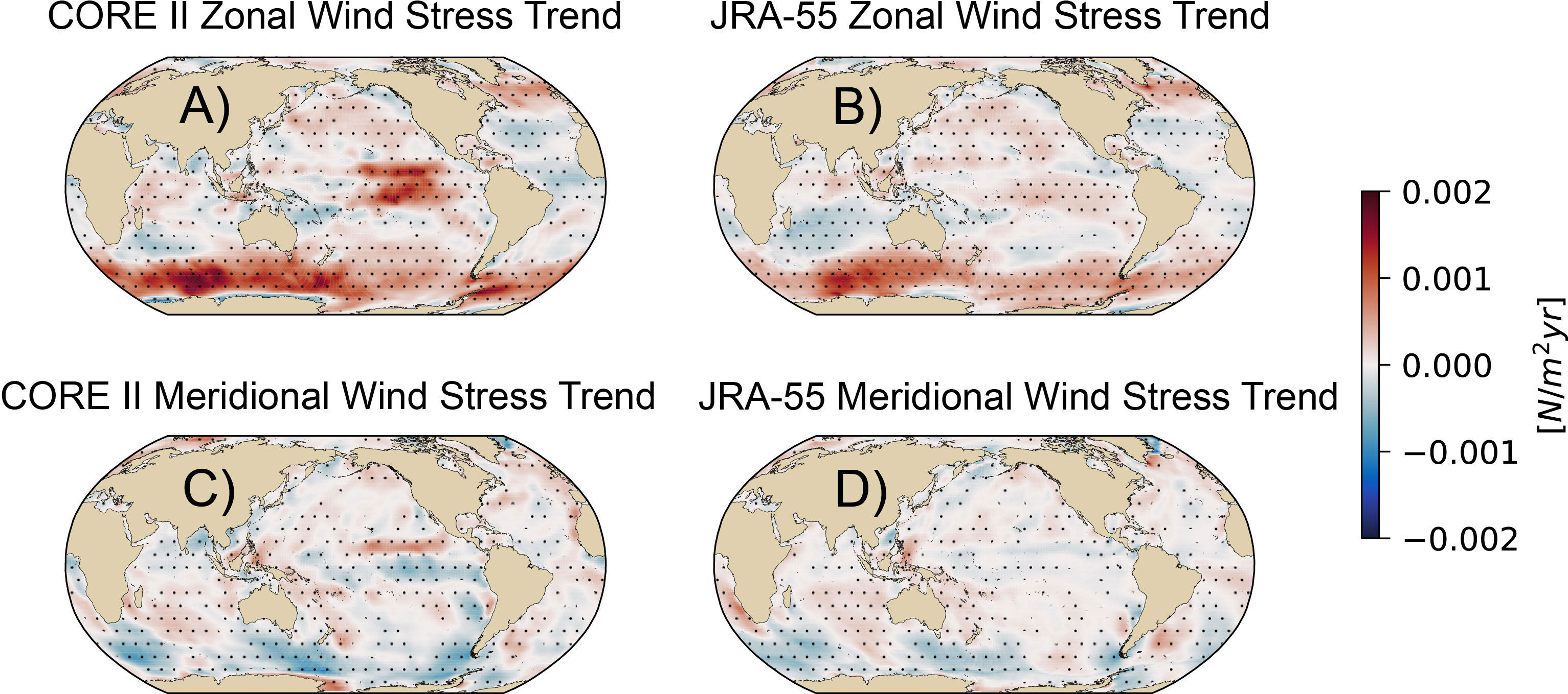
Figure 12 Linear trend of zonal and meridional wind stress fields from the CORE-II (A, C) and JRA-55 (B, D) atmospheric forcing used for the OMIP1 and OMIP2 simulations. Linear trend calculation period for each simulation is 1958-2007 for the CORE-II, and 1969-2018 for the JRA-55 wind stress fields respectively. The region with black dots show locations of trend statistically significant at the 95% confidence level based on a modified Mann-Kendall test.

4.2 Models’ equilibrium states and spin-up

Differences between OMIP and CMIP6 Historical simulations include the models’ equilibrium states. The CMIP6 Historical simulations are less likely to be impacted by model drift compared to the OMIP simulations due to the longer spin-up used in CMIP6 Historical simulations. In addition, the coupled CMIP6 Historical simulations could reach surface equilibrium faster compared to the OMIP simulations as any oceanic heat loss (gain) has an opposing effect on the atmospheric temperature whereas changes in sea surface temperature in the OMIP simulations do not feedback on the atmosphere. These spin-up procedures and feedback could have major impacts on regional changes.

The OMIP simulations are spun-up based on the recent historical forcing (i.e. atmospheric reanalysis for the past 50 years or so), which likely brings the background mean states to modern conditions. This is a major difference from the CMIP6 Historical simulations, which are based on the pre-industrial spun-up states of the ocean. This hypothesis has been tested in a recent study (Huguenin et al., 2022) for a specific modeling study of OHC, which showed that the background mean state of the ocean model is important for simulating historical ocean heat uptake. This approach should be tested with multi-model simulations. We hypothesize that a similar effect applies for simulating changes in the ocean O₂ content, as well as other biogeochemical tracers and processes (e.g. changes in the ocean carbon and nitrogen inventories).

4.3 Implications and future strategy

The CMIP6 Historical simulations show that the state-of-the art models have the potential to simulate historical deoxygenation in line with one of the most recent observational estimates. However, model spinup strategy and the dependency of the ocean circulation and biogeochemical responses on the atmospheric forcing could strongly bias the simulated O₂ changes. We thus propose for the next multi-modeling projects to coordinate forced ocean-only model simulations with a model spin-up strategy that employs a pre-industrial-like atmospheric forcing to achieve background mean states close to pre-industrial conditions. The potential experimental design could be based on an ocean model spin-up using the corrected atmospheric forcing used in the recent study by Huguenin et al., 2022. In this protocol, the corrected atmospheric forcing product uses air temperature and shortwave radiation adjusted to pre-industrial states from the recent IPCC report. This adjusted forcing successfully simulates global OHC during the historical era in the ACCESS-OM2 (one of the models analyzed in this study), which is currently weaker in the standard OMIP2 simulations (see Figure 3B and Huguenin et al., 2022). The similar approach should be tested using a suite of CMIP6 models, extending our simulations and analysis to other ocean biogeochemical tracers.

An alternative route may include using pre-industrial atmospheric forcing from the coupled simulations from each model participating in CMIP6 DECK simulations (Eyring et al., 2016). For either option, it is important to explore the ocean biogeochemical response to different background mean states using a suite of models to elucidate how ocean biogeochemistry responded in recent decades. Coordinated sensitivity experiments based on perturbed atmospheric forcing will enable us to further elucidate the mechanisms controlling the multi-decadal O₂ variability and trend (and factors leading to biases in the current simulations). Wind perturbation experiments, such as changing the magnitudes of zonal wind in the tropical Pacific Ocean, Southern Ocean, etc., built upon the previous sensitivity studies with specific models, for example from (Duteil et al., 2018) and (Ridder and England, 2014) will further elucidate how “common” atmospheric forcing biases leads to O₂ and ocean biogeochemistry biases in climatological mean states and long-term changes. Exploring O₂ variability driven by major climate modes, such as the Pacific Decadal Oscillation (PDO) and El Niño Southern Oscillation (ENSO) should also be explored on top of these sensitivity experiments (e.g. Deutsch et al., 2011; Ito and Deutsch, 2013; Deutsch et al., 2014; Eddebbar et al., 2017; Duteil et al., 2018; Ito et al., 2019; Poupon et al., 2023).

Ocean biogeochemistry models are known to have major issues in simulating the observed patterns and magnitude of global ocean deoxygenation in past decades (Stramma et al., 2012; Oschlies et al., 2017). Our analysis shows some improvements in simulating the observed global ocean deoxygenation. The observational datasets contains major uncertainties, with varying rates of O₂ loss across studies from the estimates of Ito et al. (2017) to more conservative estimates of Schmidtko et al. (2017) and Ito (2022). Recent efforts to combine existing datasets and new observations from autonomous floats e.g. Addey (2022) along with more robust quantification of uncertainties associated with data coverage and interpolation, alongside improved comparisons to models will be critical for a comprehensive assessment. Despite their shortcoming, forced ocean model simulations remain highly useful tools, particularly in understanding the drivers of internal climate variability in the O₂ content and distributions (e.g. Ito et al., 2019; Buchanan and Tagliabue, 2021). To maximize their use, future coordinated model experiments should highlight the choice of spin-up strategy for ocean biogeochemistry to achieve pre-industrial like ocean states for O₂ as well as other ocean biogeochemical cycles. The cyclic forcing (as in OMIP simulations) and associated discontinuity in solubility and ocean ventilation change could impact the ocean carbon cycle, and this could be explored quantitatively in future work. More detailed regional analysis is also needed to understand the mechanisms regulating global O₂ levels, particularly how ocean circulation and biological processes induce region-specific changes.

Data availability statement

Publicly available datasets were analyzed in this study. The CMIP6 and OMIP data can be found here: https://esgf-node.llnl.gov/search/cmip6/. The gridded observational dissolved oxygen dataset can be found in the websites (https://o2.eas.gatech.edu/data.html; https://www.bco-dmo.org/dataset/816978). Ocean temperature and salinity data could be found here: https://www.cen.uni-hamburg.de/en/icdc/data/ocean.html. Cheng’s dataset can be found here: http://www.ocean.iap.ac.cn/ and Ishii’s ocean heat content dataset can be found at the Japan Meteorological Agency’s (JMA) website: https://www.data.jma.go.jp/gmd/kaiyou/english/ohc/ohc_global_en.html.

Author contributions

YT led the study, and conducted the design of the study, data analysis, interpretation, and writing of the manuscript in collaboration with TI, JT, and YE. All authors supported on sharing and processing the model output and commented on the manuscript. All authors contributed to the article and approved the submitted version.

Funding

YT is supported as part of the Energy Exascale Earth System Model project, funded by the U.S. Department of Energy, Office of Science, Office of Biological and Environmental Research and a NERC-NSF grant (C-STREAMS, reference NE/W009579/1). This research was also supported by the Horizon 2020 research and innovation programme under grant agreement No. 641816 (CRESCENDO). This project (TI) has received funding from the European Union’s Horizon 2020 research and innovation programme under grant agreement No. 820989 (COMFORT), under grant agreement No. 101003536 (ESM2025–Earth System Models for the Future), and under grant agreement No. 821003 (4C). JT acknowledges Research Council of Norway funded project CE2COAST (318477) and OceanICU project under grant agreement no. 101083922. JT and JS were also supported by the Norwegian Research Council (project INES, grant no. 270061). YAE acknowledges funding support from the National Science Foundation OCE grant number 1948599. MB and TL received funding from the Italian Ministry MIUR through the JPI project CE2COAST, grant no. 318477. JP and AY were supported by the UK National Environmental Research Council funding under the ESM LTSM (NE/N018036/1), TerraFIRMA (NE/ W004895/1) and CLASS (NE/R015953/1) projects. MW and HTa were supported by MEXT program for the advanced studies of climate change projection (SENTAN) Grant Numbers JPMXD0722680395 and JPMXD0722681344.

Acknowledgments

The submission has been approved and assigned LA-UR number LA-UR-22-29410. This research used resources of the National Energy Research Scientific Computing Center, a DOE Office of Science User Facility supported by the Office of Science of the U.S. Department of Energy under Contract No. DE-AC02-05CH11231. We thank Charles Stock and Dave Munday for the comments on the manuscript and Taka Ito for the early discussion on observational dataset.

Conflict of interest

The authors declare that the research was conducted in the absence of any commercial or financial relationships that could be construed as a potential conflict of interest.

Publisher’s note

All claims expressed in this article are solely those of the authors and do not necessarily represent those of their affiliated organizations, or those of the publisher, the editors and the reviewers. Any product that may be evaluated in this article, or claim that may be made by its manufacturer, is not guaranteed or endorsed by the publisher.

Supplementary material

The Supplementary Material for this article can be found online at: https://www.frontiersin.org/articles/10.3389/fmars.2023.1139917/full#supplementary-material

References

Addey C. I. (2022). Using biogeochemical argo floats to understand ocean carbon and oxygen dynamics. Nat. Rev. Earth Environ. 3, 739. doi: 10.1038/s43017-022-00341-5

CrossRef Full Text | Google Scholar

Balmaseda M. A., Mogensen K., Weaver A. T. (2013). Evaluation of the ECMWF ocean reanalysis system ORAS4. Q. J. R. meteorological Soc. 139, 1132–1161. doi: 10.1002/qj.2063

CrossRef Full Text | Google Scholar

Berthet S., Jouanno J., Séférian R., Gehlen M., Llovel W. (2023). ). How does the phytoplankton–light feedback affect the marine n 2 o inventory? Earth System Dynamics 14, 399–412. doi: 10.5194/esd-14-399-2023

CrossRef Full Text | Google Scholar

Berthet S., Séférian R., Bricaud C., Chevallier M., Voldoire A., Ethé C. (2019). Evaluation of an online grid-coarsening algorithm in a global eddy-admitting ocean biogeochemical model. J. Adv. Modeling Earth Syst. 11, 1759–1783. doi: 10.1029/2019MS001644

CrossRef Full Text | Google Scholar

Bopp L., Le Quéré C., Heimann M., Manning A. C., Monfray P. (2002). Climate-induced oceanic oxygen fluxes: Implications for the contemporary carbon budget. Global Biogeochemical Cycles 16, 6–1–6–13. doi: 10.1029/2001GB001445

CrossRef Full Text | Google Scholar

Bopp L., Resplandy L., Orr J. C., Doney S. C., Dunne J. P., Gehlen M., et al. (2013). Multiple stressors of ocean ecosystems in the 21st century: projections with CMIP5 models. Biogeosciences 10, 6225–6245. doi: 10.5194/bg-10-6225-2013

CrossRef Full Text | Google Scholar

Bopp L., Resplandy L., Untersee A., Le Mezo P., Kageyama M. (2017). Ocean (de) oxygenation from the last glacial maximum to the twenty-first century: insights from earth system models. Philos. Trans. R. Soc. A: Mathematical Phys. Eng. Sci. 375, 20160323. doi: 10.1098/rsta.2016.0323

CrossRef Full Text | Google Scholar

Boucher O., Servonnat J., Albright A. L., Aumont O., Balkanski Y., Bastrikov V., et al. (2020). Presentation and evaluation of the IPSL-CM6A-LR climate model. J. Adv. Modeling Earth Syst. 12, e2019MS002010. doi: 10.1029/2019MS002010

CrossRef Full Text | Google Scholar

Breitburg D., Levin L. A., Oschlies A., Grégoire M., Chavez F. P., Conley D. J., et al. (2018). Declining oxygen in the global ocean and coastal waters. Science 359, eaam7240. doi: 10.1126/science.aam7240

PubMed Abstract | CrossRef Full Text | Google Scholar

Buchanan P. J., Tagliabue A. (2021). The regional importance of oxygen demand and supply for historical ocean oxygen trends. Geophysical Res. Lett. 48, e2021GL094797. doi: 10.1029/2021GL094797

CrossRef Full Text | Google Scholar

Buitenhuis E. T., Le Quere C., Bednaršek N., Schiebel R. (2019). Large contribution of pteropods to shallow CaCO₃ export. Global Biogeochemical Cycles 33, 458–468. doi: 10.1029/2018GB006110

CrossRef Full Text | Google Scholar

Burrows S., Maltrud M., Yang X., Zhu Q., Jeffery N., Shi X., et al. (2020). The DOE E3SM v1. 1 biogeochemistry configuration: Description and simulated ecosystem-climate responses to historical changes in forcing. J. Adv. Modeling Earth Syst. 12, e2019MS001766. doi: 10.1029/2019MS001766

CrossRef Full Text | Google Scholar

Busecke J. J., Resplandy L., Ditkovsky S. J., John J. G. (2022). Diverging fates of the pacific ocean oxygen minimum zone and its core in a warming world. AGU Adv. 3, e2021AV000470. doi: 10.1029/2021AV000470

CrossRef Full Text | Google Scholar

Busecke J. J., Resplandy L., Dunne J. P. (2019). The equatorial undercurrent and the oxygen minimum zone in the pacific. Geophysical Res. Lett. 46, 6716–6725. doi: 10.1029/2019GL082692

CrossRef Full Text | Google Scholar

Cabré A., Marinov I., Bernardello R., Bianchi D. (2015). Oxygen minimum zones in the tropical pacific across CMIP5 models: mean state differences and climate change trends. Biogeosciences 12, 5429–5454. doi: 10.5194/bg-12-5429-2015

CrossRef Full Text | Google Scholar

Canadell J. G., Monteiro P. M., Costa M. H., Da Cunha L. C., Cox P. M., Alexey V., et al. (2021). Global carbon and other biogeochemical cycles and feedbacks. In Climate Change 2021: The Physical Science Basis. Contribution of Working Group I to the Sixth Assessment Report of the Intergovernmental Panel on Climate Change Masson-Delmotte V., Zhai P., Pirani A., Connors S.L., Péan C., Berger S., et al (eds.)]. Cambridge, United Kingdom and New York, NY, USA: Cambridge University Press, pp. 673–816. doi: 10.1017/9781009157896.007a

CrossRef Full Text | Google Scholar

Cheng L., von Schuckmann K., Abraham J. P., Trenberth K. E., Mann M. E., Zanna L., et al. (2022). Past and future ocean warming. Nat. Rev. Earth Environ. 3, 776–794. doi: 10.1038/s43017-022-00345-1

CrossRef Full Text | Google Scholar

Cherchi A., Fogli P. G., Lovato T., Peano D., Iovino D., Gualdi S., et al. (2019). Global mean climate and main patterns of variability in the CMCC-CM2 coupled model. J. Adv. Modeling Earth Syst. 11, 185–209. doi: 10.1029/2018MS001369

CrossRef Full Text | Google Scholar

Christian J. R., Denman K. L., Hayashida H., Holdsworth A. M., Lee W. G., Riche O. G., et al. (2022). Ocean biogeochemistry in the canadian earth system model version 5.0.3: CanESM5 and CanESM5-CanOE. Geoscientific Model. Dev. 15, 4393–4424. doi: 10.5194/gmd-15-4393-2022

CrossRef Full Text | Google Scholar

Codispoti L. A. (1995). Is the ocean losing nitrate? Nature 376, 724–724. doi: 10.1038/376724a0

CrossRef Full Text | Google Scholar

Cooley S., Schoeman D., Bopp L., Boyd P., Donner S., Ghebrehiwet D., et al. (2022). “Ocean and coastal ecosystems and their services,” in Climate change 2022: impacts, adaptation, and vulnerability. Contribution of working group II to the sixth assessment report of the intergovernmental panel on climate change Pörtner H.-O., Roberts D.C., Tignor M., Poloczanska E.S., Mintenbeck K., Alegría A., et al (eds.)].Cambridge, UK and New York, NY, USA: Cambridge University Press, pp. 379–550. doi: 10.1017/9781009325844.005

CrossRef Full Text | Google Scholar

Danabasoglu G., Lamarque J.-F., Bacmeister J., Bailey D., DuVivier A., Edwards J., et al. (2020). The community earth system model version 2 (CESM2). J. Adv. Modeling Earth Syst. 12, e2019MS001916. doi: 10.1029/2019MS001916

CrossRef Full Text | Google Scholar

Danabasoglu G., Yeager S. G., Bailey D., Behrens E., Bentsen M., Bi D., et al. (2014). North atlantic simulations in coordinated ocean-ice reference experiments phase ii (core-ii). part i: mean states. Ocean Model. 73, 76–107. doi: 10.1016/j.ocemod.2013.10.005

CrossRef Full Text | Google Scholar

Deser C., Lehner F., Rodgers K. B., Ault T., Delworth T. L., DiNezio P. N., et al. (2020). Insights from earth system model initial-condition large ensembles and future prospects. Nat. Climate Change 10, 277–286. doi: 10.1038/s41558-020-0731-2

CrossRef Full Text | Google Scholar

Deutsch C., Berelson W., Thunell R., Weber T., Tems C., McManus J., et al. (2014). Centennial changes in north pacific anoxia linked to tropical trade winds. Science 345, 665–668. doi: 10.1126/science.1252332

PubMed Abstract | CrossRef Full Text | Google Scholar

Deutsch C., Brix H., Ito T., Frenzel H., Thompson L. (2011). Climate-forced variability of ocean hypoxia. science 333, 336–339. doi: 10.1126/science.1202422

PubMed Abstract | CrossRef Full Text | Google Scholar

Deutsch C., Ferrel A., Seibel B., Pörtner H.-O., Huey R. B. (2015). Climate change tightens a metabolic constraint on marine habitats. Science 348, 1132–1135. doi: 10.1126/science.aaa1605

PubMed Abstract | CrossRef Full Text | Google Scholar

Deutsch C., Penn J. L., Verberk W. C., Inomura K., Endress M.-G., Payne J. L. (2022). Impact of warming on aquatic body sizes explained by metabolic scaling from microbes to macrofauna. Proc. Natl. Acad. Sci. 119, e2201345119. doi: 10.1073/pnas.2201345119

CrossRef Full Text | Google Scholar

Döscher R., Acosta M., Alessandri A., Anthoni P., Arsouze T., Bergman T., et al. (2022). The EC-Earth3 earth system model for the coupled model intercomparison project 6. Geoscientific Model. Dev. 15, 2973–3020. doi: 10.5194/gmd-15-2973-2022

CrossRef Full Text | Google Scholar

Dunne J. P., Bociu I., Bronselaer B., Guo H., John J., Krasting J., et al. (2020b). Simple global ocean biogeochemistry with light, iron, nutrients and gas version 2 (BLINGv2): Model description and simulation characteristics in GFDL’s CM4.0. J. Adv. Modeling Earth Syst. 12, e2019MS002008. doi: 10.1029/2019MS002008

CrossRef Full Text | Google Scholar

Dunne J., Horowitz L., Adcroft A., Ginoux P., Held I., John J., et al. (2020a). The GFDL earth system model version 4.1 (GFDL-ESM 4.1): Overall coupled model description and simulation characteristics. J. Adv. Modeling Earth Syst. 12, e2019MS002015. doi: 10.1029/2019MS002015

CrossRef Full Text | Google Scholar

Duteil O., Oschlies A., Böning C. W. (2018). Pacific decadal oscillation and recent oxygen decline in the eastern tropical pacific ocean. Biogeosciences 15, 7111–7126. doi: 10.5194/bg-15-7111-2018

CrossRef Full Text | Google Scholar

Eddebbar Y. A., Long M. C., Resplandy L., Rödenbeck C., Rodgers K. B., Manizza M., et al. (2017). Impacts of ENSO on air-sea oxygen exchange: Observations and mechanisms. Global Biogeochemical Cycles 31, 901–921. doi: 10.1002/2017GB005630

CrossRef Full Text | Google Scholar

Eddebbar Y. A., Rodgers K. B., Long M. C., Subramanian A. C., Xie S.-P., Keeling R. F. (2019). El Niño–like physical and biogeochemical ocean response to tropical eruptions. J. Climate 32, 2627–2649. doi: 10.1175/JCLI-D-18-0458.1

CrossRef Full Text | Google Scholar

Eddebbar Y., Subramanian A., Whitt D., Long M., Verdy A., Mazloff M., et al. (2021). Seasonal modulation of dissolved oxygen in the equatorial pacific by tropical instability vortices. J. Geophysical Research: Oceans 126, e2021JC017567. doi: 10.1029/2021JC017567

CrossRef Full Text | Google Scholar

Emerson S. R., Hamme R. C. (2022). Chemical oceanography (Cambridge, United Kingdom: Cambridge University Press).

Google Scholar

Eyring V., Bony S., Meehl G. A., Senior C. A., Stevens B., Stouffer R. J., et al. (2016). Overview of the coupled model intercomparison project phase 6 (CMIP6) experimental design and organization. Geoscientific Model. Dev. 9, 1937–1958. doi: 10.5194/gmd-9-1937-2016

CrossRef Full Text | Google Scholar

Fay A. R., McKinley G. A., Lovenduski N. S., Eddebbar Y., Levy M. N., Long M. C., et al. (2023). Immediate and long-lasting impacts of the mt. pinatubo eruption on ocean oxygen and carbon inventories. Global Biogeochemical Cycles 37, e2022GB007513. doi: 10.1029/2022GB007513

CrossRef Full Text | Google Scholar

Friedlingstein P., Jones M. W., O’sullivan M., Andrew R. M., Hauck J., Peters G. P., et al. (2019). Global carbon budget 2019. Earth System Sci. Data 11, 1783–1838. doi: 10.5194/essd-11-1783-2019

CrossRef Full Text | Google Scholar

Garcia H. E., Gordon L. I. (1992). Oxygen solubility in seawater: Better fitting equations. Limnology oceanography 37, 1307–1312. doi: 10.4319/lo.1992.37.6.1307

CrossRef Full Text | Google Scholar

Garcia H., Weathers K., Paver C., Smolyar I., Boyer T., Locarnini M., et al. (2019). World ocean atlas 2018, volume 3: dissolved oxygen, apparent oxygen utilization, and dissolved oxygen saturation. Mishonov Technical Editor. NOAA Atlas NESDIS 83, 38 pp. doi: 10.7289/V5XG9P2W

CrossRef Full Text | Google Scholar

Gebbie G., Huybers P. (2012). The mean age of ocean waters inferred from radiocarbon observations: Sensitivity to surface sources and accounting for mixing histories. J. Phys. Oceanography 42, 291–305. doi: 10.1175/JPO-D-11-043.1

CrossRef Full Text | Google Scholar

Gouretski V., Reseghetti F. (2010). On depth and temperature biases in bathythermograph data: Development of a new correction scheme based on analysis of a global ocean database. Deep Sea Res. Part I: Oceanographic Res. Papers 57, 812–833. doi: 10.1016/j.dsr.2010.03.011

CrossRef Full Text | Google Scholar

Grégoire M., Garçon V., Garcia H., Breitburg D., Isensee K., Oschlies A., et al. (2021). A global ocean oxygen database and atlas for assessing and predicting deoxygenation and ocean health in the open and coastal ocean. Front. Mar. Sci. 8, 724913. doi: 10.3389/fmars.2021.724913

CrossRef Full Text | Google Scholar

Griffies S. M., Danabasoglu G., Durack P. J., Adcroft A. J., Balaji V., Böning C. W., et al. (2016). OMIP contribution to CMIP6: Experimental and diagnostic protocol for the physical component of the Ocean Model Intercomparison Project. Geoscientific Model. Dev. 9, 3231–3296. doi: 10.5194/gmd-9-3231-2016

CrossRef Full Text | Google Scholar

Gruber N. (2011). Warming up, turning sour, losing breath: ocean biogeochemistry under global change. Philos. Trans. R. Soc. A: Mathematical Phys. Eng. Sci. 369, 1980–1996. doi: 10.1098/rsta.2011.0003

CrossRef Full Text | Google Scholar

Hajima T., Watanabe M., Yamamoto A., Tatebe H., Noguchi M. A., Abe M., et al. (2020). Development of the MIROC-ES2L earth system model and the evaluation of biogeochemical processes and feedbacks. Geoscientific Model. Dev. 13, 2197–2244. doi: 10.5194/gmd-13-2197-2020

CrossRef Full Text | Google Scholar

Held I., Guo H., Adcroft A., Dunne J., Horowitz L., Krasting J., et al. (2019). Structure and performance of GFDL’s CM4.0 climate model. J. Adv. Modeling Earth Syst. 11, 3691–3727. doi: 10.1029/2019MS001829

CrossRef Full Text | Google Scholar

Helm K. P., Bindoff N. L., Church J. A. (2011). Observed decreases in oxygen content of the global ocean. Geophysical Res. Lett. 38, L23602. doi: 10.1029/2011GL049513

CrossRef Full Text | Google Scholar

Huguenin M. F., Holmes R. M., England M. H. (2022). Drivers and distribution of global ocean heat uptake over the last half century. Nat. Commun. 13, 1–11. doi: 10.1038/s41467-022-32540-5

PubMed Abstract | CrossRef Full Text | Google Scholar

Hussain M., Mahmud I. (2019). pymannkendall: a python package for non parametric mann kendall family of trend tests. J. Open Source Software 4, 1556. doi: 10.21105/joss.01556

CrossRef Full Text | Google Scholar

Ilyina T., Six K. D., Segschneider J., Maier-Reimer E., Li H., Núñez-Riboni I. (2013). Global ocean biogeochemistry model HAMOCC: Model architecture and performance as component of the MPI-Earth system model in different CMIP5 experimental realizations. J. Adv. Modeling Earth Syst. 5, 287–315. doi: 10.1029/2012MS000178

CrossRef Full Text | Google Scholar

IPCC. (2019). “The ocean and cryosphere in a changing climate,” in IPCC special report on the ocean and cryosphere in a changing climate Pörtner H.-O., Roberts D. C., Masson-Delmotte V., Zhai P., Tignor M., Poloczanska E., et al (eds.)]. Cambridge, UK and New York, NY, USA: Cambridge University Press, 755 pp. doi: 10.1017/9781009157964

CrossRef Full Text | Google Scholar

Ishii M., Fukuda Y., Hirahara S., Yasui S., Suzuki T., Sato K. (2017). Accuracy of global upper ocean heat content estimation expected from present observational data sets. Sola 13, 163–167. doi: 10.2151/sola.2017-030

CrossRef Full Text | Google Scholar

Ito T. (2022). Optimal interpolation of global dissolved oxygen: 1965–2015. Geosci. Data J. 9, 167–176. doi: 10.1002/gdj3.130

CrossRef Full Text | Google Scholar

Ito T., Deutsch C. (2013). Variability of the oxygen minimum zone in the tropical north pacific during the late twentieth century. Global Biogeochemical Cycles 27, 1119–1128. doi: 10.1002/2013GB004567

CrossRef Full Text | Google Scholar

Ito T., Garcia H. E., Wang Z., Minobe S., Long M. C., Cebrian J., et al. (2023). Underestimation of global o 2 loss in optimally interpolated historical ocean observations. Biogeosciences Discussions 2023, 1–22. doi: 10.5194/bg-2023-72

CrossRef Full Text | Google Scholar

Ito T., Long M. C., Deutsch C., Minobe S., Sun D. (2019). Mechanisms of low-frequency oxygen variability in the north pacific. Global Biogeochemical Cycles 33, 110–124. doi: 10.1029/2018GB005987

CrossRef Full Text | Google Scholar

Ito T., Minobe S., Long M. C., Deutsch C. (2017). Upper ocean O₂ trends: 1958–2015. Geophysical Res. Lett. 44, 4214–4223. doi: 10.1002/2017GL073613

CrossRef Full Text | Google Scholar

Kalnay E., Kanamitsu M., Kistler R., Collins W., Deaven D., Gandin L., et al. (1996). The NCEP/NCAR 40-year reanalysis project. Bull. Am. meteorological Soc. 77, 437–472. doi: 10.1175/1520-0477(1996)077<0437:TNYRP>2.0.CO;2

CrossRef Full Text | Google Scholar

Keeling R. F., Garcia H. E. (2002). The change in oceanic O₂ inventory associated with recent global warming. Proc. Natl. Acad. Sci. 99, 7848–7853. doi: 10.1073/pnas.122154899

CrossRef Full Text | Google Scholar

Keeling R. F., Körtzinger A., Gruber N. (2010). Ocean deoxygenation in a warming world. Annu. Rev. Mar. Sci. 2, 199–229. doi: 10.1146/annurev.marine.010908.163855

CrossRef Full Text | Google Scholar

Keil P., Mauritsen T., Jungclaus J., Hedemann C., Olonscheck D., Ghosh R. (2020). Multiple drivers of the north atlantic warming hole. Nat. Climate Change 10, 667–671. doi: 10.1038/s41558-020-0819-8

CrossRef Full Text | Google Scholar

Khatiwala S., Primeau F., Holzer M. (2012). Ventilation of the deep ocean constrained with tracer observations and implications for radiocarbon estimates of ideal mean age. Earth Planetary Sci. Lett. 325, 116–125. doi: 10.1016/j.epsl.2012.01.038

CrossRef Full Text | Google Scholar

Kiss A. E., Hogg A. M., Hannah N., Boeira Dias F., Brassington G. B., Chamberlain M. A., et al. (2020). ACCESS-OM2 v1.0: a global ocean–sea ice model at three resolutions. Geoscientific Model. Dev. 13, 401–442. doi: 10.5194/gmd-13-401-2020

CrossRef Full Text | Google Scholar

Kwiatkowski L., Torres O., Bopp L., Aumont O., Chamberlain M., Christian J. R., et al. (2020). Twenty-first century ocean warming, acidification, deoxygenation, and upper-ocean nutrient and primary production decline from CMIP6 model projections. Biogeosciences 17, 3439–3470. doi: 10.5194/bg-17-3439-2020

CrossRef Full Text | Google Scholar

Laffoley D., Baxter J. M. (2019). Ocean deoxygenation: Everyone’s problem-causes, impacts, consequences and solutions (Switzerland: IUCN Gland).

Google Scholar

Large W., Yeager S. (2009). The global climatology of an interannually varying air-sea flux data set. Climate dynamics 33, 341–364. doi: 10.1007/s00382-008-0441-3

CrossRef Full Text | Google Scholar

Le Quéré C., Buitenhuis E. T., Moriarty R., Alvain S., Aumont O., Bopp L., et al. (2016). Role of zooplankton dynamics for southern ocean phytoplankton biomass and global biogeochemical cycles. Biogeosciences 13, 4111–4133. doi: 10.5194/bg-13-4111-2016

CrossRef Full Text | Google Scholar

Levin L. A. (2018). Manifestation, drivers, and emergence of open ocean deoxygenation. Annu. Rev. Mar. Sci. 10, 229–260. doi: 10.1146/annurev-marine-121916-063359

CrossRef Full Text | Google Scholar

Levitus S., Antonov J. I., Boyer T. P., Baranova O. K., Garcia H. E., Locarnini R. A., et al. (2012). World ocean heat content and thermosteric sea level change (0–2000 m), 1955–2010. Geophysical Res. Lett. 39, L10603. doi: 10.1029/2012GL051106

CrossRef Full Text | Google Scholar

Long M. C., Deutsch C., Ito T. (2016). Finding forced trends in oceanic oxygen. Global Biogeochemical Cycles 30, 381–397. doi: 10.1002/2015GB005310

CrossRef Full Text | Google Scholar

Long M. C., Moore J. K., Lindsay K., Levy M., Doney S. C., Luo J. Y., et al. (2021). Simulations with the marine biogeochemistry library (MARBL). J. Adv. Modeling Earth Syst. 13, e2021MS002647. doi: 10.1029/2021MS002647

CrossRef Full Text | Google Scholar

Longhurst A. R., Harrison W. G. (1989). The biological pump: profiles of plankton production and consumption in the upper ocean. Prog. Oceanography 22, 47–123. doi: 10.1016/0079-6611(89)90010-4

CrossRef Full Text | Google Scholar

Lovato T., Peano D., Butenschön M., Materia S., Iovino D., Scoccimarro E., et al. (2022). CMIP6 simulations with the cmcc earth system model (CMCC-ESM2). J. Adv. Modeling Earth Syst. 14, e2021MS002814. doi: 10.1029/2021MS002814

CrossRef Full Text | Google Scholar

Martínez-Moreno J., Hogg A. M., England M. H., Constantinou N. C., Kiss A. E., Morrison A. K. (2021). Global changes in oceanic mesoscale currents over the satellite altimetry record. Nat. Climate Change 11, 397–403. doi: 10.1038/s41558-021-01006-9

CrossRef Full Text | Google Scholar

Mauritsen T., Bader J., Becker T., Behrens J., Bittner M., Brokopf R., et al. (2019). Developments in the MPI-M earth system model version 1.2 (MPI-ESM1.2) and its response to increasing co2. J. Adv. Modeling Earth Syst. 11, 998–1038. doi: 10.1029/2018MS001400

CrossRef Full Text | Google Scholar

Moore J. K., Doney S. C., Lindsay K. (2004). Upper ocean ecosystem dynamics and iron cycling in a global three-dimensional model. Global Biogeochemical Cycles 18, GB4028. doi: 10.1029/2004GB002220

CrossRef Full Text | Google Scholar

Mora C., Wei C.-L., Rollo A., Amaro T., Baco A. R., Billett D., et al. (2013). Biotic and human vulnerability to projected changes in ocean biogeochemistry over the 21st century. PloS Biol. 11, e1001682. doi: 10.1371/journal.pbio.1001682

PubMed Abstract | CrossRef Full Text | Google Scholar

Morée A. L., Clarke T. M., Cheung W. W., Frölicher T. L. (2023). Impact of deoxygenation and warming on global marine species in the 21st century. Biogeosciences 20, 2425–2454. doi: 10.5194/bg-20-2425-2023

CrossRef Full Text | Google Scholar

Morel F. M., Price N. (2003). The biogeochemical cycles of trace metals in the oceans. Science 300, 944–947. doi: 10.1126/science.1083545

PubMed Abstract | CrossRef Full Text | Google Scholar

Olsen A., Key R. M., Van Heuven S., Lauvset S. K., Velo A., Lin X., et al. (2016). The Global Ocean Data Analysis Project version 2 (GLODAPv2)–an internally consistent data product for the world ocean. Earth System Sci. Data 8, 297–323. doi: 10.5194/essd-8-297-2016

CrossRef Full Text | Google Scholar

Orr J. C., Najjar R. G., Aumont O., Bopp L., Bullister J. L., Danabasoglu G., et al. (2017). Biogeochemical protocols and diagnostics for the CMIP6 ocean model intercomparison project (OMIP). Geoscientific Model. Dev. 10, 2169–2199. doi: 10.5194/gmd-10-2169-2017

CrossRef Full Text | Google Scholar

Oschlies A., Brandt P., Stramma L., Schmidtko S. (2018). Drivers and mechanisms of ocean deoxygenation. Nat. Geosci. 11, 467–473. doi: 10.1038/s41561-018-0152-2

CrossRef Full Text | Google Scholar

Oschlies A., Duteil O., Getzlaff J., Koeve W., Landolfi A., Schmidtko S. (2017). Patterns of deoxygenation: sensitivity to natural and anthropogenic drivers. Philos. Trans. R. Soc. A: Mathematical Phys. Eng. Sci. 375, 20160325. doi: 10.1098/rsta.2016.0325

CrossRef Full Text | Google Scholar

Paulsen H., Ilyina T., Six K. D., Stemmler I. (2017). Incorporating a prognostic representation of marine nitrogen fixers into the global ocean biogeochemical model HAMOCC. J. Adv. Modeling Earth Syst. 9, 438–464. doi: 10.1002/2016MS000737

CrossRef Full Text | Google Scholar

Poli P., Hersbach H., Dee D. P., Berrisford P., Simmons A. J., Vitart F., et al. (2016). ERA-20C: An atmospheric reanalysis of the twentieth century. J. Climate 29, 4083–4097. doi: 10.1175/JCLI-D-15-0556.1

CrossRef Full Text | Google Scholar

Poupon M. A., Resplandy L., Lévy M., Bopp L. (2023). Pacific decadal oscillation influences tropical oxygen minimum zone extent and obscures anthropogenic changes. Geophysical Res. Lett. 50, e2022GL102123. doi: 10.1029/2022GL102123

CrossRef Full Text | Google Scholar

Rahmstorf S., Box J. E., Feulner G., Mann M. E., Robinson A., Rutherford S., et al. (2015). Exceptional twentieth-century slowdown in atlantic ocean overturning circulation. Nat. Climate Change 5, 475–480. doi: 10.1038/nclimate2554

CrossRef Full Text | Google Scholar

Rhein M., Steinfeldt R., Kieke D., Stendardo I., Yashayaev I. (2017). Ventilation variability of Labrador sea water and its impact on oxygen and anthropogenic carbon: a review. Philos. Trans. R. Soc. A: Mathematical Phys. Eng. Sci. 375, 20160321. doi: 10.1098/rsta.2016.0321

CrossRef Full Text | Google Scholar

Ridder N. N., England M. H. (2014). Sensitivity of ocean oxygenation to variations in tropical zonal wind stress magnitude. Global Biogeochemical Cycles 28, 909–926. doi: 10.1002/2013GB004708

CrossRef Full Text | Google Scholar

Schmidtko S., Stramma L., Visbeck M. (2017). Decline in global oceanic oxygen content during the past five decades. Nature 542, 335–339. doi: 10.1038/nature21399

PubMed Abstract | CrossRef Full Text | Google Scholar

Schulzweida U. (2022). Cdo user guide (2.3.0) Zenodo. doi: 10.5281/zenodo.7112925

CrossRef Full Text | Google Scholar

Séférian R., Berthet S., Yool A., Palmieri J., Bopp L., Tagliabue A., et al. (2020). Tracking improvement in simulated marine biogeochemistry between CMIP5 and CMIP6. Curr. Climate Change Rep. 6, 95–119. doi: 10.1007/s40641-020-00160-0

CrossRef Full Text | Google Scholar

Séférian R., Gehlen M., Bopp L., Resplandy L., Orr J. C., Marti O., et al. (2016). Inconsistent strategies to spin up models in CMIP5: implications for ocean biogeochemical model performance assessment. Geoscientific Model. Dev. 9, 1827–1851. doi: 10.5194/gmd-9-1827-2016

CrossRef Full Text | Google Scholar

Séférian R., Nabat P., Michou M., Saint-Martin D., Voldoire A., Colin J., et al. (2019). Evaluation of CNRM earth system model, CNRM-ESM2-1: Role of earth system processes in present-day and future climate. J. Adv. Modeling Earth Syst. 11, 4182–4227. doi: 10.1029/2019MS001791

CrossRef Full Text | Google Scholar

Sellar A. A., Jones C. G., Mulcahy J. P., Tang Y., Yool A., Wiltshire A., et al. (2019). UKESM1: Description and evaluation of the UK earth system model. J. Adv. Modeling Earth Syst. 11, 4513–4558. doi: 10.1029/2019MS001739

CrossRef Full Text | Google Scholar

Stock C. A., Dunne J. P., Fan S., Ginoux P., John J., Krasting J. P., et al. (2020). Ocean biogeochemistry in GFDL’s Earth System Model 4.1 and its response to increasing atmospheric CO₂. J. Adv. Modeling Earth Syst. 12, e2019MS002043. doi: 10.1029/2019MS002043

CrossRef Full Text | Google Scholar

Stramma L., Oschlies A., Schmidtko S. (2012). Mismatch between observed and modeled trends in dissolved upper-ocean oxygen over the last 50 yr. Biogeosciences 9, 4045–4057. doi: 10.5194/bg-9-4045-2012

CrossRef Full Text | Google Scholar

Swart N. C., Cole J. N., Kharin V. V., Lazare M., Scinocca J. F., Gillett N. P., et al. (2019). The canadian earth system model version 5 (CanESM5. 0.3). Geoscientific Model. Dev. 12, 4823–4873. doi: 10.5194/gmd-12-4823-2019

CrossRef Full Text | Google Scholar

Taboada F. G., Stock C. A., Griffies S. M., Dunne J., John J. G., Small R. J., et al. (2019). Surface winds from atmospheric reanalysis lead to contrasting oceanic forcing and coastal upwelling patterns. Ocean Model. 133, 79–111. doi: 10.1016/j.ocemod.2018.11.003

CrossRef Full Text | Google Scholar

Takano Y., Ito T., Deutsch C. (2018). Projected centennial oxygen trends and their attribution to distinct ocean climate forcings. Global Biogeochemical Cycles 32, 1329–1349. doi: 10.1029/2018GB005939

CrossRef Full Text | Google Scholar

Tjiputra J., Goris N., Lauvset S., Heinze C., Olsen A., Schwinger J., et al. (2018). Mechanisms and early detections of multidecadal oxygen changes in the interior subpolar north atlantic. Geophysical Res. Lett. 45, 4218–4229. doi: 10.1029/2018GL077096

CrossRef Full Text | Google Scholar

Tjiputra J. F., Negrel J., Olsen A. (2023). Early detection of anthropogenic climate change signals in the ocean interior. Sci. Rep. 13, 3006. doi: 10.1038/s41598-023-30159-0

PubMed Abstract | CrossRef Full Text | Google Scholar

Tjiputra J. F., Schwinger J., Bentsen M., Morée A. L., Gao S., Bethke I., et al. (2020). Ocean biogeochemistry in the Norwegian Earth System Model version 2 (NorESM2). Geoscientific Model. Dev. 13, 2393–2431. doi: 10.5194/gmd-13-2393-2020

CrossRef Full Text | Google Scholar

Tseng Y.-h., Lin H., Chen H.-c., Thompson K., Bentsen M., Böning C. W., et al. (2016). North and equatorial pacific ocean circulation in the core-ii hindcast simulations. Ocean Model. 104, 143–170. doi: 10.1016/j.ocemod.2016.06.003

CrossRef Full Text | Google Scholar

Tsujino H., Urakawa L. S., Griffies S. M., Danabasoglu G., Adcroft A. J., Amaral A. E., et al. (2020). Evaluation of global ocean-sea-ice model simulations based on the experimental protocols of the Ocean Model Intercomparison Project phase 2 (OMIP-2). Geoscientific Model. Dev. 13, 3643–3708. doi: 10.5194/gmd-13-3643-2020

CrossRef Full Text | Google Scholar

Tsujino H., Urakawa S., Nakano H., Small R. J., Kim W. M., Yeager S. G., et al. (2018). JRA-55 based surface dataset for driving ocean–sea-ice models (JRA55-do). Ocean Model. 130, 79–139. doi: 10.1016/j.ocemod.2018.07.002

CrossRef Full Text | Google Scholar

Urakawa L. S., Tsujino H., Nakano H., Sakamoto K., Yamanaka G., Toyoda T. (2020). The sensitivity of a depth-coordinate model to diapycnal mixing induced by practical implementations of the isopycnal tracer diffusion scheme. Ocean Model. 154, 101693. doi: 10.1016/j.ocemod.2020.101693

CrossRef Full Text | Google Scholar

Vaquer-Sunyer R., Duarte C. M. (2008). Thresholds of hypoxia for marine biodiversity. Proc. Natl. Acad. Sci. 105, 15452–15457. doi: 10.1073/pnas.0803833105

CrossRef Full Text | Google Scholar

Wright R. M., Le Quéré C., Buitenhuis E., Pitois S., Gibbons M. J. (2021). Role of jellyfish in the plankton ecosystem revealed using a global ocean biogeochemical model. Biogeosciences 18, 1291–1320. doi: 10.5194/bg-18-1291-2021

CrossRef Full Text | Google Scholar

Wunsch C., Heimbach P. (2008). How long to oceanic tracer and proxy equilibrium? Quaternary Sci. Rev. 27, 637–651. doi: 10.1016/j.quascirev.2008.01.006

CrossRef Full Text | Google Scholar

Yeager S., Danabasoglu G., Rosenbloom N., Strand W., Bates S., Meehl G., et al. (2018). Predicting near-term changes in the earth system: A large ensemble of initialized decadal prediction simulations using the community earth system model. Bull. Am. Meteorological Soc. 99, 1867–1886. doi: 10.1175/BAMS-D-17-0098.1

CrossRef Full Text | Google Scholar

Yool A., Palmiéri J., Jones C. G., de Mora L., Kuhlbrodt T., Popova E. E., et al. (2021). Evaluating the physical and biogeochemical state of the global ocean component of UKESM1 in CMIP6 historical simulations. Geoscientific Model. Dev. 14, 3437–3472. doi: 10.5194/gmd-14-3437-2021

CrossRef Full Text | Google Scholar

Yool A., Palmiéri J., Jones C., Sellar A., de Mora L., Kuhlbrodt T., et al. (2020). Spin-up of UK earth system model 1 (UKESM1) for CMIP6. J. Adv. Modeling Earth Syst. 12, e2019MS001933. doi: 10.1029/2019MS001933

CrossRef Full Text | Google Scholar

Yue S., Wang C. (2004). The Mann-Kendall test modified by effective sample size to detect trend in serially correlated hydrological series. Water Resour. Manage. 18, 201–218. doi: 10.1023/B:WARM.0000043140.61082.60

CrossRef Full Text | Google Scholar

Yukimoto S., Kawai H., Koshiro T., Oshima N., Yoshida K., Urakawa S., et al. (2019). The Meteorological Research Institute Earth System Model version 2.0, MRI-ESM2.0: Description and basic evaluation of the physical component. J. Meteorol. Soc. Jpn. 97, 931–965. doi: 10.2151/jmsj.2019-051

CrossRef Full Text | Google Scholar

Ziehn T., Chamberlain M. A., Law R. M., Lenton A., Bodman R. W., Dix M., et al. (2020). The Australian earth system model: ACCESS-ESM1.5. J. South. Hemisphere Earth Syst. Sci. 70, 193–214. doi: 10.1071/ES19035

CrossRef Full Text | Google Scholar