Estimation of the Manning’s n coefficient in multi-constituent tidal models by assimilating satellite observations with the adjoint data assimilation

1 Introduction

Tide is a ubiquitous oceanographic phenomenon in the global ocean (Wei et al., 2022) and is a significant source of power to drive the ocean interior mixing (Munk and Wunsch, 1998). Different from the tide in deep seas, the tide in shallow waters is pronouncedly effected by the bottom friction in the bottom boundary layer (Nicolle and Karpytchev, 2007), which is responsible for the dissipation of over 70% of the global tidal energy (Munk and Wunsch, 1998). The tide in shallow waters is an important research field of physical oceanography and is essential for ocean transport (Wei et al., 2022), coastal ocean engineering (Lee and Jeng, 2002; Chen et al., 2007), sediment and nutrient transport (Sana and Tanaka, 1997; Fan et al., 2019). Coastal tidal models have been the effective tool to simulate and predict the tide and to investigate the bottom friction dissipation in shallow waters. The bottom frictional stress in the coastal tidal models can be defined using a linear or quadratic drag law (Mayo et al., 2014). In the widely used quadratic drag law, the bottom frictional stress is a quadratic function of the bottom friction coefficient (BFC) and velocity (Taylor, 1920). BFC can be determined using the Manning’s n formulation and equal to gn²/h^1/3, where g is the acceleration due to gravity, h is the water depth, and n is the Manning’s n coefficient (Mayo et al., 2014). The Manning’s n coefficient is defined as multiple types of resistance to water flow because of bottom surface characteristics and is vital for accurate simulation and prediction of the tide in shallow coastal waters, whereas it cannot be directly measured and contains large amounts of uncertainties caused by the empirical estimation (Budgell, 1987; Mayo et al., 2014).

As an empirically derived model parameter, the Manning’s n coefficient in the tidal models can be estimated by the traditional trial and error method, but it is unfeasible especially for the spatially varying or spatially-temporally varying Manning’s n coefficients (Siripatana et al., 2018). Blakely et al. (2022) estimated the optimal constant Manning’s n coefficient and internal tide dissipation coefficient in every region in a global tide model using the sequential frictional parameter optimization process. With development of computer power and satellite remote sensing observational technology, estimation of Manning’s n coefficient using data assimilation becomes more realistic and feasible. Ding and Wang (2005) estimated the Manning’s n coefficient in the one-dimensional flow model of a river by assimilating the synthetic observations of discharges and stages with the optimal control theories and adjoint analysis. Hostache et al. (2010) identified the optimal Manning’s n coefficient in the Mosel River by assimilating the water level obtained from Synthetic Aperture Radar images of river inundation into a shallow-water flood model with the variational data assimilation method. Pedinotti et al. (2014) estimated the Manning’s n coefficient by assimilating virtual water level observations obtained from satellite data into a coupled land-surface hydrology model with the extended Kalman filter method. Sraj et al. (2014) estimated the Manning’s n coefficient in two-dimensional (2D) shallow water equations by assimilating buoy-observed water surface elevation with a Bayesian inverse modeling method. Mayo et al. (2014) estimated the spatially varying Manning’s n coefficient by assimilating the synthetic water elevation observations with a statistical data assimilation method. Demissie and Bacopoulos (2017) estimated the anisotropic Manning’s n coefficient by assimilating temporally and spatially varying velocity observations with nudging analysis. Graham et al. (2017) estimated the Manning’s n coefficient in a storm surge model by assimilating the maximum free surface elevations at observation stations with the measure-theoretic algorithm. Slivinski et al. (2017) estimated the Manning’s n coefficient in a multiple-inlet system by assimilating the observations of Lagrangian drifter trajectories with the ensemble Kalman filter. Siripatana et al. (2017) estimated the Manning’s n coefficient by assimilating synthetic observations in a simplified ebb shoal associated with an idealize inlet using the ensemble Kalman filter method and Markov chain Monte Carlo method. Siripatana et al. (2018) further quantified the spatially varying Manning’s n coefficients by assimilating synthetic observations of water elevation with a sequential data assimilation framework. Ziliani et al. (2019) estimated the two-dimensional Manning’s n coefficients in a flood model by assimilating real measurements of water depth with the ensemble Kalman filter. Warder et al. (2022) estimated the Manning’s n coefficient in the numerical model of Bristol Channel tidal dynamics by assimilating tidal harmonic data at 15 locations with a Bayesian inference algorithm.

The adjoint data assimilation is one of the classical data assimilation methods and has been widely used in the parameter estimation in oceanography (Navon, 1998; Fringer et al., 2019). Ullman and Wilson (1998) used the adjoint data assimilation to estimate the BFC directly by assimilating the Acoustic Doppler current profiler data. Heemink et al. (2002) applied the adjoint data assimilation to estimate the open boundary conditions, the spatially varying BFC and viscosity parameter, and the water depth in a three-dimensional shallow sea model by assimilating tidal gauge data and satellite altimeter data. Gao et al. (2015) used the adjoint data assimilation to simultaneously estimate the spatially varying BFC and internal tide dissipation coefficient in the South China Sea by assimilating the tidal harmonic constants derived from both tidal gauge stations and satellite altimeter crossover points. Wang et al. (2021a) estimated the temporally varying BFC in the Bohai Sea by assimilating satellite-retrieved tidal harmonic constants with the adjoint data assimilation. Wang et al. (2021b) estimated the spatially-temporally varying BFC in multi-constituent tidal model in the Bohai, Yellow and East China Seas (BYECS) by assimilating satellite altimeter data with the adjoint data assimilation. Compared to the depth independent BFC, the extra depth dependency in the Manning’s n formulation redistributes resistance to the inner shelf from the outer and mid shelf, leading to much better simulated results of tides in marginal seas when the global ocean tides are simulated (Blakely et al., 2022). It is necessary to estimate the Manning’s n coefficient in the marginal seas. However, the adjoint data assimilation has not been used to estimate the Manning’s n coefficient in the Chinese shallow coastal waters.

The tidal dynamics in the BYECS are complex and has been simulated by many researchers. However, the Manning’s n coefficient in the BYECS is traditionally set as constant or spatially varying based on personal experiences and has not been systematically estimated using the data assimilation method. Therefore, the applicability of estimating the Manning’s n coefficient in the BYECS with the adjoint data assimilation are not clear at present. In order to investigate the feasibility and effectiveness of adjoint data assimilation in estimating Manning’s n coefficient in the BYECS, twin experiments of assimilating synthetic satellite observations and practical experiments of assimilating real satellite observations are conducted in this study. Remaining sections of this paper is organized as follows: Section 2 introduces models, observations and procedure of estimating the Manning’s n coefficient; Section 3 describes the twin experiments to investigate the feasibility and effectiveness of estimating the Manning’s n coefficient; Section 4 illustrates the practical experiments to synchronously simulate the four principal tidal constituents in the BYECS by estimating the Manning’s n coefficient; Section 5 gives discussions; Section 6 summarizes the key finds with conclusion.

2 Models and observations

2.1 2D multi-constituent tidal model

The governing equations of the 2D multi-constituent tidal model are as follows (Wang et al., 2021b):

$\begin{array}{ll}\frac{\partial \zeta }{\partial t}+\frac{1}{a}\frac{\partial [(h+\zeta )u]}{\partial \lambda }+\frac{1}{a}\frac{\partial [(h+\zeta )v\cos \varphi ]}{\partial \varphi }=0& (1)\end{array}$

$\begin{array}{ll}\frac{\partial u}{\partial t}+\frac{u}{a}\frac{\partial u}{\partial \lambda }+\frac{v}{R}\frac{\partial u}{\partial \varphi }-\frac{uv\tan \varphi }{R}-fv+\frac{ku\sqrt{u^2+v^2}}{h+\zeta }-A\Delta u+\frac{g}{a}\frac{\partial (\zeta -\overline{\zeta })}{\partial \lambda }=0& (2)\end{array}$

$\begin{array}{ll}\frac{\partial v}{\partial t}+\frac{u}{a}\frac{\partial v}{\partial \lambda }+\frac{v}{R}\frac{\partial v}{\partial \varphi }+\frac{u^2\tan \varphi }{R}+fu+\frac{kv\sqrt{u^2+v^2}}{h+\zeta }-A\Delta v+\frac{g}{R}\frac{\partial (\zeta -\overline{\zeta })}{\partial \varphi }=0& (3)\end{array}$

where ζ is the sea surface elevation above the undisturbed sea level; t is time; λ and $\varphi$ are longitude and latitude, respectively; R is the radius of the earth; $a=R\cos \varphi$; h is the undisturbed water depth; u and v are the velocity components in the east and north, respectively; f is the Coriolis parameter; g is the acceleration due to gravity; k is the BFC; A is the horizontal eddy viscosity coefficient; Δ is the Laplace operator; $\Delta (u,v)=a^{-1}[a^{-1}{\partial }_{\lambda }({\partial }_{\lambda }(u,v))+R^{-1}{\partial }_{\varphi }(\cos \varphi {\partial }_{\varphi }(u,v))]$; and $\overline{\zeta }$ is the adjusted height of equilibrium tide.

The BFC k is calculated using the Manning’s n formulation, as follows:

$\begin{array}{ll}k=\frac{g}{C^2}=\frac{g}{{(\raisebox{1ex}{$h^{1/6}$}\!\left/ \!\raisebox{-1ex}{$n$}\right.)}^2}=\frac{g{n}^2}{h^{1/3}}& (4)\end{array}$

where C is the Chezy friction coefficient and n is the Manning’s n coefficient.

The initial condition is that both the sea surface elevation ζ and the velocity (u and v) are zero in the computational domain. At the closed land boundaries, the normal velocity is zero. At the open sea boundaries, the sea surface elevation ζ is caused by the principal tidal constituents and calculated as follows:

$\begin{array}{ll}\zeta (t)={\displaystyle \sum _{m=1}^M{F}_m{A}_m\cos ({\omega }_{m}t+V_m+U_m-G_m)}& (5)\end{array}$

where A and G are the amplitude and phase lag (UTC, the same below), respectively; F is the nodal factor; V is the initial phase angle of the equilibrium tide; U is the nodal angle; ω is the angular speed of the tidal constituent; m is the mth tidal constituent; and M is the number of the principal tidal constituents and can be specified according to the requirement. The specific number of the principal tidal constituents used in this study will be given when the model settings are described below. The harmonic constants (amplitude and phase lag) of the principal tidal constituents at the open sea boundaries are obtained from Oregon State University Tidal Inversion Software (Egbert and Erofeeva, 2002). The numerical schemes used for solving this 2D multi-constituent tidal model are the same as those in Lu and Zhang (2006).

2.2 Adjoint model

To evaluate the simulated errors, a cost function is defined based on the adjoint method and calculated as follows (Lu and Zhang, 2006; Zhang and Wang, 2014):

$\begin{array}{ll}J=\frac{1}{2}{K}_{\zeta }{{\displaystyle {\int }_{\Sigma }(\zeta -\widehat{\zeta })}}^{2}d\sigma & (6)\end{array}$

where $\widehat{\zeta }$ is the assimilated observations of sea surface elevation; ζ is the corresponding simulated sea surface elevation at the spatial-temporal location of the observations; Σ is the set of the observational spatial-temporal locations; K_ζ is the weighting matrix and theoretically should be the inverse of the observation error covariance matrix (Yu and O’Brien, 1992). Assuming that the data errors are uncorrelated and equally weighted, the elements in K_ζ are 1 where observations are available and are 0 otherwise (Wang et al., 2021b).

The Lagrangian function is defined as (Thacker and Long, 1988):

$\begin{array}{ll}L=J+{\displaystyle {\int }_{\Sigma }\left\{\begin{array}{l}\tau \times [\text{left side of Eq}.(1)-\text{ right side of Eq}.(1)]\\ +\mu \times [\text{left side of Eq}.(2)-\text{ right side of Eq}.(2)]\\ +\nu \times [\text{left side of Eq}.(3)-\text{ right side of Eq}.(3)]\end{array}\right\}}\text{d}\sigma & (7)\end{array}$

where $\tau$, $\mu$ and $\nu$ are the adjoint variables of ζ, u and v, respectively.

In order to minimize the cost function using the Lagrange multiplier method (Thacker and Long, 1988), i.e., to generate the simulated results closest to the observations, the first-order derivate of the Lagrangian function with respect to the variables and parameters should be zero:

$\begin{array}{ll}\frac{\partial L}{\partial \zeta }=0;\frac{\partial L}{\partial u}=0;\frac{\partial L}{\partial v}=0& (8)\end{array}$

$\begin{array}{ll}\frac{\partial L}{\partial \tau }=0;\frac{\partial L}{\partial \mu }=0;\frac{\partial L}{\partial \nu }=0& (9)\end{array}$

$\begin{array}{ll}\frac{\partial L}{\partial n}=0& (10)\end{array}$

From Eq. (8), the adjoint model can be obtained. In the adjoint model, the adjoint variables $\tau$, $\mu$ and $\nu$ are calculated backwards over time, as shown in Lu and Zhang (2006).

2.3 Procedure of estimating the Manning’s n coefficient with the adjoint data assimilation

Based on the derived gradient of the cost function with respect to BFC in Wang et al. (2021b) and the gradient of BFC with respect to the Manning’s n coefficient, the gradient of the cost function with respect to the Manning’s n coefficient can be obtained from Eq. (10), as follows:

$\begin{array}{ll}\frac{\partial J}{\partial n}=\frac{\partial J}{\partial k}\times \frac{\partial k}{\partial n}=-\frac{2gn}{h^{1/3}}(\frac{\mu u\sqrt{u^2+v^2}}{h+\zeta }+\frac{\nu v\sqrt{u^2+v^2}}{h+\zeta })& (11)\end{array}$

When the gradient of the cost function with respect to the Manning’s n coefficient is determined, the Manning’s n coefficient can be estimated using the steepest descent method (Zhang and Lu, 2010; Wang et al., 2018) that is as efficient as the other widely used optimization algorithm (Zou et al., 1993b; Alekseev et al., 2009; Du et al., 2021), as follows:

$\begin{array}{ll}{\overrightarrow{p}}^{l+1}={\overrightarrow{p}}^l-\gamma {\overrightarrow{q}}^l& (12)\end{array}$

where γ is the step size; l is the lth iteration step of the parameter estimation; $\overrightarrow{p}$ is the vector of the Manning’s n coefficient arranged in a sequence; $\overrightarrow{q}$ is the corresponding gradient vector of the cost function with respect to $\overrightarrow{p}$. When the Manning’s n coefficient is assumed to be constant, $\overrightarrow{p}$ and $\overrightarrow{q}$ are degenerated to constants. When the Manning’s n coefficient is assumed to be spatially-temporally varying, $\overrightarrow{q}$ will be normalized by the maximum value of the gradient vector at the current iteration step.

The procedure of estimating the Manning’s n coefficient is similar to that for estimating BFC using the adjoint data assimilation in Wang et al. (2021b), as follows:

Step 1. Initialize the Manning’s n coefficient and other model settings, including the other model parameters and the open sea boundary conditions.

Step 2. Run the 2D multi-constituent tidal model (Eq. (1) to Eq. (5)) with current Manning’s n coefficient.

Step 3. Calculate the cost function using Eq. (6) and the error statistics between the observations and the corresponding simulated results, including the mean absolute errors (MAEs) of amplitude and phase lag, the vectorial error for every tidal constituent and the mean vectoral error. The mean vectorial error is calculated as follows (Fang et al., 2004; Wang et al., 2021b):

$\begin{array}{ll}MVE=\frac{1}{NM}{\displaystyle \sum _{n=1}^N{\displaystyle \sum _{m=1}^M\sqrt{{({\overline{A}}_{m,n}\cos {\overline{G}}_{m,n}-A_{m,n}\cos G_{m,n})}^2+{({\overline{A}}_{m,n}\sin {\overline{G}}_{m,n}-A_{m,n}\sin G_{m,n})}^2}}}& (13)\end{array}$

where MVE is the mean vectorial error; $\overline{A}$ and $\overline{G}$ are the observed amplitudes and phase lags, respectively; A and G are the simulated amplitudes and phase lags, respectively; and N and M are the number of observations and tidal constituents, respectively. When the vectoral error for one tidal constituent is calculated, M is equal to 1.

Step 4. Run the adjoint model, which is driven by the difference between the observations and the corresponding simulated results.

Step 5. Based on the calculated model variables (ζ, u and v) and adjoint variables ($\tau$, $\mu$ and $\nu$), calculate the gradient of the cost function with respect to the Manning’s n coefficient using Eq. (11) and then adjust the Manning’s n coefficient using Eq. (12).

Step 6. Judge if the difference of the normalized cost functions between the last two steps is less than 5.0 × 10^-5, with a maximum iteration step of 100. If satisfied, the estimated Manning’s n coefficient and the simulated results are obtained. If not, return to Step 2.

2.4 Observations

Similar to Wang et al. (2021b), the observed amplitudes and phase lags of the principal tidal constituents M₂, S₂, K₁ and O₁, retrieved from the TOPEX/Poseidon (T/P) satellite altimeter data in the BYECS, are taken as ‘assimilating observations’ (AOs), which are assimilated into the 2D multi-constituent tidal model using the adjoint data assimilation. The spatial locations of the used T/P satellite tracks in the BYECS are shown in Figure 1. The amplitudes and phase lags of the principal tidal constituents M₂, S₂, K₁ and O₁ observed at the coastal tidal gauge stations are considered more accurate for analysing the ocean tide (Fang et al., 2004), so they are not assimilated and instead they are taken as ‘checking observations’ (COs) to independently evaluate the results of the adjoint data assimilation. The spatial locations of the tidal gauge stations in the BYECS and their serial number in this study are shown in Figure 1.

FIGURE 1

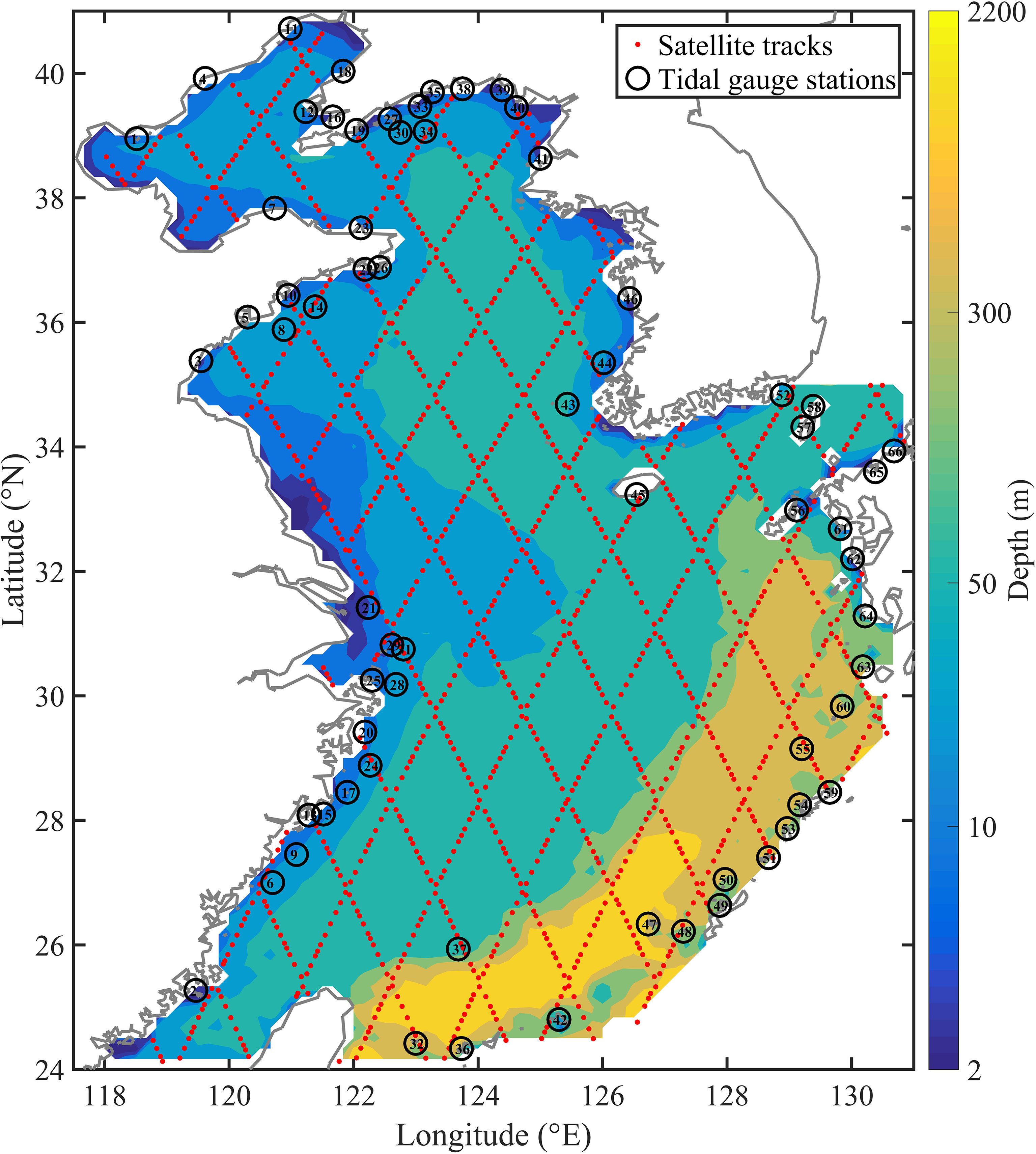
Figure 1 Bathymetric map of the BYECS (colors), and the positions of T/P satellite tracks (red points) and tidal gauge stations (black circles). The number in the black circles is the serial number of the tidal gauge stations in this study.

2.5 Model settings

The simulated area in this study was the BYECS (Figure 1), with a horizontal resolution of 10′×10′ and the time step of 80 s. The horizontal eddy viscosity coefficient A was set as a constant of 5000 m²/s (Wang et al., 2021b). Following Kang et al. (1998) and Wang et al. (2014), the default value of the Manning’s n coefficient was set to 0.023 s/m^1/3 (the unit was hereafter omitted by convention). Four principal tidal constituents M₂, S₂, K₁ and O₁ in the BYECS were simulated. Following Wang et al. (2021b), the 2D multi-constituent tidal model was run for 30 d from 1 January 2010 and the initial 15 d was spun up. The simulated results in the final 15 d were analysed to separate the simulated four principal tidal constituents (Cao et al., 2015). The adjoint model was run for 15 d backward in time from 31 January 2010 with the same horizontal resolution and time step.

3 Twin experiments

3.1 Experimental design

To test the effectiveness of the adjoint data assimilation in estimating the Manning’s n coefficient, several twin experiments were designed. In the twin experiments, the synthetic ‘observations’ are the simulated results at the spatial and temporal locations of the actual observations by running the numerical model with the prescribed ‘real’ model parameters. In this study, the ‘real’ Manning’s n coefficient was assumed to be 0.023 in the twin experiments. The 2D multi-constituent tidal model was run to simulate the four principal tidal constituents (M₂, S₂, K₁ and O₁) with the ‘real’ Manning’s n coefficient and the other default model settings as shown in Section 2.5. The simulated sea surface elevation at the spatial locations of the T/P satellite tracks (tidal gauge stations) were analysed. The obtained amplitudes and phase lags of the four principal tidal constituents M₂, S₂, K₁ and O₁ at the spatial locations of the T/P satellite tracks (tidal gauge stations) were taken as synthetic AOs (COs) in the following twin experiments. In all the twin experiments, the Manning’s n coefficient was assumed to be constant. In twin experiment TE11, the constant Manning’s n coefficient was estimated with the initial guess value of 0.0115, which was half of the prescribed ‘real’ Manning’s n coefficient, by assimilating the synthetic AOs. Given the measurement errors associated with observations, the synthetic AOs were contaminated by adding 10%-30% artificial random errors with uniform distribution in twin experiment TE12. In addition, the initial guess value of Manning’s n coefficient was 0.0115 in TE12. In twin experiment TE13 and TE14, model settings were mostly the same as those in TE12 except that the artificial random errors were set as 40%-60% and 70%-90%, respectively. As the artificial errors were randomly added into the synthetic AOs, 10 scenarios with different random seeds were performed in TE12-TE14 and the averaged results were taken as the final results of the corresponding twin experiment. To test the effect of different initial guess value, the constant Manning’s n coefficient was estimated in twin experiment TE21-TE24 with the initial guess value of 0.0345 that was 1.5 times of the prescribed ‘real’ Manning’s n coefficient. 10 scenarios were also performed in TE22-TE24 by assimilating the same synthetic AOs in the 10 scenarios in TE12-TE14, respectively. The other model settings of all the twin experiments were the same as those described in Section 2.3 and Section 2.5, and some detailed model settings of the twin experiments are listed in Table 1. The vectorial errors and mean vectorial errors between the synthetic AOs (COs) and the simulated harmonic constants in the twin experiments, calculated using Eq. (13), were used to evaluate the effect of data assimilation.

TABLE 1

Table 1 Detailed model settings of the numerical experiments.

3.2 Results

As listed in Table 2, the vectorial errors of tidal constituents M₂, S₂, K₁ and O₁ between the synthetic AOs and the corresponding simulated results in all the twin experiments are significantly reduced. The mean vectorial error for AOs before data assimilation is 7.16 cm in TE11-TE14. After data assimilation, the mean vectorial error for AOs is decreased to 0.37 cm in TE11, 0.43 cm in TE12, 1.99 cm in TE13 and 2.92 cm in TE14 (Table 2). The mean vectorial error for AOs is decreased from 5.18 cm before data assimilation to 0.42 cm in TE21, 0.45 cm in TE22, 1.37 cm in TE23 and 2.27 cm in TE24 (Table 2). The results show that the synthetic AOs in all the twin experiments are fully assimilated. Meanwhile, the L₁ norm of gradients of cost function with respect to the Manning’s n coefficient in all the scenarios in TE11-TE14 (Figure 2) and TE21-TE24 (Figure 3) are largely reduced and tend to be stable, indicating that the Manning’s n coefficients in all the twin experiments are adequately estimated.

TABLE 2

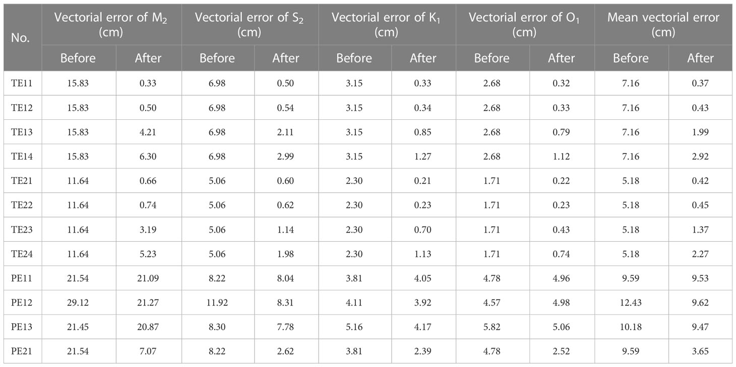
Table 2 Vectorial errors and mean vectorial error of the four principal tidal constituents between the AOs and the corresponding simulated results in the numerical experiments.

FIGURE 2

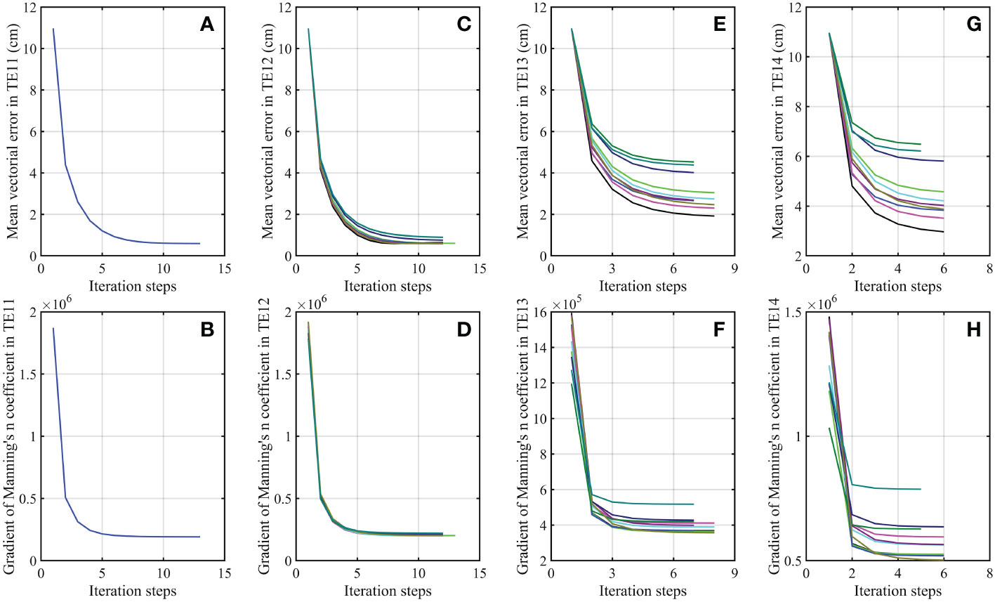
Figure 2 Variations of (A) the mean vectorial error of the four tidal constituents M₂, S₂, K₁ and O₁ for COs and (B) the L₁ norm of gradients of cost function with respect to the Manning’s n coefficient in TE11. (C, D) same as (A, B) but for TE12. (E, F) same as (A, B) but for TE13. (G, H) same as (A, B) but for TE14. The colored lines in (C–G) and (D–H) indicate the results in the 10 scenarios of the corresponding experiment.

FIGURE 3

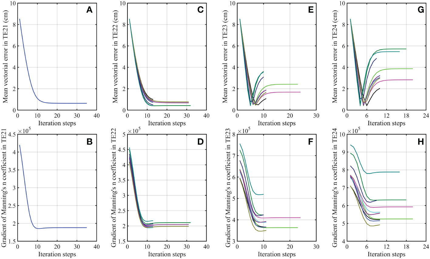
Figure 3 Same as Figure 2, but for (A, B) TE21, (C, D) TE22, (E, F) TE23 and (G, H) TE24.

The effect of the adjoint data assimilation in improving the simulation accuracy should be evaluated by the independent observations. As shown in Figure 2, the mean vectorial errors of the four principal tidal constituents between the synthetic COs and the corresponding simulated results in TE11-TE14 are gradually reduced and tend to be stable within 15 iteration steps. In addition, all the vectorial errors of M₂, S₂, K₁ and O₁ between the synthetic COs and the corresponding simulated results are largely decreased in TE11-TE14 (Table 3). The mean vectorial error for COs is reduced to 0.59 cm in TE11, 0.68 cm in TE12, 3.08 cm in TE13 and 4.55 cm in TE14 from an initial value of 10.97 cm (Table 3), indicating the model performance is improved with a reduction of 94.62%, 93.80%, 71.92% and 58.52% for the data misfit between the simulated results and independent observations in TE11, TE12, TE13 and TE14, respectively. As shown in Figures 3A, C, the mean vectorial errors for COs in TE21 and TE22 are gradually reduced and reach the minimum value within 35 iteration steps. Although the mean vectorial errors for COs in TE23 and TE24 are firstly reduced and then increased with the increase of iteration steps, the final results are still less than those before data assimilation, as shown in Figures 3E, G, respectively. As listed in Table 3, the vectorial errors of M₂, S₂, K₁ and O₁ for COs are significantly reduced in TE21-TE24, and the mean vectoral errors for COs are reduced by 92.50% in TE21, 91.91% in TE22, 73.27% in TE23 and 56.27% in TE24, respectively. The results evaluated by the independent COs show that the model performance of the 2D multi-constituent tidal model is significantly improved by assimilating the synthetic AOs, regardless of the initial guess value of the Manning’s n coefficient being less or larger than the prescribed ‘real’ value.

TABLE 3

Table 3 Vectorial errors and mean vectorial error of the four principal tidal constituents between the COs and the corresponding simulated results in the numerical experiments.

When the percentage of the artificial random observational errors becomes larger, the MAEs between the simulated harmonic constants (amplitudes and phase lags) and the synthetic COs for the four principal tidal constituents M₂, S₂, K₁ and O₁ are increased from TE11 (TE21) to TE14 (TE24), especially for TE13 (TE23) and TE14 (TE24), and the standard deviations of the 10 scenarios are also increased, as shown in Figures 4, 5). Meanwhile, the difference between the estimated and prescribed Manning’s n coefficient is increased from TE11 (TE21) to TE14 (TE24), and the dispersion of the finally optimized Manning’s n coefficient is also increased with the increased percentage of the artificial random observational errors, as shown in Figure 6. The vectorial errors of the four principal tidal constituents and the mean vectorial error in TE12 (TE22) are slightly larger than those in TE11 (TE21). In addition, the final estimated Manning’s n coefficient in TE11 (TE21) and TE12 (TE22) are 0.0234 (0.0231) and 0.0233 (0.0232) as shown in Figures 6A, B, E, F), respectively. The results indicate that the 10%-30% random observational errors have little influence on the adjoint data assimilation and the estimation of the Manning’s n coefficient. When the percentage of the artificial random observational errors increases to 40%-60% and 70%-90%, however, those vectorial errors are significantly increased with a nearly linear trend (Figures 4, 5) and the estimated Manning’s n coefficients become obviously deviate from the prescribed value (Figure 6). When the percentage of the artificial random observational error is 40%-60%, the contaminated synthetic observations are nearly 0.5 times or 1.5 times of the true values in the average sense. As a result, the mean vectorial error for COs after data assimilation in TE13 (TE23) is about 5.22 (3.56) times that in TE11 (TE21) and the estimated Manning’s n coefficient is only 0.0199 (0.0199) in TE13 (TE23). When the percentage of the artificial random observational error is 70%-90%, the contaminated synthetic observations are much deviated from the true observations, hence the mean vectorial error for COs is much larger and the estimated Manning’s n coefficient is further deviated from the prescribed value. The above results indicate that when the observational errors are within reasonable range, the Manning’s n coefficient can be successfully estimated and the model performance can be significantly improved by assimilating AOs with the adjoint data assimilation. When the observational errors are too large, although the results may not be perfect, the model performance can still be improved and the estimated Manning’s n coefficient can be much closer to the prescribed value than those before data assimilation.

FIGURE 4

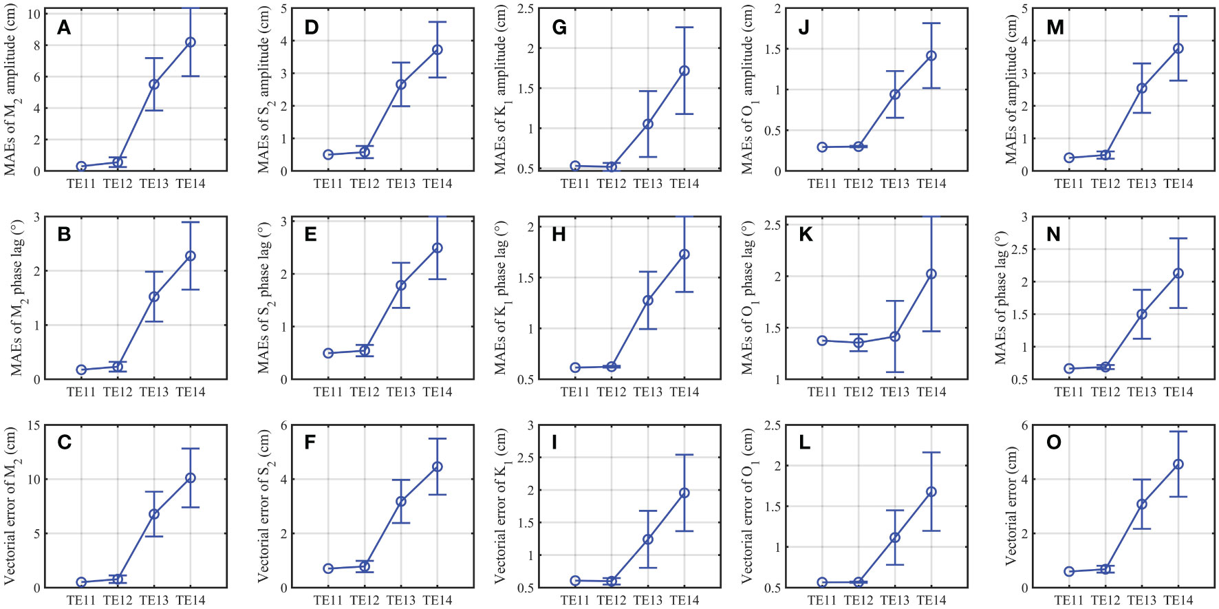
Figure 4 Variations of (A) MAEs of the M₂ amplitude between the COs and the corresponding simulated results in TE11, TE12, TE13 and TE14. (B, C) same as (A) but for MAEs of the M₂ phase lag and vectorial error of M₂, respectively. (D–F) same as (A–C) but for S₂. (G–I) same as (A–C) but for K₁. (J–L) same as (A–C) but for O₁. (M–O) same as (A–C) but for the averaged values of the above-mentioned four tidal constituents. Blue vertical bars indicate the standard deviation of the 10 scenarios in the corresponding experiment.

FIGURE 5

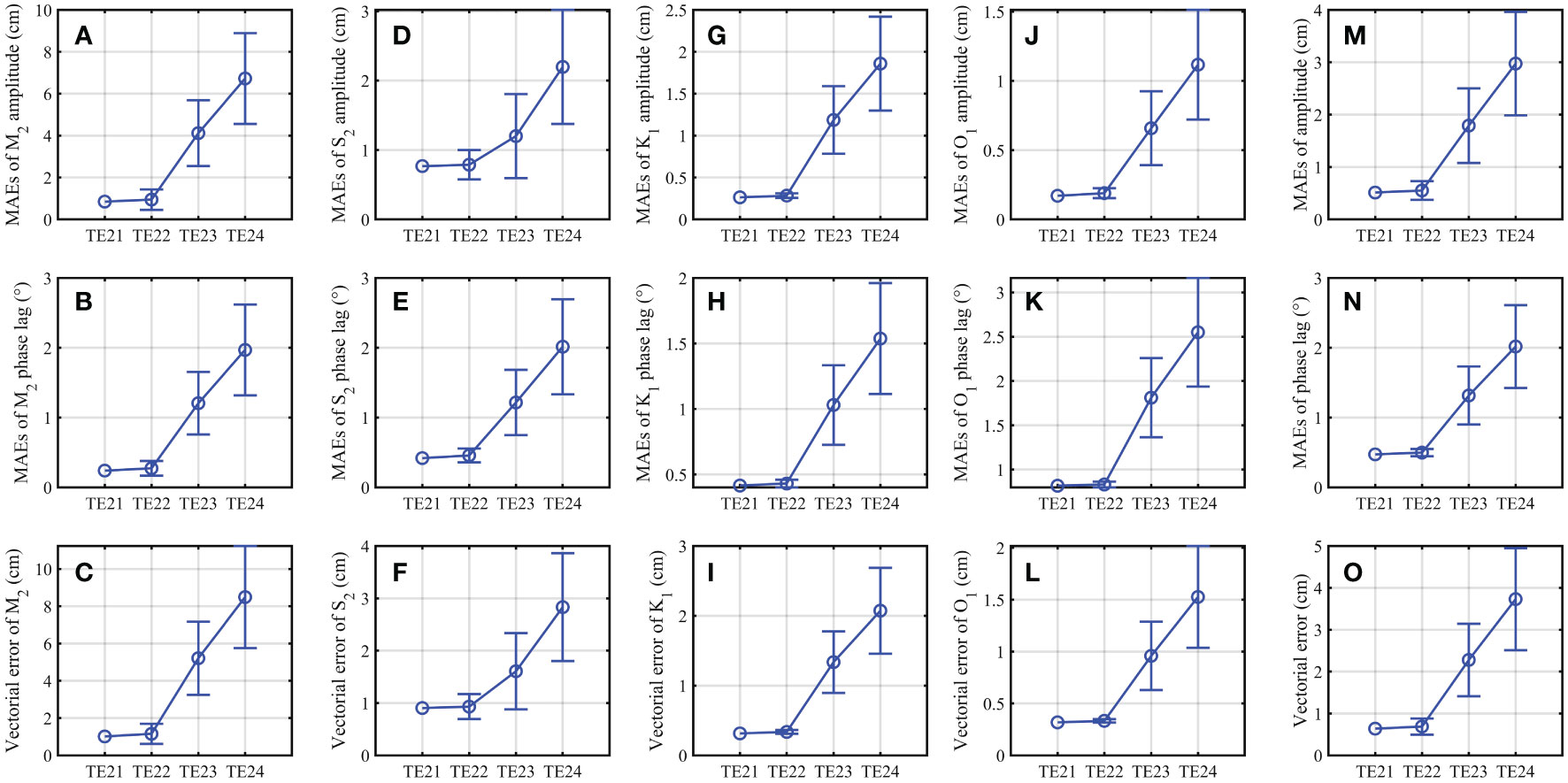
Figure 5 Variations of (A) MAEs of the M₂ amplitude between the COs and the corresponding simulated results in TE21, TE22, TE23 and TE24. (B, C) same as (A) but for MAEs of the M₂ phase lag and vectorial error of M₂, respectively. (D–F) same as (A–C) but for S₂. (G–I) same as (A–C) but for K₁. (J–L) same as (A–C) but for O₁. (M–O) same as (A–C) but for the averaged values of the above-mentioned four tidal constituents. Blue vertical bars indicate the standard deviation of the 10 scenarios in the corresponding experiment.

FIGURE 6

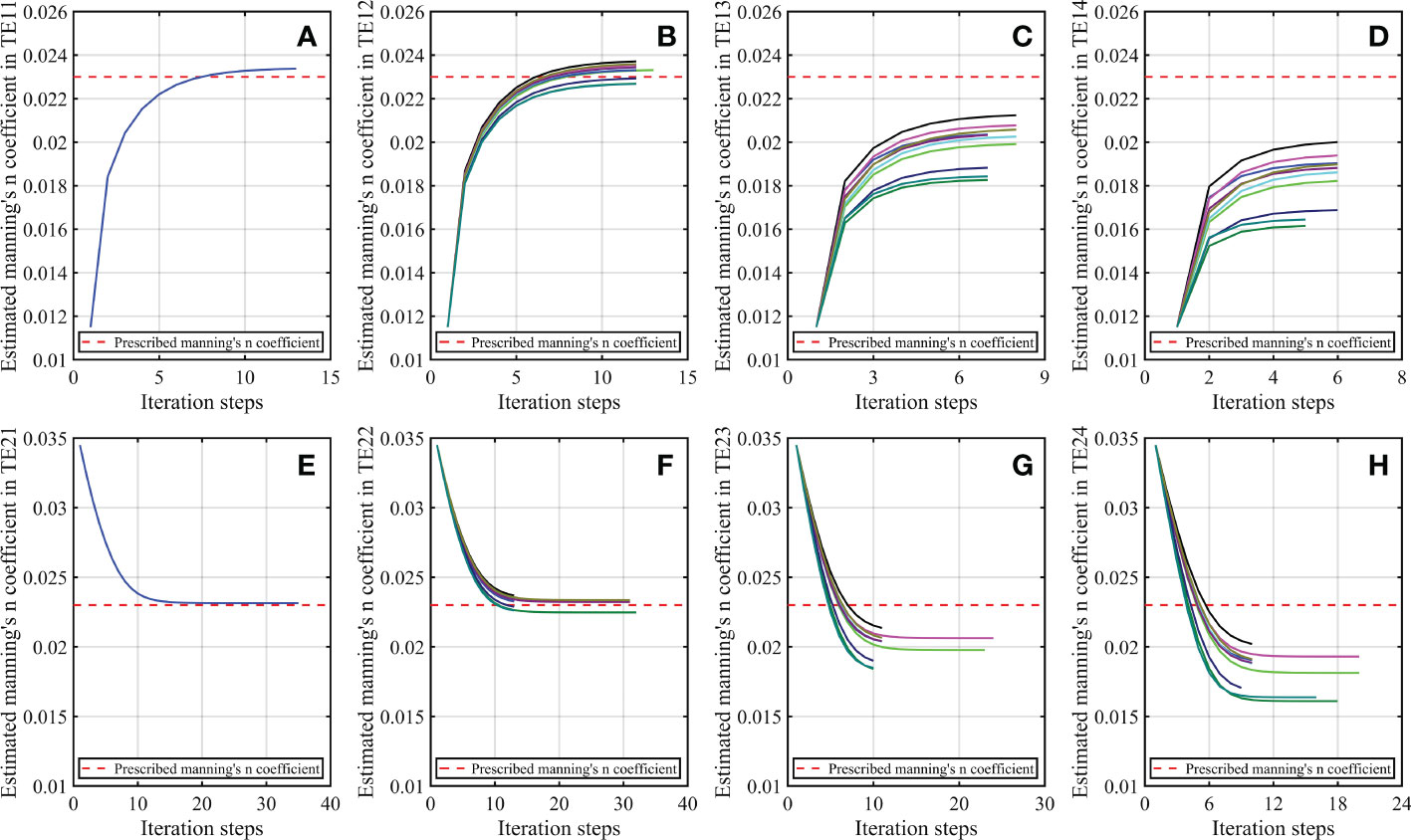
Figure 6 (A) Prescribed Manning’s n coefficient (red dashed line) and the estimated results (blue line) in TE11. (B) Prescribed Manning’s n coefficient (red dashed line) and the estimated results in the 10 scenarios (colored lines) in TE12. (C, D) same as (B) but for TE13 and TE14, respectively. (E–H) same as (A–D) but for TE21, TE22, TE23 and TE24, respectively.

Regardless of the inclusion of artificial random errors associated with synthetic AOs, the simulated four principal tidal constituents M₂, S₂, K₁ and O₁ after the data assimilation are consistently much closer to the COs than those before the data assimilation in all the twin experiments, demonstrating that the adjoint data assimilation can effectively improve the model performance. In addition, the estimated Manning’s n coefficient using the adjoint data assimilation is very close to the prescribed value when the observational errors are within reasonable range, no matter the initial guess value of the Manning’s n coefficient is less or larger than the prescribed value. Even if the observational errors are very large, the estimated Manning’s n coefficient is much closer to the prescribed value than the initial guess value. The results of the twin experiments demonstrate that the adjoint data assimilation can significantly improve simulation accuracy of the tide and is an effective method to estimate the Manning’s n coefficient in multi-constituent tidal models by assimilating reasonable observations.

4 Practical experiments

4.1 Experimental design

In the practical experiments, the actual AOs were assimilated to estimate the Manning’s n coefficient using the adjoint data assimilation. In PE11, the Manning’s n coefficient was assumed to be constant and the initial guess value was set to 0.023 that was generally used in the traditional numerical studies in the BYECS. In PE12 and PE13, the initial guess value of the Manning’s n coefficient was set to 0.5 and 1.5 times 0.023, respectively. The spatially varying Manning’s n coefficient was widely used in previous studies (Mayo et al., 2014; Demissie and Bacopoulos, 2017). Mohammadian et al. (2022) found that the calibrated Manning’s n coefficient on the ebb tide was nearly 60% of that on the flood tide in the Koksoak River Estuary, showing that the Manning’s n coefficient would be also temporally varying. Slivinski et al. (2017) found that the spatially varying Manning’s n coefficients estimated by assimilating the velocity observations in 2011 were no longer optimal in 2013, indicating the spatial and temporal variation of the Manning’s n coefficient. In order to further improve the model performance of the 2D multi-constituent tidal model, the Manning’s n coefficient was assumed to be spatially-temporally varying in PE21, in which the initial guess value of the Manning’s n coefficient was set to 0.023 that was used in PE11. The other model settings were the same as those described in Section 2.3 and Section 2.5, and some details are listed in Table 1.

4.2 Results

As shown in Figure 7, the normalized cost functions in all the practical experiments are gradually reduced and tend to be stable. The vectorial errors of M₂ and S₂ between the AOs and the corresponding simulated results after the data assimilation in all the practical experiments are less than those before data assimilation (Table 2). As listed in Table 2, the mean vectorial errors for AOs are reduced from 9.59 cm to 9.53 cm in PE11, from 12.43 cm to 9.62 cm in PE12, from 10.18 cm to 9.47 cm in PE13, from 9.59 cm to 3.65 cm in PE21. These considerable reductions indicate that the AOs are effectively assimilated. When the Manning’s n coefficient is assumed to be constant in PE11, the MAEs of M₂ tidal amplitude and phase lag and the vectorial error of M₂ between the COs and the simulated results are slightly reduced (Figures 8A–C), with similar pattern occurred to S₂ (Figures 8D–F). Although the MAEs of tidal amplitude and phase lag and the vectorial errors of K1 and O1 between the COs and the simulated results in PE11 are increased after data assimilation (Figures 8G–L), the mean vectoral error for COs in PE11 is reduced from 12.62 cm to 12.52 cm (Table 3), suggesting that the model performance is slightly improved in PE11. The vectoral errors of K₁ and O₁ between the COs and the corresponding simulated results in PE12 are firstly decreased and then increased to be slightly larger than that before data assimilation as shown in Figures 8I, L, so as to achieve smaller errors overall considering that the amplitudes of K₁ and O₁ are much less than those of M₂ and S₂ in the BYECS (Fang et al., 2004). The mean vectoral error for COs in PE12 is still largely reduced from 16.54 cm to 12.64 cm, which is close to 12.52 cm obtained in PE11 (Table 3). In addition, the mean vectorial error for COs after data assimilation in PE13 is 12.44 cm and also close to that obtained in PE11. Similarly, the estimated constant Manning’s n coefficient after data assimilation is 2.506×10^-2 in PE11, 2.503×10^-2 in PE12, and 2.546×10^-2 in PE13 (Figure 7D), which are close to each other. Overall, the aforementioned results show that regardless the initial guess value of the Manning’s n coefficient being too small or too large, the model performance can be effectively improved by the adjoint data assimilation. The Manning’s n coefficient can be successfully estimated and the optimal value is approximately 0.025 in the BYECS, which is nearly close to the averaged value of the globally optimized Manning’s n coefficients in this area in Blakely et al. (2022).

FIGURE 7

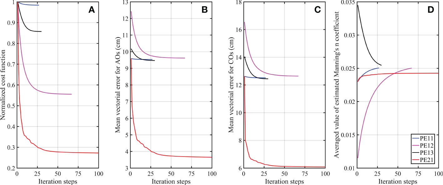
Figure 7 Variations of (A) the normalized cost function, (B) the mean vectorial error of the four tidal constituents M₂, S₂, K₁ and O₁ between the AOs and the simulated results, (C) the mean vectorial error of the four tidal constituents M₂, S₂, K₁ and O₁ between the COs and the simulated results, and (D) the spatially and temporally averaged value of the estimated Manning’s n coefficient, in PE11 (blue line), PE12 (magenta line), PE13 (black line) and PE21 (red line).

FIGURE 8

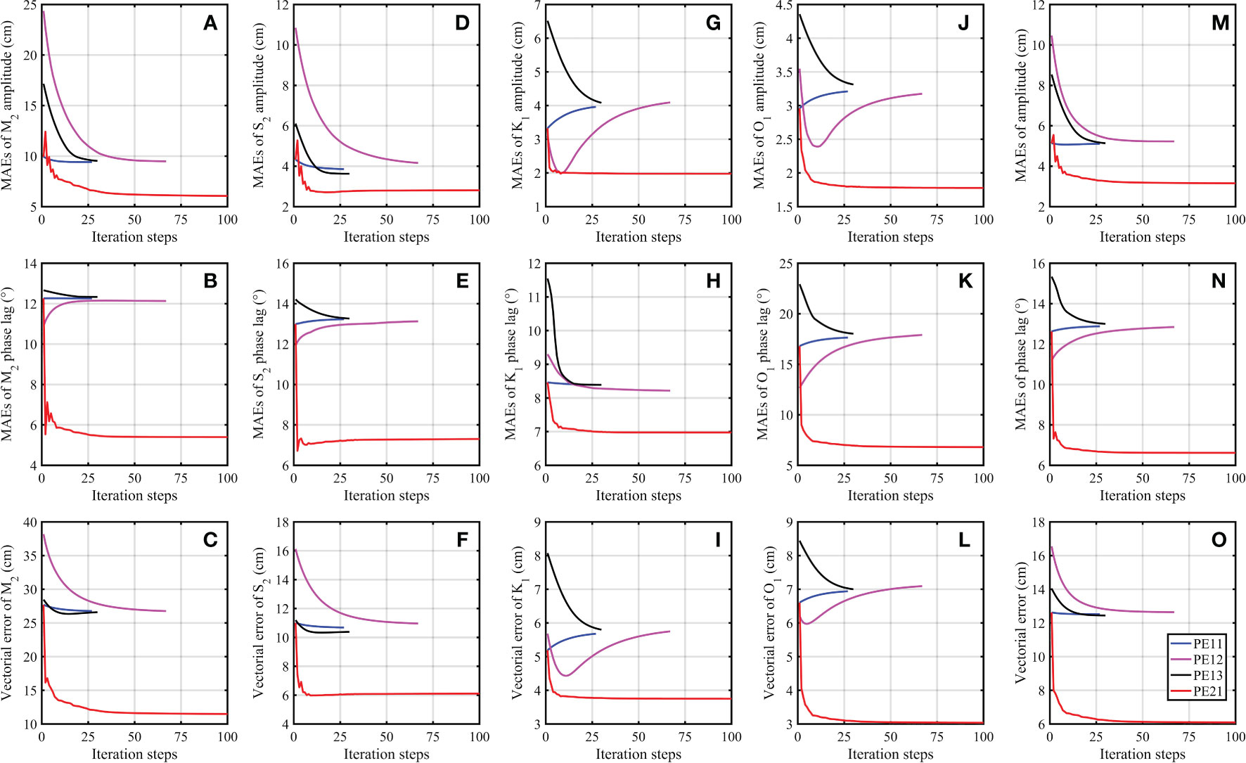
Figure 8 Variations of (A) MAEs of the M₂ amplitude between COs and the corresponding simulated results in PE11 (blue line), PE12 (magenta line), PE13 (black line) and PE21 (red line). (B, C) same as (A) but for MAEs of the M₂ phase lag and vectorial error of M₂, respectively. (D–F) same as (A–C) but for S₂. (G–I) same as (A–C) but for K₁. (J–L) same as (A–C) but for O₁. (M–O) same as (A–C) but for the averaged values of the above-mentioned four tidal constituents.

Although the model performance is improved by the adjoint data assimilation when the Manning’s n coefficient is assumed to be constant in PE11, PE12 and PE13, the mean vectorial errors after data assimilation with constant Manning’s n coefficient are much larger than the mean vectorial error of 6.90 cm obtained after data assimilation when the BFC is directly assumed to be spatially and temporally varying in Wang et al. (2021b). The Manning’s n coefficient has been confirmed to be spatially-temporally varying (Slivinski et al., 2017), so the spatially-temporally varying Manning’s n coefficient was estimated in PE21. As shown in Figure 7, the normalized cost function and the mean vectorial error for AOs in PE21 are significantly decreased and the values after data assimilation are much less than those in PE11, PE12 and PE13, indicating that the AOs are fully assimilated. As shown in Figure 8, the MAEs of the amplitude and phase lag of the four principal tidal constituents between the COs and the corresponding simulated results after data assimilation in PE21 are much less than those before data assimilation in PE21 and those after data assimilation in PE11, PE12 and PE13. In addition, the vectoral error between the COs and the corresponding simulated results in PE21 is reduced to 11.48 cm for M₂, 6.10 cm for S₂, 3.75 cm for K₁ and 3.04 cm for O₁ (Table 3), which are much less than those in PE11, PE12 and PE13. The mean vectorial error of the four tidal constituents between the COs and the corresponding simulated results in PE21 is reduced to 6.09 cm from an initial value of 12.62 cm (Table 3), indicating that the model performance is improved with a reduction of 51.74% for the difference between the independent observations without assimilated and the simulated results. The percentage of the reduction is nearly 65.3 times that in PE11. Moreover, the mean vectorial error for COs after data assimilation in PE21 is just 6.09 cm and less than the value of 6.90 cm in Wang et al. (2021b) in which the same four tidal constituents were simulated by assimilating the same AOs in the BYECS. As shown in Figure 9, the mean vectorial errors of the four principal tidal constituents for COs in PE21 at No. 3 and No. 21 tidal gauge stations, located at the central western boundary of the BYECS (Figure 1), are larger than those at other practical experiments, possibly because of the low resolution of bathymetry data or the low observation accuracy of T/P satellite altimeter data in this area. In addition, the mean vectorial errors for COs in PE21 at the stations near the southern and eastern open boundary with the serial number of 36, 42, 47, 48, 49, 52, 54, 55 and 62 (Figure 1) are slightly larger than those at the other practical experiments. At the other 55 tidal gauge stations other than those already mentioned, the mean vectorial errors for COs in PE21 are significantly less than those in PE11, PE12 and PE13, especially for the stations with the serial number less than 47. Model performance is obviously improved at most area in the BYECS by estimating the spatially-temporally varying Manning’s n coefficient with the adjoint data assimilation.

FIGURE 9

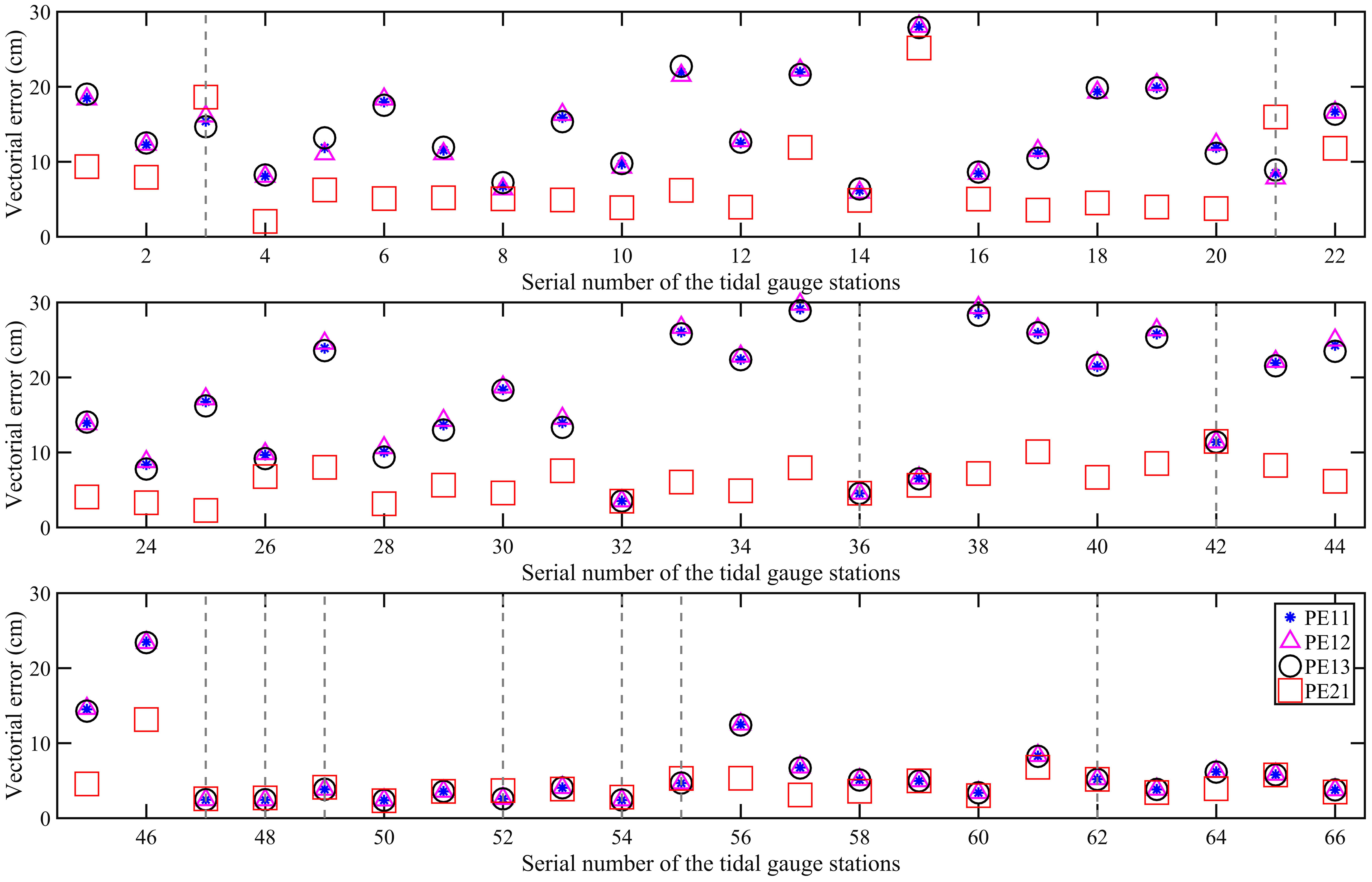
Figure 9 The mean vectorial error of the four tidal constituents between the COs and the corresponding simulated results in PE11 (blue asterisk), PE12 (magenta triangle), PE13 (black circle) and PE21 (red square) at all the tidal gauge stations. The gray dashed line shows that the mean vectorial error in PE21 at this tidal gauge station is larger than that in either of the other three experiments.

Besides a few special observational stations, the model after data assimilation in PE21 captures almost all (no less than 97%) of both the observed amplitude and phase lag of the four tidal constituents in AOs and COs with a factor of 2 (Supplementary Figure 1). In addition, the correlation coefficients of the observed and simulated tidal harmonic constants are not less than 0.90, indicating that the model is reasonably accurate even though only the observations retrieved from the T/P satellite altimeter data are assimilated in the BYECS. Furthermore, both the cotidal charts (Supplementary Figure 2) and the tidal current ellipses (Supplementary Figure 3) of the four principal tidal constituents M₂, S₂, K₁ and O₁ obtained in PE21 show the same patterns as those in the previous studies (Fang, 1994; Guo and Yanagi, 1998; Fang et al., 2004; Wang et al., 2021b), indicating that the simulated results after data assimilation are adequate enough to show the tidal characteristics in the BYECS and the Manning’s n coefficient is reasonably estimated with the assumption of spatial and temporal variations.

Overall, the aforementioned results indicate that under both scenarios of the constant and spatially-temporally varying Manning’s n coefficient in the practical experiments, the model performance can be improved by estimating the Manning’s n coefficient with the adjoint data assimilation, as evaluated by the difference between the independent observations of tidal harmonic constants (amplitude and phase lag) and the corresponding simulated results. When the Manning’s n coefficient is assumed to be spatially-temporally varying, the model performance can be significantly improved with a reduction of 51.74% for the difference between the independent observations without assimilated and the simulated results, showing that the Manning’s n coefficient in multi-constituent tidal models can be reasonably estimated by assimilating satellite observations with the adjoint data assimilation.

5 Discussions

5.1 Spatial distribution and temporal variation of the estimated Manning’s n coefficient

As indicated by Wang et al. (2018) and Wang et al. (2021b), the spatially-temporally varying model parameters estimated by the adjoint data assimilation may be affected by the model settings and should be discussed by the sensitivity experiments using the local forward sensitivity analysis (Zou et al., 1993a; Cacuci, 2003). Therefore, several sensitivity experiments were carried out to test the robustness of the spatially-temporally varying Manning’s n coefficient estimated in PE21. In the sensitivity experiment SE1 (SE2), the initial guess value of the Manning’s n coefficient was set to 0.5 (1.5) times 0.023 that used in PE21 to test the influence of the initial guess value in the adjoint data assimilation. In the sensitivity experiment SE3 (SE4), the step size used in the estimation of the Manning’s n coefficient in Eq. (12) was set to 0.5 (1.5) times that used in PE21 to test the influence of the adjustment strategy. Only M₂ and K₁ were simulated in the sensitivity experiment SE5 and only M₂ was simulated in the sensitivity experiment SE6, to test the influence of the number of the simulated tidal constituents. In the sensitivity experiment SE7, the starting time of the numerical experiment was set to 16 January 2010 to test the influence of the simulated period. The typical model settings of the sensitivity experiments are listed in Table 4, and the other model settings were the same as those in PE21.

TABLE 4

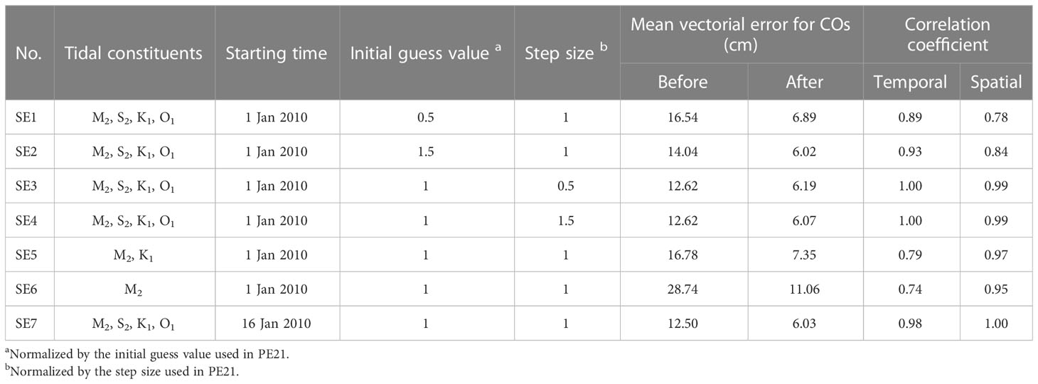
Table 4 Detailed model settings and results of the sensitivity experiments.

As listed in Table 4, the mean vectorial errors for COs in all the sensitivity experiments are substantially decreased, showing that the AOs are fully assimilated and the model performance is effectively improved. To evaluate the influence of the model settings on the estimated results, the spatially-temporally varying Manning’s n coefficient estimated by the adjoint data assimilation in PE21 and all the sensitivity experiments are temporally (spatially) averaged to get the spatial distribution (temporal variation) of the Manning’s n coefficient. The correlation coefficients between the temporal variation of the estimated Manning’s n coefficient in PE21 and those in the sensitivity experiments are not less than 0.74 (Table 4), suggesting a significant positive correlation at the 0.1 percent confidence level. Except for SE5 and SE6, the correlation coefficients were not less than 0.89. The correlation coefficients for the spatial distributions were not less than 0.78 in all the sensitivity experiments, indicating a significant positive correlation at the 0.1 percent confidence level. The results show that the trend of the spatially-temporally varying Manning’s n coefficient estimated in PE21 is not affected by the model settings and is relatively robust.

The simulated sea surface elevation and the estimated Manning’s n coefficient are spatially averaged to obtain the temporal variation. As shown in Figures 10A, B, the temporally varying sea surface elevation simulated in PE21 varies semi-diurnally and diurnally, while the variation period of the temporally varying Manning’s n coefficient estimated in PE21 is quarter-diurnal and one-third diurnal. The correlation coefficient between the temporally varying sea surface elevation and Manning’s n coefficient in PE21 is only -0.02. The temporally varying Manning’s n coefficient and current speed in PE21 have the similar variation period (Figures 10C, D) and the correlation coefficient is -0.43, indicating that the temporally varying Manning’s n coefficient is related to the current speed. When only M₂ and K₁ are simulated in SE5, the temporal variations of the Manning’s n coefficient and current speed become slightly simple (Figures 10E, F), and the correlation coefficient is -0.46. When only M₂ is simulated in SE6, both the estimated Manning’s n coefficient and current speed vary quarter-diurnally (Figures 10G, H), and the correlation coefficient is -0.56. The above results show that the temporal variation of the spatially averaged Manning’s n coefficient estimated by the adjoint data assimilation is negatively correlated with the current speed on the whole.

FIGURE 10

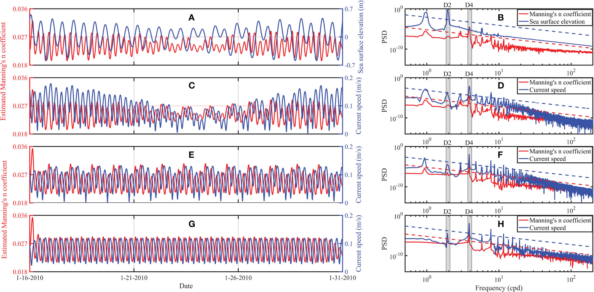
Figure 10 (A) Time series of the spatially averaged Manning’s n coefficient (red line) and sea surface elevation (blue line) in PE21, (B) power spectral densities of the spatially averaged Manning’s n coefficient (red line) and sea surface elevation (blue line) in PE21. (C, D) Same as (A, B) but for the spatially averaged Manning’s n coefficient (red line) and current speed (blue line) in PE21. (E, F) Same as (C, D) but for SE5. (G, H) Same as (C, D) but for SE6.

The estimated Manning’s n coefficient in PE21 is temporally averaged to obtain the spatial distribution (Figure 11). The spatial distribution of the Manning’s n coefficient is larger than 0.04 near the coastline of the BYECS, as shown in Figure 11A. The temporally averaged Manning’s n coefficient near the coastline of the Bohai Sea is much larger than that in the central area of the Bohai Sea, as shown in Figure 11B, which is consistent with that the estimation of the Manning’s n coefficient should be focused on the shallow areas (Mayo et al., 2014). Manning’s n formulation (Eq. (4)) suggests that the Manning’s n coefficient will have less effect on the simulated results for the large water depth. As a result, the temporally averaged Manning’s n coefficient is close to the initial guess value of 0.023 in most areas with water depth larger than 30 m. The temporally averaged Manning’s n coefficient is less than 0.002 near the Yangtze Estuary (Figure 11C), and the area is close to the mud area off the Yangtze Estuary where the sea bed is composed of fine sediment and the bed surface is smooth (Bian et al., 2013). In the Hangzhou Bay with rapid tidal current (Supplementary Figure 3), the temporally averaged Manning’s n coefficient is large, because the high tidal current tends to resuspend the fine sediments leaving a rougher surface or create ripples and dunes on the seabed (Blakely et al., 2022). In the middle of the BYECS with the centre of 126°E and 30°N, the estimated Manning’s n coefficient is larger than 0.03, which may be related to the spatial distribution of sand there as shown in Dutkiewicz et al. (2015). In some areas, the estimated Manning’s n coefficient may be not exactly correlated with the physical characteristics, which may be related to the low resolution of bathymetry data or the low observation accuracy of T/P satellite altimeter data in some area. Overall, the estimated Manning’s n coefficient in PE21 shows significant spatial variation in the shallow water areas.

FIGURE 11

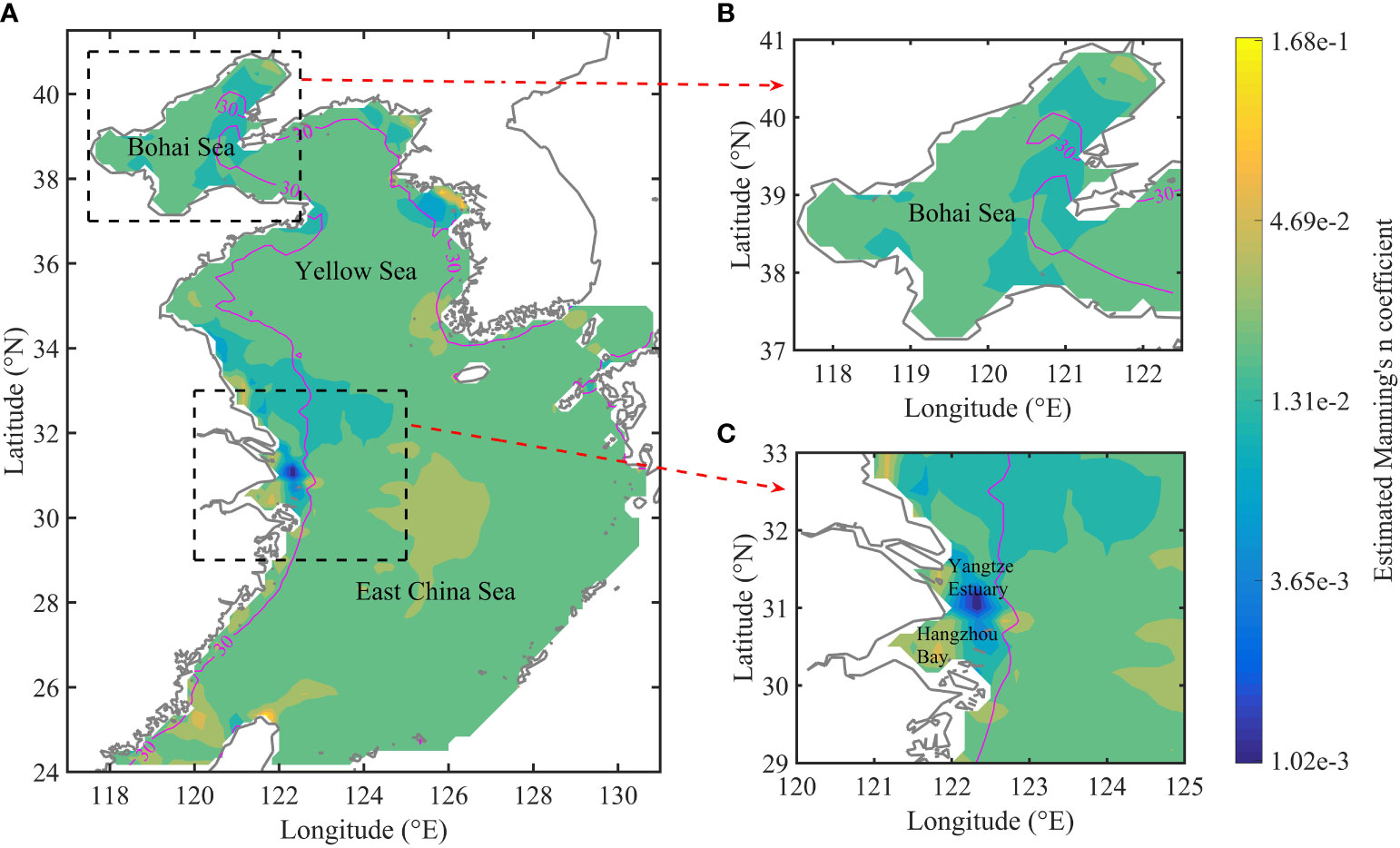
Figure 11 Spatial distribution of the temporally averaged Manning’s n coefficient in (A) the BYECS, (B) the Bohai Sea and (C) the Yangtze Estuary and the Hangzhou Bay, in PE21. The magenta line shows the bathymetric contours at 30 m.

5.2 Settings of the Manning’s n coefficient in tidal models

As discussed by Wang et al. (2021b), the Manning’s n formulation has been widely used in tidal models and the Manning’s n coefficient should be accurately determined. As shown in the practical experiments PE12 and PE13, when the Manning’s n coefficient is set to unreasonable constant value, the errors between the observations and the simulated results are large (Table 3). However, when the adjoint data assimilated is used to estimate the constant Manning’s n coefficient by assimilating the publicly available satellite observations, the errors can be considerably reduced (Figure 7C) and the estimated Manning’s n coefficient will tend to be the similar optimal value (Figure 7D). For the 2D multi-constituent tidal model used in this study, the optimal value of the constant Manning’s n coefficient is approximately 0.025 in the BYECS, which is suggested to the other tidal models using the constant Manning’s n coefficient in the BYECS. Although the optimal value of 0.025 is nearly close to the averaged value of the globally optimized Manning’s n coefficients in this area in Blakely et al. (2022), it is greater than the locally re-optimized Manning’s n coefficients in this area in Blakely et al. (2022). Therefore, when the internal tide dissipation is considered in the tidal model, it is necessary to simultaneously estimate the Manning’s n coefficient and the internal tide dissipation coefficient using the adjoint data assimilation, which will be the future work.

As shown by the twin experiments, the observational errors are important to estimate accuracy of the Manning’s n coefficient using the adjoint data assimilation. When the mean percentage of the observational errors reaches 50%, the estimated Manning’s n coefficients in both TE13 and TE23 are far deviated from the prescribed ‘real’ value. With the development of satellite remote sensing observational technology, the accuracy of the satellite observations is markedly improved. The accuracy of the observed amplitudes and phase lags by the T/P satellite altimeter data are about 2-4 cm and 5° in the BYECS (Fang et al., 2004), respectively, indicating that the publicly available satellite observations of the sea level are adequate enough for estimating the Manning’s n coefficient in the coastal tidal models. However, when the Manning’s n coefficient is assumed to be constant in PE11-PE13, only slight improvement exists for 2D multi-constituent tidal model in the BYECS, so it is necessary to set the spatially or temporally varying Manning’s n coefficient. Slivinski et al. (2017) found that the spatially varying Manning’s n coefficients estimated in 2011 were no longer optimal in 2013, indicating the spatial-temporal variation of the Manning’s n coefficient due to the changes of the geometry or bottom roughness (Sraj et al., 2014; Slivinski et al., 2017). When the Manning’s n coefficient is assumed to be spatially-temporally varying and estimated by the adjoint data assimilation in PE21, the mean vectorial error of the four tidal constituents is significantly decreased and the estimated spatially-temporally varying Manning’s n coefficient is robust. But it is difficult to propose a universal scheme to set the spatially-temporally varying Manning’s n coefficient in the tidal model at this stage. As well known, the Manning’s n coefficient is associated with the subaqueous land classifications (Bunya et al., 2010) and the theoretical Manning’s n coefficient can be determined according to the median grain size of the sediment of the seafloor (Warder et al., 2022). Therefore, it would be an important future research to establish a universal empirical formula of the Manning’s n coefficient considering the relationship between the Manning’s n coefficient and sediment type at seafloor. In addition, the unknown coefficients in this formula are further estimated by assimilating the observations with the adjoint data assimilation.

6 Conclusions

Tide is a ubiquitous oceanographic phenomenon in the global ocean (Wei et al., 2022) and is essential for the design and plan of coastal ocean engineering (Lee and Jeng, 2002; Chen et al., 2007; Wang et al., 2021a). The bottom friction is critical for the dissipation of the global tidal energy and is a quadratic function of BFC and velocity (Taylor, 1920). BFC is traditionally determined using the Manning’s n formulation in tidal models. So, the Manning’s n coefficient in the Manning’s n formulation is vital for the accurate simulation and prediction of the tide in shallow coastal waters, whereas it cannot be directly measured and contains large amounts of uncertainties. Based on a two-dimensional multi-constituent tidal model with the adjoint data assimilation developed in Wang et al. (2021b), the Manning’s n coefficient is estimated by assimilating satellite observations using the adjoint data assimilation in the BYECS with the simulation of four principal tidal constituents M₂, S₂, K₁ and O₁. The observed amplitudes and phase lags of the four principal tidal constituents retrieved from the satellite altimeter data are taken as AOs, while those at the tidal gauge stations are taken as COs to evaluate the simulation results.

In the twin experiments, the synthetic observations at the spatial locations of the satellite tracks are assimilated to estimate the constant Manning’s n coefficient. Regardless the inclusion of the artificial random observational errors associated with synthetic AOs, the simulated four principal tidal constituents M₂, S₂, K₁ and O₁ after the data assimilation are consistently much closer to the COs than those before the data assimilation in all the twin experiments (Table 3 and Figures 2, 3). In addition, the estimated Manning’s n coefficient is close to the prescribed value, especially when the percentage of the observational errors are not too large, no matter the initial guess value of the Manning’s n coefficient in the adjoint data assimilation is less or larger than the prescribed value (Figure 6). The results of the twin experiments demonstrate that the adjoint data assimilation can significantly improve simulation accuracy of the tide and is an effective method to estimate the Manning’s n coefficient.

In the practical experiments, under both scenarios of the constant and spatially-temporally varying Manning’s n coefficient, the model performance can be effectively improved by assimilating the satellite observations with the adjoint data assimilation. When the Manning’s n coefficient is assumed to be spatially-temporally varying, the model performance can be significantly improved with a reduction of 51.74% for the difference between COs and the simulated results (Table 3), showing that the Manning’s n coefficient in multi-constituent tidal models can be reasonably estimated by assimilating satellite observations with the adjoint data assimilation. In addition, the estimated spatial-temporal variation characteristics is robust and not affected by the model settings (Table 4). The spatially-temporally varying Manning’s n coefficient is negatively correlated with the current speed and show significant spatial variation on shallow areas.

This study demonstrate that the Manning’s n coefficient can be reasonably estimated by the adjoint data assimilation, which allows significant improvement in accurate simulation of the ocean tide. In the future, it is essential to propose a universal empirical formula of the Manning’s n coefficient considering the relationship between the Manning’s n coefficient and sediment type at seafloor. In addition, the unknown coefficients in this empirical formula should be estimated by assimilating the observations with the adjoint data assimilation, to further provide suggestions for setting the spatially-temporally varying Manning’s n coefficient in tidal models. Besides, it is also the future work to consider both the bottom boundary layer dissipation and the internal tide dissipation in the tidal model, and simultaneously estimate the Manning’s n coefficient and the internal tide dissipation coefficient using the adjoint data assimilation.

Data availability statement

The original contributions presented in the study are included in the article/Supplementary Material. Further inquiries can be directed to the corresponding author.

Author contributions

DW and JJ designed the original ideas. DW performed the numerical experiments and analyses. JJ, ZW, JC, and JZ contributed to the concept of the manuscript. DW wrote the original manuscript, JJ, JC, JZ, and ZW revised and improved the manuscript. All authors contributed to the article and approved the submitted version.

Funding

This study is jointly supported by Open Funds for Key Laboratory of Marine Environmental Survey Technology and Application, Ministry of Natural Resources (No. MESTA-2021-A004); Guangdong Basic and Applied Basic Research Foundation (No. 2023A1515011262, 2020A1515110339); National Key Research and Development Plan of China (No. 2022YFC2808304); National Natural Science Foundation of China (No. 42106033, 42176172, 41876086); Youth Foundation of Hubei University of Economics (No. XJ20BS46).

Conflict of interest

The authors declare that the research was conducted in the absence of any commercial or financial relationships that could be construed as a potential conflict of interest.

Publisher’s note

All claims expressed in this article are solely those of the authors and do not necessarily represent those of their affiliated organizations, or those of the publisher, the editors and the reviewers. Any product that may be evaluated in this article, or claim that may be made by its manufacturer, is not guaranteed or endorsed by the publisher.

Supplementary material

The Supplementary Material for this article can be found online at: https://www.frontiersin.org/articles/10.3389/fmars.2023.1151951/full#supplementary-material

References

Alekseev A., Navon I. M., Steward J. (2009). Comparison of advanced large-scale minimization algorithms for the solution of inverse ill-posed problems. Optimization Methods Softw. 24 (1), 63–87. doi: 10.1080/10556780802370746

CrossRef Full Text | Google Scholar

Bian C., Jiang W., Greatbatch R. J. (2013). An exploratory model study of sediment transport sources and deposits in the bohai Sea, yellow Sea, and East China Sea. J. Geophys. Research: Oceans 118 (11), 5908–5923. doi: 10.1002/2013JC009116

CrossRef Full Text | Google Scholar

Blakely C. P., Ling G., Pringle W. J., Contreras M. T., Wirasaet D., Westerink J. J., et al. (2022). Dissipation and bathymetric sensitivities in an unstructured mesh global tidal model. J. Geophys. Research: Oceans 127 (5), e2021JC018178. doi: 10.1029/2021JC018178

CrossRef Full Text | Google Scholar

Budgell W. (1987). Stochastic filtering of linear shallow water wave processes. SIAM J. Sci. Stat. Computing 8 (2), 152–170. doi: 10.1137/0908027

CrossRef Full Text | Google Scholar

Bunya S., Dietrich J. C., Westerink J., Ebersole B., Smith J., Atkinson J., et al. (2010). A high-resolution coupled riverine flow, tide, wind, wind wave, and storm surge model for southern Louisiana and mississippi. part I: Model development and validation. Monthly Weather Rev. 138 (2), 345–377. doi: 10.1175/2009MWR2906.1

CrossRef Full Text | Google Scholar

Cacuci D. G. (2003). Sensitivity and uncertainty analysis, volume I: theory (Boca Raton, Florida: CRC press).

Google Scholar

Cao A., Wang D., Lv X. (2015). Harmonic analysis in the simulation of multiple constituents: determination of the optimum length of time series. J. Atmospheric Oceanic Technol. 32 (5), 1112–1118. doi: 10.1175/JTECH-D-14-00148.1

CrossRef Full Text | Google Scholar

Chen B.-F., Wang H.-D., Chu C.-C. (2007). Wavelet and artificial neural network analyses of tide forecasting and supplement of tides around Taiwan and south China Sea. Ocean Eng. 34 (16), 2161–2175. doi: 10.1016/j.oceaneng.2007.04.003

CrossRef Full Text | Google Scholar

Demissie H. K., Bacopoulos P. (2017). Parameter estimation of anisotropic manning’s n coefficient for advanced circulation (ADCIRC) modeling of estuarine river currents (lower st. johns river). J. Mar. Syst. 169, 1–10. doi: 10.1016/j.jmarsys.2017.01.008

CrossRef Full Text | Google Scholar

Ding Y., Wang S. S. (2005). Identification of manning’s roughness coefficients in channel network using adjoint analysis. Int. J. Comput. Fluid Dynamics 19 (1), 3–13. doi: 10.1080/10618560410001710496

CrossRef Full Text | Google Scholar

Du Y., Wang D., Zhang J., Wang Y. P., Fan D. (2021). Estimation of initial conditions for surface suspended sediment simulations with the adjoint method: A case study in hangzhou bay. Continental Shelf Res. 227, 104526. doi: 10.1016/j.csr.2021.104526

CrossRef Full Text | Google Scholar

Dutkiewicz A., Müller R. D., O’Callaghan S., Jónasson H. (2015). Census of seafloor sediments in the world’s ocean. Geology 43 (9), 795–798. doi: 10.1130/G36883.1

CrossRef Full Text | Google Scholar

Egbert G. D., Erofeeva S. Y. (2002). Efficient inverse modeling of barotropic ocean tides. J. Atmospheric Oceanic Technol. 19 (2), 183–204. doi: 10.1175/1520-0426(2002)019<0183:eimobo>2.0.co;2

CrossRef Full Text | Google Scholar

Fan R., Zhao L., Lu Y., Nie H., Wei H. (2019). Impacts of currents and waves on bottom drag coefficient in the East China shelf seas. J. Geophys. Research: Oceans 124 (11), 7344–7354. doi: 10.1029/2019JC015097

CrossRef Full Text | Google Scholar

Fang G. (1994). “Tides and tidal currents in East China Sea, huanghai Sea and bohai Sea,” in Oceanology of China seas, vol. 101-112 . Eds. Zhou D., Liang Y.-B., Zeng C.-K. (Dordrecht: Springer).

Google Scholar

Fang G., Wang Y., Wei Z., Choi B. H., Wang X., Wang J. (2004). Empirical cotidal charts of the bohai, yellow, and East China seas from 10 years of TOPEX/Poseidon altimetry. J. Geophys. Research: Oceans 109, C11006. doi: 10.1029/2004JC002484

CrossRef Full Text | Google Scholar

Fringer O. B., Dawson C. N., He R., Ralston D. K., Zhang Y. J. (2019). The future of coastal and estuarine modeling: Findings from a workshop. Ocean Model. 143, 101458. doi: 10.1016/j.ocemod.2019.101458

CrossRef Full Text | Google Scholar

Gao X., Wei Z., Lv X., Wang Y., Fang G. (2015). Numerical study of tidal dynamics in the south China Sea with adjoint method. Ocean Model. 92, 101–114. doi: 10.1016/j.ocemod.2015.05.010

CrossRef Full Text | Google Scholar

Graham L., Butler T., Walsh S., Dawson C., Westerink J. J. (2017). A measure-theoretic algorithm for estimating bottom friction in a coastal inlet: Case study of bay st. Louis during hurricane Gustav, (2008). Monthly Weather Rev. 145 (3), 929–954. doi: 10.1175/MWR-D-16-0149.1

CrossRef Full Text | Google Scholar

Guo X., Yanagi T. (1998). Three-dimensional structure of tidal current in the East China Sea and the yellow Sea. J. Oceanogr. 54 (6), 651–668. doi: 10.1007/BF02823285

CrossRef Full Text | Google Scholar

Heemink A., Mouthaan E., Roest M., Vollebregt E., Robaczewska K., Verlaan M. (2002). Inverse 3D shallow water flow modelling of the continental shelf. Continental Shelf Res. 22 (3), 465–484. doi: 10.1016/S0278-4343(01)00071-1

CrossRef Full Text | Google Scholar

Hostache R., Lai X., Monnier J., Puech C. (2010). Assimilation of spatially distributed water levels into a shallow-water flood model. part II: Use of a remote sensing image of mosel river. J. Hydrol. 390 (3-4), 257–268. doi: 10.1016/j.jhydrol.2010.07.003

CrossRef Full Text | Google Scholar

Kang S. K., Lee S.-R., Lie H.-J. (1998). Fine grid tidal modeling of the yellow and East China seas. Continental Shelf Res. 18 (7), 739–772. doi: 10.1016/S0278-4343(98)00014-4

CrossRef Full Text | Google Scholar

Lee T. L., Jeng D. S. (2002). Application of artificial neural networks in tide-forecasting. Ocean Eng. 29 (9), 1003–1022. doi: 10.1016/S0029-8018(01)00068-3

CrossRef Full Text | Google Scholar

Lu X., Zhang J. (2006). Numerical study on spatially varying bottom friction coefficient of a 2D tidal model with adjoint method. Continental Shelf Res. 26 (16), 1905–1923. doi: 10.1016/j.csr.2006.06.007

CrossRef Full Text | Google Scholar

Mayo T., Butler T., Dawson C., Hoteit I. (2014). Data assimilation within the advanced circulation (ADCIRC) modeling framework for the estimation of manning’s friction coefficient. Ocean Model. 76, 43–58. doi: 10.1016/j.ocemod.2014.01.001

CrossRef Full Text | Google Scholar

Mohammadian A., Morse B., Robert J.-L. (2022). Calibration of a 3D hydrodynamic model for a hypertidal estuary with complex irregular bathymetry using adaptive parametrization of bottom roughness and eddy viscosity. Estuar. Coast. Shelf Sci. 265, 107655. doi: 10.1016/j.ecss.2021.107655

CrossRef Full Text | Google Scholar

Munk W., Wunsch C. (1998). Abyssal recipes II: Energetics of tidal and wind mixing. Deep-sea research. Part I Oceanogr. Res. Papers 45 (12), 1977–2010. doi: 10.1016/S0967-0637(98)00070-3

CrossRef Full Text | Google Scholar

Navon I. M. (1998). Practical and theoretical aspects of adjoint parameter estimation and identifiability in meteorology and oceanography. Dynamics of Atmospheres and Oceans, (Special issue in honor of Richard pfeffer) 27, 55–79.

Google Scholar

Nicolle A., Karpytchev M. (2007). Evidence for spatially variable friction from tidal amplification and asymmetry in the pertuis Breton (France). Continental Shelf Res. 27 (18), 2346–2356. doi: 10.1016/j.csr.2007.06.005

CrossRef Full Text | Google Scholar

Pedinotti V., Boone A., Ricci S., Biancamaria S., Mognard N. (2014). Assimilation of satellite data to optimize large-scale hydrological model parameters: a case study for the SWOT mission. Hydrol. Earth System Sci. 18 (11), 4485–4507. doi: 10.5194/hess-18-4485-2014

CrossRef Full Text | Google Scholar

Sana A., Tanaka H. (1997). Improvement of the full-range equation for bottom. Coast. Eng. 31, 217–229. doi: 10.1016/S0378-3839(97)00007-0

CrossRef Full Text | Google Scholar

Siripatana A., Mayo T., Knio O., Dawson C., Le Maître O., Hoteit I. (2018). Ensemble kalman filter inference of spatially-varying manning’sn coefficients in the coastal ocean. J. Hydrol. 562, 664–684. doi: 10.1016/j.jhydrol.2018.05.021

CrossRef Full Text | Google Scholar

Siripatana A., Mayo T., Sraj I., Knio O., Dawson C., Le Maitre O., et al. (2017). Assessing an ensemble kalman filter inference of manning’sn coefficient of an idealized tidal inlet against a polynomial chaos-based MCMC. Ocean Dynamics 67 (8), 1067–1094. doi: 10.1007/s10236-017-1074-z

CrossRef Full Text | Google Scholar

Slivinski L., Pratt L. J., Rypina I. I., Orescanin M. M., Raubenheimer B., MacMahan J., et al. (2017). Assimilating Lagrangian data for parameter estimation in a multiple-inlet system. Ocean Model. 113, 131–144. doi: 10.1016/j.ocemod.2017.04.001

CrossRef Full Text | Google Scholar

Sraj I., Mandli K. T., Knio O. M., Dawson C. N., Hoteit I. (2014). Uncertainty quantification and inference of manning’s friction coefficients using DART buoy data during the tōhoku tsunami. Ocean Model. 83, 82–97. doi: 10.1016/j.ocemod.2014.09.001

CrossRef Full Text | Google Scholar

Taylor G. I. (1920). I. Tidal friction in the Irish Sea. Philosophical Transactions of the Royal Society of London. Series A, Containing Papers of a Mathematical or Physical Character 220 (571–581), 1–33. doi: 10.1098/rsta.1920.0001

CrossRef Full Text | Google Scholar

Thacker W. C., Long R. B. (1988). Fitting dynamics to data. J. Geophys. Res. Atmospheres 93 (C2), 1227–1240. doi: 10.1029/JC093iC02p01227

CrossRef Full Text | Google Scholar

Ullman D. S., Wilson R. E. (1998). Model parameter estimation from data assimilation modeling: Temporal and spatial variability of the bottom drag coefficient. J. Geophys. Research: Oceans 103 (C3), 5531–5549. doi: 10.1029/97JC03178

CrossRef Full Text | Google Scholar

Wang D., Liu Q., Lv X. (2014). A study on bottom friction coefficient in the bohai, yellow, and East China Sea. Math. Problems Eng. 2014, 432529. doi: 10.1155/2014/432529

CrossRef Full Text | Google Scholar

Wang D., Zhang J., He X., Chu D., Lv X., Wang Y. P., et al. (2018). Parameter estimation for a cohesive sediment transport model by assimilating satellite observations in the hangzhou bay: Temporal variations and spatial distributions. Ocean Model. 121, 34–48. doi: 10.1016/j.ocemod.2017.11.007

CrossRef Full Text | Google Scholar

Wang D., Zhang J., Mu L. (2021a). A feature point scheme for improving estimation of the temporally varying bottom friction coefficient in tidal models using adjoint method. Ocean Eng. 220, 108481. doi: 10.1016/j.oceaneng.2020.108481

CrossRef Full Text | Google Scholar

Wang D., Zhang J., Wang Y. P. (2021b). Estimation of bottom friction coefficient in multi-constituent tidal models using the adjoint method: Temporal variations and spatial distributions. J. Geophys. Research: Oceans 126 (5), e2020JC016949. doi: 10.1029/2020JC016949

CrossRef Full Text | Google Scholar

Warder S. C., Angeloudis A., Piggott M. D. (2022). Sedimentological data-driven bottom friction parameter estimation in modelling Bristol channel tidal dynamics. Ocean Dynamics 72 (6), 361–382. doi: 10.1007/s10236-022-01507-x

CrossRef Full Text | Google Scholar

Wei Z., Pan H., Xu T., Wang Y., Wang J. (2022). Development history of the numerical simulation of tides in the East Asian marginal seas: An overview. J. Mar. Sci. Eng. 10 (7), 984. doi: 10.3390/jmse10070984

CrossRef Full Text | Google Scholar

Yu L., O’Brien J. J. (1992). On the initial condition in parameter estimation. J. Phys. Oceanogr. 22 (11), 1361–1364. doi: 10.1175/1520-0485(1992)022<1361:OTICIP>2.0.CO;2

CrossRef Full Text | Google Scholar

Zhang J., Lu X. (2010). Inversion of three-dimensional tidal currents in marginal seas by assimilating satellite altimetry. Comput. Methods Appl. Mechanics Eng. 199 (49), 3125–3136. doi: 10.1016/j.cma.2010.06.014

CrossRef Full Text | Google Scholar

Zhang J., Wang Y. P. (2014). A method for inversion of periodic open boundary conditions in two-dimensional tidal models. Comput. Methods Appl. Mechanics Eng. 275, 20–38. doi: 10.1016/j.cma.2014.02.020

CrossRef Full Text | Google Scholar

Ziliani M. G., Ghostine R., Ait-El-Fquih B., McCabe M. F., Hoteit I. (2019). Enhanced flood forecasting through ensemble data assimilation and joint state-parameter estimation. J. Hydrol. 577, 123924. doi: 10.1016/j.jhydrol.2019.123924

CrossRef Full Text | Google Scholar

Zou X., Barcilon A., Navon I. M., Whitaker J., Cacuci D. G. (1993a). An adjoint sensitivity study of blocking in a two-layer isentropic model. Monthly Weather Rev. 121 (10), 2833–2857. doi: 10.1175/1520-0493(1993)121<2833:AASSOB>2.0.CO;2

CrossRef Full Text | Google Scholar

Zou X., Navon I. M., Berger M., Phua K. H., Schlick T., Dimet F. X. L. (1993b). Numerical experience with limited-memory quasi-newton and truncated newton methods. Siam J. Optimization 3 (3), 582–608. doi: 10.1137/0803029

CrossRef Full Text | Google Scholar