Challenges, limitations, and measurement strategies to ensure data quality in deep-sea sensors

Highlights

● Define system limitations for autonomous underwater sensors operating in deep ocean. We focus on long-term deployed stationary sensors that communicate using acoustic links.

● Identify factors impacting underwater sensors, focusing on sensors deployed in deep ocean, and map out the effect of relevant factors on selected measurement technologies.

● Propose methods to extend automated real-time data quality control to cover some of the checks which are now performed in delayed mode by experienced operators.

1 Introduction

Ocean observations for both shallow and deep water are essential to understand environmental changes and ensure well founded ocean management and sustainable ocean industry operations. The collected data are among others used as input to environmental models, and for monitoring ecosystems and the environmental footprint of industrial activities. One of the challenges in ocean observations is to provide sufficient coverage, both horizontally and over depths, and provide sufficiently long time-series of measurements with an appropriate temporal resolution. The work presented here is a part of SFI Smart Ocean¹, a center of research-based innovation with an aim to create a multi-parameter observation system for underwater environments and installations. Sensors organized through Underwater Wireless Networks can cover larger seafloor areas or volumes while minimizing the energy cost related to communication (Gkikopouli et al., 2012), but still face challenges in terms of energy limitation, low data rates and unreliable communication (Felemban et al., 2015), (Fascista, 2022). Continuous communication of raw measurement data is therefore generally not an option, and much of the data processing and analysis, including quality control and sensor self-validation must therefore be carried out at the sensor node. Although sensors operating in deep ocean conditions are less prone to biofouling, they are however exposed to several factors which may impact the measurement quality, as high pressures, corrosion and low current speed.

During the deployment period, the sensors typically operate without external calibration references, and in situ sensor self-validation and self-diagnostic properties are therefore relevant for improving the quality and providing some level of trust in measurement data. A long term deployed sensor in the deep sea could thus communicate its “health” status back, together with indications of any potential system malfunctioning or failures. Based on the detailed knowledge of sensor quality status, maintenance and retrieval missions can be planned in a more cost-effective way, than if no such diagnostics information was available.

Many of the principles and techniques for fault diagnosis for industrial manufacturing systems (Gao et al., 2015) may also be relevant for quality control of deep-ocean measurement data. (Altamiranda & Colina, 2018) stress how digital applications for controlling and monitoring remote locations rely on high quality and reliable data. Commenting on the potential developments of real-time quality control of oceanographic data, (Bushnell et al., 2019) and (U.S. Integrated Ocean Observing System, 2020a) point out that sensors connected in autonomous underwater networks open up possibilities for quality control through communication and comparisons between sensors, as well as multivariate analysis. In (Whitt et al., 2020) a future vison for autonomous ocean observations is presented. Their review gives a good overview of various ocean observation systems, and how autonomous sensors may help fill some of the remaining information gaps. For the international oceanographic in situ Argo program, (Wong et al., 2022) divide the quality control of CTD (Conductivity, Temperature, Depth) data into a series of checks and adjustments that can be performed automatically in “real time”, and “delayed mode” controls and adjustments performed by experts.

In chapter 2.1 we present a systematic overview of factors which may affect the quality and reliability of underwater measurements. Important factors covered here are environmental cross-sensitivity including the effect of low currents, corrosion, sensor element degradation, sensor drift as well as electronic component malfunctioning. For each factor we point out possible effects on sensor signal for a selection of measurement technologies frequently used in deep-sea exploration. In chapter 2.2 we detail the system limitations in subsea measurement applications, among others related to power consumption and communication. In chapter 2.3 we describe two deep-ocean measurement data sets which we use as a basis for exploring different quality control tests described in chapter 2.4. We present results of the different automatic quality tests in chapter 3, and discuss the test performance as well as challenges in setting good thresholds in chapter 4. In chapter 5 we give a summary and point out the direction for future work.

2 Background and methodology

Knowledge of sensor failure modes, system limitations and effect of errors on sensor signal are prerequisites for establishing methods for sensor self-validation and self-diagnostics. We therefore start this chapter with a review of the predominant factors which may affect sensors in deep-ocean exploration and monitoring. These factors may directly or indirectly affect the sensor signal and measurement result. We continue with an overview of system limitations on sensors deployed long term in deep sea, both with respect to lack of external calibration references and limits in battery capacity and communication. Starting with basic tests proposed in established oceanographic manuals, we take the system limitations into account and propose additional tests tailored for automatic, in situ quality control.

Some of the central terms when discussion the quality of measurement data are accuracy and measurement uncertainty. In this paper we adhere to the definitions in (BIPM et al., 2012), with accuracy as a qualitative expression of the “closeness of agreement between a measured quantity value and a true quantity value(…)”, and measurement uncertainty as a “non-negative parameter characterizing the dispersion of the quantity values being attributed to a measurand, based on the information used”.

2.1 Factors affecting sensors on deep-sea observation equipment

To set up a systematic overview of factors which may affect the quality and reliability of underwater measurements, we collected and analyzed relevant literature regarding sensor challenges in oceanographic measurements. A more general review on sensor challenges in harsh conditions was also carried out, to identify any additional error sources not accounted for in the oceanographic measurement literature.

Review articles regarding underwater environmental monitoring by autonomous sensors and sensor networks refer to a selection of underwater measurement challenges. Stability over time, notably from biofouling are listed as the primary challenges for autonomous sensors by (Whitt et al., 2020). (Fascista, 2022) lists challenges as corrosion and adverse conditions, whereas (Xu et al., 2019) list among others hardware robustness and resistance to water ingression as prerequisites for sensors operating in harsh underwater environments. (Altamiranda & Colina, 2018) list sensor failures, noise, drift, offset, degradation in time and unavailability as data quality impairing factors. A strategy for detecting and handling data gaps as well as time-delays between signals from different sensors is mandatory when measurement data is used to make statistics or are used as input to environmental or ecosystem models.

Risks identified for other applications with comparable harsh/extreme conditions may also be relevant for deep-ocean monitoring. For sensors emerged in a glacier, (Martinez et al., 2006) list among others measurement challenges from damage to sensors, water ingress, communication breakdown, transceiver damage, power shortage if the sensor fails to go into sleep mode. For geotechnical monitoring by micro-electro-mechanical systems (MEMS), (Barzegar et al., 2022) list water ingress, electromagnetic interference, noise, and degradation/damage from corrosion, as well as self-noise/intrinsic noise from Brownian/thermal motion and thermal-electrical noise from the sensor electronics. Focusing on MEMS inertial sensors, (Gulmammadov, 2009) lists drift related to switch-on/warm-up as a source of error, together with thermal hysteresis, other temperature-dependent drift as well as drift over time. More general error sources as offset, gain, non-linearity, hysteresis, cross-sensitivity, and long-time drift are listed by Horn & Huijsing (1998 cited in Barzegar et al., 2022).

Underwater measurement challenges are also commented upon in oceanographic guidelines and best practice documents. The QARTOD real-time quality control manual (U.S. Integrated Ocean Observing System, 2020b) points out that in addition to calibration accuracy, both electronic stability, sensor drift, biofouling, and spatial and temporal variability of the measurand itself contribute to the measurement uncertainty. More sensor-specific, the Argo Data Management Quality Control Manual for CTD and Trajectory Data (Wong et al., 2022) list common errors or failure modes related to conductivity cells: Leakage of anti-biofouling poison, pollution on conductivity cell, degradation of the cells glass surface, geometry change, electrical circuit changes and low battery voltage, as well as incorrect pressure sensor coefficients which could also be caused by air bubbles in a pressure transducer.

Based on the short review above, we will in the following sections give a brief description of different sensor-affecting factors relevant for deep sea monitoring and exploration. We also comment on how these factors are expected to affect the measurement signal of some common oceanographic sensors, focusing on conductivity sensors (both conductivity type cell and inductive type), oxygen optodes issued by Aanderaa Data Instruments AS and acoustic doppler-based current measurements. The sensor-specific findings are summarized in Table 1.

TABLE 1

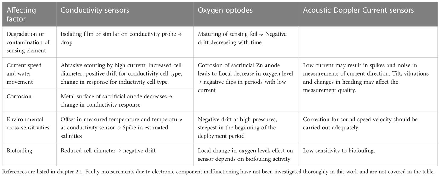
Table 1 Factors commonly affecting conductivity sensors, oxygen optodes and current sensors in long-term operations underwater, and the resulting effect on measurement result.

2.1.1 Degradation or contamination of sensing material

Depending on the measurement technology, sensors may have a sensing material which is exposed directly or indirectly to the harsh conditions in the deep sea.

2.1.1.1 Oxygen optodes

Over long time periods the sensing foil in an oxygen optode may degrade or bleach depending on number of excitations (Tengberg et al., 2006). (Bittig et al., 2018) separate between sensor drift during storage and during deployment. (Bittig et al., 2018) found some indication for an initially stronger, then exponentially decreasing sensitivity, and a positive drift at zero oxygen for oxygen optodes on moored equipment, but note that no sound conclusion could be drawn based on the measured data, and that more studies were recommended.

2.1.1.2 Conductivity sensors

Surface films from oil spills may result in an isolating film of the probe of an electrode type conductivity sensor, causing a sudden drop in measured conductivity.

2.1.2 Current speed

The speed of current where the sensor is deployed may affect the measurement result both directly and indirectly. High currents, especially combined with high concentration of plankton or other substances can result in abrasive scouring, for example of the conductivity cell (Freitag et al., 1999; Ando et al., 2005; Venkatesan et al., 2019). This is however not relevant for deep-ocean environments. As pointed out by (Lo Bue et al., 2011), low current and low dispersion environments are typical for the deep ocean.

2.1.3 Corrosion of the sacrificial anode

A sacrificial anode is used as a protection when there are corrosive metals at the measurement platform.

2.1.3.1 Conductivity sensors

If the sacrificial anode is too close to the sensor element, its metal surface decreases as it corrodes, and this has a direct effect on the local conductivity (Cardin et al., 2017).

2.1.3.2 Oxygen optodes

The chemical reaction consumes oxygen when metal is in contact with anode, resulting in local dips of oxygen concentration (Cardin et al., 2017). In situations with low currents (ref. previous paragraph) these local dips might not dissipate efficiently (Lo Bue et al., 2011), and the oxygen measurements are therefore less representative of the environment the sensor is intended to measure.

2.1.4 Sensor platform movement

If the sensor platform is moved, this may result in change or local spikes in the measurements (for example of oxygen concentration, conductivity, temperature, pressure). If measurement data are used for making statistics or as input to models, this may lead to erroneous results if the effects due to platform movement are not taken into account. For current sensors, one factor that could lower the quality of current measurements is how well the current sensor is able to compensate for tilt, vibrations and changes in heading for the sensor platform (Tracey et al., 2013).

2.1.5 Measurement conditions/environmental cross-sensitivity

A sensor is in most cases not only sensitive to the parameter it is aiming to measure, but will also be affected by other environmental parameters such as pressure or temperature. Additional measurements of affecting parameters are therefore often used to correct the sensor output. This environmental cross-sensitivity should be taken into account when calibrating the sensor prior to deployment, to establish a measurement function enabling continuous correction of such environmental effects. (Berntsson et al., 1997), (Tengberg et al., 2006) recommend that multivariate calibration should be considered for sensor technologies where the measurement result is highly correlated with multiple parameters. The extreme pressure and temperature conditions encountered in the deep ocean may pose challenges related to calibration. At high pressures the temperature may fall below 0°C, and a regular temperature calibration using water is not possible due to freezing. Effects on the sensing elements due to very high pressure can also cause measurement errors.

2.1.5.1 Conductivity sensors

As salinity is estimated as a function of measured conductivity and measured temperature, the quality of the temperature measurement will influence the quality of the estimated salinity. An offset between the temperature in the conductivity cell and the measured temperature at a slightly different location may lead to spikes and thus more noise in the estimated salinities, especially in environments with rapidly changing temperatures (Jansen et al., 2021).

2.1.5.2 Oxygen optodes

(Bittig et al., 2018) give a detailed overview of how environmental factors affect oxygen concentration measurements by optodes, listing both temperature, pressure and salinity as parameters that should be corrected for. An individual (as opposite to batch) multi-point calibration, including a characterization of the temperature dependency is recommended to minimize the effects of the affecting parameters (Bittig et al., 2018). For high pressure environments (depths larger 2000 m), a negative, foil dependent drift has been observed, steepest at the beginning of the deployment period (Koelling et al., 2022).

2.1.6 Biofouling

Biofouling on sensors is mainly the focus for instruments deployed in shallower water exposed to sunlight, and less critical for stationary instruments that are permanently deployed in the deep-sea. However, macrofauna is observed also in deep-sea ecosystems (Kamenev et al., 2022). There are observations of fouling also at instruments long-term deployed in the deep sea, as reported by (Blanco et al., 2013) and evidence that biofouling may grow on plastic pollution sinking and accumulating in the hadal zone over time, described by (Peng et al., 2020). In addition, Autonomous Underwater Vehicles may spend part of their deployed time exposed to biofouling in shallower water. We therefore find it relevant and necessary to include a discussion of potential effects of biofouling on sensor performance, also for deep sea observations. Biofouling can cover the sensing element and thus directly affect measurements, but it can also change the local environment around the sensing element.

2.1.6.1 Conductivity sensors

Biofouling can reduce the cell diameter of the electrode type conductivity cell (Venkatesan et al., 2019), resulting in an apparent increase in resistance and thus a negative drift (Bigorre & Galbraith, 2018), (Alory et al., 2015). Conductivity sensors based on the inductive principle are less sensitive to biofouling than electrode type conductivity cell sensors (Aanderaa Data Instruments AS, 2013), but a decrease in sensor bore diameter due to biofouling may still cause a negative drift (Gilbert et al., 2008), (Aanderaa Data Instruments AS, 2013), (Friedrich et al., 2014), (Tengberg et al., 2013).

2.1.6.2 Oxygen optodes

Oxygen optodes are primarily affected by biofouling indirectly, as the presence of fouling close to the sensing foil alters the oxygen content in the immediate environment. This effect is described in (Tengberg et al., 2006) and (Friedrich et al., 2014).

2.1.7 Electronic component malfunctioning

Errors in the sensor electronics may come from external factors such as vibrations before and during the deployment and ingression of seawater, or from internal factors such as drift in electronic components. One example of this is self-heating of the sensor electronics, which may affect measurements, lead to other electronic component failures and to a premature battery discharge. If water enters into the sensor housing, this may directly affect the sensor element and the sensor electronics, and usually the sensor stops operating. The effect on the measurement may range from sporadic outliers, a decreased signal to noise ratio, a sudden offset, a gradual drift or even a frozen value to complete sensor and communication failure.

2.1.8 Acoustic noise

For instruments sensitive to acoustic noise as well as for acoustic communication of measurement data, it is relevant to mention that (Dziak et al., 2017) measured and evaluated the acoustic noise levels in the Challenger trench, and listed both seismic activity (as earthquakes), biological activity (as whale communication) and anthropogenic activity (as shipping, seismic air guns for oil and gas exploration, active sonars), in addition to storm-induced wind- and wave noise propagating from the surface to the largest depths. Although somewhat sheltered both from the trench walls and refraction in heterogenous water layers, (Dziak et al., 2017) observed that the noise levels in deep waters were still significant in the deep hadal trench.

2.2 System limitations due to subsea application

In this chapter we discuss system limitations for long-term deployed autonomous sensors operating subsea, relying on wireless communication of measurement data.

Sensors on moored observation equipment are today typically calibrated before and after deployment. In situ calibration campaigns can also be carried out, where the equipment is mounted, calibrated on a ship and re-deployed directly. Depending on the sensor technology and reference instrumentation available at the ship, such in situ calibration may consist of multi-point comparison and adjustment, or only of comparing a few measurement values against a reference. Using the vocabulary proposed by (BIPM et al., 2012), a calibration (comparison against a reference) is performed in both cases, but the term in situ (point wise) verification may be a more intuitive term for the latter case without adjustment. The in situ calibration or verification campaigns can be performed on regular time intervals which depend on the expected variability of the measured variable – which may differ significantly between seasons. Sensors on AUVs can be compared with neighbor sensors when two vehicles are sufficiently close, or sensors on (Argo) gliders can autocalibrate when the vehicle surfaces, as an in-air reading by oxygen optodes (Bittig and Körtzinger, 2015; Johnson et al., 2015; Nicholson & Feen, 2017; Bittig et al., 2018). For long-term deployed sensors in the deep sea however, periodic in situ calibration from ships may be practically and economically challenging, due to the remote measurement locations and large depths. This lack of access to external calibration leads to a need for on-line data quality control, self-validation and diagnostics at the sensor level and through the sensor network.

Deep-sea observation equipment relying on underwater wireless communication would need to adapt to severe limitations on data rates and battery capacity. In the case of acoustic communication, the underwater speed of sound is much lower than speed of light, resulting in long propagation delays and high doppler distortion, and only low frequencies are possible for communicating over the long ranges typically encountered in deep sea exploration (Van Walree et al., 2022). Underwater acoustic communication has high power demands, and continuous transmission of sensor raw data will be too energy-demanding, in practice infeasible for deep sea applications. As a natural consequence, more of the signal pre-processing must be handled locally on the sensor prior to transmission. This includes calculation of measurement output signal based on input measurements, averaging, but also filtering out of erroneous data. (Woo & Gao, 2020) point to data processing at sensor level to filter out information that is not relevant to avoid overloading of a network communication channel. Computationally demanding algorithms for real-time processing are however limited by the available battery power (Whitt et al., 2020). Battery lifetime can be optimized by intelligent data transmission strategies and active use of power saving mode combined with adaptive sampling schemes, for example as described by (Law et al., 2009). Depending on the intended use of the data, different time-resolutions may be required for different parameters, and a possibility for the user to adjust sampling rates remotely would be useful.

2.3 Data description

Historical measurement data from moored pressure, conductivity, temperature, and oxygen sensors (SeaGuard, Aanderaa Data Instruments) deployed in deep-ocean environments in the Drake Passage (≈3950 m, data from 2009-2010, 60 minutes measurement interval) and Deep Atlantic (≈4000 m, data from 2010-2011, 20 minutes measurement interval) are used for illustrating the algorithms for sensor self-validation described in chapter 2.4. In the Drake Passage, data from two SeaGuards at different heights were compared, referred to as Drake 136 and Drake 137.

Table 2 give more information on the sensors. The Drake Passage and Deep Atlantic moorings were not part of a wireless network for acoustic communication of measurement data. We use this historical data for illustrating the proposed algorithms for real-time quality control at the sensor node which would be highly beneficial if the data from the moorings were a part of a wireless network. The measurement data is provided as Supplementary Material: Data Sheet 1.CSV for Drake Passage, Data Sheet 2. CSV for Deep Atlantic 136 and Data Sheet 3. CSV for Deep Atlantic 137.

TABLE 2

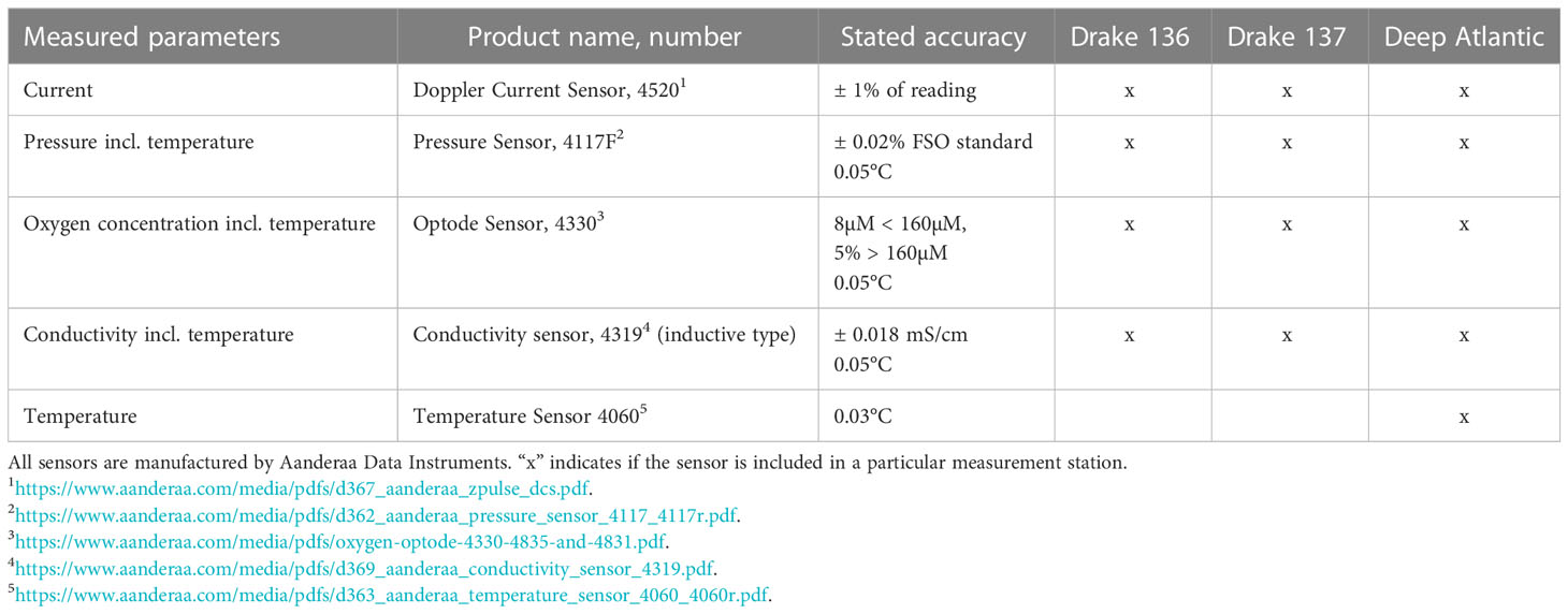
Table 2 Sensor descriptions and stated accuracies.

2.4 Algorithms for sensor self-validation

In this chapter we describe algorithms for sensor self-validation which are tailored for real-time, in situ operation on sensor node level, considering the system limitations and challenges as described in chapter 2.2. We identify and compare quality control manuals currently referred to in the oceanographic measurement community (chapter 2.4.1). We proceeded to investigate methods to extend automated real-time data quality control to cover some of the checks which are now typically performed in delayed mode. Based on proposals found in some of the manuals on quality control for oceanographic measurement data, we propose tests combining measurements of different variables (chapter 2.4.2). To enable detection of sensor element or electronic drift, we also investigate strategies for automatic sensor self-validation relying on redundant measurements (chapter 2.4.3). Test results are presented in chapter 3.

2.4.1 Quality control currently applied in oceanographic measurements

Most of the guidelines and recommendations related to data quality control procedures in the oceanographic community are collected and accessible from the Ocean Best Practice System (OBPS) (Pearlman et al., 2019). In (Bushnell et al., 2019), established quality assurance of oceanographic observations are categorized into real-time, near real-time, delayed mode and reanalysis quality control.

For CTD devices, there are several best practices/recommendations proposed by the various projects or networks operating such equipment. The U.S. Integrated Ocean Observing System (IOOS) proposes a manual for real-time quality control (U.S. Integrated Ocean Observing System, 2020b). In addition to corrections due to response time and thermal mass, the manual lists a set of required tests (gap, syntax, location, gross range, climatological), strongly recommended tests (spike, rate of change and flat line), and suggested tests (multi-variate, attenuated signal, neighbor, Temperature-Salinity (TS) curve/space, density inversion). The QARTOD (Quality Assurance/Quality Control of Real-Time Oceanographic Data) initiative (U.S. Integrated Ocean Observing System, 2020b) stresses among others that observations should have a quality descriptor (for instance quality control flags pass, suspect, fail) and be subject to automated real-time quality test. The Argo Quality Control manual for CTD devices (Wong et al., 2022) describes two levels for quality control and eventual adjustment: A real-time, automatic system and a delayed-mode system requiring expert interference. The Copernicus project for marine environment monitoring has published “Recommendations for in-situ data Near Real Time Quality Control” (EuroGOOS DATA-MEQ Working Group, 2010), listing automatic tests comparable to the ones recommended by the QARTOD and Argo Float programs. The Pan-European Infrastructure for Ocean & Marine Data Management (SeaDataNet) proposes a data Quality Control manual (SeaDataNet, 2010), together with a list of quality flags. In addition to valid date, time, position, global and regional ranges, the SeaDataNet manual proposes checks for instrument comparison.

The International Oceanographic Data and Information Exchange committee (IODE) and the Joint Commission on Oceanography and Marine Meteorology (JCOMM) have through the “Global Temperature and Salinity Profile Programme GTSPP” issued the “GTSPP Real-Time Quality Control Manual” (UNESCO-IOC, 2010). This manual proposes several tests aimed at Temperature and Salinity profiles, but also relevant for other marine data. The tests are grouped into different stages, ranging from position, time, and profile identification checks to consistency with climatologies, and finally to internal consistency checks before a visual inspection. Below is an overview of basic tests proposed by established manuals (EuroGOOS DATA-MEQ Working Group, 2010; U.S. Integrated Ocean Observing System, 2020b; Wong et al., 2022) for (near) real time quality control of oceanographic sensor data, adapted for this work as described by the pseudocode.

● Valid range: If value is outside the given range, then fail.

● Flat line: If n consecutive values differ less than ϵ, then fail.

● Spike – absolute threshold: If the value of a measurement i is more than a sensitivity factor S times the average of measurements i-1 and i+1, then fail.

● Spike – dynamic threshold: If the value of a measurement i is more than a sensitivity factor S times the standard deviation of the n last measurements, then fail.

● Rate of Change – threshold based on first month of data: If ((abs(measurement i – measurement i-1)+abs(measurement i - measurement i+1)) > 2·2·std.dev(first month), then fail.

● Rate of Change – dynamic threshold: If the difference between measurement i and i+1 is more than a threshold S times the standard deviation of the n last measurements, then fail.

The results of the tests are recommended Quality Flags, to be approved by the operator. The “GTSPP Real-Time Quality Control Manual” (UNESCO-IOC, 2010) expects that some of the process of visual inspection can be converted to objective tests but points out that there will always be a need for visual inspection. The manual further proposes that variables may be calculated based on others, to evaluate if the observed values are reasonable (for instance density based on temperature and salinity).

Both (SeaDataNet, 2010) and (U.S. Integrated Ocean Observing System, 2020b) propose some form of multi-variate test to make use of the correlations between related variables, but it is acknowledged that such tests are considered advanced and not usually implemented as a part of (near) real-time quality control. In addition to the (near) real-time quality control tests proposed in the manuals referred to above, extensive guidance for quality control typically performed as delayed mode are provided by (Thomson & Emery, 2014) and (Kelly, 2018).

2.4.2 Test based on correlated parameters

In delayed mode inspection of measurement data by experts, a scatter plot over the whole measurement period of related variables can be very useful for detecting measurement anomalies (Thomson & Emery, 2014). However, this is not adaptable to real-time autonomous sensor self-validation. We therefore propose two other methods for exploiting correlated measurements below.

• Label one variable based on a breached threshold for an affecting variable

One use especially relevant for deep-ocean conditions, is to label oxygen concentration measurements where the current velocity is below a set threshold to indicate possible sacrificial anode oxygen consumption (as discussed in 2.1.3). Another example is where the moorings are dragged down or moved. Such movement can be detected by comparing pressure measurements against a set threshold, and parameters which may be affected by this can be labelled accordingly. In more generic terms, measurements of variable 1 are marked as suspicious (or faulty), if the value or rate of change of a related variable 2 is below or above a certain threshold.

• Running correlation between pairwise related variables

Another possibility is to calculate the running covariance for pairwise related variables. A challenge with this method is to discern between a change in the correlation due to an erroneous measurement, and due to a change in the environmental conditions affecting the two variables differently. Designing a test based on the running correlation will therefore require detailed knowledge of both the sensor technology and the expected environmental conditions and events.

It is important that a basic time-stamp verification test is carried out before different measurements are combined or compared.

2.4.3 Reference measurements

An important limitation to the basic quality checks proposed in existing manuals for (near) real-time quality control is that they cannot be used to detect gradual changes in long-term system response such as sensor drift. To detect a systematic error, either constant or varying with time or other variables, a comparison with an independent estimate of the same variable is required. In this section we list different types of reference measurements that can be used for detecting systematic errors.

2.4.3.1 Internal reference measurements

For many sensor technologies, a point-based local reference measurement can be used to correct a model parameter. A zero-point reference reading gives the system response in absence of any measurement signal or external excitation. In practice such reference measurements are tailored to specific measurement technology. One example is the reference phase reading by use of a red LED that does not produce fluorescence in the foil, implemented in Aanderaa oxygen optodes (Aanderaa Data Instruments AS, 2017). Another example is magnetic or Hall sensors with internal reference measurements using internal chip heaters (Schütze et al., 2018).

2.4.3.2 Redundant measurements at sensor node

Depending on the sensor node configuration, more than one measurement of the same parameter may be carried out sufficiently close, enabling pairwise verification by comparison. In deep sea environments where battery power is a scarce resource, a variation of such a test could be a duty-master configuration, commonly found in metering stations for custody transfer of petroleum liquids (Americal Petroleum Institute, 2016), (Skålvik et al., 2018). A high-quality sensor, possibly with self-validation systems or biofouling protection can be activated at defined intervals, providing reference for validation of a (set of) regular sensor(s). Depending on the measurement principle, the master sensor can be partially protected from environmental wear and tear, thus prolonging the duration of its status as a high-quality reference. It is a clear advantage if different measurement technologies are used to obtain the redundant measurement, reducing the risk of common-mode errors such as uncorrected influencing environmental effects, electronic or sensor element drift, among others.

For mobile sensing units, the “neighbor test” proposed in the Argo manual for CTD Real time QC (Wong et al., 2022) is an example of a redundancy-based test, modified to apply to measurements with a certain distance in both space and time. In the Drake Passage dataset, measurement data from two nodes deployed close to each other provide redundant measurements that can be monitored both by setting absolute difference thresholds and by calculating running correlations between measurements of the same variable. Note that the definition of “acceptable close” depends on the variability of the environment, as well as the targeted data quality in terms of uncertainty.

2.4.3.3 Analytic redundancy/modelling surrogates

If the measured quantity can be estimated from combining measurements of other parameters, this estimate can be used as an analytical redundancy or indirect reference measurement. One example of this is the use of modeling surrogates presented by (Jesus et al., 2017), corresponding to “model-based” method for fault detection described in (Li et al., 2020) and (Gao et al., 2015). (Mitchell, 2007) and (Zhu et al., 2021) propose “multi-sensor fusion” to predict a sensor output and compare with the measured values.

Another example for validation of in situ measurements based on redundant measurements and functional relationships, is described in both (Cullison Gray et al., 2011) and (Shangguan et al., 2022). They showed that the relationship between pH and other carbon measurements could be used for data quality control. Once again, a thorough knowledge of the sensor technologies and environmental dynamics is required for exploiting such analytical redundancies. One challenge with this approach is to consider the different time-delays between a change in the environment and change in sensor signal, as well as the distance between the involved sensors, referred to as sampling differences by (Cullison Gray et al., 2011).

3 Results – automatic tests for sensor self-validation

In this chapter we start by presenting the studied data sets from Deep Atlantic and Drake Passage, pointing out errors, outliers and other anomalies which are identified as erroneous or suspicious by manual inspection. We proceed to apply the automatic quality tests recommended by established manuals as listed in chapter 2.4.1, such as flat line/frozen values, spike/outlier, and rate of change, leaving out the most basic range tests. We then show how tests relying on correlations between different parameters as proposed in chapter 2.4.2 can be carried out to identify possible measurement errors related to low current speed and changes in mooring location from pressure measurements, before we move on to a comparison with redundant measurements on the same node and across nodes as proposed in chapter 2.4.3.

3.1 Visual test performed manually as a delayed mode quality control

Although there exist various software packages that can be used to assist in the delayed mode quality control, one important step is the visual identification of suspicious or clearly erroneous data. Figures 1, 2 give an overview of the Deep Atlantic and Drake Passage measurements. Table 3 summarizes the manual quality control observations of the time series. Each distinct observation of any suspicious or erroneous measurement is marked with a unique number (Obs₁, Obs₂, Obs₃ etc.), to enable tracing the observations across the different manual and automatic tests.

FIGURE 1

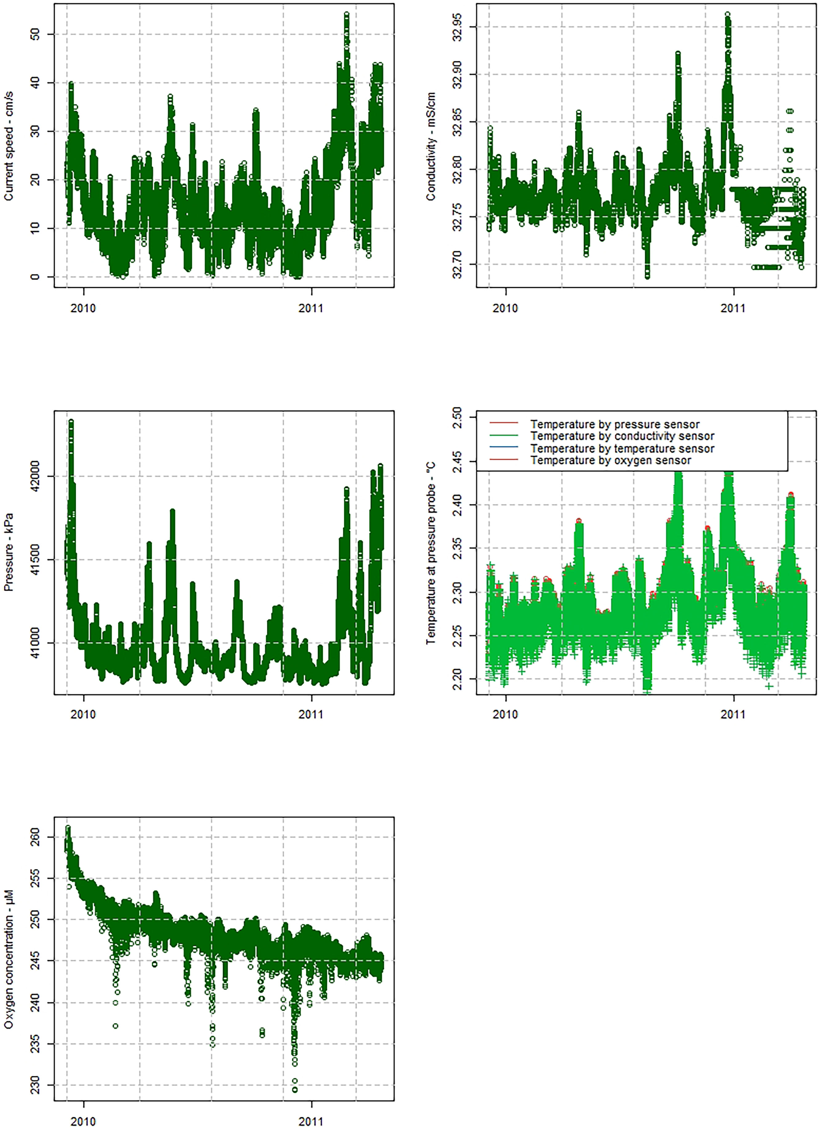
Figure 1 Overview of the Deep Atlantic measurements.

FIGURE 2

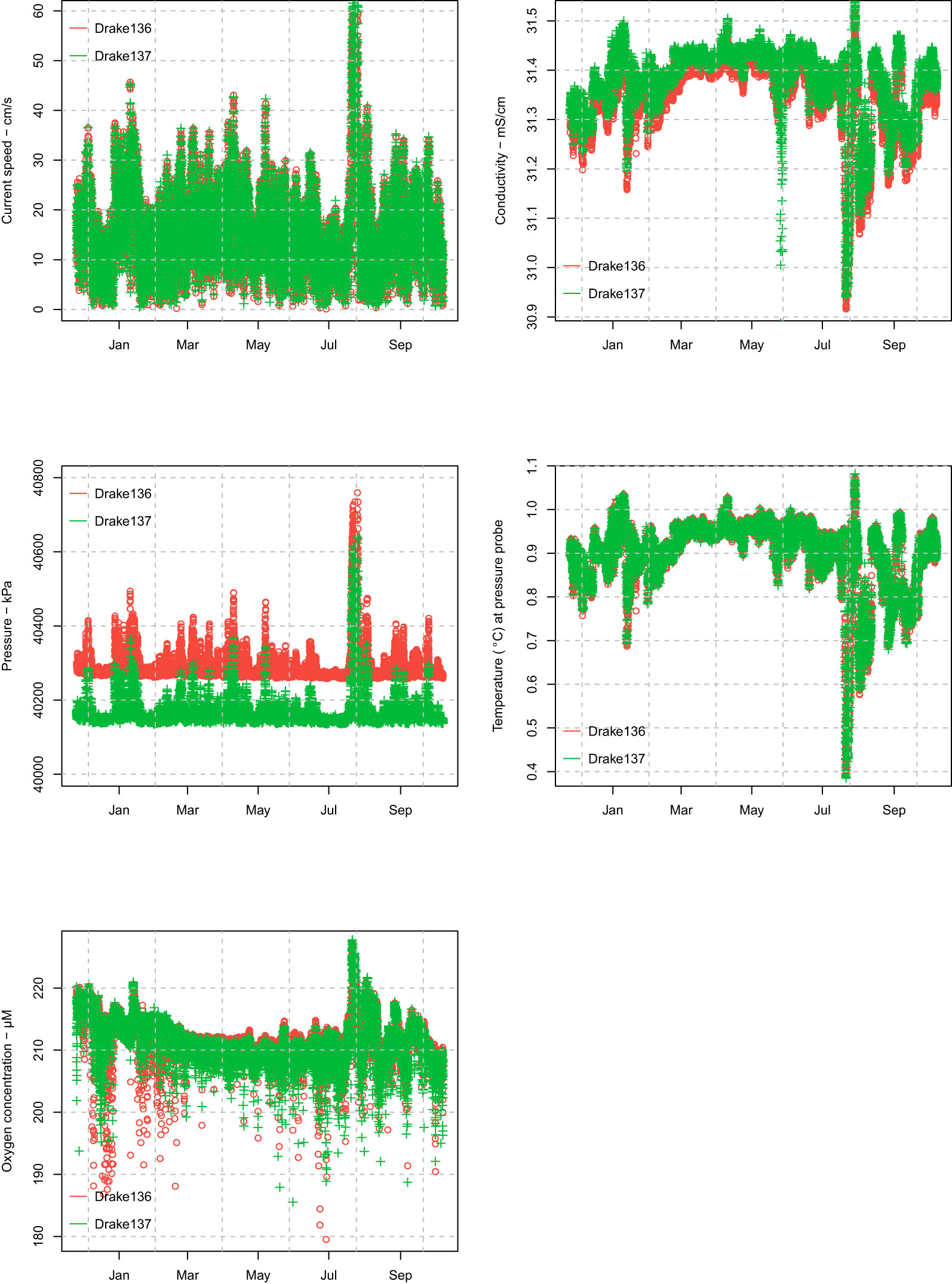
Figure 2 Overview of the Drake 136 and Drake 137 measurements.

TABLE 3

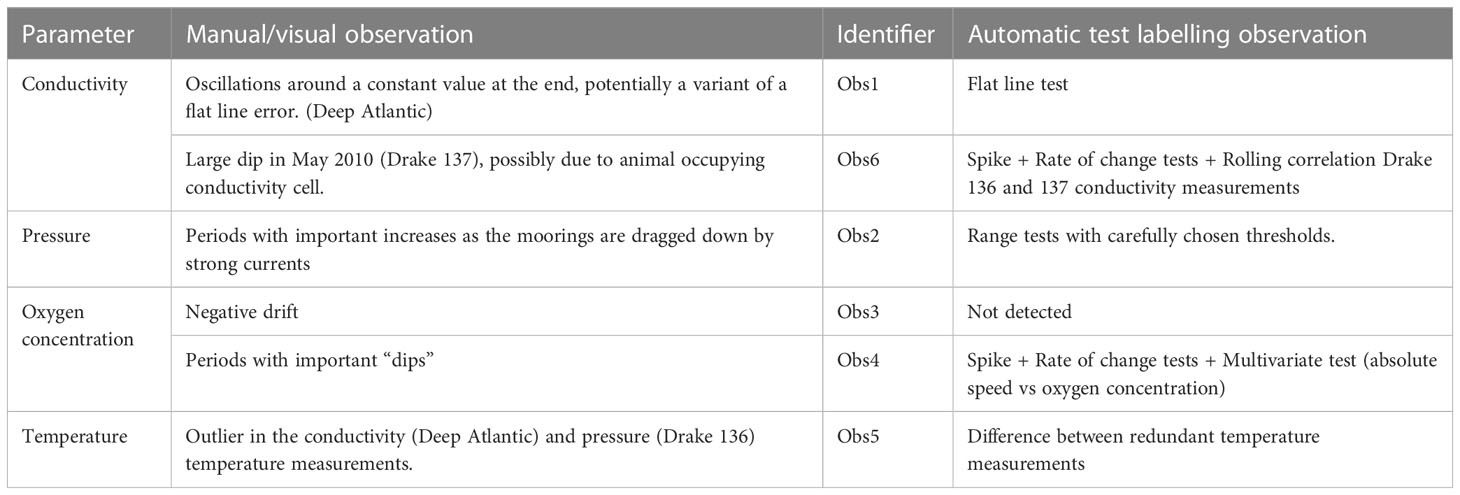
Table 3 Summary of manual observations and automatic tests for labeling data.

3.2 Basic automatic quality tests

Figure 3 shows that the basic flat line test successfully identifies many, but not all, of the Drake Passage conductivity measurements that would be labelled as suspicious or stuck by a visual inspection (Obs1).

FIGURE 3

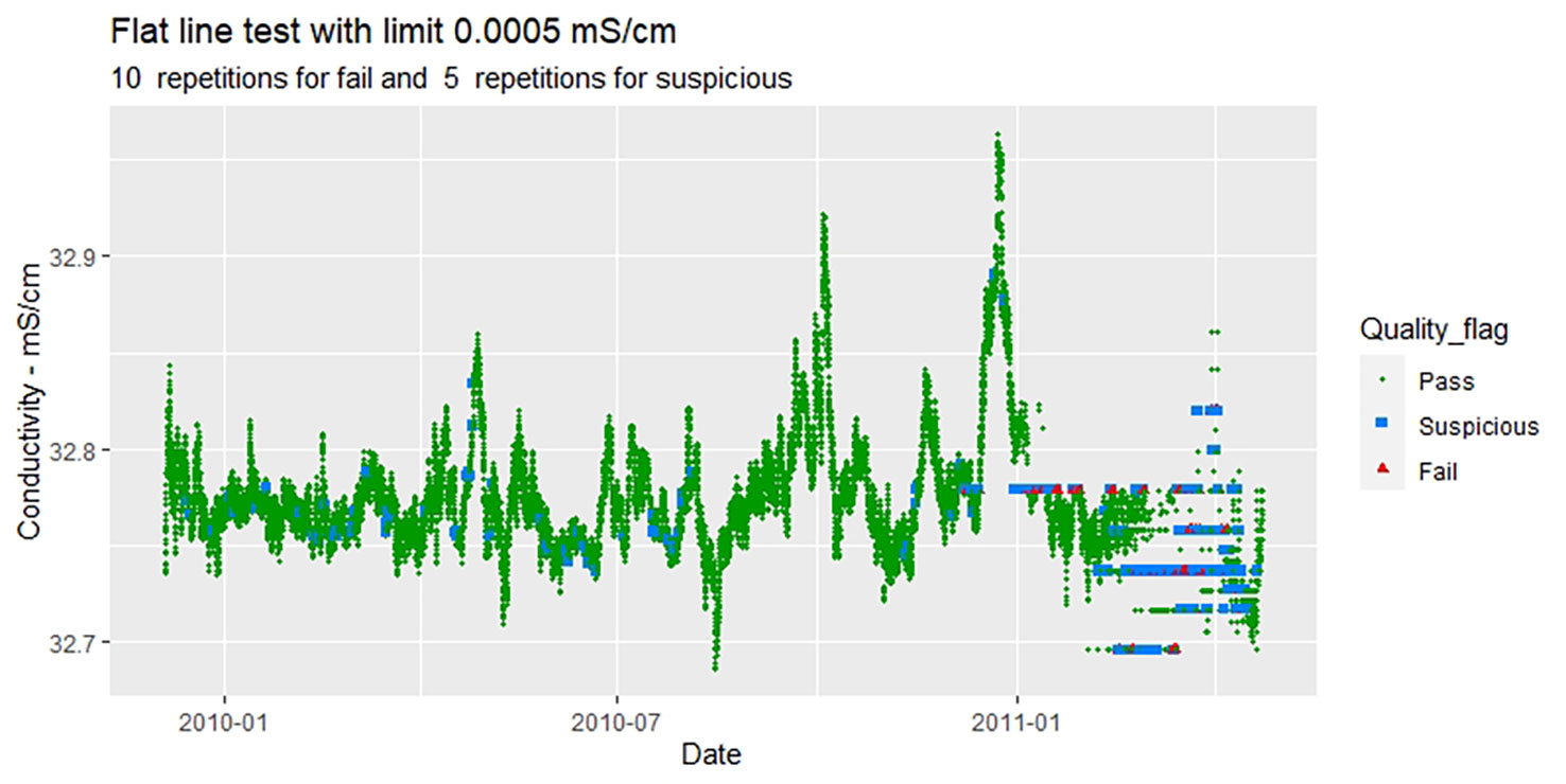
Figure 3 Result of flat line test on Deep Atlantic conductivity measurements. The tests identify many, but not all, of the Drake Passage conductivity measurements that would be labelled as suspicious or stuck by a visual inspection (Obs1).

Both the spike tests and rate of change tests, illustrated in Figure 4 for Drake 136 oxygen concentration, label the spikes in the oxygen concentration measurement as suspicious or erroneous. This corresponds to the manual/visual observation Obs4. We notice from the figures that the test performances strongly depend on the set thresholds and number of measurements used for calculating thresholds based on standard deviation (further discussed in in chapter 4.2). A combination of such tests could result in a more robust performance, (further discussed in in chapter 4.3). Similarly, Figure 5 shows that the automatic tests detect a strong dip in Drake137 conductivity measurements in June 2010, corresponding to the manual/visual observation Obs6. The best performing test was a rate of change test with threshold set from the standard deviation in the first month as proposed by (EuroGOOS DATA-MEQ Working Group, 2010).

FIGURE 4

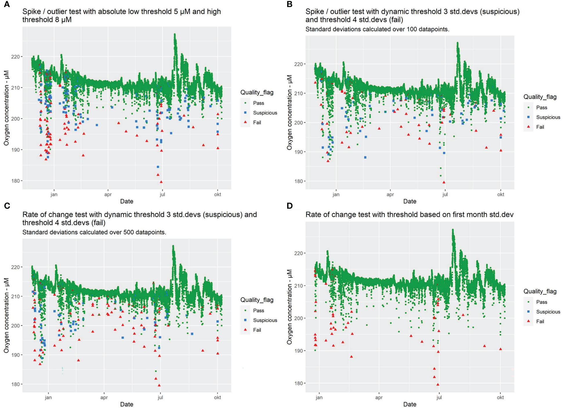
Figure 4 Spike/outlier and rate of change tests, for oxygen concentrations measured at the Drake 136 node. (A) shows a spike/outlier test with absolute thresholds 5 μM and 8 μM for suspicious and fail labels respectively. (B) shows a spike/outlier test with dynamic thresholds set as 3 times and 4 times the standard deviation of the last 100 measurements for suspicious and fail labels respectively. (C) shows a rate of change test with dynamic thresholds set as 3 times and 4 times the standard deviation of the last 500 measurements for suspicious and fail labels respectively. (D) shows a rate of change test with a threshold based on the standard deviation of measurements in the first month. The tests identify many, but not all, of the measurements that would be labelled as suspicious or stuck by a visual inspection (Obs4). Similar effects are observed for Drake 137.

FIGURE 5

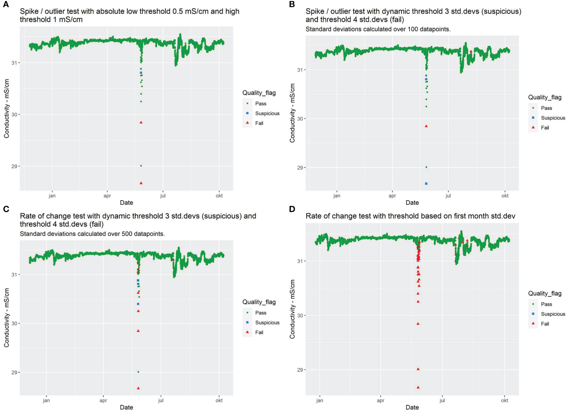
Figure 5 Spike/outlier and rate of change tests, for conductivity measured at the Drake 137 node. (A) shows a spike/outlier test with absolute thresholds 0.5 mS/cm and 1 mS/cm for suspicious and fail labels respectively. (B) shows a spike/outlier test with dynamic thresholds set as 3 times and 4 times the standard deviation of the last 100 measurements for suspicious and fail labels respectively. (C) shows a rate of change test with dynamic thresholds set as 3 times and 4 times the standard deviation of the last 500 measurements for suspicious and fail labels respectively. (D) shows a rate of change test with a threshold based on the standard deviation of measurements in the first month. The dip of approximately 2.5 mS/cm in June 2010 (Obs6) is partially detected by the spike/outlier (A, B) and rate of change test with dynamic threshold (C), and fully detected by the rate of change test based on the standard deviation of the first month of measurements (D).

3.3 Tests based on correlated parameters

Figure 6 shows Drake 136 measurements labelled for low absolute current speeds measured at the same node. The figure shows that a threshold on low currents can be used as a filter for identifying suspicious measurements of oxygen concentrations, and that most (but not all) of the manually observed “dips” in measured oxygen (Obs4) are identified by this test.

FIGURE 6

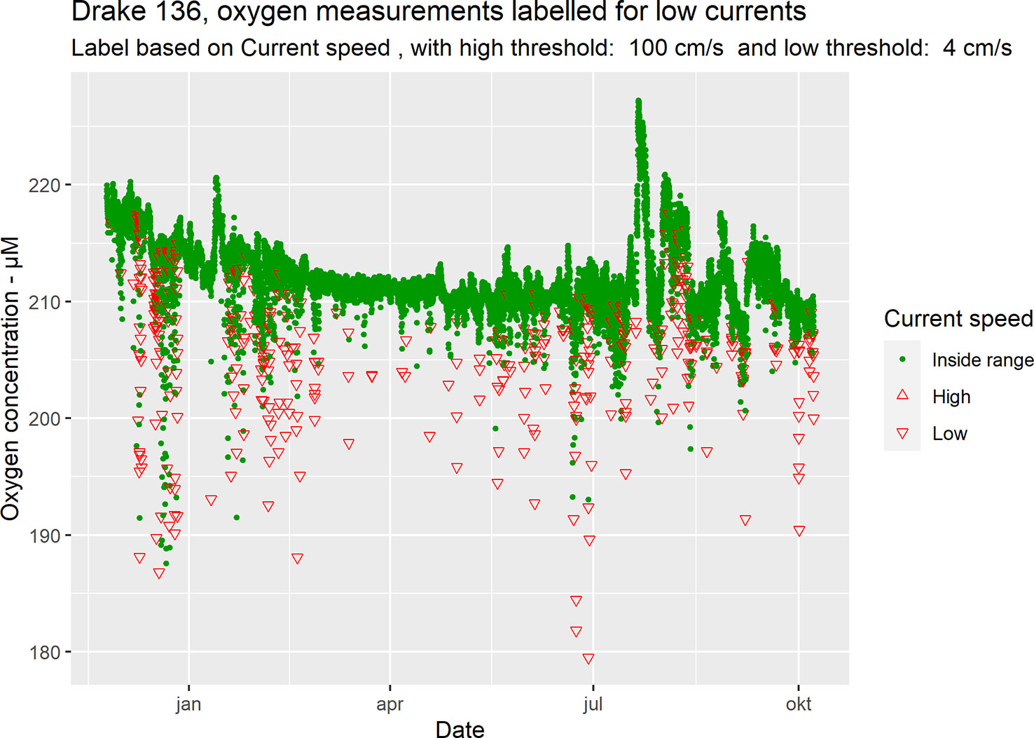
Figure 6 Drake Passage 136, measured oxygen concentration, labelled based on absolute current speed ranges. Most of the manually observed “dips” in measured oxygen (Obs4) coincide with periods with low current speeds. Similar effects are observed for Drake 137.

Figure 7 show Drake 136 measurements labelled for high pressure ranges (Obs2). The test shows that several periods with changes in measured conductivity, increases in measured oxygen concentration as well as changes in temperature measurements are coinciding with increased pressure events. Such observations are not evident from a purely visual delayed mode control. Figure 7 also shows that all periods with measured absolute current speed above ≈35 cm/s are coinciding with increased pressure/depth. Even though these measurements are not necessarily faulty, they are not representative for the intended environment/depth/location, and the labelling is thus useful for filtering data prior to analysis.

FIGURE 7

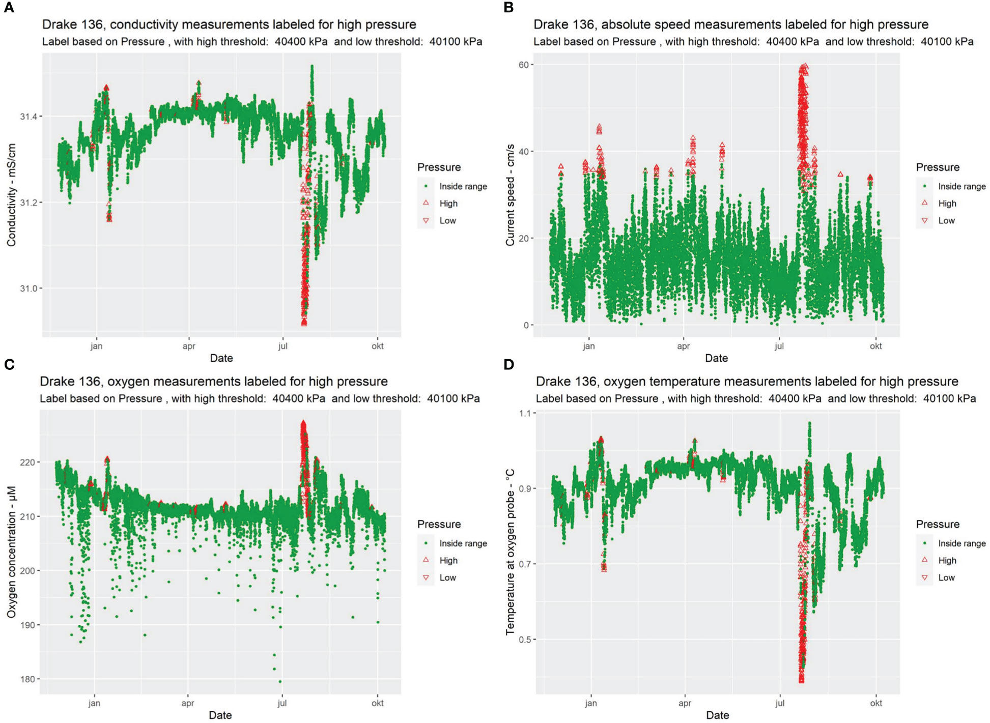
Figure 7 Drake Passage 136 measurements of conductivity (A), current speed (B), oxygen concentration (C) and temperature measurements at the oxygen optode (D), labelled based on pressure ranges (Obs2). A high-pressure threshold is set to 40 400 kPa and a low-pressure threshold is set to 40 100 kPa. Similar effects are observed for Drake 137.

3.4 Redundant measurements of the same parameter

One example of verification by pairwise comparison on a typical CTD-node may be temperature measurements performed by both the conductivity sensor, pressure sensor, and on a dedicated temperature sensor. A change in the deviation between temperature measurements on the same node may be identified automatically on the node level, either by setting a threshold on the absolute difference or on the running correlation between the measurements.

Figure 8 shows that the difference between the Deep Atlantic conductivity temperature measurement and temperature measurements are above the set threshold for one specific data point in April 2011, which corresponds to the manual/visual Obs5. Figure 9 shows how a test based on the difference between Drake 136 and Drake 137 conductivity measurements can identify the Drake 137 dip in conductivity (Obs6). Similarly, Figure 10 shows how a test based on the difference between Drake 136 and Drake 137 measurements of oxygen concentration identifies many of the manually observed “dips” (Obs4). Figure 11 shows a plot of the difference between Drake 136 and Drake 137 oxygen measurements, labelled for low currents measured at Drake 136, showing that the periods with large differences between the two nodes often correspond to periods with low current speeds. The comparison of two measurements based on the same sensor technology does however not detect the manually observed drift in both Drake 136 and Drake 137 oxygen measurements (Obs3).

FIGURE 8

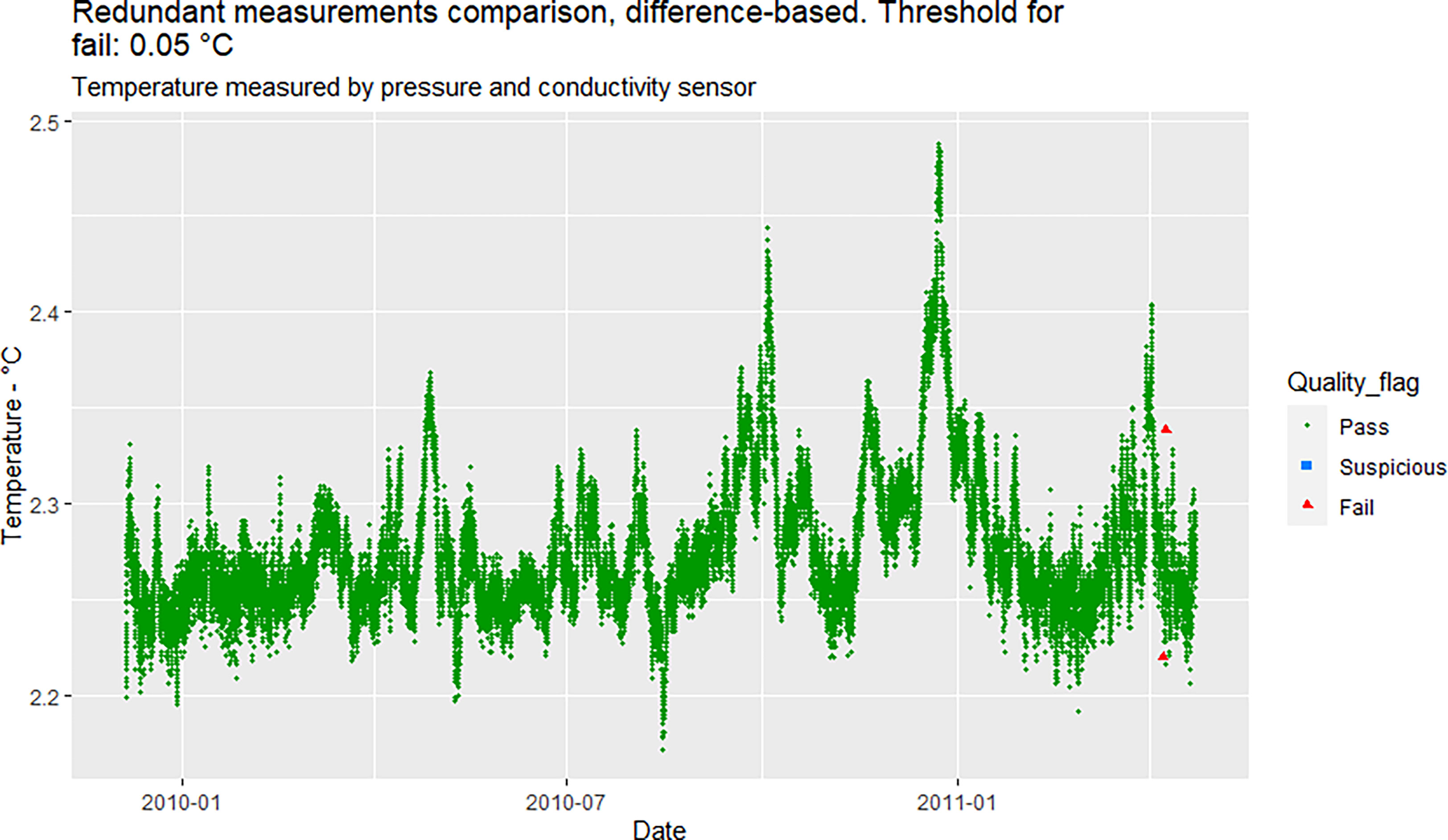
Figure 8 Deep Atlantic temperature measurements, labelled based on differences between temperature measurements at the pressure and conductivity sensor, with a threshold for “Fail” at 0.05°C. The outlier in the conductivity temperature measurement which can be manually observed from a scatterplot in delayed mode (Obs5) is identified by this test.

FIGURE 9

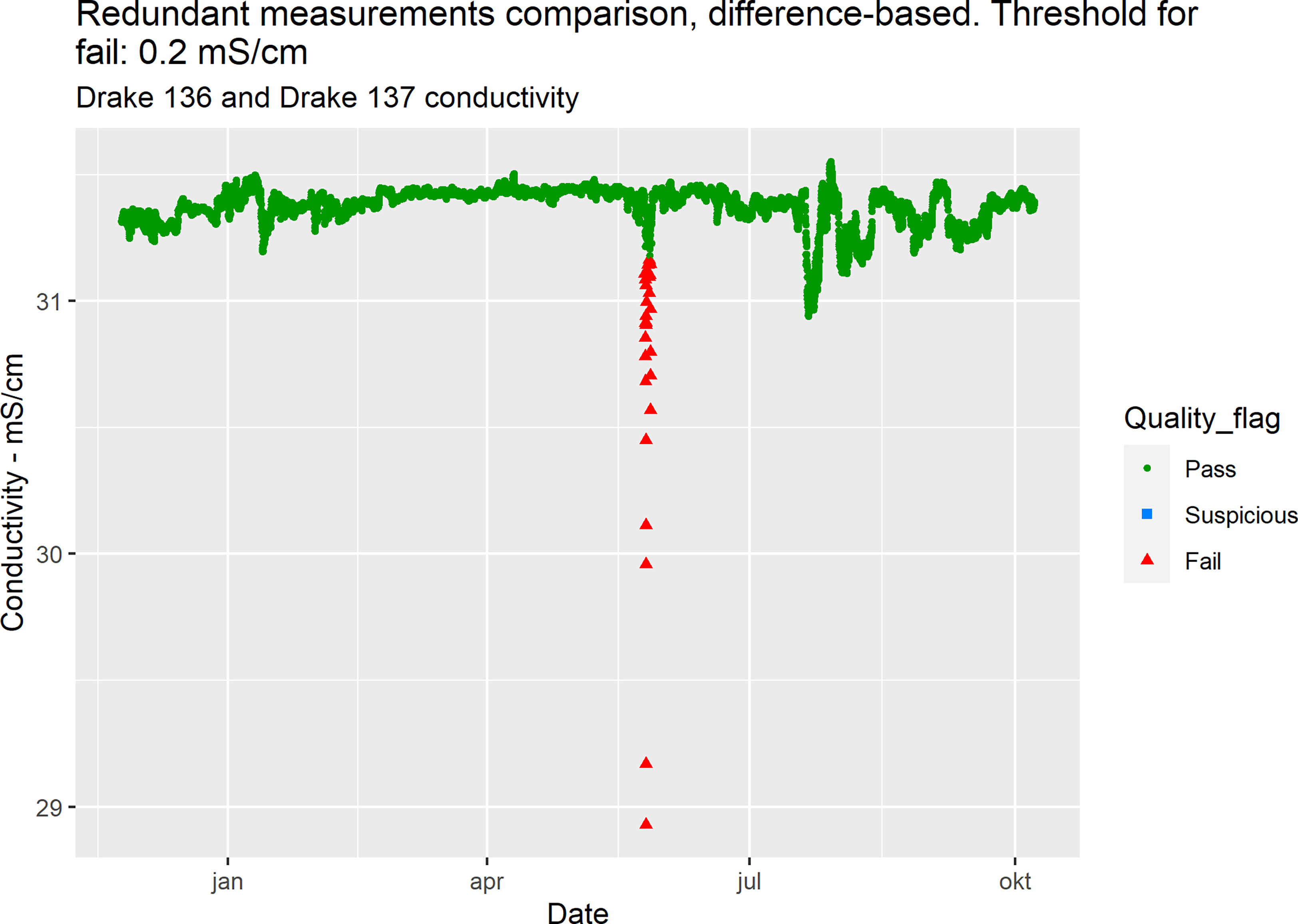
Figure 9 Drake 137 conductivity measurements, labelled based on differences between redundant Drake 136 and Drake 137 measurements, with a threshold of 0.2 mS/cm. The dip of approximately 2.5 mS/cm in June 2010 (Obs6) is labelled as “Fail” by this test.

FIGURE 10

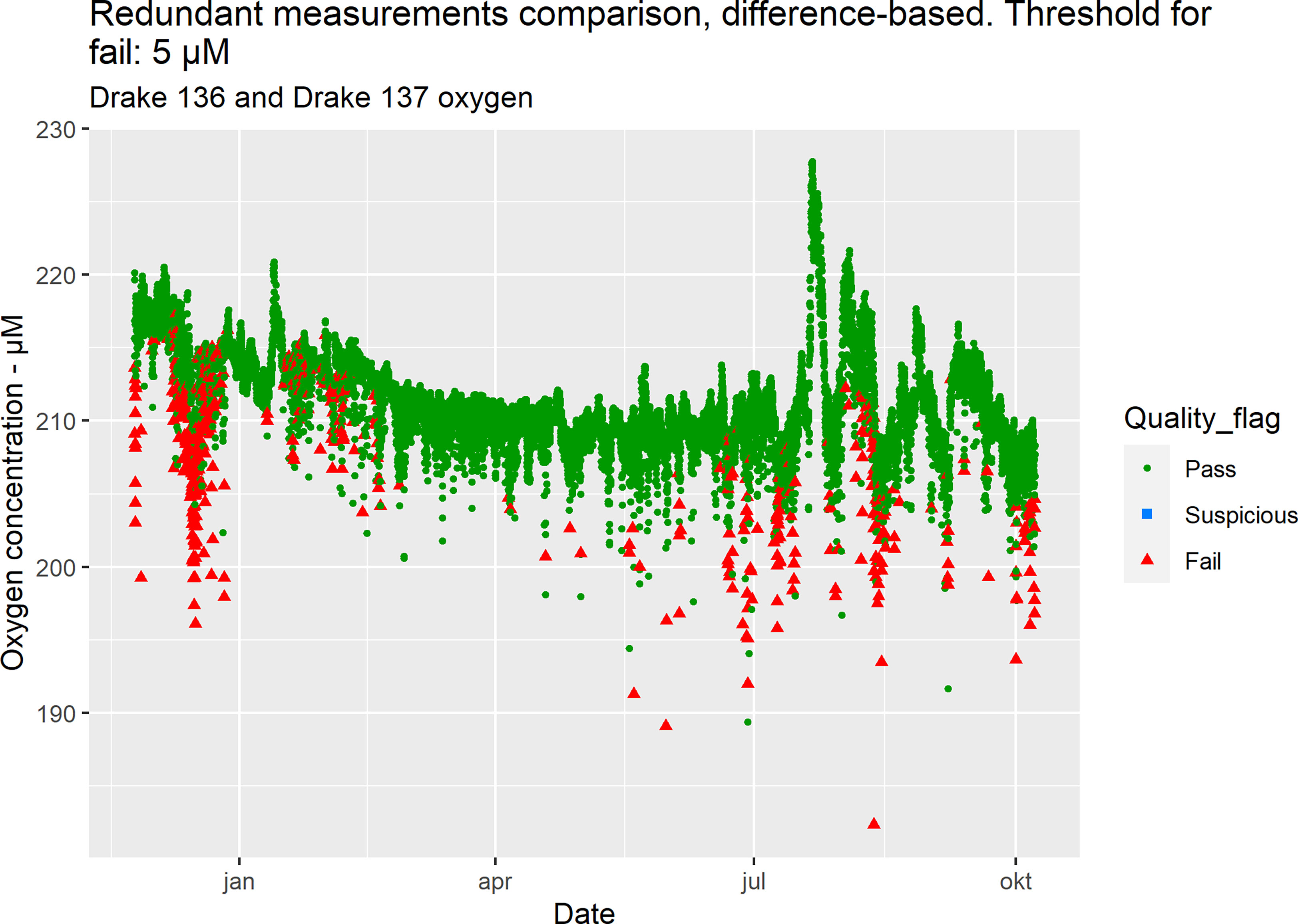
Figure 10 Drake 137 oxygen concentration measurements, labelled based on differences between redundant Drake 136 and Drake 137 measurements, with a threshold of 5 μM. Many of the manually observed “dips” in measured oxygen (Obs4) also result in a difference between the redundant measurements above the set threshold. Similar effects are observed for Drake 137.

FIGURE 11

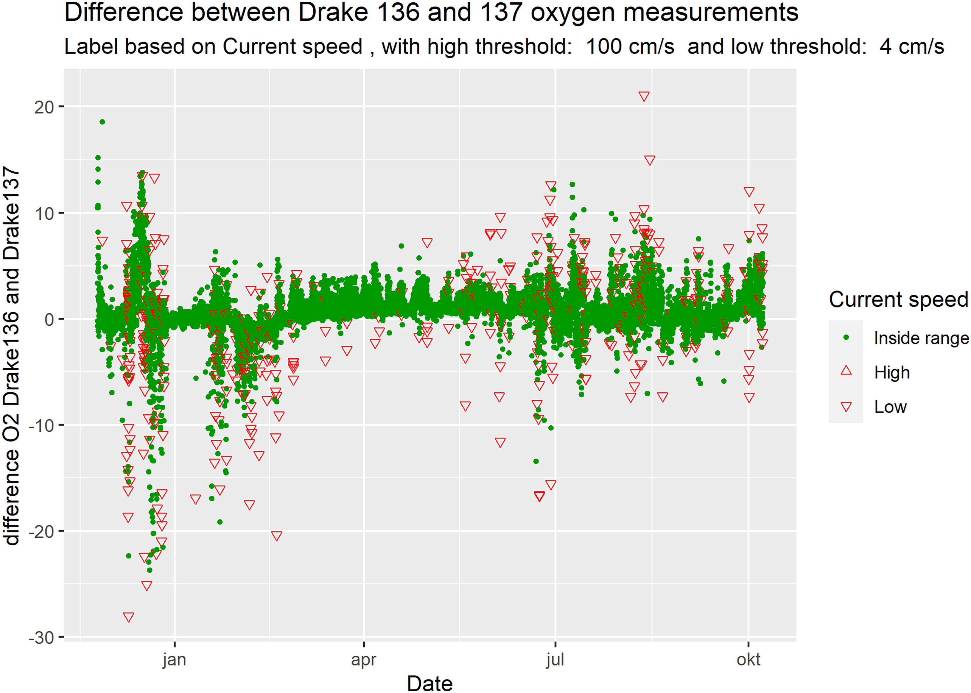
Figure 11 Difference between Drake 136 and Drake 137 oxygen measurements, labelled based on current speed.

Figure 12 shows the running correlation between pairwise conductivity measurements at the Drake 136 and 137 nodes. The running correlation test identifies a strong dip in correlation between the two datasets in the end of May 2010, corresponding to (Obs6).

FIGURE 12

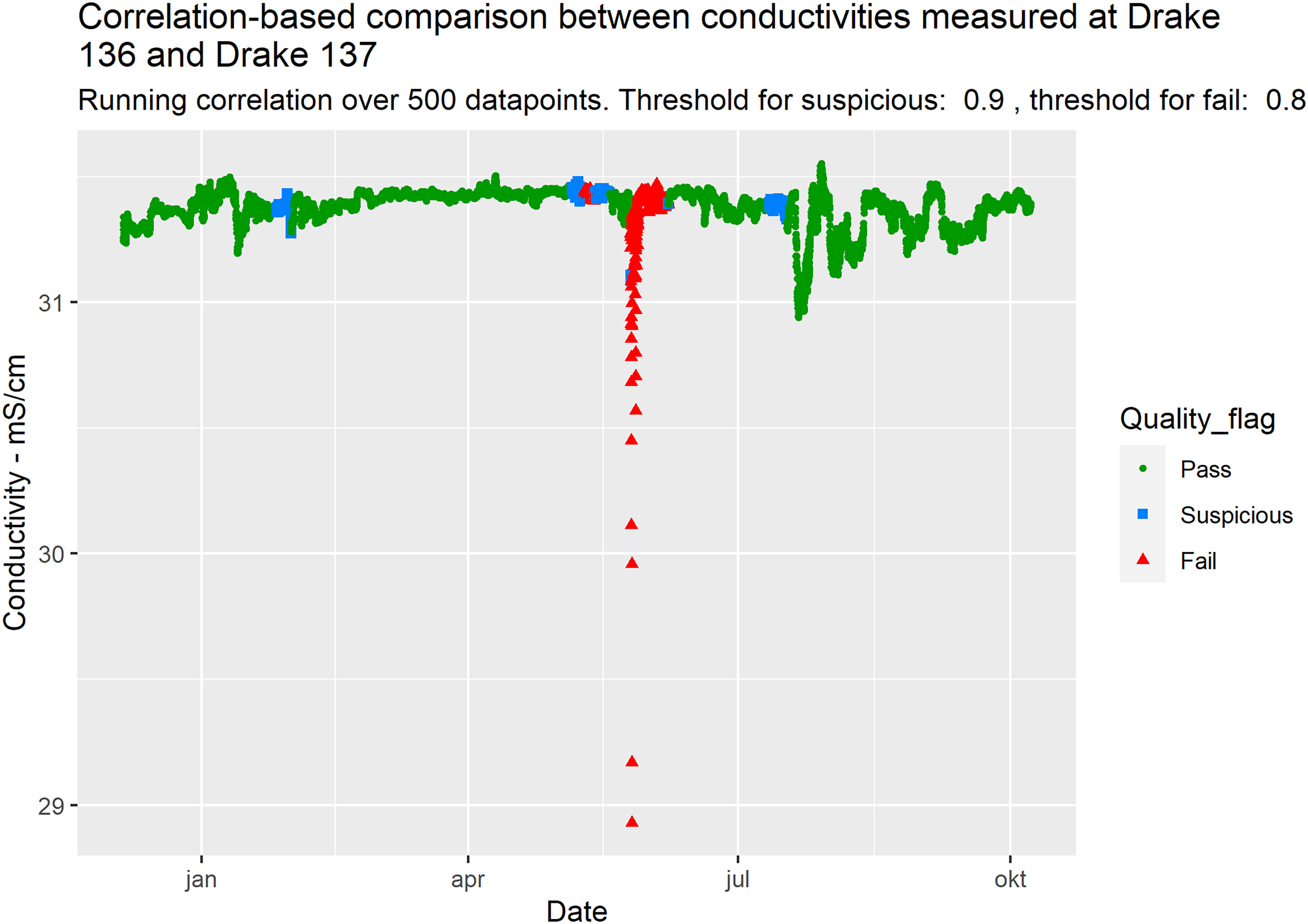
Figure 12 Drake 137 conductivity measurements, labeled based on running correlation (Pearson) over 500 measurements between redundant Drake 136 and Drake 137 measurements, with a threshold of 0.8. The dip of approximately 2.5 mS/cm in June 2010 (Obs6) is labelled as “Fail” by this test.

4 Discussion

We will first evaluate how effective the automatic, real-time tests described in 2.4 are for detecting the manual delayed-mode observations. Then we discuss how knowledge of sensor technology and deep-sea environments are important prerequisites for designing tests and setting well-founded thresholds. We proceed to discuss how tests can be combined to allow for robust sensor self-validation. Furthermore, we argue that limitations imposed by deep sea measurement systems must be balanced against user requirements related to sampling frequency, data availability and quality of measurement. We round off the discussion by highlighting how the choice of sensor quality, calibration frequency, sensor redundance and communication requirements are case specific, before pointing to other data analysis techniques that can be included in tests for sensor self-validation.

4.1 Comparison of manual and automatic observations

Except for the observed drift of the measured oxygen concentration (Obs3), the manual/visual observations of possible measurement errors in the two studied datasets are found to be detectable using automatic tests as long as thresholds and running evaluation time period are set carefully.

For the Deep Atlantic dataset, the oxygen concentration did not correlate strongly enough with any of the other measured variables at the same node to determine if the measurand changes over time or if the manually observed negative drift (Obs3) was related to the sensing element or electronics. Similarly, comparison of the oxygen concentration measurements in the Drake 136 and Drake 137 datasets did not reveal any systematic offset increasing with time. Without information from post-deployment calibration, and only based on the in situ measurements, it is not possible to evaluate if both sensors had approximately equal drift, or if the measured, slow decrease in oxygen concentration was the true evolution of this parameter. A calibration of the sensor upon retrieval can be used for correcting the measurement drift (Koelling et al., 2022), but to detect and correct for drift automatically, real-time and in situ, a redundant measurement relying on a different technology is required.

4.2 Knowledge of sensor technology and the deep-sea environment – setting the right thresholds

The most basic tests proposed in guidance documents and manuals for (near) real-time quality control of oceanographic measurements consist of checking if the measurement is inside the expected range, based on location-specific statistics such as maximum and minimum values, or more general limits based on physical possible values. The other tests proposed by the established oceanographic manuals such as spike, rate of change and flat line tests, rely on setting well-adapted thresholds or sensitivity limits, based on a minimum of sensor technology and environmental knowledge.

For a flat line test, the expected temporal variation of the measurand needs to be considered, as well as sensor sensitivity. For spikes/outlier-detection, and rate of change tests on the other hand, the choice of thresholds is less straight-forward and must be customized for the specific technology and application. Compared with absolute thresholds, dynamic thresholds may be an improvement, but one still must choose a sensitivity level of the detection algorithms. Too sensitive algorithms will result in alarm noise, and too lenient algorithms will detect fewer of the measurement errors.

If the standard deviation of a representative time period is chosen as a basis for the dynamic thresholds, such a period should ideally be identified automatically for sensors to be truly autonomous. The number of measurements to include when calculating such statistics must also be chosen with care.

4.2.1 Environmental dynamics

When setting up tests, a thorough knowledge of both the measurement technology and the expected environmental dynamics (both physical and bio/geochemical) is a pre-requisite. Both spikes/outliers and long-term drift in the measurement signal can be representative of the measurand and should not uncritically be marked as suspicious or erroneous, as illustrated by (Thomson & Emery, 2014). The time-response of the sensor must be seen in relation to the expected time-variability of the measurand/the environmental dynamics.

4.2.2 Measurement uncertainty

To avoid too many false negatives (correct measurements labelled suspicious or erroneous), the intrinsic measurement uncertainty of the sensor should be considered when designing tests. The sensor repeatability, the underlying model uncertainty, the uncertainty in the calibration process; all these uncertainty contributions can be combined to calculate the combined uncertainty of a measurement. A method for estimating the combined uncertainties in measurement systems is detailled in (BIPM, 2008), and a very simplified application of this method to in situ temperature measurements is proposed by (Waldmann et al., 2022).

4.2.3 Intended use

Accurate or precise data, or high (enough) measurement quality are ambiguous terms which may have very different meanings for different applications and different users. One example is how the effect of nearby animals can be perceived as unwanted spikes or measurement noise for one user/application, masking the primary measurand that user intended to measure. For other users primarily interested in biological activity at the measurement site, such spikes can provide valuable information. When data are labelled according to well documented tests, and not deleted, it is easier for new users to re-evaluate the data with a different application in mind. The intended use of the measured data will also play a role when choosing optimal thresholds (Jansen et al., 2021).

4.3 Combining tests

Each automatic test identified some, but not all, of the measurements which visually appear suspicious for a delayed mode inspector. A more robust approach could be to run each test individually on the data set, and then follow some logical rules for combining the different data labels. A multistep solution could also be explored.

4.4 Finding the right balance

The quality control checks recommended in established best practice and guidance documents are typically carried out after data transmission but should in theory be possible to implement locally on the observation equipment. When developing or adapting algorithms for in situ self-validation and self-diagnostic, one must consider deep sea constraints such as communication bandwidth, data processing and power supply limitations. The optimal balance between processing power for in situ quality assurance, battery usage for communication of processed results or data harvesting using AUVs will be very case-specific, but in general there are strong restrictions on power usage, and methods should be chosen with care.

Some of the factors to consider when choosing an optimal self-validation strategy:

● User requirement on data quality and communication

• Measurement resolution

•Transmission frequency

• Measurement uncertainty

• Tolerance against false positives or false negatives

● Sensor coverage/density

● Expected (spatial) variation of the parameter one intends to measure

● Energy consumption of internal signal analysis/treatment of raw data

● Energy consumption of communicating with neighboring sensor

● Sensor cost

● Sensor node battery capacity, CPU performance, memory

4.5 Possible other tests and methods for automatic in situ quality control

4.5.1 Multivariate analysis

An extension of the tests proposed in chapter 2.4.2 is to compare the measurement of more than two parameters and thus take advantage of correlation over multiple dimensions.

4.5.2 Advanced signal analysis

The algorithms explored in this paper are examples of time-domain signal-based analysis. (Gao et al., 2015) divides signal-based fault diagnostic methods into time, frequency, and time-frequency domain. A discrete Fourier transform, among others, can be used to transform data from the time to the frequency domain. Different methods for spectral analysis can then be applied, for instance calculation of the spectral density and periodograms. (Lo Bue et al., 2011) employed a spectral analysis to find that observed drops in measured oxygen were not due to random noise, but had a periodicity related to tidal effects. For systems where the frequency spectrum varies over time, time-frequency analysis methods can be applied for fault diagnostics (Gao et al., 2015).

4.5.3 Neural networks and machine learning

Machine learning can be used for quality control of ocean data (Mieruch et al., 2021), and can be one solution to the challenge of setting efficient thresholds. Based on a separate training dataset or a running training period, the machine learning model will predict a (range of) measurement values. If the discrepancy between the predicted and measured data is higher than a dynamically adopting threshold (see for instance (Blank et al., 2011)), the data will be labeled accordingly. A self-learning method for fault-detection is described in (Li et al., 2020), where fuzzy logic and historical data can be used, provided that the modeler has knowledge of the system. A more data-driven approach also described in (Li et al., 2020) is pattern recognition. (Zhu et al., 2021) separate between self-detection of faults, proposing Least Square Support Vector Machine and back propagation neural network, self-identification of faults from historical data using wavelet packet decomposition for feature extraction, then decision tree algorithms and back propagation neural networks for pattern recognition and classification. (Han et al., 2020) proposes discrete wavelet transforms and grey models for detecting sensor drift, but do not propose any method for discerning between a trend in the measurand itself or an instrument drift. Other methods have been proposed, for example Bayesian calibration of sensor systems (Tancev & Toro, 2022).

As the built-in data processing capacities of existing smart sensors may in many cases not be sufficient to support artificial intelligence algorithms such as machine learning, a dedicated microcomputer installed locally on the sensor node could be an option.

4.5.4 Calibration through network

When several sensors or sensor nodes are operating over a defined geographic location, wirelessly connected through a (acoustic) network, it is possible to calibrate the sensors by comparison with neighboring nodes. (Delaine et al., 2019) separate between reference based and blind pairwise calibration, and (Chen et al., 2016) shows how Data Validation and Reconciliation can be used for calibration through networks.

5 Summary

Deep sea exploration and monitoring requires high-quality measurement data from sensors deployed in harsh conditions. Understanding of how sensors may be affected by the specific environment, combined with knowledge regarding both the parameter and correlations between different variables, are pre-requisites for setting up automatic tests for in situ data quality control. In this paper we have explored, basic range, flat line, spike/outlier, and rate of change tests as proposed in oceanographic real-time quality control manuals, in addition to more complex tests exploiting correlations between different parameters measured on the same or neighboring node. Comparisons between redundant measurements of the same parameter is particularly useful, preferably between sensors based on different measurement principles if the goal is to detect systematic drift.

Machine learning is a promising tool for automatic quality control of measurement data, but simpler, more transparent algorithms are worth investigating further. This is both due to the explainability and traceability of simpler algorithms, but also due to computing, power, and memory limitations for long time deployed sensors in remote locations. As different tests may reveal different types of errors, logic for combining the labels from a set of tests based on detailed knowledge of the measurement system and environment, may enhance the sensors self-validating and self-diagnosing properties. This is subject for future work, together with further exploration of tests in the frequency spectrum and time-series decomposition.

In the broader picture, transparent algorithms with well-documented thresholds for in situ quality control can contribute to increase the trustworthiness and decrease the uncertainty of EOVs (essential ocean variables).

Data availability statement

The original contributions presented in the study are included in the article/Supplementary Material. Further inquiries can be directed to the corresponding author.

Author contributions

AS, CS and K-EF have contributed to the conception of the work. AT has provided the data. AS, CS and AT have performed data analysis and interpretation. AS has drafted the article. All authors (AS, CS, K-EF, AT, and RB) have contributed to critically reviewing and commenting on the draft. All authors contributed to the article and approved the submitted version.

Funding

This work is part of the SFI Smart Ocean (a Centre for Research-based Innovation). The Centre is funded by the partners in the Centre and the Research Council of Norway (project no. 309612).

Acknowledgments

The authors would like to thank Aanderaa Data Instruments AS for providing the data sets, and the two reviewers of Frontiers in Marine Science for the time they invested in carefully reading the manuscript, and for their valuable comments that improved the quality of the paper.

Conflict of interest

AT is employed at Aanderaa Data Instruments AS, a Xylem brand, producing the sensors used in this study.

The remaining authors declare that the research was conducted in the absence of any commercial or financial relationships that could be construed as a potential conflict of interest.

Publisher’s note

All claims expressed in this article are solely those of the authors and do not necessarily represent those of their affiliated organizations, or those of the publisher, the editors and the reviewers. Any product that may be evaluated in this article, or claim that may be made by its manufacturer, is not guaranteed or endorsed by the publisher.

Supplementary material

The Supplementary Material for this article can be found online at: https://www.frontiersin.org/articles/10.3389/fmars.2023.1152236/full#supplementary-material

Footnotes

1. ^ https://www.aanderaa.com/media/pdfs/d367_aanderaa_zpulse_dcs.pdf
2. ^ https://www.aanderaa.com/media/pdfs/d362_aanderaa_pressure_sensor_4117_4117r.pdf
3. ^ https://www.aanderaa.com/media/pdfs/oxygen-optode-4330-4835-and-4831.pdf
4. ^ https://www.aanderaa.com/media/pdfs/d369_aanderaa_conductivity_sensor_4319.pdf
5. ^ https://www.aanderaa.com/media/pdfs/d363_aanderaa_temperature_sensor_4060_4060r.pdf

References

Aanderaa Data Instruments AS (2013) TD 263 operating manual conductivity sensor 4319. Available at: https://www.aanderaa.com/media/pdfs/TD263-Condcutivity-sensor-4319.pdf (Accessed 17.11.2022).

Google Scholar

Aanderaa Data Instruments AS (2017) TD 269 operating manual oxygen optode 4330, 4831, 4835. Available at: https://www.aanderaa.com/media/pdfs/oxygen-optode-4330-4835-and-4831.pdf (Accessed 15.11.2022).

Google Scholar

Alory G., Delcroix T., Téchiné P., Diverrès D., Varillon D, Cravatte S, et al. (2015). The French contribution to the voluntary observing ships network of sea surface salinity. Oceanographic Res. Papers 105, 1–18. doi: 10.1016/j.dsr.2015.08.005

CrossRef Full Text | Google Scholar

Altamiranda E., Colina E. (2018). Condition monitoring of subsea sensors. A systems of systems engineering approach. WSEAS Trans. Environ. Dev. 495 (14), 495–500.

Google Scholar

Americal Petroleum Institute (2016). Manual of petroleum measurement standards chapter 4.5 proving systems: Master-meter provers, 4th ed. (American Petroleum Institute (API)).

Google Scholar

Ando K., Matsumoto T., Nagahama T., Ueki I., Takatsuki Y., Kuroda Y. (2005). Drift characteristics of a moored conductivity–Temperature–Depth sensor and correction of salinity data. J. Atmospheric Oceanic Technol. 22 (3), 282–291. doi: 10.1175/JTECH1704.1

CrossRef Full Text | Google Scholar

Barzegar M., Blanks S., Sainsbury B.-A., Timms W. (2022). MEMS technology and applications in geotechnical monitoring: a review. Measurement Sci. Technol. 33 (5). doi: 10.1088/1361-6501/ac4f00

CrossRef Full Text | Google Scholar

Berntsson M., Tengberg A., Hall P. O. J., Josefsson M. (1997). Multivariate experimental methodology applied to the calibration of a Clark type oxygen sensor. Anal. Chim. Acta 355, 43–53. doi: 10.1016/S0003-2670(97)81610-8

CrossRef Full Text | Google Scholar

Bigorre S. P., Galbraith N. R. (2018). “Sensor performance and data quality control,” in Observing the oceans in real time. Eds. R. Venkatesan, A. Tandon, E. D’Asaro, M. Atmanand. (Cham: Springer), 243–261. doi: 10.1007/978-3-319-66493-4_12

CrossRef Full Text | Google Scholar

BIPM (2008). ISO/IEC guide 98-3:2008 uncertainty of measurement — part 3: Guide to the expression of uncertainty in measurement (GUM:1995) (Bureau International des Poids et Mesures). Available at: https://www.iso.org/standard/50461.html.

Google Scholar

BIPM, IEC, IFCC, ILAC, ISO, IUPAC, et al. (2012). International vocabulary of metrology - basic and general concepts and associated terms Vol. 200 (Bureau International des Poids et Mesures). JCGM. Available at: https://www.bipm.org/documents/20126/2071204/JCGM_200_2012.pdf/f0e1ad45-d337-bbeb-53a6-15fe649d0ff1.

Google Scholar

Bittig H. C., Körtzinger A. (2015). Tackling oxygen optode drift: Near-surface and in-air oxygen optode measurements on a float provide an accurate in situ reference. J. Atmospheric Oceanic Technol. 32 (8), 1536–1543. doi: 10.1175/jtech-d-14-00162.1

CrossRef Full Text | Google Scholar

Bittig H. C., Körtzinger A., Neill C., van Ooijen E., Plant J. N., Hahn J., et al. (2018). Oxygen optode sensors: Principle, characterization, calibration, and application in the ocean. Front. Mar. Sci. 4. doi: 10.3389/fmars.2017.00429

CrossRef Full Text | Google Scholar

Blanco R., Shields M. A., Jamieson A. J. (2013). Macrofouling of deep-sea instrumentation after three years at 3690m depth in the Charlie Gibbs fracture zone, mid-Atlantic ridge, with emphasis on hydroids (Cnidaria: Hydrozoa). Deep Sea Res. Part II: Topical Stud. Oceanography 98, 370–373. doi: 10.1016/j.dsr2.2013.01.019

CrossRef Full Text | Google Scholar

Blank S., Pfister T., Berns K. (2011). “Sensor failure detection capabilities in low-level fusion: A comparison between fuzzy voting and kalman filtering,” in IEEE International conference on robotics and automation (Shanghai, China: IEEE), 4974–4979. doi: 10.1109/ICRA.2011.5979547

CrossRef Full Text | Google Scholar

Bushnell M., Waldmann C., Seitz S., Buckley E., Tamburri M., Hermes J., et al. (2019). Quality assurance of oceanographic observations: Standards and guidance adopted by an international partnership. Front. Mar. Sci. 6. doi: 10.3389/fmars.2019.00706

CrossRef Full Text | Google Scholar

Cardin V., Tengberg A., Bensi M., Dorgeville E., Giani M., Siena G., et al. (2017). “Operational oceanography serving sustainable marine development,” in E. Buch, V. Fernández, D. Eparkhina, P. Gorringe, G. Nolan, eds. Proceedings of the Eight EuroGOOS International Conference; 2017 October 3-5; Bergen, Norway. (Brussels, Belgium: EuroGOOS), 516.

Google Scholar

Chen Y., Yang J., Xu Y., Jiang S., Liu X., Wang Q. (2016). Status self-validation of sensor arrays using Gray forecasting model and bootstrap method. IEEE Trans. Instrumentation Measurement 65, 1626–1640. doi: 10.1109/TIM.2016.2540942

CrossRef Full Text | Google Scholar

Cullison Gray S. E., DeGrandpre M. D., Moore T. S., Martz T. R., Friederich G. E., Johnson K. S. (2011). Applications of in situ pH measurements for inorganic carbon calculations. Mar. Chem. 125 (1-4), 82–90. doi: 10.1016/j.marchem.2011.02.005

CrossRef Full Text | Google Scholar

Delaine F., Lebental B., Rivano H. (2019). In situ calibration algorithms for environmental sensor networks: A review. IEEE Sensors J. 19 (15), 5968–5978. doi: 10.1109/jsen.2019.2910317

CrossRef Full Text | Google Scholar

Dziak R., Haxel J., Matsumoto H., Lau T.-K., Heimlich S., Nieukirk S., et al. (2017). Ambient sound at Challenger Deep, Mariana Trench. Oceanography 30 (2), 186–197. doi: 10.5670/oceanog.2017.240

CrossRef Full Text | Google Scholar

EuroGOOS DATA-MEQ Working Group (2010). “Recommendations for in-situ data near real time quality control,” in European Global ocean observing system (Coriolis data centre).

Google Scholar

Fascista A. (2022). Toward integrated Large-scale environmental monitoring using WSN/UAV/Crowdsensing: A review of applications, signal processing, and future perspectives. Sensors 22 (5), 1824. doi: 10.3390/s22051824

PubMed Abstract | CrossRef Full Text | Google Scholar

Felemban E., Shaikh F. K., Qureshi U. M., Sheikh A. A., Qaisar S. B. (2015). Underwater sensor network applications: A comprehensive survey. Int. J. Distributed Sensor Networks 11 (11). doi: 10.1155/2015/896832

CrossRef Full Text | Google Scholar

Freitag H. P., McCarty M. E., Nosse C., Lukas R., McPhaden M. J., Cronin M. F. (1999). COARE SEACAT DATA: calibrations and quality control procedures. NOAA Tech. Memo. ERL PMEL 115, 89.

Google Scholar

Friedrich J., Janssen F., Aleynik D., Bange H. W., Boltacheva N., Çagatay M. N., et al. (2014). Investigating hypoxia in aquatic environments: diverse approaches to addressing a complex phenomenon. Biogeosciences 11 (4), 1215–1259. doi: 10.5194/bg-11-1215-2014

CrossRef Full Text | Google Scholar

Gao Z., Cecati C., Ding S. X. (2015). A survey of fault diagnosis and fault-tolerant techniques–part I: Fault diagnosis with model-based and signal-based approaches. IEEE Trans. Ind. Electron. 62 (6), 3757–3767. doi: 10.1109/tie.2015.2417501

CrossRef Full Text | Google Scholar

Gilbert S. G., Johengen T., McKissack T., McIntyre M., Pinchuk A., Purcell H., et al. (2008). Performance verification statement for the Aanderaa data instruments 4319 b conductivity sensor. Solomons MD Alliance Coast. Technol. 62. doi: 10.25607/OBP-327

CrossRef Full Text | Google Scholar

Gkikopouli A., Nikolakopoulos G., Manesis S. (2012). “A survey on underwater wireless sensor networks and applications,” in 20th Mediterranean conference on control & automation (MED) (Barcelona, Spain: IEEE), 1147–1154.

Google Scholar

Gulmammadov F. (2009). “Analysis, modeling and compensation of bias drift in MEMS inertial sensors,” in 2009 4th International conference on recent advances in space technologies (Istanbul, Turkey), 591–596. doi: 10.1109/RAST.2009.5158260

CrossRef Full Text | Google Scholar

Han X., Jiang J., Xu A., Bari A., Pei C., Sun Y. (2020). Sensor drift detection based on discrete wavelet transform and grey models. IEEE Access 8, 204389–204399. doi: 10.1109/ACCESS.2020.3037117

CrossRef Full Text | Google Scholar

Jansen P., Shadwick E. H., Trull T. W. (2021). Southern ocean time series (SOTS) quality assessment and control report salinity records version 1.0 (Australia: CSIRO).

Google Scholar

Jesus G., Casimiro A., Oliveira A. (2017). A survey on data quality for dependable monitoring in wireless sensor networks. Sensors (Basel) 17 (9). doi: 10.3390/s17092010

PubMed Abstract | CrossRef Full Text | Google Scholar

Johnson K. S., Plant J. N., Riser S. C., Gilbert D. (2015). Air oxygen calibration of oxygen optodes on a profiling float array. J. Atmospheric Oceanic Technol. 32 (11), 2160–2172. doi: 10.1175/jtech-d-15-0101.1

CrossRef Full Text | Google Scholar

Kamenev G. M., Mordukhovich V. V., Alalykina I. L., Chernyshev A. V., Maiorova A. S. (2022). Macrofauna and nematode abundance in the abyssal and hadal zones of interconnected deep-Sea ecosystems in the kuril basin (Sea of Okhotsk) and the kuril-kamchatka trench (Pacific ocean). Front. Mar. Sci. 9. doi: 10.3389/fmars.2022.812464

PubMed Abstract | CrossRef Full Text | Google Scholar

Kelly D. E. (2018). Oceanographic analysis with r (New York: Springer).

Google Scholar

Koelling J., Atamanchuk D., Karstensen J., Handmann P., Wallace D. W. R. (2022). Oxygen export to the deep ocean following Labrador Sea water formation. Biogeosciences 19 (2), 437–454. doi: 10.5194/bg-19-437-2022

CrossRef Full Text | Google Scholar

Law Y. W., Chatterjea S., Jin J., Hanselmann T., Palaniswami M. (2009). “Energy-efficient data acquisition by adaptive sampling for wireless sensor networks,” in Proceedings of the 2009 international conference on wireless communications and mobile computing: Connecting the world wirelessly (Leipzig, Germany: Association for Computing Machinery).

Google Scholar

Li D., Wang Y., Wang J., Wang C., Duan Y. (2020). Recent advances in sensor fault diagnosis: A review. Sensors Actuators A.: Phys. 309. doi: 10.1016/j.sna.2020.111990

CrossRef Full Text | Google Scholar

Lo Bue N., Vangriesheim A., Khripounoff A., Soltwedel T. (2011). Anomalies of oxygen measurements performed with aanderaa optodes. J. Operational Oceanography 4, 29–39. doi: 10.1080/1755876X.2011.11

CrossRef Full Text | Google Scholar

Martinez K., Padhy P., Elsaify A., Zou G., Riddoch A., Hart J. K. (2006). “Deploying a sensor network in an extreme environment,” in IEEE International conference on sensor networks, ubiquitous, and trustworthy computing (Taichung, Taiwan: IEEE). doi: 10.1109/SUTC.2006.1636175

CrossRef Full Text | Google Scholar

Mieruch S., Demirel S., Simoncelli S., Schlitzer R., Seitz S. (2021). SalaciaML: A deep learning approach for supporting ocean data quality control. Front. Mar. Sci. 8. doi: 10.3389/fmars.2021.611742

CrossRef Full Text | Google Scholar

Mitchell H. B. (2007). Multi-sensor data fusion an introduction (Berlin, Heidelberg: Springer).

Google Scholar

Nicholson D. P., Feen M. L. (2017). Air calibration of an oxygen optode on an underwater glider. Limnol. Oceanography: Methods (Berlin, Heidelberg: Springer) 15 (5), 495–502. doi: 10.1002/lom3.10177

CrossRef Full Text | Google Scholar

Pearlman J., Bushnell M., Coppola L., Karstensen J., Buttigieg P. L., Pearlman F., et al. (2019). Evolving and sustaining ocean best practices and standards for the next decade. Front. Mar. Sci. 6. doi: 10.3389/fmars.2019.00277

CrossRef Full Text | Google Scholar

Peng G., Bellerby R., Zhang F., Sun X., Li D. (2020). The ocean’s ultimate trashcan: Hadal trenches as major depositories for plastic pollution. Water Res. 168, 115121. doi: 10.1016/j.watres.2019.115121

PubMed Abstract | CrossRef Full Text | Google Scholar

Schütze A., Helwig N., Schneider T. (2018). Sensors 4.0 – smart sensors and measurement technology enable industry 4.0. J. Sensors Sensor Syst. 7 (1), 359–371. doi: 10.5194/jsss-7-359-2018

CrossRef Full Text | Google Scholar

SeaDataNet (2010). “Data quality control procedures version 2.0,” in Pan-European infrastructure for ocean & marine data management. Available at: https://www.seadatanet.org/.

Google Scholar

Shangguan Q., Prody A., Wirth T. S., Briggs E. M., Martz T. R., DeGrandpre M. D. (2022). An inter-comparison of autonomous in situ instruments for ocean CO2 measurements under laboratory-controlled conditions. Mar. Chem. 240. doi: 10.1016/j.marchem.2022.104085

CrossRef Full Text | Google Scholar

Skålvik A. M., Bjørk R. N., Frøysa K.-E., Sætre C. (2018). Risk-cost-benefit analysis of custody oil metering stations. Flow Measurement Instrumentation 59), 201–210. doi: 10.1016/j.flowmeasinst.2018.01.001

CrossRef Full Text | Google Scholar

Tancev G., Toro F. G. (2022). Variational Bayesian calibration of low-cost gas sensor systems in air quality monitoring. Measurement: Sensors 19. doi: 10.1016/j.measen.2021.100365

CrossRef Full Text | Google Scholar

Tengberg J. H., Andersson J. H., Brocandel O., Diaz R., Hebert D., Arnerich T., et al. (2006). Evaluation of a lifetime-based optode to measure oxygen in aquatic systems. Limnol. Oceanography: Methods 4 (2), 7–17. doi: 10.4319/lom.2006.4.7

CrossRef Full Text | Google Scholar

Tengberg A., Waldmann C., Hall P. O. J., Atamanchuk D., Kononets M. (2013). “Multi-parameter observations from coastal waters to the deep sea: focus on quality control and sensor stability,” in MTS/IEEE oceans (Bergen, Norway: IEEE), 1–5. doi: 10.1109/OCEANS-Bergen.2013.6608046

CrossRef Full Text | Google Scholar

Thomson R. E., Emery W. J. (2014). Data analysis methods in physical oceanography (Amsterdam: Elsevier Science & Technology).

Google Scholar

Tracey K. L., Donohue K. A., Kennelly M. A., Watts D. R., Chereskin T. K., Weller R. A., et al. (2013). Four current meter models compared in strong currents in drake passage. J. Atmospheric Oceanic Technol. 30 (10), 2465–2477. doi: 10.1175/jtech-d-13-00032.1

CrossRef Full Text | Google Scholar

UNESCO-IOC (2010). “GTSPP real-time quality control manual, first revised edition,” in IOC manuals and guides no. 22, revised edition, vol. 7. (Paris 07 SP: Place de Fontenoy), 75352.

Google Scholar

U.S. Integrated Ocean Observing System (2020a). QARTOD - prospects for real-time quality control manuals, how to create them, and a vision for advanced implementation (Silver Spring, MD, U.S.: U.S. Department of Commerce, National Oceanic and Atmospheric Administration, National Ocean Service, Integrated Ocean Observing System). doi: 10.25923/ysj8-5n28

CrossRef Full Text | Google Scholar

U.S. Integrated Ocean Observing System (2020b). Manual for real-time quality control of in-situ temperature and salinity data version 2.1: A guide to quality control and quality assurance of in-situ temperature and salinity observations (Silver Spring, MD, U.S.: U.S. Department of Commerce, National Oceanic and Atmospheric Administration, National Ocean Service, Integrated Ocean Observing System). doi: 10.25923/x02m-m555

CrossRef Full Text | Google Scholar

Van Walree P., Kampen A.-L., Henne I., Otnes R., Bjørnstad S., Smith M. (2022). “Underwater communications in SFI smart ocean: Requirements, limitations and possibilities,” in WP2-1 report (Bergen, Norway: SFI Smart Ocean).

Google Scholar

Venkatesan R., Ramesh K., Muthiah M. A., Thirumurugan K., Atmanand M. A. (2019). Analysis of drift characteristic in conductivity and temperature sensors used in moored buoy system. Ocean Eng. 171, 151–156. doi: 10.1016/j.oceaneng.2018.10.033

CrossRef Full Text | Google Scholar

Waldmann C., Fischer P., Seitz S., Köllner M., Fischer J.-G., Bergenthal M., et al. (2022). A methodology to uncertainty quantification of essential ocean variables. Front. Mar. Sci. 9. doi: 10.3389/fmars.2022.1002153

PubMed Abstract | CrossRef Full Text | Google Scholar

Whitt C., Pearlman J., Polagye B., Caimi F., Muller-Karger F., Copping A., et al. (2020). Future vision for autonomous ocean observations. Front. Mar. Sci. 7. doi: 10.3389/fmars.2020.00697

CrossRef Full Text | Google Scholar

Wong A. K., Carval T., the Argo Data Management Team (2022). Argo quality control manual for CTD and trajectory data (IFREMER). doi: 10.13155/33951

CrossRef Full Text | Google Scholar

Woo W. L., Gao B. (2020). Sensor signal and information processing II. Sensors (Basel) 20 (13). doi: 10.3390/s20133751

CrossRef Full Text | Google Scholar

Xu G., Shi Y., Sun X., Shen W. (2019). Internet Of things in marine environment monitoring: A review. Sensors 19 (7), 1711. doi: 10.3390/s19071711

PubMed Abstract | CrossRef Full Text | Google Scholar

Zhu M., Li J., Wang W., Chen D. (2021). Self-detection and self-diagnosis methods for sensors in intelligent integrated sensing system. IEEE Sensors J. 21 (17), 19247–19254. doi: 10.1109/jsen.2021.3090990

CrossRef Full Text | Google Scholar