Subtidal seagrass detector: development of a deep learning seagrass detection and classification model for seagrass presence and density in diverse habitats from underwater photoquadrats

1 Introduction

Seagrasses are one of the most valuable marine ecosystems on the planet, with their meadows estimated to occupy 16 - 27 million ha globally across a variety of benthic habitats within the nearshore marine photic zone (Mckenzie et al., 2020). Seagrass meadows are an integral component of the northeast Australian seascape that includes: the Great Barrier Reef, Torres Strait, and the Great Sandy Marine Park. Seagrass ecosystems in these marine domains are ecologically, socially and culturally connected and contain values of national and international significance (Johnson et al., 2018).

The Great Barrier Reef (the Reef) is the most extensive reef system in the world, in which seagrass is estimated to cover approximately 35,679 km² (Mckenzie et al., 2022b). Over 90% of the Reef’s seagrass meadows occur in subtidal waters, with the deepest record to 76 m (Carter et al., 2021c), although most field surveys are in depths shallower than 15 m (Mckenzie et al., 2022b). There are 15 seagrass species reported within the Reef, occurring in estuaries, coastal, reef and deep water habitats and forming meadows comprised of different mixes of species (Carter et al., 2021a). Seagrass ecosystems of the Reef support a range of goods and benefits to species of conservation interest and society. The seagrass habitats of Torres Strait to the north are also of national significance due to their large extent, diversity and the vital role they play to ecology and the cultural economy of the region (Carter et al., 2021b). Similarly, the seagrasses within the Great Sandy Marine Park to the south support internationally important wetlands, highly valued fisheries and the extensive subtidal meadows in Hervey Bay are critical for marine turtles and the second largest dugong population in eastern Australia (Preen et al., 1995; Mckenzie et al., 2000). Catchment and coastal development, climate change and extreme weather events threaten seagrass ecosystem resilience and drive periodic decline. Maintaining up-to-date information on the distribution and condition of seagrass meadows is needed to protect and restore seagrass ecosystems.

A wide range of methods have been applied to assess and monitor changes in subtidal seagrass, including free-diving, SCUBA diving, towed camera, towed sled, grabs or drop–camera (Mckenzie et al., 2022b). Most of these techniques rely on trained scientists to visually confirm, quantify and identify the presence of seagrass in situ. This labour-intensive work, combined with the tremendously large area of the Reef, makes assessing the state (extent and condition) of subtidal seagrass prohibitively time consuming and expensive.

In recent years, the use of digital cameras and autonomous underwater vehicles (AUVs) has led to an exponential increase in availability of underwater imagery. When this imagery is geotagged or geolocated, it provides an invaluable resource for spatial assessments, and when collected by a range of providers and the wider community who are accessing the Reef for a range of other activities (tourism, Reef management), is highly cost effective. For example, the Queensland Parks and Wildlife Service uses drop-cameras to collect photoquadrats of the benthos within seagrass habitats for processing by and inclusion in the Inshore Seagrass component of the GBR Marine Monitoring Program (MMP). Recent projects such as The Great Reef Census (greatreefcensus.org) aim at tapping into the power of citizen science to collect images and provide new sources of information about the Reef. A similar approach could be applied to seagrass. This digital data can be analysed automatically if the workflows are in place to deal with structured big data streams.

Deep learning technology provides potentially unprecedented opportunities to increase efficiency for the analysis of underwater images. Deep learning models or Deep Neural Networks (DNNs) are being used for counting fish (Sheaves et al., 2020), identifying species of plankton (Schröder et al., 2020) and estimating macroalgae (Balado et al., 2021) or coral cover (Beijbom et al., 2015). Few studies explored their application for seagrass coverage estimation (Reus et al., 2018) as well as detection and classification (Moniruzzaman et al., 2019; Raine et al., 2020; Noman et al., 2021). While these showed interesting technical methods, they were not necessarily developed specifically for operational applications. An operational model that can detect seagrass within the Reef will improve our capability to rapidly assess and easily provide data critical for large scale assessments. In particular, there is a need for a model that can detect seagrass presence even with diverse physical appearances among the 15 species in the Reef, and in a range of habitat types with variable benthic substrates. As seagrass can also be very sparse in the Reef, with an historic baseline of 22.6 ± 1.2% cover (Mckenzie et al., 2015) and subtidal percent covers frequently less than 10%, a detector is needed to cope with such circumstances.

In this paper we detail the development of a Subtidal Seagrass Detector (the Detector) using a DNN to analyse underwater images to detect and classify seagrasses. This enables rapid processing of many images. It will form an integral step in workflow from image capture to provision of rapidly and easily accessed information. Up-to-date information on the extent and condition of seagrass is required for marine spatial planning and for the implementation of other management responses to protect Reef and seagrass ecosystems.

2 Material and methods

2.1 Detector model datasets

Our subtidal image dataset was composed of 7440 photoquadrats collected by drop-camera and SCUBA divers as part as the MMP (Mckenzie et al., 2022a), the Seagrass-Watch Global Seagrass Observing Network (Seagrass-Watch, 2022) and the Torres Strait Ranger Subtidal Monitoring Program (Carter et al., 2021b). Images were captured between 2014 and 2021 from 28 sites across 18 unique locations within the coastal and reef subtidal habitats from Torres Strait to Hervey Bay (Figure 1; Supplementary Table S1). Images were annotated by assessing: (1) the percent cover of seagrass (Mckenzie et al., 2003), (2) the seagrass morphology of the dominant species based on largest percent cover (straplike, oval–shaped or fernlike), (3) percent cover of algae, (4) substrate complexity (simple or complex), and (5) quality of the photo (0=photo unusable, 1=photo clear with more than 90% of quadrat in the frame, 2=photo with bad visibility with more than 90% of quadrat in the frame, 3= photo clear with quadrat partially not visible, 4= photo oblique with quadrat not totally on the bottom). Only photos with a rating of 1 (5782 in total) were retained to ensure optimal performance. All images were cropped to the outer boundary of the quadrat and standardised to a 1024 × 1024 pixel size.

FIGURE 1

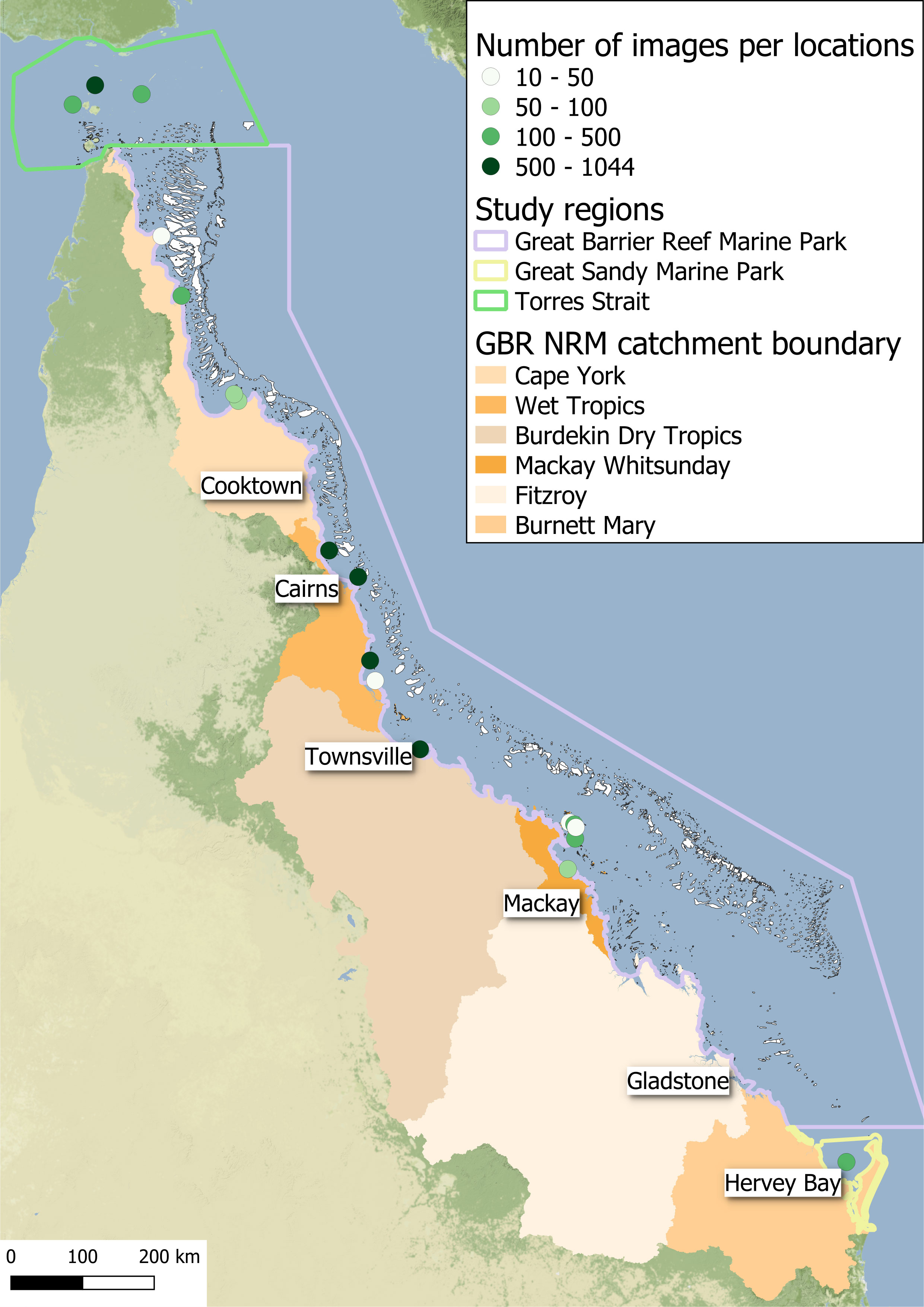
Figure 1 Map showing the location and number of images used for the Subtidal Seagrass Detector in the Torres Strait, the Great Barrier Reef World Heritage Area and Great Sandy Marine Park.

2.1.1 Seagrass presence detector (Model #1)

We defined seagrass presence as an area of the seafloor, also known as benthos, spatially dominated by seagrass, which we classed as ≥3% cover (sensu Mount et al., 2007). Images with seagrass cover less than 3% were excluded, resulting in the removal of an additional 819 images from the analysis. This maximised the power of detection to levels where seagrass was clearly visible. There were 1727 images with seagrass absent and 3236 with seagrass present. To ensure a balance dataset of the two classes, 1727 images were chosen at random out of the 3236 while ensuring the inclusion of all images from the minor seagrass morphology classes oval-shaped (522) and fernlike (165). The remaining images with seagrass present (1509) were retained for further testing.

2.1.2 Seagrass cover category classifier (Model #2)

Cover categories were first established based on four cover quantiles, which were equivalent to seagrass percent cover categories of; ≥3 <9%, ≥9 <15%, ≥15 <30% and ≥30%. However, the resulting model did not adequately distinguish between the two middle categories (less than 60% accuracy). Therefore, those two classes were merged resulting in three main classes used in Model #2: (1) low seagrass cover (≥3 <10%), (2) medium seagrass cover (≥10 <30%), and (3) high seagrass cover (≥30%) (Figure 2). The classes were somewhat unbalanced with 1082, 1509 and 644 images respectively. However, more images in the medium class were beneficial as it helped improve accuracy for that class which is the most commonly occurring at MMP sites (long term mean of 14% seagrass cover for coastal and reef subtidal sites where seagrass is present). When we ran the same model on a down-sampled version of the dataset (644 images for each class) the overall accuracy was lower (-3.3%): accuracy for the low and high cover class increased (+12.5% and +7.9% respectively), while the accuracy for the medium class significantly decreased (-26.3%).

FIGURE 2

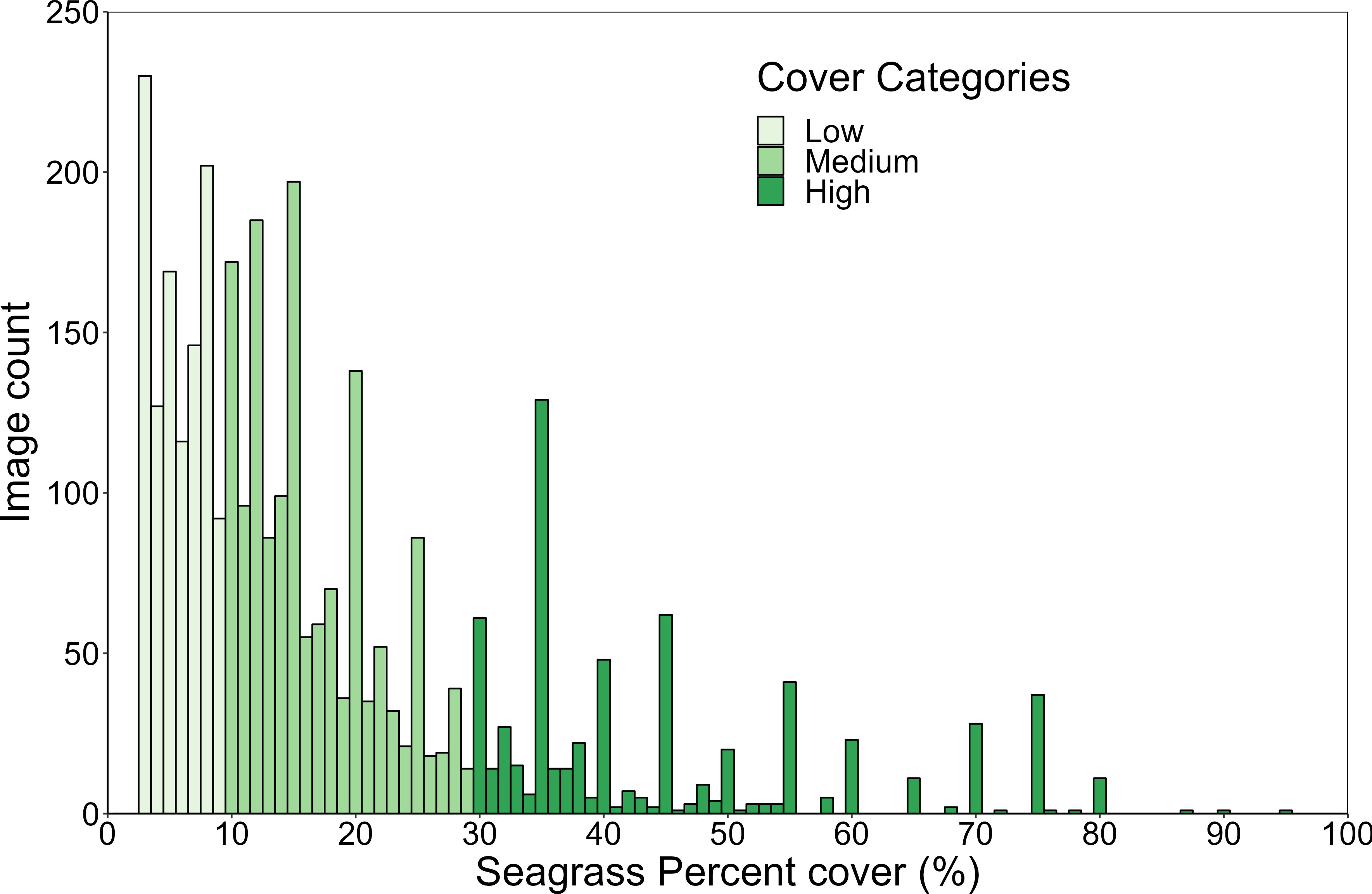
Figure 2 Distribution of seagrass percent cover in the image dataset used for Model #2.

2.1.3 Substrate complexity classifier (Model #3)

The substrate complexity classifier was applied to all images without any seagrass present. Those images were labelled either as ‘simple substrate’ or as ‘complex substrate’. The ‘simple’ category was assigned to clear images with mostly sandy bottoms while the ‘complex’ category was assigned to images that met at least one of the following conditions:

● had consolidated substrates, such as rock, live coral or coral rubble

● had a visually significant amount of macroalgae

● labelling was difficult (e.g. poor visibility, small seagrass species, poor image contrast).

Out of the 1727 images without seagrass, 1129 had simple substrate and 598 had complex substrate. Similar to Model #1, a random 531 simple substrate images were excluded and retained for further testing to unsure a balance dataset during training. This classifier can provide a potential reason for the absence of seagrass as well as highlighting potential shortfall in the seagrass detection from Model #1. In complex substrate habitats, seagrass could be present, however, percent cover is most likely to be low (<10%) and particularly difficult to detect by the model. Images predicted into this category can be later manually inspected to confirm the absence of seagrass.

All three final datasets were split 60-20-20 into a training, validation and test set.

2.2 Deep neural network modelling

2.2.1 Image classification workflow

Our overall aim for this study was to develop a Detector that would be able to achieve three separate classification tasks: (1) detect the presence/absence of seagrass, (2) estimate the seagrass cover (low, medium or high), and (3) identify the level of complexity of the substrate (simple or complex). Separate deep learning models were developed to execute each of these tasks independently which maximised model accuracy and reduced category imbalance (Figure 3). All model training and testing was conducted in Python using Keras (Chollet, 2015) on a local machine (Intel Core i9-10900KF CPU 3.70GHz, 3696 Mhz, 10 Cores, 20 Logical Processors, 64GB 3200 MHz, GPU NVIDIA GeForce RTX 3090).

FIGURE 3

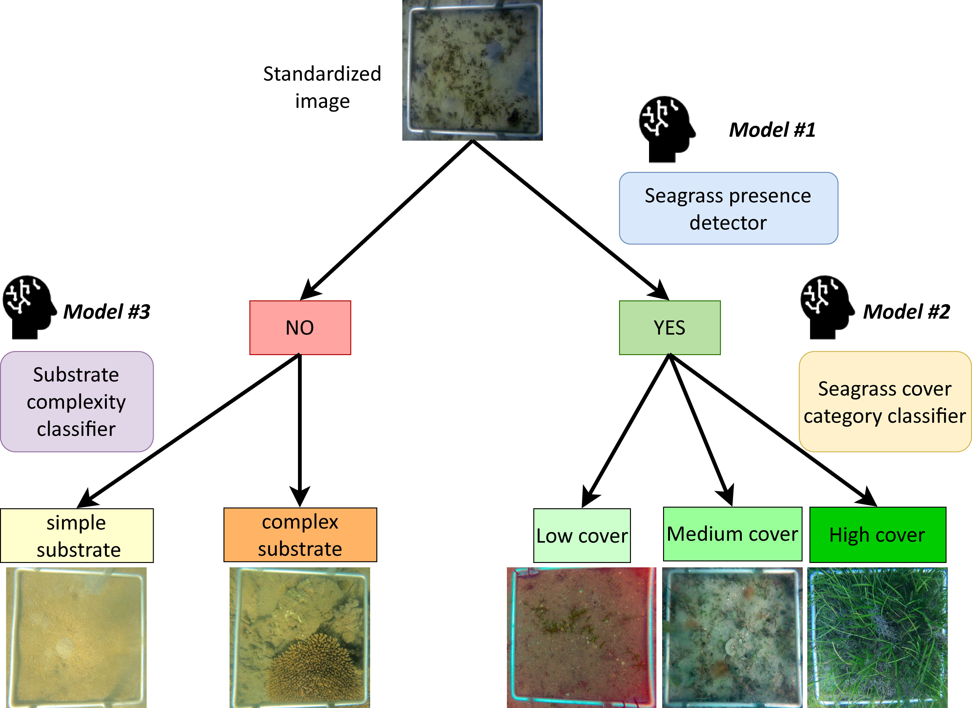
Figure 3 Diagram detailing the image classification workflow process of the Detector with the three deep learning models involved.

2.2.2 Model architecture

The classification models were composed of a binary classification model for Model #1 and Model #3 and multiclass classification for Model #2. The classification employed deep learning also known as DNNs. Training a neural network can be a protracted process and requires a large number of images to achieve satisfactory results. Transfer learning has been developed where an already successfully trained network such as VGG16 can be used as a feature extractor and coupled with a new classifier trained for the new specific task (Tammina, 2019). Our initial network was composed of a VGG16 model pre-trained on the ImageNet classification tasks (Zhang et al., 2015). Instead of the final dense layer from the original VGG16 model, we created our own custom classier composed of a sequence of two fully connected layers with 512 nodes and ReLU activation (Agarap, 2018), two consecutive dropout (Srivastava et al., 2014) with probability of 0.05 and 0.5 to prevent overfitting and a final dense layer with one node for each of predicted class activated by either the Sigmoid or Softmax function (Figure 4).

FIGURE 4

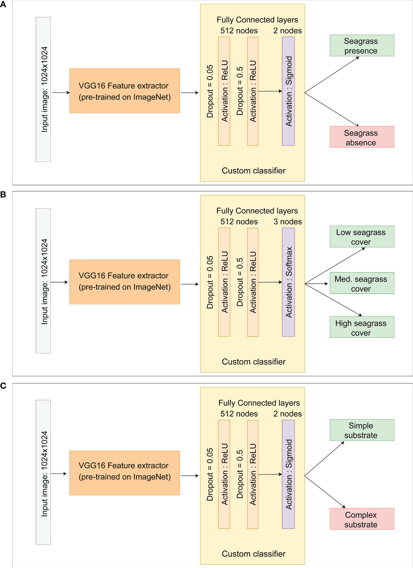
Figure 4 Convolution neural network architecture of: (A) Model #1, (B) Model #2 and (C) Model #3.

Contrary to other studies (Raine et al., 2020) we chose not to split our original images as it would have meant having to create new labels for thousands of sub-images. Instead, the input image size was increased. After multiple trials we found that optimal results were achieved for the input size of 1024x1024 pixels. We also tried more complex networks for feature extraction such as Resnet50 and EfficientNet but they did not perform as well overall (-1.7 and -5.2% in overall accuracy respectively).

2.2.3 Model training

The DNNs were all trained independently on batches of eight random images per training iteration. When the DNN has gone through as many iterations as needed to process the full training image set, this constituted an epoch. Throughout the whole training process, the progress of the learning is monitored by evaluating the model performance on the validation image set.

We started with an initial training phase where only the final classification layers (custom classifier part) were trainable and the rest of the VGG16 layers were frozen. During this phase the Adam optimizer (Kingma and Ba, 2014) was used with an initial learning rate of 0.001. If the loss on the validation image set did not improve after 10 epochs the learning rate was reduced by half up to four times after which the training was stopped. That process lasted 60 to 68 epochs. A fine-tuning training phase followed, where the VGG16 layers were unfrozen and set as trainable. This was done over 100 epochs and with the RMSprop optimizer (Tieleman and Hinton, 2014) and a much slower learning rate of 0.00001. The fine-tuning is meant to ensure the feature extraction is optimised for our input size as well as increasing performance of the models.

To further prevent overfitting and best capture, the potential illumination and turbidity variations of underwater images, colour-based data augmentation was applied where brightness (-70 to 70), contrast (0.1 to 0.3), blur (sigma 0 to 0.5) and the red channel (-50 to 50) were randomly altered at each training iteration.

2.2.4 Model evaluation (testing)

The training process stopped once all the DNNs have reached a plateau where further training did not further improve performances on the validation set.

We then conducted final evaluation of the model performances on the test image set (20% of the total) where accuracy was assessed in detail. For Model #1 and Model #3, further testing was conducted by running the model on the remaining images not included in the training, validation and test sets.

3 Results

3.1 Model #1

Model #1 achieved 97.0% accuracy (Supplementary Table S2) on the test image set (691). We had 3 false positive and 18 false negative classifications (Figure 5; Supplementary Table S3A). The false positives were all images from Low Isles and taken on SCUBA. We suspect that the presence of turf algae and the low image quality could be the source of the misclassification. The small number of false positives suggests the model was not overestimating seagrass presence.

FIGURE 5

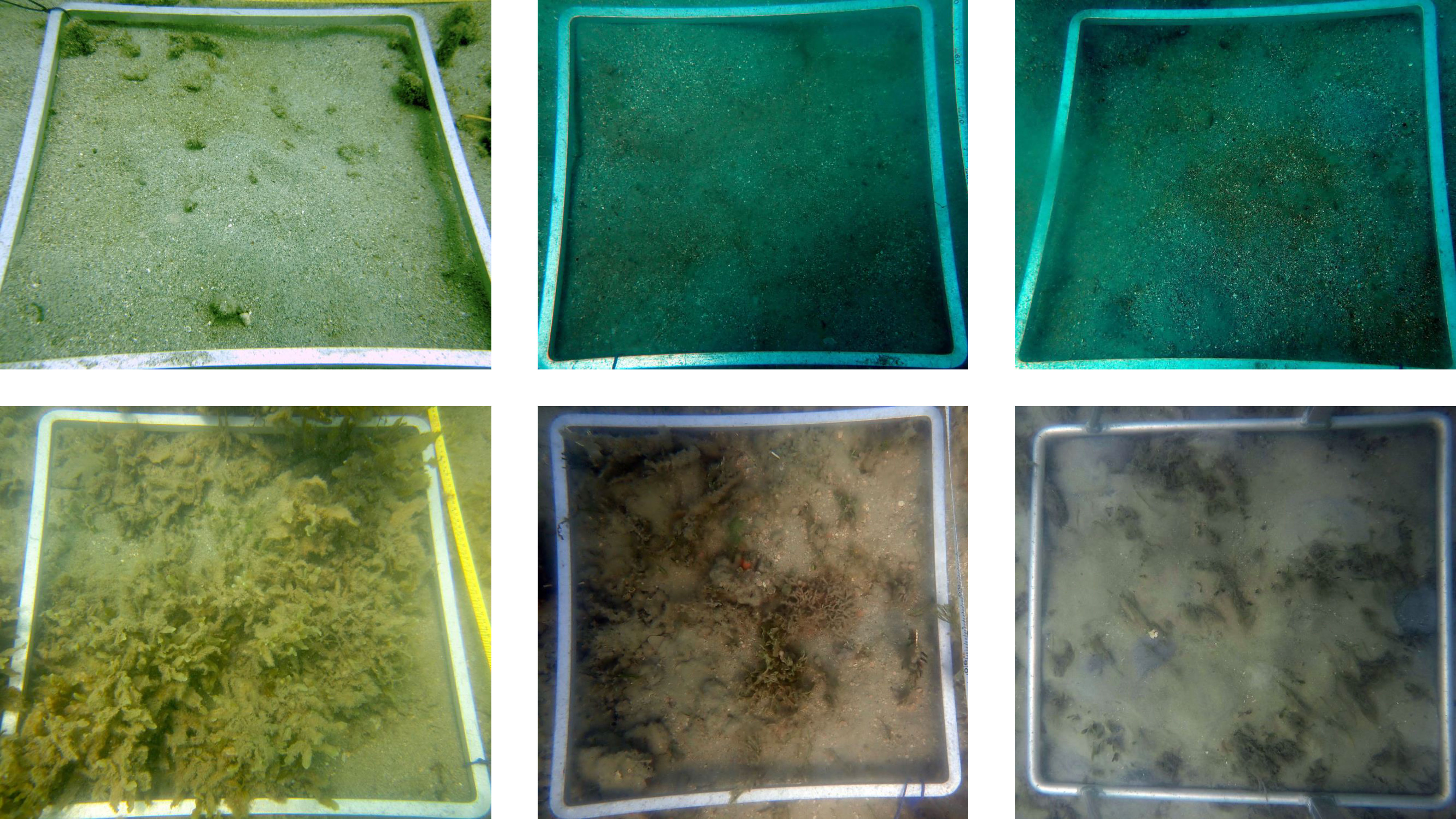
Figure 5 Examples of images misclassified by Model #1 with false positives on top row and false negative on the bottom row.

Of the false negative images, 16 had a percent cover lower than 10% and in nine of these percent cover was lower than 5% (Figure 6). In addition, 14 of the false negative images had a complex substrate with seven having more than 15% algae cover. This was further confirmed by running the model on the remaining seagrass photos not included in the training, validation and test sets. The model failed to detect seagrass in 38 out of 1509 images, achieving 97.4% accuracy. A similar pattern was observed where 31 of the misclassified images had less than 10% seagrass cover and 33 had complex substrate (Figure 6).

FIGURE 6

Figure 6 Histogram of the distribution of the seagrass percent cover and substrate complexity present in the images misclassified (false negative) by Model #1 from the test set (18) and the remaining seagrass photo set (38).

3.2 Model #2

Model #2 had an overall accuracy of 80.7% (Supplementary Table S2) on the test image set (647). The highest accuracy was achieved for the medium cover class (84.3%), followed by the low cover class (78.5%) and the high cover class (75.9%). However, these differences in accuracies were marginal and most likely a consequence of the unbalanced nature of the cover classes image dataset (Figure 7; Supplementary Table S3C).

FIGURE 7

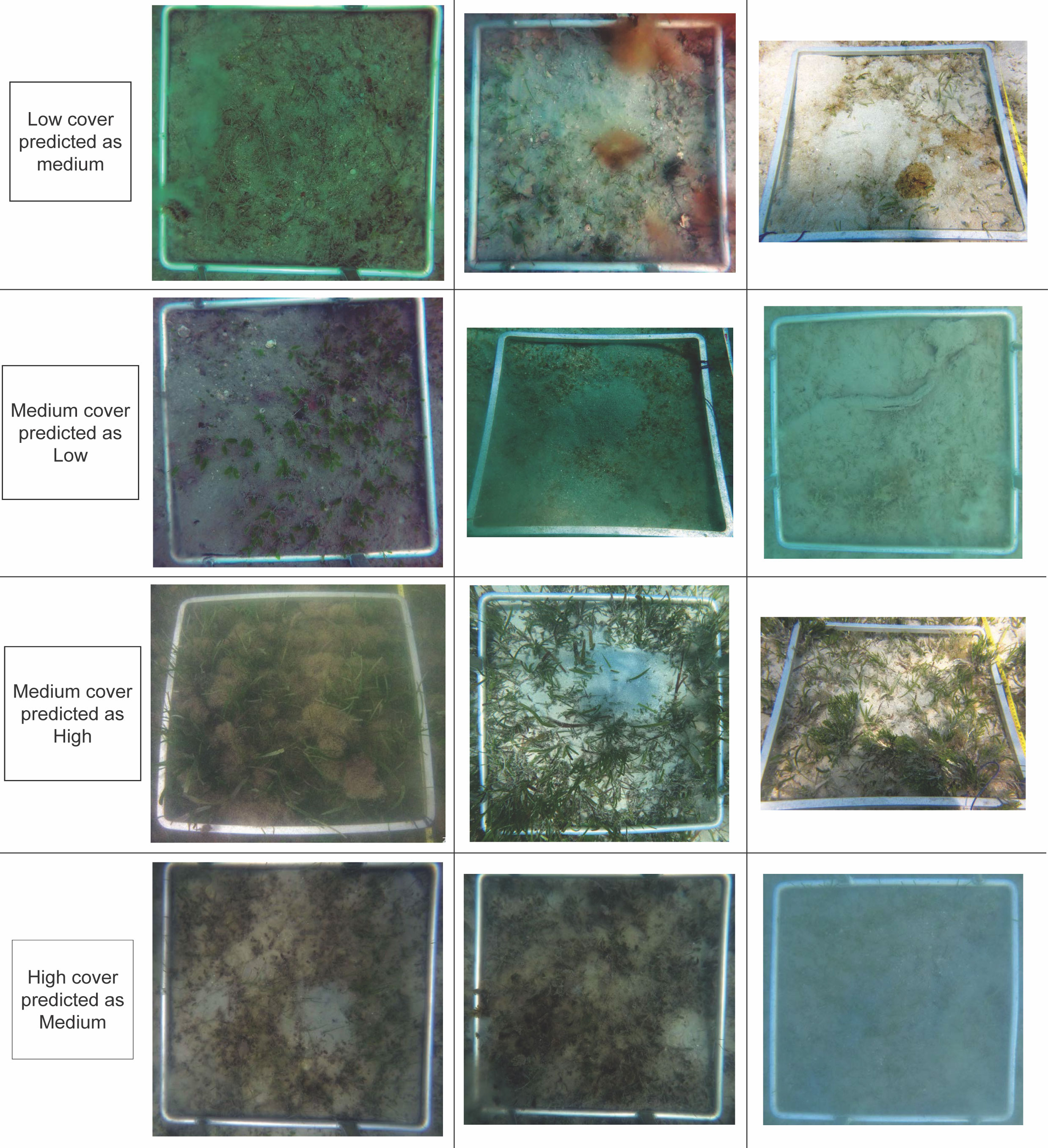
Figure 7 Examples of images misclassified by Model #2 from the low, medium and high cover categories.

All the misclassified images of the low cover classes (45) were incorrectly predicted to be in the medium cover category. Misclassification occurred for images with percent cover between 7 and 9% (31) (Figure 8A). Furthermore, 32 of which also had a complex substrate, further highlighting the difficulty categorising images close to the threshold of 10%, especially for complex substrates where algae for example could be biasing the predictions.

FIGURE 8

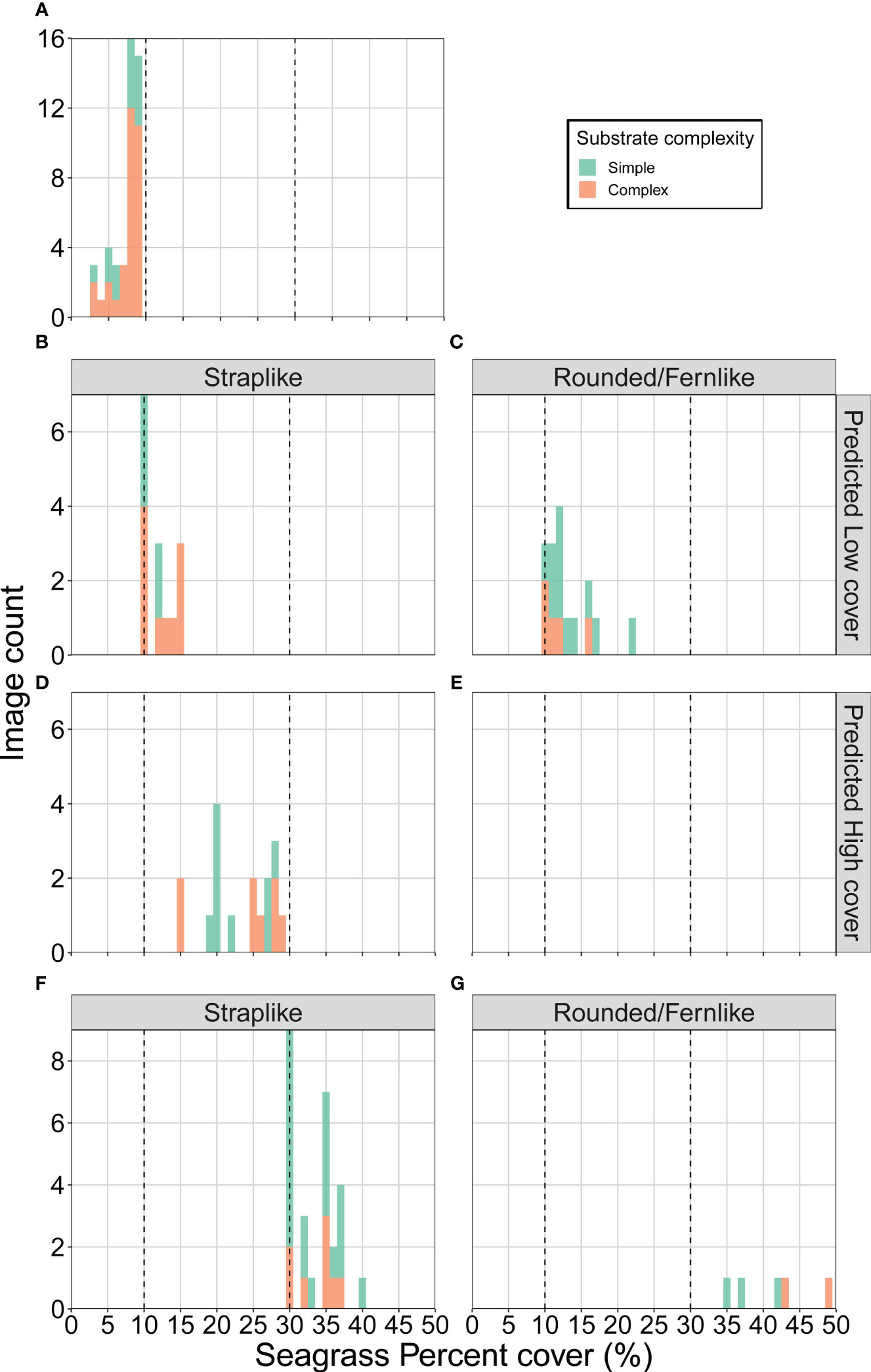
Figure 8 Histogram of the distribution of the seagrass percent cover and substrate complexity present in the misclassified images by Model #2 of (A) the low cover category (false medium), the medium cover category with (B, C) false low and (D, E) false high for straplike and rounded/fernlike species, and the high cover category (false medium) for (F) straplike and (G) rounded/fernlike.

There were 48 misclassified images of the medium cover classes, of which 31 were predicted as low cover and 17 as high cover. The false low cover images were mostly close to the 10% threshold with 27 of these images being between 10 and 15% seagrass cover (Figures 8B, C). Images dominated by smaller seagrass species with rounded and fernlike morphology were also a source of misclassification. The false high classifications were solely dominated by straplike species and 10 images had a seagrass cover between 20 and 30% (Figures 8D, E).

There were 32 misclassified images of the high cover class, which were all predicted as a medium cover. Similar to the previous classes, a vast majority of these were close to the adjacent cover category threshold with 28 of these images having less than 38% seagrass cover (Figures 8F, G). Straplike morphology dominated in 27 of the misclassified images except for those with percent cover of more than 40% which were dominated by rounded and fernlike morphology.

The type of substrate was not a significant driver of prediction errors for the medium and high cover class.

3.3 Model #3

Our subtidal substrate complexity classifier (Model #3) achieved an accuracy of 97.9% (Supplementary Table S2) on the test image set (240) and on the simple substrate only images remaining (531). There were two images misclassified as complex and three images were misclassified as simple instead of complex out of the test image set (Figure 9; Supplementary Table S3D). These images were also difficult to manually classify because they were mostly composed of a simple sandy substrate with some additional features such as algae or soft coral, or have poor visibility.

FIGURE 9

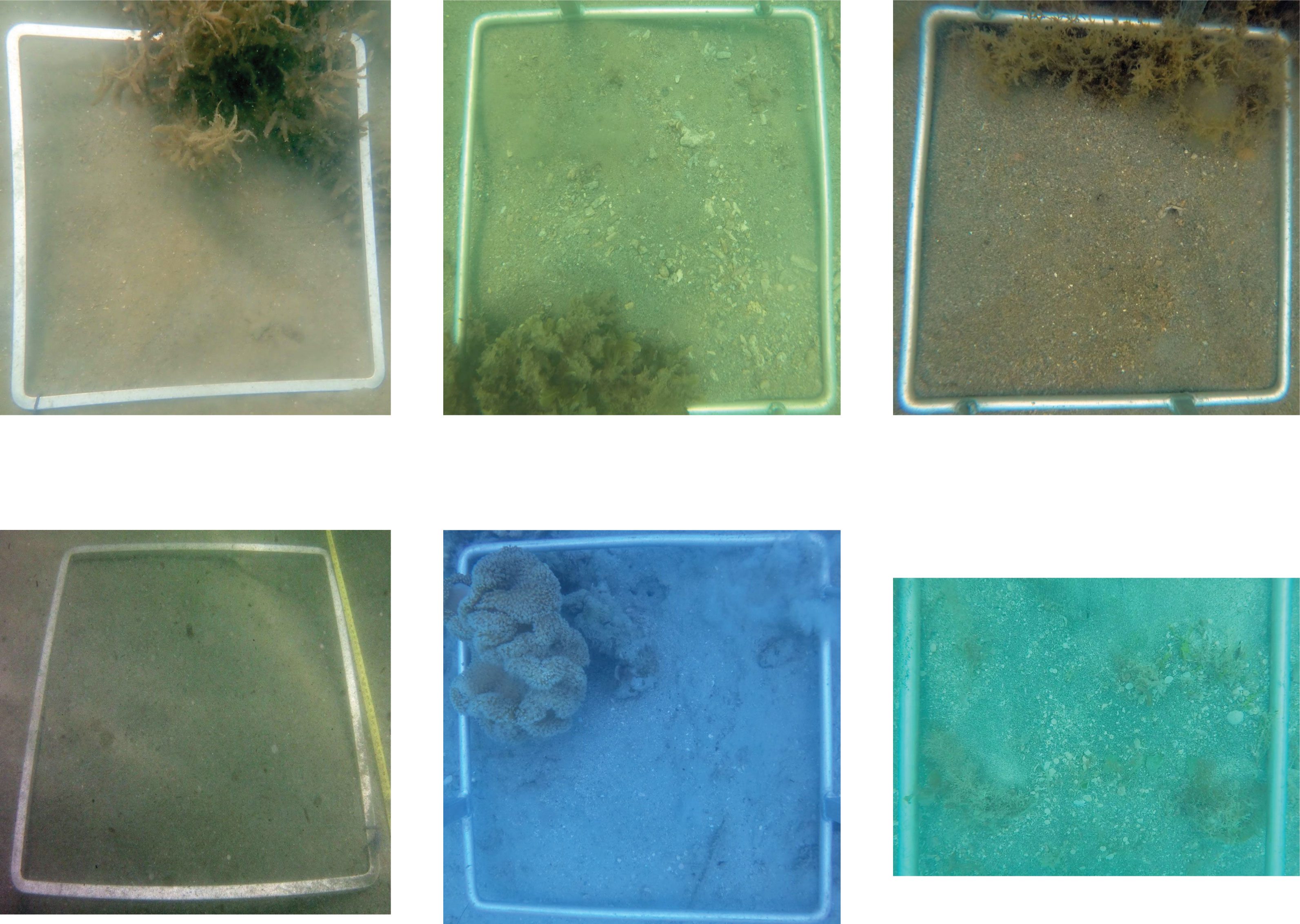
Figure 9 Examples of images misclassified by Model #3 with false complex on top row and false simple on the bottom row.

There were 11 images misclassified as complex instead of simple out of the simple substrate images remaining. These had 7% algae cover on average and 10 had more than 3%. This may be a consequence of the arbitrary binary classification used during the labelling process. It is very difficult to establish a clear difference between a quadrat with a simple sandy substrate with some algae or other features like coral and a complex substrate. These instances are uncommon within the dataset, with 82 images labelled as simple substrate and more than 3% algae cover and occurred mainly only at the Dunk Island and Low Isles sites (36 and 30 images respectively). This could be easily refined further by increasing the image dataset and by setting clearer thresholds or rules to define the substrate complexity classes.

4 Discussion

4.1 Method performance and limitation

The main goal of this research was to determine the potential for deep learning models to detect the presence of seagrass within underwater photos. Seagrass was identified in images containing a mix of seagrass species, seagrass morphologies and from a range of habitats/substrates with a very high level of accuracy (97%). This was achieved using a simple neural network architecture. The performance of Model #1 was higher than previously published deep learning seagrass detection models (Raine et al., 2020). However, a direct comparison between the accuracies is difficult due to differences in image dataset size and classifiers for seagrass morphology between studies.

We found that most of the misclassification occurred for images with complex substrate especially those with high algae percent cover. This is typical for deep learning classification models that are still lacking the ability to apply extreme generalization the way humans do (Chollet, 2017). Differentiating among well-defined objects is usually straight forward with numerous documented examples on image datasets such as ImageNet (Krizhevsky et al., 2017). The model outcomes for complex substrate, could possibly be improved by increasing the overall number of images, but also by having a balanced number of images with the same level of algae with and without seagrass. Indeed, deep learning models can continue to “learn” with additional imagery, so as new images are being collected, our models can be further trained which will lead to improved performance over time.

We also demonstrated it was possible to categorise seagrass cover into three broad classes with an accuracy of 80.7%. The choice of category boundaries was crucial in the model performance. Most of the classification errors happened around these boundaries and resulted in an image being placed into the adjacent category, rather than for example two categories away (i.e. a high being classed as low or vice versa). This needs to be considered when applying the model. For instance, the medium seagrass cover category was defined as ≥10 <30% during the labelling process, however the percent cover range of the images predicted in that class ranged from 7 to 35%. Despite these misclassification potential errors, using broad seagrass cover categories is sufficient in the context of mapping. At the scale of the photoquadrat used in this study, it is currently more accurate and easier to assess seagrass cover with a classification model rather than a regression model via segmentation of the image. Because of the very small morphology of the seagrass species in the Reef and the high level of complexity in the background (e.g. macroalgae, rubbles, turf algae), automated segmentation or even manual annotation of seagrass leaves is incredibly difficult in particular for strap-like species.

Seagrass percent cover estimates can be difficult to assign for low densities. Except for a few structurally large species, individual seagrass leaves are very small and therefore may not be easy to identify. A study from Moniruzzaman et al. (2019) developed deep learning models to detect single leaves of Halophila ovalis. This was effective for oblique close-up images with a sand background, but is likely to be less effective with nadir quadrat images as used in this study. Photoquadrats are used so that cover can be easily quantified in a standardised manner. While it would require a significant effort to label a photoquadrat dataset with individual bounding boxes, it might be the best way to detect very low seagrass density (<3%) and deserves further investigation.

An alternative method to estimate percent cover of benthic taxa (e.g. coral, algae, seagrass) and substrate (e.g. sand, rock) is using a point annotation system. This method has been successfully used for coral reefs and invertebrate communities (González-Rivero et al., 2016) and is publicly available through platforms such as CoralNet or ReefCloud. In seagrass habitats, the point annotation method is only able to detect seagrass when cover is above 25% (Kovacs et al., 2022). This is because the method relies on classifying an area (224x224 pixels) around the annotated point. The dimension of the annotation area is not visible through the labelling interface and the person conducting the labelling is expected to label only what is directly under the point. This approach is appropriate for well–defined and larger objects like coral, however, it is not well adapted to scattered, low and sparse seagrass cover where there could be seagrass within the classifying area but not directly under the point, resulting in a high level of misclassification. By classifying the patches directly, others studies have shown very high overall accuracy for multi-species seagrass detection (Raine et al., 2020) and even the addition of semi-supervised learning to reduce labelling effort (Noman et al., 2021). However, this was achieved on a dataset composed of images from Moreton Bay (Queensland, Australia), which does not encompass all species present within our study area and does not include complex substrate background.

While we acknowledge the limitations of our models, especially Model #2, we believe to have developed the most operationally relevant subtidal seagrass detection deep learning model for the Reef to date with a lot of potential for future improvements.

4.2 Operationalisation and mainstreaming

This study was undertaken to demonstrate the feasibility of a subtidal seagrass detection model as a step towards operationalisation and mainstreaming of big data acquisition and analysis (Dalby et al., 2021).

Traditional direct field observations provide instantaneous data, but need to be performed or overseen by formally trained scientists, and the data requires time consuming transcription into a database. Images (e.g. photoquadrats), however, can be collected by a variety of contributors such as environmental practitioners, Indigenous ranger groups or members of the public without a formal scientific background (i.e. citizen scientists), requiring less capacity and resources. For example, rangers from the Queensland Park and Wildlife Services (QPWS) conduct subtidal seagrass monitoring using drop cameras that is currently integrated into the MMP (Mckenzie et al., 2021). Citizen scientists, QPWS Rangers and Indigenous rangers frequently access the Reef and seagrass habitats of northern Australia. Simplifying the methods and minimising the time required to capture data by using photoquadrats can vastly increase the volume, velocity, variety and geographic spread of image data collection. The models presented in this study facilitate the ability to mainstream data capture and increase the rate of image processing, enabling scientists to maximise big data analysis and reporting. With our current computer, the models are able to process and produce predictions for 1500 images in under two minutes. In our experience it would take approximately 12 to 25 hours for a trained person to manually label that number of images depending on their complexity. Scaling up the process will require some specific infrastructure to store data and powerful cloud computing capacity (CPU and GPU) on platforms such as AWS or Azure to handle on-demand inference of new data. In addition of the deep learning models, we aim to grow our capacity for image data handling. In parallel with the development of the models presented here we have been working on streamlining a higher efficiency image processing workflow. This includes handling either time-lapse or video (e.g. GoPro) input sources and a DDN model (YOLOv5) to generate deep learning ready standardized quadrat images via detecting quadrat metal frame and cropping the image.

The operational applications for the subtidal seagrass detector are wide-ranging, including mapping and monitoring of the vast and remote northern Australian and global seagrass habitats. Image collection combined with a geotagging/geolocation, will enable the production of spatially explicit maps of subtidal areas. Our models are most adapted to this application as maps tend to only need simple information like seagrass presence/absence. However, we have also shown potential for monitoring with the ability to detect broad seagrass cover categories which with further refinement could enable temporal changes in seagrass abundance to be assessed.

4.3 Future directions

While the findings in this study are encouraging, we very much intend to further refine and improve those models and the associated data processing workflow over time. One of the main advantages of using DNNs is their capacity to incrementally improve when additional training data is provided. Therefore, as more and more diverse images are supplied it will help us build more robust models and give greater confidence in the predictions. Our models are currently limited to be used on subtidal nadir photoquadrats captured using a drop-camera. However, with the increasing popularity of Autonomous Underwater Vehicles (AUVs), our DNNs would need to be trained to accept more versatile image inputs (e.g. oblique and without guiding bounds).

5 Conclusion

In this study, we developed a Subtidal Seagrass Detector capable of detecting the presence of seagrass as well as classifying seagrass cover and substrate complexity in underwater photoquadrats by using Deep Neural Networks. The three subsequent models achieved high level accuracies with 97%, 80.7% and 97.9%, respectively. This demonstrates great potential towards the operationalisation of the Detector for accurate automated seagrass detection over a wide range of subtidal seagrass habitats.

Data availability statement

The raw data supporting the conclusions of this article will be made available by the authors, without undue reservation.

Author contributions

Conceptualisation, LL, CC and LM. Methodology, LL, CC and LM. Validation, LL, CC and LM. Formal analysis, LL. Investigation, LL, CC and LM. Resources, LL, CC and LM. Data curation, LL. Writing—original draft preparation, LL, CC and LM. Writing—review and editing, LL, CC and LM. Visualisation, LL, CC and LM. All authors contributed to the article and approved the submitted version.

Funding

This research was internally funded by the Centre for Tropical Water and Aquatic Ecosystem Research (TropWATER), James Cook University, Cairns, QLD, Australia.

Acknowledgments

We thank Rudi Yoshida, Haley Brien, Abby Fatland, Jasmina Uusitalo and Miwa Takahashi assistance with data collection. We acknowledge the Australian Government and the Great Barrier Reef Marine Park Authority (the Authority) for support of the collection of the Great Barrier Reef data under the Marine Monitoring Program. We thank Sascha Taylor and the QPWS rangers who conducted the subtidal drop camera field assessments in Cape York, southern Wet Tropics and Mackay–Whitsunday regions of the Great Barrier Reef. Torres Strait seagrass images were collected by the Sea Team of the Land and Sea Management Unit as part of seagrass monitoring funded by Torres Strait Regional Authority. We thank Damien Burrows for his support for this research and Mohammad Jahanbakht for help reviewing the manuscript. We also thank all Traditional Owners of the sea countries we visited to conduct our research: Wuthathi, Uutaalnganu, Yiithuwarra, Eastern Kuku Yalanji, Gunggandji, Djiru, Bandjin, Wulgurukaba, Ngaro, Gia and Butchulla. Parts of this manuscript has been released as a technical report at TropWATER, (Langlois et al., 2022).

Conflict of interest

The authors declare that the research was conducted in the absence of any commercial or financial relationships that could be construed as a potential conflict of interest.

Publisher’s note

All claims expressed in this article are solely those of the authors and do not necessarily represent those of their affiliated organizations, or those of the publisher, the editors and the reviewers. Any product that may be evaluated in this article, or claim that may be made by its manufacturer, is not guaranteed or endorsed by the publisher.

Supplementary material

The Supplementary Material for this article can be found online at: https://www.frontiersin.org/articles/10.3389/fmars.2023.1197695/full#supplementary-material

References

Agarap A. F. (2018). Deep learning using rectified linear units (ReLU). arXiv. doi: 10.48550/arxiv.1803.08375

CrossRef Full Text | Google Scholar

Balado J., Olabarria C., Martínez-Sánchez J., Rodríguez-Pérez J. R., Pedro A. (2021). Semantic segmentation of major macroalgae in coastal environments using high-resolution ground imagery and deep learning. Int. J. Remote Sens. 42, 1785–1800. doi: 10.1080/01431161.2020.1842543

CrossRef Full Text | Google Scholar

Beijbom O., Edmunds P. J., Roelfsema C., Smith J., Kline D. I., Neal B. P., et al. (2015). Towards automated annotation of benthic survey images: variability of human experts and operational modes of automation. PloS One 10, e0130312. doi: 10.1371/journal.pone.0130312

PubMed Abstract | CrossRef Full Text | Google Scholar

Carter A. B., Collier C., Lawrence E., Rasheed M. A., Robson B. J., Coles R. (2021a). A spatial analysis of seagrass habitat and community diversity in the great barrier reef world heritage area. Sci. Rep. 11, 22344. doi: 10.1038/s41598-021-01471-4

PubMed Abstract | CrossRef Full Text | Google Scholar

Carter A. B., David M., Whap T., Hoffman L. R., Scott A. L., Rasheed M. A. (2021b). Torres Strait seagrass 2021 report card. TropWATER report no. 21/13 (Cairns: TropWATER, James Cook University).

Google Scholar

Carter A. B., Mckenna S. A., Rasheed M. A., Collier C., Mckenzie L., Pitcher R., et al. (2021c). Synthesizing 35 years of seagrass spatial data from the great barrier reef world heritage area, Queensland, Australia. Limnol. Oceanogr. Lett. 6, 216–226. doi: 10.1002/lol2.10193

CrossRef Full Text | Google Scholar

Chollet F. (2015). keras, GitHub. Available at: https://github.com/fchollet/keras.

Google Scholar

Chollet F. (2017). Deep learning with python (Shelter Island, NY: Manning Publications).

Google Scholar

Dalby O., Sinha I., Unsworth R. K. F., Mckenzie L. J., Jones B. L., Cullen-Unsworth L. C. (2021). Citizen science driven big data collection requires improved and inclusive societal engagement. Front. Mar. Sci. 8. doi: 10.3389/fmars.2021.610397

CrossRef Full Text | Google Scholar

González-Rivero M., Beijbom O., Rodriguez-Ramirez A., Holtrop T., González-Marrero Y., Ganase A., et al. (2016). Scaling up ecological measurements of coral reefs using semi-automated field image collection and analysis. Remote Sens. 8, 30. doi: 10.3390/rs8010030

CrossRef Full Text | Google Scholar

Johnson J. E., Welch D. J., Marshall P., Day J., Marshall N., Steinberg C., et al. (2018). Characterising the values and connectivity of the northeast Australia seascape: great barrier reef, Torres strait, coral Sea and great sandy strait. report to the national environmental science program (Cairns: Rainforest Research Centre Limited).

Google Scholar

Kingma D. P., Ba J. (2014). Adam: A method for stochastic optimization. arXiv. doi: 10.48550/arxiv.1412.6980

CrossRef Full Text | Google Scholar

Kovacs E. M., Roelfsema C., Udy J., Baltais S., Lyons M., Phinn S. (2022). Cloud processing for simultaneous mapping of seagrass meadows in optically complex and varied water. Remote Sens. 14, 609. doi: 10.3390/rs14030609

CrossRef Full Text | Google Scholar

Krizhevsky A., Sutskever I., Hinton G. E. (2017). ImageNet classification with deep convolutional neural networks. Commun. ACM 60, 84–90. doi: 10.1145/3065386

CrossRef Full Text | Google Scholar

Langlois L. A., Collier C. J., Mckenzie L. J. (2022). Subtidal seagrass detector: development and preliminary validation (Cairns: Centre for Tropical Water & Aquatic Ecosystem Research, James Cook University). Available at: https://bit.ly/3WqYAQN.

Google Scholar

Mckenzie L. J., Campbell S. J., Roder C. A. (2003). Seagrass-watch: manual for mapping & monitoring seagrass resources (Cairns: QFS, NFC).

Google Scholar

Mckenzie L. J., Collier C., Langlois L., Yoshida R., Smith N., Waycott M. (2015). Reef rescue marine monitoring program - inshore seagrass, annual report for the sampling period 1st June 2013 – 31st may 2014 (Cairns: TropWATER, James Cook University).

Google Scholar

Mckenzie L. J., Collier C. J., Langlois L. A., Yoshida R. L., Uusitalo J., Waycott M. (2021). Marine monitoring program: annual report for inshore seagrass monitoring 2019–20 (Townsville, Australia: James Cook University).

Google Scholar

Mckenzie L. J., Collier C. J., Langlois L. A., Yoshida R. L., Waycott M. (2022a). Marine monitoring program: annual report for inshore seagrass monitoring 2020–21. report for the great barrier reef marine park authority (Townsville: Great Barrier Reef Marine Park Authority).

Google Scholar

Mckenzie L. J., Langlois L. A., Roelfsema C. M. (2022b). Improving approaches to mapping seagrass within the great barrier reef: from field to spaceborne earth observation. Remote Sens. 14, 2604. doi: 10.3390/rs14112604

CrossRef Full Text | Google Scholar

Mckenzie L. J., Nordlund L. M., Jones B. L., Cullen-Unsworth L. C., Roelfsema C., Unsworth R. K. F. (2020). The global distribution of seagrass meadows. Environ. Res. Lett. 15, 074041. doi: 10.1088/1748-9326/ab7d06

CrossRef Full Text | Google Scholar

Mckenzie L. J., Roder C. A., Roelofs A. J., Lee Long W. J. (2000). “Post-flood monitoring of seagrasses in hervey bay and the great sandy strait 1999: implications for dugong, turtle and fisheries management,” in Department of primary industries information series QI00059 (Cairns: Queensland Department of Primary Industries, NFC).

Google Scholar

Moniruzzaman M., Islam S. M. S., Lavery P., Bennamoun M. (2019). “Faster r-CNN based deep learning for seagrass detection from underwater digital images,” in 2019 digital image computing: techniques and applications (DICTA) (Perth, WA, Australia), 1–7. doi: 10.1109/DICTA47822.2019.8946048

CrossRef Full Text | Google Scholar

Mount R., Bricher P., Newton J. (2007). National Intertidal/Subtidal benthic (NISB) habitat classification scheme, version 1.0, October 2007 (Hobart, Tasmania: National Land & Water Resources Audit & School of Geography and Environmental Studies, University of Tasmania).

Google Scholar

Noman M. K., Islam S. M. S., Abu-Khalaf J., Lavery P. (2021). “Multi-species seagrass detection using semi-supervised learning,” in 2021 36th International Conference on Image and Vision Computing New Zealand (IVCNZ) (Tauranga, New Zealand). 1–6. doi: 10.1109/IVCNZ54163.2021.9653222

CrossRef Full Text | Google Scholar

Preen A. R., Lee Long W. J., Coles R. G. (1995). Flood and cyclone related loss, and partial recovery, of more than 1000 km2 of seagrass in hervey bay, Queensland, Australia. Aquat. Bot. 52, 3–17. doi: 10.1016/0304-3770(95)00491-H

CrossRef Full Text | Google Scholar

Raine S., Marchant R., Moghadam P., Maire F., Kettle B., Kusy B. (2020). Multi-species seagrass detection and classification from underwater images. Computer Vision and Pattern Recognition. doi: 10.1109/DICTA51227.2020.9363371

CrossRef Full Text | Google Scholar

Reus G., Möller T., Jäger J., Schultz S. T., Kruschel C., Hasenauer J., et al. (2018). “Looking for seagrass: deep learning for visual coverage estimation,” in 2018 OCEANS - MTS/IEEE Kobe Techno-Oceans (OTO) (Kobe, Japan). 1–6. doi: 10.1109/OCEANSKOBE.2018.8559302

CrossRef Full Text | Google Scholar

Schröder S.-M., Kiko R., Koch R. (2020). MorphoCluster: efficient annotation of plankton images by clustering. arXiv. doi: 10.48550/arxiv.2005.01595

CrossRef Full Text | Google Scholar

Seagrass-Watch (2022) Hervey bay (Clifton Beach: Seagrass-Watch Ltd). Available at: https://www.seagrasswatch.org/burnettmary/#HV (Accessed 22 June 2022).

Google Scholar

Sheaves M., Bradley M., Herrera C., Mattone C., Lennard C., Sheaves J., et al. (2020). Optimizing video sampling for juvenile fish surveys: using deep learning and evaluation of assumptions to produce critical fisheries parameters. Fish Fish. 21, 1259–1276. doi: 10.1111/faf.12501

CrossRef Full Text | Google Scholar

Srivastava N., Hinton G., Krizhevsky A., Sutskever I., Salakhutdinov R. (2014). Dropout: a simple way to prevent neural networks from overfitting. J. Mach. Learn. Res. 15, 1929–1958. doi: 10.5555/2627435.2670313

CrossRef Full Text | Google Scholar

Tammina S. (2019). Transfer learning using VGG-16 with deep convolutional neural network for classifying images. Int. J. Sci. Res. Publications (IJSRP) 9(10). doi: 10.29322/IJSRP.9.10.2019.p9420

CrossRef Full Text | Google Scholar

Tieleman T., Hinton G. (2014)RMSprop gradient optimization. Available at: http://www.cs.toronto.edu/tijmen/csc321/slides/lecture_slides_lec6.pdf.

Google Scholar

Zhang X., Zou J., He K., Sun J. (2015). Accelerating very deep convolutional networks for classification and detection. Computer Vision and Pattern Recognition. doi: 10.48550/arXiv.1505.06798

CrossRef Full Text | Google Scholar