Decadal variability of oxygen uptake, export, and storage in the Labrador Sea from observations and CMIP6 models

1 Introduction

The Labrador Sea is one of the few regions in the world where oxygen can be transported directly into the deep ocean, which acts as a supply for marine organisms throughout the global oceans. This supply of dissolved oxygen to the deep is the result of oxygen uptake through air-sea gas exchange (Atamanchuk et al., 2020), and its subsequent export out of the region (Koelling et al., 2022). Oxygen uptake occurs primarily during wintertime, when the process of deep convection continually mixes the water column to depths of more than 1000 m, bringing up low-oxygen water from below and maintaining an undersaturation of surface waters relative to the atmosphere (Wolf et al., 2018). The resulting air-sea gradient in oxygen, along with bubble injection driven by strong winds and wave breaking, leads to intense air-sea exchange of oxygen during these winter months (Koelling et al., 2017). As a result the Labrador Sea, and the subpolar North Atlantic as a whole, feature some of the strongest oxygen uptake rates anywhere in the world ocean (Huang et al., 2018), with annual values in the Labrador Sea being on the order of 20 mol m^–2 y^–1 (Atamanchuk et al., 2020). Thanks to this strong uptake and its link to deep water formation, the subpolar North Atlantic, along with the Southern Ocean, is the main region where oxygen can enter the deep ocean, making it one of the “lungs of the ocean” (Körtzinger et al., 2004; Portela et al., 2020). North Atlantic Deep Water (NADW), a water mass formed in part as a result of deep convection in the Labrador Sea, can be traced by its high oxygen concentrations in the formation region which decrease along southward spreading pathways (Figure 1). The formation of NADW in the subpolar North Atlantic also leads to a stark difference in mean oxygen concentration between the Atlantic Ocean and the Pacific and Indian Oceans.

FIGURE 1

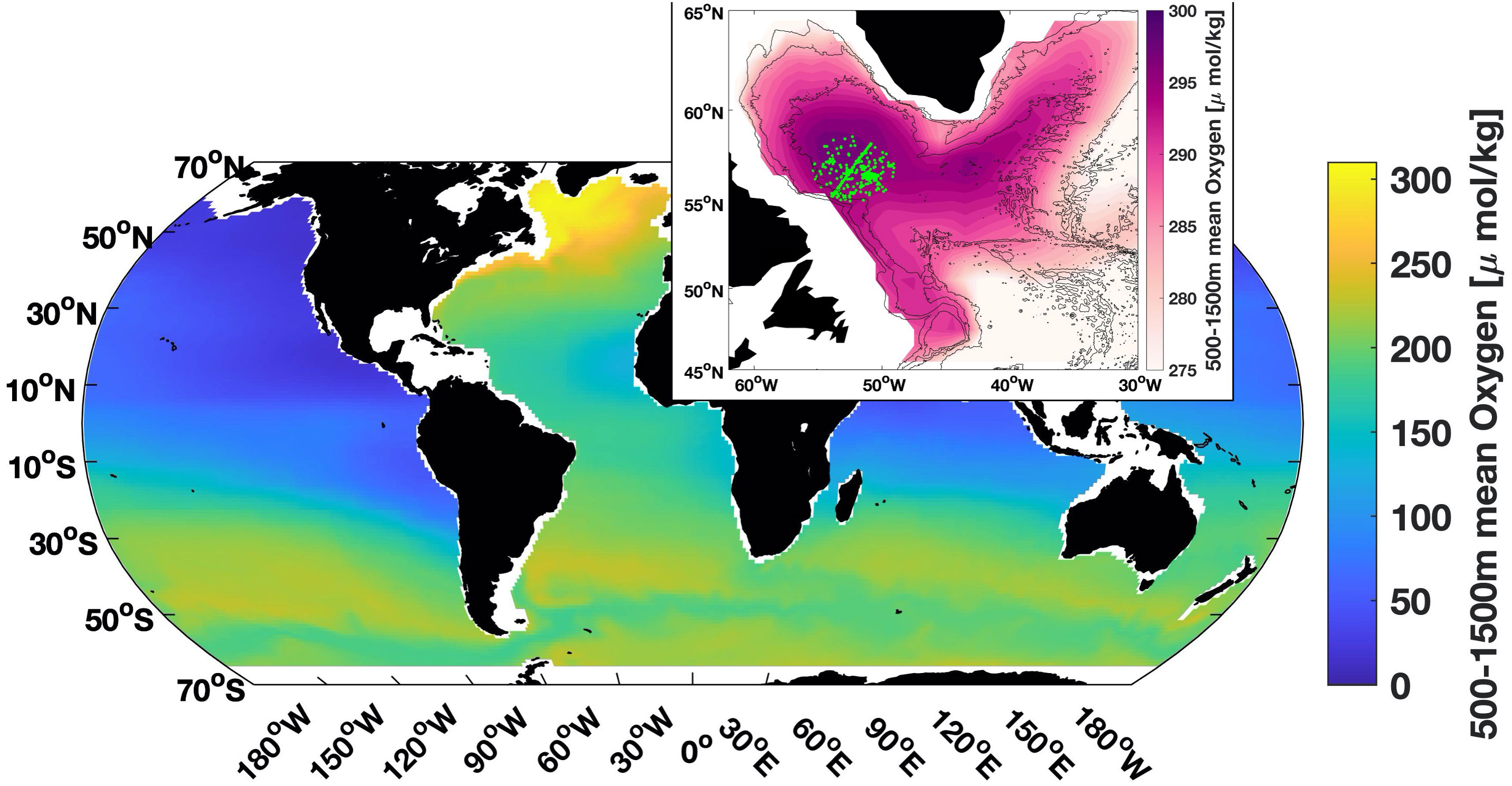
Figure 1 Global mean dissolved oxygen concentration between 500–1500 m depth from the GOBAI-O₂ gridded oxygen product (Sharp et al., 2022). Inset shows detail in the Labrador Sea, with green symbols representing measurements used to construct the time series in Figure 2.

The Labrador Sea has been sampled more consistently than most open ocean regions over many decades, with regular measurements dating back to the late 1940s. Furthermore, the main convection region in the interior Labrador Sea is relatively small and homogeneous, such that individual measurements at only a few stations can give useful information about variability in the basin (van Aken et al., 2011; Yashayaev and Loder, 2016). Ocean Weather Ship Bravo was stationed in the center of the basin from the 1940s to 1970s, and following occasional cruises in the 1950s to 1980s, the AR7W line across the basin from Labrador to Greenland has been occupied almost every year since 1987 as part of the WOCE, CLIVAR and AZOMP initiatives (Kieke and Yashayaev, 2015). The comprehensive record of oceanographic variables collected by these projects has been used primarily in the context of the variability in physical properties, and their relation to deep convection and the Atlantic Meridional Overturning Circulation (AMOC) (Yashayaev, 2007; Yashayaev and Loder, 2016). Fewer studies have focused on the variability in oxygen concentrations, with notable exceptions including studies by Stendardo and Gruber (2012) and van Aken et al. (2011) that reported long-term oxygen trends and variability in the subpolar North Atlantic until 2010 from the historic shipboard data, and Rhein et al. (2017) who analyzed variability in oxygen concentrations since the early 1990s. Here, we utilize the data to construct a time series of oxygen content anomalies for the Labrador Sea Water (LSW) layer (0–2200 m) in the central Labrador Sea from 1950 to 2015. We use this time series to discuss how the decadal-scale variability of oxygen concentrations reported in previous studies relates to variability in the uptake of oxygen during deep convection and its subsequent export along NADW spreading pathways.

Changes in the strength of ocean ventilation have been proposed as one of the reasons for widespread global ocean deoxygenation observed in recent decades (Ito et al., 2017; Schmidtko et al., 2017). However, this is not reproduced accurately in climate models, which feature too little deoxygenation particularly in the deep ocean, which may be related to difficulties with representing the processes underlying ventilation (Oschlies et al., 2017; Oschlies et al., 2018; Buchanan and Tagliabue, 2021). To assess the ability of climate models to reproduce observed variability in oxygen ventilation in the Labrador Sea, we use the time series constructed from observational data to evaluate nine different models that participated in the Ocean Model Intercomparison Project phase 1 component of the Climate Model Intercomparison Project phase 6 (hereinafter CMIP6-OMIP1). For this purpose, we develop a “model score” based on the ability of CMIP6-OMIP1 models to reproduce the observed variability in the oxygen content time series and mean profile from the WOD data, as well as gas exchange estimates taken from other studies. This score serves as a simplified metric of the ability of climate models to represent the complex processes that underlie ocean ventilation. Our assessment highlights processes which need to be better resolved in climate models in order to more accurately portray oxygen cycling in the Labrador Sea. This analysis could inform improvements for future model generations, and may be applicable to other regions with comparable dynamics.

Finally, we combine our analysis of the long-term variability in oxygen content with insights from previous observational studies of air-sea gas exchange and oxygen export, and with the CMIP6-OMIP1 model data, in order to understand how air-sea gas exchange, oxygen storage, and oxygen export are related on interannual and decadal time scales.

2 Materials and methods

2.1 Observational time series

To construct the oxygen inventory time series, we use quality controlled data from the World Ocean Database [WOD; Boyer et al. (2013)] in the central Labrador Sea, which includes oxygen measurements from as early as the 1950s. Some data from individual cruises are available as far back as 1927, but given the large temporal gaps these are not used in our study. We use all measurements within a 200 km radius of 56°49.3’N, 52°13.2’W from fixed platforms and shipboard hydrography, which are flagged as “good data” in the WOD (see Figure 1 for location). The data were averaged into annual values with 50 m vertical bins, and cover the period from 1950 to 2015. We chose not to include more recent data from profiling floats such as BGC-Argo in order to avoid biases resulting from the shift of predominantly ship-based data typically collected during spring or summer to predominantly autonomous data collected year-round. Even with the shipboard data, there may be some biases resulting from changing sampling schemes and times between years, particularly in the early parts of the record, as well as year-to-year variability associated with instrumental errors during individual cruises (Yashayaev et al., 2021). However, the focus here is on the longer-term decadal signals rather than variability from one year to the next, and we assume these effects are small compared to the decadal variability in properties, consistent with previous studies (van Aken et al., 2011). To further test the representativeness of a single point and data collected once a year for measuring interannual variability in the whole region, we used CMIP6-OMIP1 model output to construct a synthetic time series derived from one grid point in the center of the convection region once a year and compared it to the full time series using all data within a 200 km radius (Figure S1). The comparison suggests that taking measurements only at one location during summer each year does not introduce any significant bias.

To construct the time series of oxygen content anomalies, the time-mean oxygen profile was first subtracted from the annual WOD profiles, and the resulting anomalies were interpolated vertically between measurements, and extrapolated to the surface and seafloor, omitting years where no measurements were available below 2000 m. The anomalies were then integrated over the 0–2200 m depth range to obtain a time series of annual oxygen content anomalies in this depth range which we assume to be the maximum depth typically occupied by Labrador Sea Water (Yashayaev and Loder, 2016). The time series used for further analysis and comparison with the CMIP6-OMIP1 data was constructed by smoothing the annual time series with a 3-year running mean filter to reduce some of the noise associated with the sampling issues discussed above, and then filling any remaining gaps in the data with linear interpolation.

To estimate the uncertainty of the time series, we first calculated the standard deviation σ in each one-year, 50 m depth bin. These annual values were then averaged to obtain a mean standard deviation profile for the entire record as an approximation of the true statistical standard deviation. The standard error was calculated from this mean profile and the number of observations in each bin as ${\sigma }_{\overline{x}}=\frac{\sigma }{\sqrt{N}}$. Bins with no measurements were treated as having N = 1, i.e. the standard error is equal to the standard deviation. This method was chosen to avoid underestimating the error in years with fewer observations, where the standard deviation of the samples will be lower than the true standard deviation of the statistical population. The resulting error estimate for the oxygen inventory ranges from 1.59 mol m^–2 for recent years with more extensive coverage to 9.65 mol m^–2 for years with limited or no measurements.

2.2 CMIP6-OMIP1 models

To evaluate the processes governing the oxygen budget in the Labrador Sea, we also used data from nine ocean models that were part of the Coupled Model Intercomparison Project phase 6 (CMIP6), accessed from https://esgf-node.llnl.gov/search/cmip6/. The models selected were those that participated in phase 1 of the ocean model intercomparison project (OMIP1) and included a biogeochemical component (Orr et al., 2017) with monthly output of the variables of interest. The resulting selection of models was CCC CanESM5, CMCC ESM2, CNRM ESM2-1, IPSL CM6A-LR, MIROC E2SL, MRI ESM2.0, NCAR CESM2, NCC NorESM-LM, and NOAA GFDL-CM4, and we used the r1i1p1f1 variant where available, or the lowest number variant otherwise, as listed in Table 1. The model outputs used for the calculations are oxygen concentration (variable name o2), and surface air-sea gas exchange of oxygen (variable name fgo2). The time period considered in this study is 1950–2009, which is the window overlapping with the period of consistent observational data (1950–2015), and also coincides with almost a full cycle of the 1948–2009 CORE-II atmospheric forcing (Large and Yeager, 2009) that is used in all OMIP1 runs (Orr et al., 2017). Based on the comparison in Figure S1 we use data from a single grid point in the center of the convection region to be representative of the convective patch.

TABLE 1

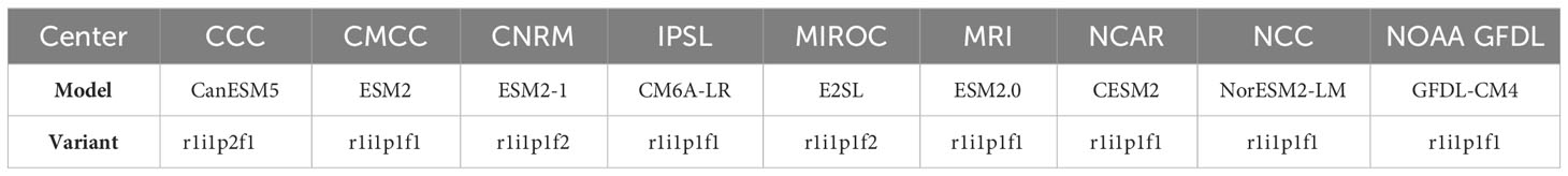
Table 1 Summary of models used in this study. All model runs used are OMIP1.

2.3 Oxygen budget calculation

As a biologically active element, the change in the inventory of oxygen for a given volume of the open ocean is controlled by both physical processes, such as air-sea gas exchange, lateral advection, and vertical export, and net community metabolism, which represents the net effect of biological production minus autotrophic and heterotrophic respiration (Martz et al., 2009; Koelling et al., 2017).

$\begin{array}{ll}\frac{\partial {\int }_0^z{O}_2}{\partial t}=F_{gasex}-F_{lat}-F_{vert}+F_{bio}& (1)\end{array}$

where $\text{Δ}{\int }_0^z{O}_2$ is the change in oxygen content between the surface and depth z in a given time period, and the terms on the right hand side are the changes due to gas exchange, lateral exchanges, vertical transport, and net community metabolism, respectively. In the above definition the vertical and lateral terms,F_vert and F_lat, are positive for a flow of oxygen out of the volume considered.

One mechanism for vertical oxygen transport is the deepening of the mixed layer, which can have a significant effect in the upper ocean as water with different properties is entrained into the mixed layer (Martz et al., 2009). Vertical exchanges also occur as a result of deep wintertime convection, which can extend the mixed layer to depths exceeding 2000 m in the Labrador Sea, and through diffusive fluxes at the base of the integration depth. In this study, we integrate the oxygen content to the depth reached by the maximum historical convection, 2200 m (Yashayaev and Loder, 2016), so the effect of deep convection, as well as shallow summertime entrainment, is eliminated. Thus, the F_vert term in our calculation represents only the exchange of oxygen that may occur with the underlying water masses by turbulent mixing, which should be small in the deep ocean. The F_lat term represents lateral exchanges between the interior Labrador Sea and the surrounding boundary current (Wolf et al., 2018; Koelling et al., 2022), as well as its export along interior pathways (Talley and McCartney, 1982; Yashayaev and Loder, 2016). We refer to the sum of the F_vert and F_lat terms as oxygen export, as they are equivalent to the amount of oxygen that is exported by physical processes, leaving the volume of the Labrador Sea that can be affected by convection again in the following winters. However, it is more accurately the net export, as it includes both the removal of relatively high oxygen Labrador Sea Water (Koelling et al., 2022) and its replacement with lower oxygen water either from exchange with the boundary current or vertical mixing (Wolf et al., 2018).

Previous results studying parts of the oxygen budget in the Labrador Sea suggest that the biological component is relatively small compared to gas exchange and export in the mean balance (Koelling et al., 2017; Wolf et al., 2018). To estimate its variability on interannual to decadal timescales, we use data from the Carbon-based Productivity Model (Westberry et al., 2008), a satellite-based net primary production product, along with a global estimate of oxygen utilization rates in the deep ocean (Karstensen et al., 2008), to calculate annual Net Community Production (NCP, Figure S2). Although this product only covers the period since 2002, and therefore does not resolve the historical period analyzed here, interannual variability is small (range: 0 mol m^–2 to 1.16 mol m^–2 of O₂), suggesting that the contribution of the biological component and its variability to decadal changes are negligible for the 0-2200 m integrated budget in this region of particularly strong physical forcing.

In our investigation of the oxygen content changes in the following sections, we therefore assume the year-to-year change in oxygen content, also referred to as oxygen storage throughout this study, to be driven only by air-sea gas exchange and export. In section 4, using CMIP6-OMIP1 model data, we rearrange eq. 1 to infer the oxygen export from model output of oxygen storage and gas exchange.

2.4 Model score

In order to evaluate the ability of different models to reproduce the observed variability in the Labrador Sea, we construct a model score designed to represent the processes that are relevant for deep ocean ventilation. The source code for calculating the score is provided at https://github.com/jkoell/labrador-sea-oxygen.

Similar analyses have been conducted in other studies for climate variables on global scales (Gleckler et al., 2008; Anav et al., 2013), as well as for more regional assessments of ocean biogeochemistry, similar to the present study (Rickard et al., 2016; Laurent et al., 2021). Unlike most of these previous works, our analysis focuses mostly on interannual changes instead of seasonal cycles. We also choose a score that is based solely on the comparison with observational data, rather than a relative model score or ranking as used in other studies (Gleckler et al., 2008; Anav et al., 2013). This method is chosen to make the score independent of the number or types of model used, making it easier to compare future models to the results from this study. For example, the score calculation could be applied to high-resolution regional models of the subpolar North Atlantic, or future generations of CMIP [e.g. Koenigk et al. (2021)], and a higher score than the models analyzed here would imply better performance. However, we note that a score calculated relative to the worst-performing model for each category, following Anav et al. (2013), would yield qualitatively similar results.

There are five factors considered, with scores for each ranging from 0 to 20 points, for a maximum total of 100 points which would indicate a perfect match with observations. These are summarized below, with details on score calculation and reasoning for each:

● The Pearson correlation coefficient (R) of 0-2200 m inventory anomaly with observational time series: This metric measures the extent to which the model time series reproduces the phase of the decadal variability evident in the observational data. Scoring is calculated as $S_{corr}=\frac{R^2}{0.81}\times 20$ for $R>0$, and $S_{corr}=0$ for $R\le 0$.

● Maximum 0–2200 m inventory anomaly: Another measure of how well the observational time series is reproduced, focused on the amplitude of the 1990s LSW layer oxygen content anomaly. To allow for slight variations in timing, the amplitude is calculated as the maximum between 1990 and 1995, minus the minimum from 2002 to 2007. Scoring is based on the ratio of the amplitudes from observations and models, with 20 points for a ratio of 1. The observational maximum used for the calculation is $Ma{x}_{obs}=38.51mol{m}^{-2}$.

● Standard deviation for the 2200m-bottom inventory anomaly: Used to evaluate if there is excess variability below the LSW layer. In observations, oxygen variability in this depth range is lower compared to changes above. However, some models have unrealistically large anomalies near the bottom, likely associated with excessively deep-reaching convection (see section 4.1). Scoring is based on the ratio of the standard deviations from observations and models, with 20 points for a ratio of 1. The standard deviation of the observational time series used for the calculation is ${\sigma }_{obs}=4.23mol{m}^{-2}$.

● Average absolute difference of the time-mean profile with observations: Designed to measure the bias of the mean oxygen distributions compared to observations. This is split up into two depth ranges, 0–2200 m and 2200 m–bottom, with 0 to 10 points assigned for each. 10 points: $\text{Δ}=0\mu mol{L}^{-1}$; 0 points: $\text{Δ}\ge 20\mu mol{L}^{-1}$

● Mean annual gas exchange: In the central Labrador Sea, annual net oxygen uptake is an important driver for variability in the oxygen inventory. We use observational estimates from the central Labrador Sea from two previous studies, for a total of five years: 22.1 $mol{m}^{-2}$ from Atamanchuk et al. (2020), and 21.36 $mol{m}^{-2}$ , 18.82 $mol{m}^{-2}$, 22.91 $mol{m}^{-2}$, 19.97 $mol{m}^{-2}$, 33.87 $mol{m}^{-2}$, and 19.59 $mol{m}^{-2}$ (Supplementary Table S1 in Wolf et al. (2018), Liang flux with CCMP winds). The mean of these five estimates is 22.7 $mol{m}^{-2}$, with a standard deviation of 5.2 $mol{m}^{-2}$. 20 points for a difference between $\pm \frac{{\sigma }_{obs}}{2}$, 0 points for a difference $\ge {\sigma }_{obs}\times 4$.

Mathematically, the scores as described above are given by

$$S_{corr}=\{\begin{array}{ll}20\times \frac{R^2}{0.81}\hfill & \text{if }R>0\hfill \\ 0\hfill & \text{if }R\le 0\hfill \end{array}$$

$$S_{LSWmax}=\{\begin{array}{ll}20\times \frac{Ma{x}_{model}}{Ma{x}_{obs}}\hfill & \text{if }Ma{x}_{model}\le Ma{x}_{obs}\hfill \\ 20\times \frac{Ma{x}_{obs}}{Ma{x}_{model}}\hfill & \text{if }Ma{x}_{model}>Ma{x}_{obs}\hfill \end{array}$$

$$S_{\sigma }=\{\begin{array}{ll}20\times \frac{{\sigma }_{model}}{{\sigma }_{obs}}\hfill & \text{if }{\sigma }_{model}\le {\sigma }_{obs}\hfill \\ 20\times \frac{{\sigma }_{obs}}{{\sigma }_{model}}\hfill & \text{if }{\sigma }_{model}>{\sigma }_{obs}\hfill \end{array}$$

$$S_{bias}=(10-|\text{Δ}(O_2\left(obs-mod,0-2200m\right)|/2)+(10-|\text{Δ}(O_2\left(obs-mod,2200m-bottom\right)|/2)$$

$$S_{GE}=20-(\Vert G{E}_{obs}|-|G{E}_{mod}\Vert -\frac{\sigma (G{E}_{obs})}{2})\times \frac{20}{4\sigma \left(G{E}_{obs}\right)}$$

$\begin{array}{ll}{S}_{total}=S_{corr}+S_{LSWmax}+S_{\sigma }+S_{bias}+S_{GE}& (2)\end{array}$

Note that before the calculation of the final score $S_{total}$, individual score components below 0 are set to 0, and scores above 20 to 20.

As noted in previous studies, the selection of metrics by which to score or rank models will always be somewhat arbitrary (Anav et al., 2013). We choose an equal weighting of all five metrics to avoid subjective biases in how important each one is, although there will still be some bias in our choice of which metrics to include at all. Gleckler et al. (2008) suggested that an overall performance metric for climate models is not very informative, because there are many offsetting errors in different components and different regions, and the performance of a given model will depend on the specific application. The approach we took here is to calculate a score that is specific to one mechanism - deep ocean ventilation with oxygen - in one key region - the Labrador Sea - rather than a more comprehensive global ranking. This should ensure that the score calculated here more meaningfully represents the fidelity of different models in simulating the overall effect of this particular process.

3 Observed oxygen content in the Labrador Sea

3.1 Variability of the oxygen inventory

The time evolution of the oxygen inventory anomaly in the Labrador Sea derived from all available historical shipboard data is shown in Figure 2. The time series exhibits decadal variability, with maxima in the 1960s, 1970s, and 1990s, and minima in 1970, 1980, and 2010. These maxima have been reported in previous studies on Labrador Sea oxygen concentrations, and are closely linked to extended periods of particularly strong convection events (van Aken et al., 2011). A period of consistently increasing oxygen inventory anomalies occurred during the record deep convection of the early 1990s (Yashayaev, 2007), followed by a steady decrease in the late 1990s, and a minimum in 2010. There is an increase in oxygen content at the end of the record, which is associated with the re-emergence of deep convection starting in winter 2014/2015 (Yashayaev and Loder, 2016; Rhein et al., 2017) that led to enhanced oxygen uptake (Koelling et al., 2017; Atamanchuk et al., 2020). During the buildup to the maximum oxygen content anomaly from 1980 to 1992, there was an average increase, or oxygen storage, of 2.82 mol m^–2 per year, and the subsequent decrease occurred at a rate of 2.04 mol m^–2 per year from 1994–2006.

FIGURE 2

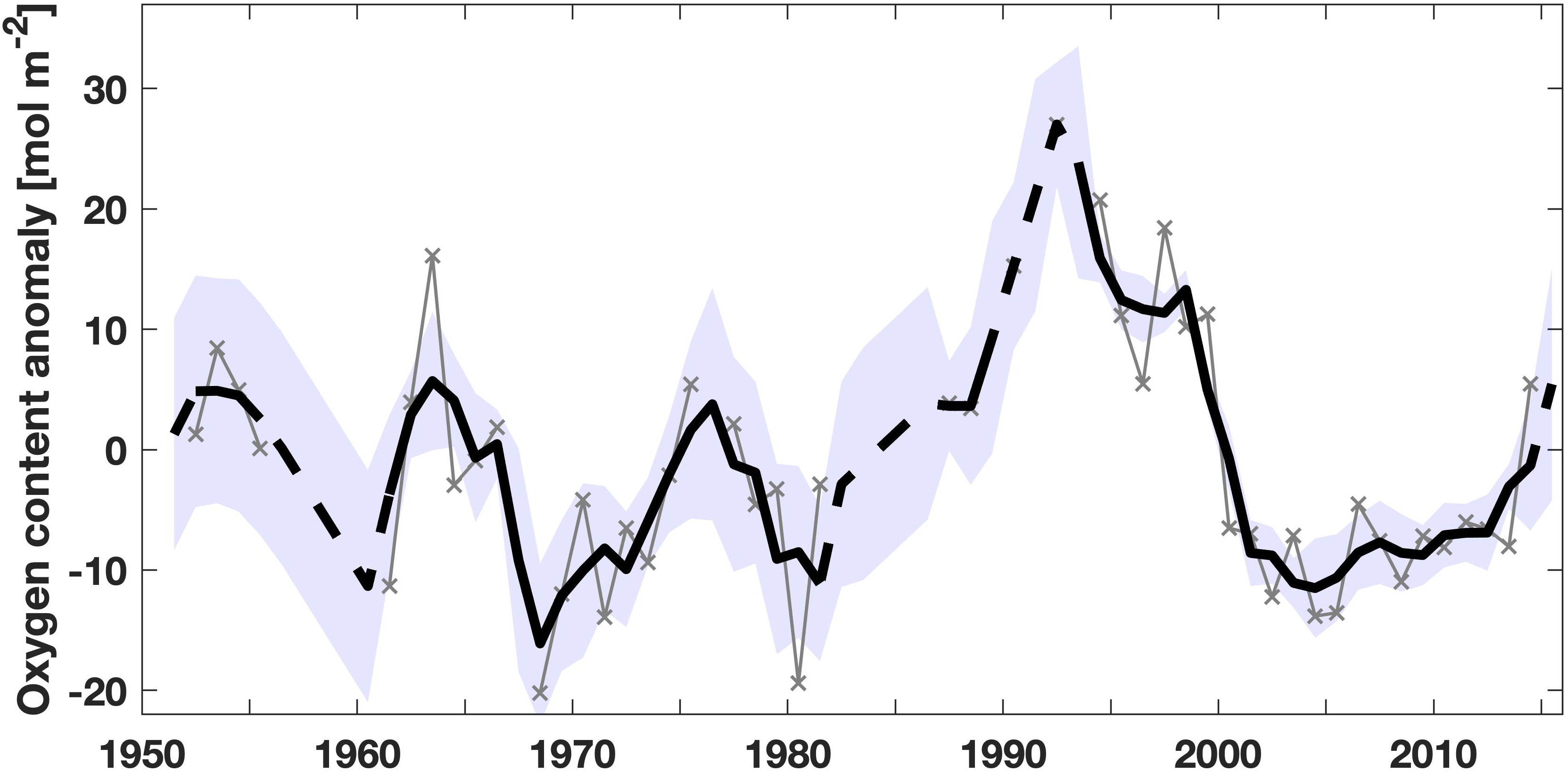
Figure 2 Time series of oxygen inventory anomaly from WOD data. Thin gray lines and symbols show annual values. The thick black line shows the time series smoothed with a 3-year running mean, and is dashed where gaps were filled. Blue shading represents the estimated error.

Although the inventory change could intuitively be assumed to be linked to gas exchange, the relationship between the two is not necessarily strictly proportional. An analysis of oxygen inventories from Argo floats showed that even during times of strong convection and larger than usual gas exchange, there is little year-to-year change in the oxygen inventory (Wolf et al., 2018). Indeed, the total increase in oxygen content over a 12-year period discussed above is only 1.5 times the uptake from the atmosphere for one single year of 22.1 mol m^–2 observed by Atamanchuk et al. (2020). Estimating the effect of eddies such as Irminger Rings advecting lower oxygen water into the central Labrador Sea, (Wolf et al., 2018) found that they could account for oxygen losses between 3.98 mol m^–2 and 11.34 mol m^–2 per year. Koelling et al. (2022) showed that about 50% of the oxygen taken up in 2017 is rapidly exported southward into the Deep Western Boundary Current, and hypothesized that additional oxygen export is associated with different pathways of LSW spreading, such as an interior flow towards the Irminger Sea that has been observed in transient tracer studies (Sy et al., 1997) and hydrographic data (Talley and McCartney, 1982; Yashayaev, 2007). Together with our time series, these results suggest that to first order, the annual net oxygen uptake from the atmosphere is largely balanced by the export of newly ventilated water out of the formation region, and its replacement with lower oxygen water from the surrounding regions, and the variability evident in Figure 2 represents the cumulative effect of the small annual residual between these two processes. The continuous loss of oxygen through outflowing LSW and its replacement with lower-oxygen water may in fact be crucial for maintaining the Labrador Sea as a net oxygen sink year after year, as it ensures that the wintertime mixed layer is far from equilibrium with the atmosphere even during years of weaker convection (Wolf et al., 2018).

3.2 The Labrador Sea’s oxygen reservoir

Given the dominant balance between gas exchange and export in the annual oxygen budget, we conclude that the oxygen content increase from 1980–1992, and decrease from 1994–2006, is a result of uptake from the atmosphere exceeding the losses from oxygen export during the former period, and export exceeding uptake during the latter. The first of these periods, referred to in the following as Period 1, encompasses the deepest reaching convection on record, which resulted in the coldest, freshest, and most oxygenated class of LSW ever observed (Yashayaev, 2007; van Aken et al., 2011). Following the peak of this convective activity in the early 1990s, the Labrador Sea experienced a period of weaker than usual convection during 1994–2006 coinciding with the decrease in oxygen content, which we will refer to as Period 2.

This time scale of the buildup and subsequent drainage of the oxygen reservoir may be related to the ocean’s “memory” in the region, which is a feature that has been observed in the Labrador Sea Water’s physical properties (Straneo et al., 2003; Yashayaev, 2007). Although there is a significant export of LSW every year (Yashayaev and Loder, 2016), some of the newly formed deep water remains in the formation region, so that the changes set by air-sea forcing during one convective season have an effect on the initial conditions during the following winter. The result is a preconditioning of the water column, making it easier for convection to penetrate deeper in a year following deep-reaching convection, and more difficult following shallower convection (Yashayaev and Loder, 2017). This process contributes to the LSW reservoir in the interior of the basin becoming progressively colder, fresher, and more oxygenated during prolonged periods of increasingly deep reaching convection (van Aken et al., 2011). At the same time, there is a continuous exchange between the interior convection region and the warmer, saltier boundary current, as well as exchanges in the inner subpolar gyre (Straneo, 2006; Yashayaev, 2007). This results in a positive advective heat flux (Yashayaev and Loder, 2009), which acts to increase stratification in the central Labrador Sea and erode the pool of homogenized deep water (Tagklis et al., 2020). This exchange, much of which happens along density surfaces, is also the main mechanism by which LSW from the interior is added to the outflowing boundary current (Georgiou et al., 2021; Zou et al., 2020). Interannual variability in the lateral exchange between the boundary current and interior Labrador Sea is related to the boundary-interior gradient of layer thickness, and the resulting advective heat gain is mostly controlled by the temperature of LSW (Straneo, 2006).

This variability in boundary-interior exchange could also affect the oxygen budget, as heat content and oxygen inventory between 0–2200 m in the central Labrador Sea are highly correlated (R = -0.83; not shown). This exchange may explain the leveling off and reversal of the inventory changes evident in Figure 2: If the exchange of oxygen, like heat, is proportional to its reservoir in the interior, a continuous increase in oxygen content would lead to an increase in the oxygen lost through exchanges with the boundary current. Eventually the export of oxygen would exceed gas exchange, with the uptake from the atmosphere no longer sufficient to replenish the oxygen that is exported out of the region, resulting in a decrease in oxygen content. This could occur either due to the continued intensification of the lateral oxygen exchange, or a decrease in oxygen uptake from the atmosphere. Since some LSW can stay in the formation region for several years (Straneo et al., 2003), the elevated oxygen export would persist for some time even after gas exchange weakened. The buildup of oxygen during Period 1, and following decrease during Period 2, would be consistent with this mechanism. During Period 1, several consecutive years of deep-reaching convection and intense oxygen uptake could explain the continued increase in oxygen content, which in turn would drive an increased boundary-interior oxygen exchange. In Period 2, the exchange would remain elevated even once the oxygen uptake weakened following peak convection, thus slowly draining the excess oxygen accumulated during Period 1.

However, from the oxygen content time series alone it is not possible to know for certain whether the mechanism proposed above is at play in the Labrador Sea. The variability could also be explained by changes in gas exchange with constant export, changes in export with constant gas exchange, or some other variability in the gas exchange-export balance that does not follow the pattern outlined above. In order to fully disentangle the relationship between decadal variability in oxygen uptake, gas exchange, and inventory change, sustained long-term observations of all three would be needed. While this may be possible in the future using the much broader coverage of in situ measurements in recent years (von Oppeln-Bronikowski et al., 2021; Atamanchuk et al., 2022; Sharp et al., 2023), at present a multi-decade observational record only exists for the oxygen inventory. In the meantime, data from ocean climate models may be a useful tool to better understand these processes, which is the focus of the following section.

4 Oxygen budget in CMIP6-OMIP1

In this section, we use data from nine different CMIP6 models in order to analyze the balance between the different terms in the oxygen budget. We use output from all models that participated in the OMIP1 phase and provided fields of oxygen and air-sea flux of oxygen, as described in section 2. Section 4.1 focuses on evaluating how well the models reproduce the observational record, and uses the score defined in Section 2.4 to assess model performance. In section 4.2, we use the ensemble mean in order to diagnose differences in gas exchange, oxygen export, and oxygen storage between the two periods defined in section 3.2.

4.1 Model evaluation

Figure 3A shows the central Labrador Sea’s oxygen inventory anomaly between 0-2200 m taken from nine different CMIP6-OMIP1 models that include ocean biogeochemistry, as well as the mean of all models (see Section 2 for details). While there is some spread between the modeled oxygen inventory in any given year, they all exhibit variability similar to observations on decadal time scales. In particular, a maximum in oxygen content in the mid-1990s is evident in all models, suggesting that the impact of the record-deep convection during this time (Yashayaev, 2007) is reproduced to some extent in CMIP6-OMIP1. However, the magnitude of the peak oxygen content anomaly is reduced by about half compared to the observational record.

FIGURE 3

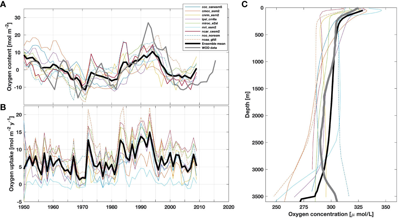
Figure 3 Comparison of CMIP6-OMIP1 model data from the central Labrador Sea to observations. In all panels, the thick black line shows the mean of all models, and in panels (A) and (C) the grey line shows the observational data from WOD. (A) Oxygen content anomaly (B) Annual mean air-sea gas exchange of oxygen (C) Mean profiles of oxygen concentration.

A possible explanation for this discrepancy could be the representation of gas exchange in climate models. The biogeochemical protocols for participants of OMIP (Orr et al., 2017) state that modelers should use the gas exchange parameterization of Wanninkhof (1992) with the updated coefficients of Wanninkhof, 2014. This parameterization is constrained to reproduce global air-sea fluxes of carbon, but has been shown to substantially underestimate oxygen uptake in the Labrador Sea because it does not include a bubble-mediated term, which makes up a significant fraction of the total gas exchange for oxygen in this region (Koelling et al., 2017; Atamanchuk et al., 2020). Figure 3B shows the time series of the annual gas exchange from the CMIP6-OMIP1 models, with time-mean values provided in Table S1. Indeed, the models seem to significantly underestimate the gas exchange observed in the real ocean: The highest mean annual gas exchange from any of the models is 10.91 mol m^–2 (NOAA GFDL), which is less than half of the uptake inferred by Atamanchuk et al. (2020) and Wolf et al. (2018), but comparable to an early estimate by Körtzinger et al. (2008) that used the Wanninkhof (1992) parameterization. The mean annual gas exchange for the ensemble mean is 7.22 mol m^–2, about a third of observation-based estimates. This strong discrepancy with the observed data highlights again the need for critical evaluation of gas exchange parameterizations for oxygen in climate models as called for in previous studies (Atamanchuk et al., 2020; Seltzer et al., 2023).

Another issue common in CMIP is that modelled convection depths in the Labrador Sea are often much deeper than in observations (Heuzé, 2017; Heuzé, 2021), which may be related to their inability to resolve submesoscale processes (Tagklis et al., 2020). As a result, Labrador Sea Water in these models penetrates deeper than observed in the real ocean, and the deep overflow water masses below LSW are much less pronounced than in observations. This is evident in Figure 3C, as neither the low-oxygen Northeast Atlantic Deep Water (NEADW) layer from about 1500–3000 m depth, nor the near-bottom oxygen maximum associated with Denmark Strait Overflow Water (Yashayaev and Loder, 2017), are discernible in the model mean oxygen profile. The effect of unrealistically deep-reaching convection can also be seen in oxygen concentration anomalies (Figure 4). In particular, the IPSL CM6a, MRI ESM2, and NOAA GFDL models have the maximum anomalies in oxygen concentrations near the bottom, rather than in the 1000–2000 m depth range typically occupied by LSW in the real ocean, and all three of these models have been shown to have much deeper convection compared to observations (Adcroft et al., 2019; Boucher et al., 2020; Jackson and Petit, 2022). This is another factor that can contribute to the underestimation of oxygen content anomalies in the LSW layer (Figure 3A), as the variability in LSW oxygen in these models is spread over the whole water column, rather than just 0–2200 m. The lack of realistic overflow water masses could also be contributing to gas exchange being too weak. During some years, convection can penetrate into the salty, low-oxygen NEADW layer underlying LSW, incorporating it into the newly formed water mass (Yashayaev, 2007). This entrainment of old waters with lower oxygen is an important driver for maintaining undersaturation of surface waters throughout the convective season (Wolf et al., 2018). Thus, the lack of a clear oxygen minimum below LSW (Figure 3C) could result in surface oxygen concentrations being too close to saturation, reducing the magnitude of the calculated oxygen uptake.

FIGURE 4

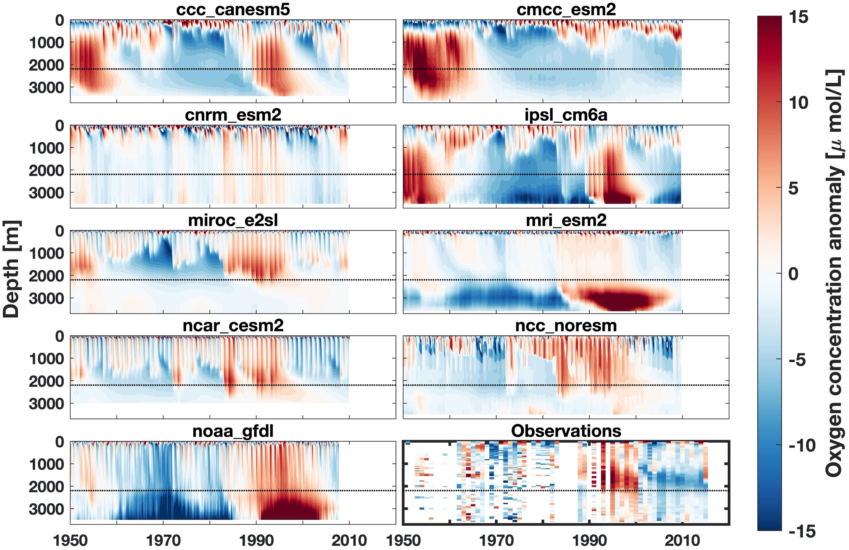
Figure 4 Oxygen concentration anomaly contour plots for all CMIP6-OMIP1 models used, and the observational estimate. Anomalies are calculated relative to the mean at each depth level. The thin dashed line in each panel is at 2200 m, the integration depth for the oxygen inventory time series.

Overall, while there generally is decadal variability in oxygen content at similar time scales to observations, many CMIP6-OMIP1 models seem to struggle with representing the more detailed aspects of the Labrador Sea’s oxygen dynamics. This includes weaker amplitude of the decadal signal (Figure 3A), reduced mean oxygen uptake (Figure 3B), biases in the mean oxygen profile (Figure 3C), and excessively deep convection (Figure 4). In order to assess each model’s performance in these areas, we calculated a score based on five factors, as described in section 2.4, and the scores for each metric as well as the total score are given in Table 2.

TABLE 2

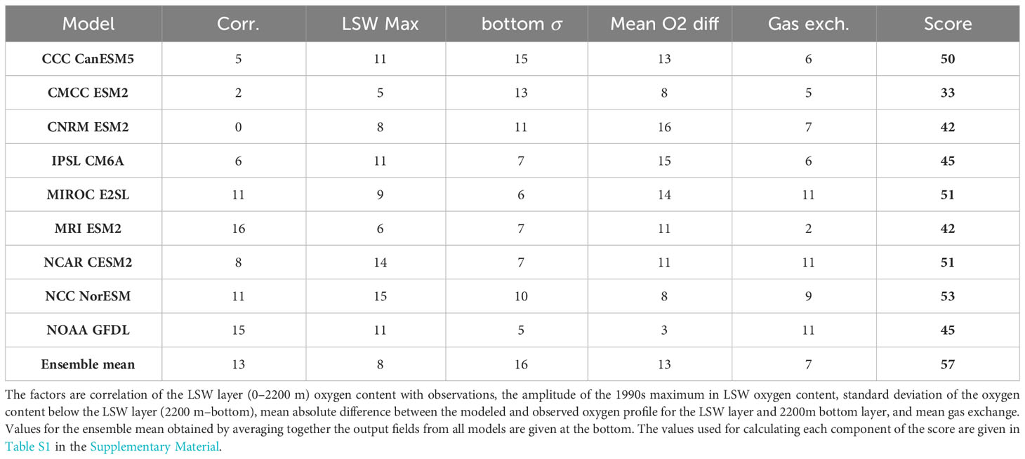
Table 2 Scores for each of the five components used in constructing the model score, and total score for each model.

The majority of the models score close to 50 out of 100 points, and none higher than 53/100. Based on the different score components (Table 2) the exact nature of the mismatch with observations is different for each model. For example, MRI ESM2 scores the highest on the correlation with the LSW time series, but also has a low amplitude for the LSW maximum, too much variability below the LSW layer, and the weakest mean gas exchange. Conversely, the NCAR CESM2 model does well for the amplitude of the maximum and the mean gas exchange, but the correlation with the observational time series is weaker. Using the ensemble mean of all models results in a better score than any individual model, consistent with the expectation that the mean of an ensemble of models generally is closer to the “true” signal than individual members (Collins et al., 2014). However, even the ensemble mean only achieves a score of 57, with shortcomings evident particularly in the amplitude of the oxygen inventory maximum and the mean gas exchange.

While the exact scores are somewhat arbitrary, these results highlight the need for improvements in modelling the oxygen cycle in this key region for deep ocean ventilation. Given that models are our only tool for projections of future ocean deoxygenation, we echo Oschlies et al. (2018)’s sentiment that discrepancies between models and observations need to be resolved in order to understand how oxygen levels may change in the future. We hope that the model score created here can contribute to that cause, providing an easy and consistent way to evaluate how key metrics related to deep ocean ventilation in the Labrador Sea are represented in ocean models.

4.2 Balance between oxygen storage, gas exchange, and export

Despite the CMIP6-OMIP1 model’s shortcomings discussed above, they can be useful for testing the links between gas exchange, oxygen content change, and export in the Labrador Sea. In particular, the increase in the oxygen inventory associated with the 1987-1994 class of LSW in Period 1, and subsequent decrease in Period 2, is present in all models (Figure 3A), albeit with reduced magnitude. Below, we assess how the different terms of the oxygen budget in the Labrador Sea vary during this record deep convection period in the CMIP6-OMIP1 models.

To test how the decadal oxygen content variability is controlled by gas exchange and oxygen export, we calculate annual oxygen storage rates and gas exchange using the ensemble mean of the nine CMIP6-OMIP1 models, and infer the export as the residual by rearranging equation 1. Figure 5A shows the time series of the annual mean gas exchange and oxygen storage from the model outputs. Oxygen storage is the year-to-year change in the oxygen inventory, i.e. the first derivative of the time series shown in Figure 3A. The long-term mean is 7.22 mol m^–2 y^–1 for the gas exchange and 0 mol m^–2 y^–1 for the storage term. Thus, the mean of the export, calculated as the residual, is also 7.22 mol m^–2 y^–1: On long time scales, the net annual oxygen uptake is balanced by a net export of oxygen. Interannual variability in gas exchange is positively correlated with variability in storage (R = 0.66 for the multi-model mean, Figure 5B) as well as export (R = 0.64, Figure 5C), while there is relatively little correlation between export and storage (R = -0.11, not shown). This suggests that both storage and export are driven mostly by variability in oxygen uptake, with both the local oxygen inventory and the amount of oxygen that is exported increasing during years with more intense air-sea gas exchange, and decreasing when less oxygen is taken up. There is also a relationship between the oxygen content anomaly (Figure 3A) and oxygen export, with a correlation of R = 0.73. This would be consistent with a lateral exchange of oxygen that is proportional to the boundary-interior gradient, as proposed in section 3.2.

FIGURE 5

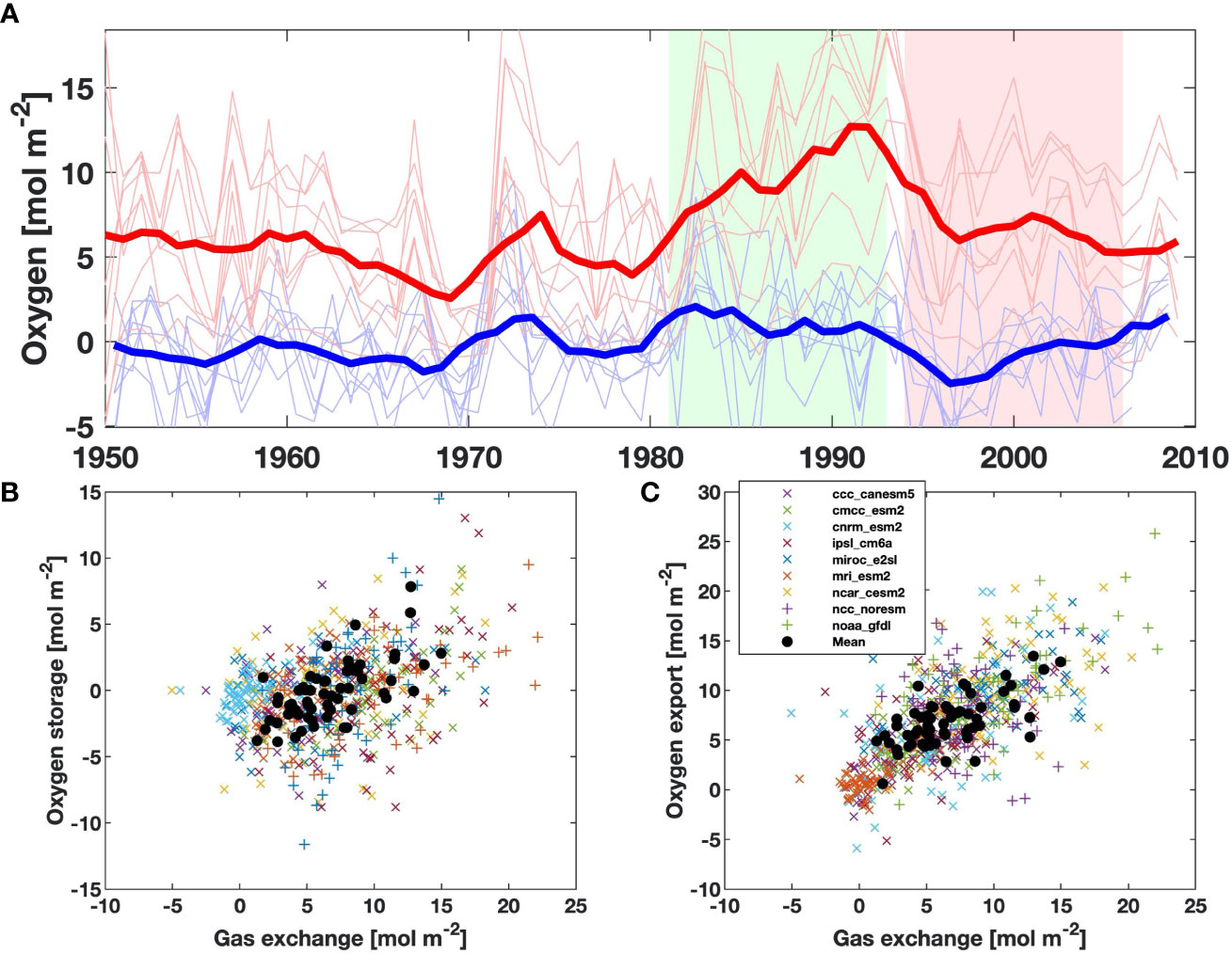
Figure 5 (A) Time series of annual gas exchange (red) and oxygen storage (blue) from the CMIP6-OMIP1 models used in this study. Thin lines show individual models, and thick lines show the ensemble mean, smoothed with a 5-year running mean filter. Mean values for the two periods are given in Table 3. (B) Relationship between annual gas exchange and oxygen storage (C) Relationship between annual gas exchange and export. In panels (B, C), individual models are shown as colored symbols, and black circles show the multi-model mean.

On decadal time scales, variability in oxygen storage can be an important factor in controlling the linkage between uptake and export. Period 1 and 2 are shaded in Figure 5A in green and red, respectively, and mean values of the three terms over each period are shown in Table 3, with the values for individual models summarized in Table S2. By definition, the storage term is generally positive in the first period (1.07 mol m^–2 y^–1) and negative in the latter (-1.22 mol m^–2 y^–1), although there is also interannual and inter-model variability around this mean. The period of positive storage changes is accompanied by the largest gas exchange over the model record (9.60 mol m^–2 y^–1), while oxygen uptake during the second period is 6.89 $mol{m}^{-2}{y}^{-1}$, slightly less than the long-term average. The difference in gas exchange exceeds the difference in oxygen storage because the oxygen export is also stronger in Period 1 than Period 2, changing from 8.52 $mol{m}^{-2}{y}^{-1}$ to 8.11 mol m^–2 y^–1. The modelled data suggest that the period of record strong convection in the 1980s and early 1990s featured the record strongest gas exchange and oxygen storage (Figure 5A), as well as the record oxygen export (not shown).

TABLE 3

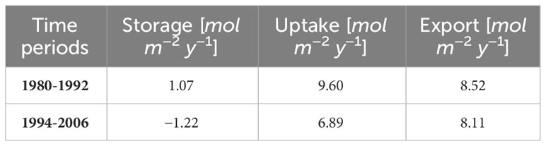
Table 3 Terms of the oxygen budget (eq. 1) in CMIP6-OMIP1 models for Period 1 and Period 2.

Although both oxygen uptake and oxygen export are decreased in Period 2 compared to their record values in Period 1, the change in the latter is much smaller: A 2.71 mol m^–2 y^–1 change in gas exchange only corresponds to a change in oxygen export by 0.40 mol m^–2 y^–1, or 14% of the decreased uptake. The remainder is balanced by a decrease in oxygen storage of 2.29 mol m^–2 y^–1, 85% of oxygen uptake change, as the oxygen reservoir switches from accumulating excess oxygen to exporting more than is added. This suggests that although the dominant balance in the long-term mean is between gas exchange and export, oxygen storage in the interior Labrador Sea can be important for modulating their variability on decadal time scales, acting as a buffer between increased uptake and increased export. The switch between the two periods from positive to negative oxygen storage, and stronger to weaker gas exchange, are robust across all models (Table S2). The change in export is negative in most models, but there is a wider range of behaviors, likely reflecting differences in model physics such as ocean circulation.

Our analysis of the CMIP6-OMIP1 data thus suggests that although much of the oxygen taken up from the atmosphere is exported out of the formation region, there is also an accumulation, or storage, of oxygen in the interior Labrador Sea during periods of high oxygen uptake, consistent with a multi-year residence time of LSW (Straneo et al., 2003). This oxygen storage acts as a buffer, partially decoupling the export of oxygen out of the region from the uptake via gas exchange, dampening the impact of variations in oxygen uptake on export, and ensuring a more steady deep water oxygen supply to the rest of the ocean.

5 Implications

5.1 Ventilation and deoxygenation in CMIP6-OMIP1

Our analysis shows that contemporary CMIP6-OMIP1 models struggle to accurately portray the magnitude of oxygen content changes, the mean vertical profile of oxygen, and mean air-sea gas exchange in the Labrador Sea (section 4.1, Table 2), suggesting a need for improvement of modeled oxygen cycles in this region.

This is particularly true given the importance of the Labrador Sea and the subpolar North Atlantic as a whole for ventilating the global ocean. A major shortcoming appears to be the representation of air-sea gas exchange, with CMIP6-OMIP1 models estimating the annual net oxygen uptake to be only about a third of observed values. This is in line with previous studies in the region that had shown the gas exchange parameterization used in CMIP6-OMIP1 models to severely underestimate oxygen uptake during deep convection in winter (Koelling et al., 2017; Atamanchuk et al., 2020; Seltzer et al., 2023), and could be responsible for the reduced magnitude of oxygen content changes compared to observations. Another contributing factor may be the difficulties that some CMIP6-OMIP1 models have with modelling convection to realistic depths (Figure 4) and representing overflow water masses (Figure 3C), which can lead to biases in oxygen distributions throughout the water column, including surface oxygen being too close to saturation during deep convection.

Since gas exchange is balanced primarily by oxygen export out of the region this weaker oxygen uptake would also result in too little supply of oxygen from the deep water formation area to the rest of the global ocean in CMIP6-OMIP1 models. Given that the bubble-mediated gas flux is important for air-sea gas exchange in the other major deep ocean ventilation region, the Southern Ocean (Bushinsky et al., 2017), it may be expected that oxygen uptake, storage, and export there are likewise underestimated. Consequently, the mean strength of deep ocean ventilation in both subpolar regions as currently represented in global climate models, as well its variability, may be too small. This would be consistent with a recent finding that climate models underestimate ventilation changes (Buchanan and Tagliabue, 2021), and could partially explain discrepancies in ocean deoxygenation between models and observations (Oschlies et al., 2017; Oschlies et al., 2018). Furthermore, if the oxygen supply to the deep ocean is underestimated in global climate models, then its consumption by marine organisms would have to also be too weak in order to avoid spurious trends in global oxygen concentrations in the interior ocean. This might have important implications not only for future ocean deoxygenation, but also for model-based studies of the biological carbon pump (BCP), as too little oxygen consumption would correspond to too little carbon remineralization in the deep ocean. An improved representation of deep ocean ventilation with oxygen therefore seems imperative for predicting the evolution of both deoxygenation and the BCP in a changing ocean.

5.2 Gas exchange and oxygen export

Despite shortcomings, one aspect that the CMIP6-OMIP1 models do reproduce fairly consistently in the Labrador Sea is the interannual and decadal variability of the oxygen content. Although the magnitude is too weak, the correlation of the time series with the observational dataset is 0.73 for the ensemble mean (Table S1), and all models show positive oxygen storage from 1980 to 1992, and negative storage from 1994 to 2006 (Table S2). Given that the oxygen content change is related to variability in air-sea gas exchange (Section 4.2), this may suggest that although the magnitude of the gas exchange is too low in the models, its temporal variability (Figure 3B) more accurately reproduces that of the real ocean.

The mean balance in the oxygen budget in both observations and models is largely between gas exchange and export: There is almost no long-term change in storage over the 60-year period that was analyzed (sections 3.1, 4.2), meaning that the average amount of oxygen exported is equivalent to the average amount taken up from the atmosphere. However, much of the decadal variability in gas exchange seen in the CMIP6-OMIP1 models is imprinted onto the oxygen content, rather than the export. Between the strong convection period 1980–1992 and the weak convection period 1994–2006, the mean annual gas exchange decreases by 2.71 mol m^–2 (28% change from Period 1 mean) in CMIP6-OMIP1 models, 85% of which is balanced by the change in the annual storage rate (2.29 mol m^–2), while only 14% of the decreased gas exchange is reflected in the oxygen export (0.40 mol m^–2, 5% of Period 1 mean). Thus, while the interannual to decadal variability in oxygen uptake does affect the export, its magnitude is dampened by the accumulation and subsequent drainage of oxygen in the central Labrador Sea. [Körtzinger et al. (2004)] using one of the first deployments of biogoeochemical Argo floats, referred to the wintertime oxygen uptake in the Labrador Sea as the ocean “taking a deep breath”. Our results show that the multi-year residence time of LSW in the interior of the basin leads to the ocean “holding its breath”, storing some of the excess oxygen taken up during strong convection years, and exporting it in subsequent years.

This relative insensitivity of the export to atmospheric forcing reported here differs from estimates based on the change in layer thickness of LSW, which suggest almost a factor of 3 difference in the volume of LSW export between strong and weak convection years (Yashayaev and Loder, 2016). The difference may stem from the fact that their analysis highlights the export of LSW over a 1-year period following the previous convection season, while the oxygen-based estimate discussed here includes the export of older LSW as well. During particularly strong convection periods, stronger gas exchange does lead to increased export, but also increases the oxygen content in the formation region since some of the newly formed LSW stays in the region from one year to the next (Straneo et al., 2003). This “storage” affects the export in subsequent years, such that some of the LSW and oxygen export from a strong convection period continues even after convection has weakened and the oxygen uptake has decreased.

On the other hand, if convection in the Labrador Sea were to continuously weaken or stop altogether as a result of climate change, as has been suggested could occur [e.g. (Oltmanns et al. (2018)], the oxygen uptake, and therefore also the export, would likely decrease dramatically. The shallower mixed layer would reach equilibrium quickly, limiting the amount of oxygen that can be taken up, while the absence of convection would also impede any supply of this atmospheric oxygen to the deep ocean. Due to the time lag between oxygen uptake and export introduced by the Labrador Sea’s oxygen reservoir, there would still be a net flow of oxygen out of the basin for some time, but its rate would continuously decrease as the oxygen stored in the interior Labrador Sea slowly drains out along LSW export pathways. Eventually, the deep oxygen reservoir would disappear, and the Labrador Sea would no longer act as a source of oxygen for the deep ocean, with potentially grave impacts for marine ecosystems as the ocean loses its breath.

One key question that remains is how uptake and export of oxygen in the Labrador Sea are related to the strength of the Atlantic Meridional Oveturning Circulation (AMOC). The strength of the AMOC varies on decadal time scales (Moat et al., 2020; Jackson et al., 2022; Le Bras et al., 2023), and future projections with CMIP models suggest that it will weaken over the next century (Bakker et al., 2016; Weijer et al., 2020). In the Labrador Sea, this would mean a decreased strength of both the outflowing boundary current, which is responsible for some of the oxygen export (Koelling et al., 2022), and the flow of lower-oxygen water into the basin. In an analysis of decadal changes in oxygen concentrations in the neighboring Irminger Sea, Feucher et al. (2022) found that changes in ocean circulation play an important role in controlling oxygen variability. In contrast, our analysis of CMIP6-OMIP1 output suggests that the oxygen export does not play a major role for the oxygen content in the interior Labrador Sea, with most of the variability in both oxygen content and export set by changes in the uptake from the atmosphere. However, while this is true for the multi-model mean, individual models do have a larger correlation between oxygen storage and export, suggesting that this finding is dependent on model physics. A more detailed analysis of the differences in circulation between the models is beyond the scope of the current study, but could provide further insight into whether there is a linkage between the AMOC and oxygen transports. Our understanding of these processes will also benefit from the addition of oxygen sensors to the OSNAP mooring array, which will enable calculation of cross-basin oxygen transports associated with the overturning circulation (Atamanchuk et al., 2022).

In order to be able to monitor and predict the future variability in ventilation in this basin and the subpolar North Atlantic as a whole, the long-term context provided by the present study will need to be combined with more detailed analyses of the present-day oxygen uptake and export on basin-wide scales. In recent years, there have been regular oxygen measurements from gliders in the Labrador Sea (von Oppeln-Bronikowski et al., 2021), the use of moored oxygen sensors in the SPNA has increased dramatically (Atamanchuk et al., 2022), and with the proliferation of BGC-Argo floats throughout the ocean, full global 4-D fields of oxygen based on observational data are now becoming available (Sharp et al., 2023). This wealth of data concentrated in a small but key area of the ocean could be exploited in the future to study ocean ventilation by constraining the uptake, storage, and export of oxygen in much more detail than was possible in the present study, and guide improvement in how these processes are implemented in climate models. Given our current lack of knowledge about the mechanisms driving deoxygenation and changes in deep ocean ventilation (Oschlies et al., 2018), improving our understanding of these topics, and their representation in models, will be imperative for reliably predicting how they may change in the future.

Data availability statement

Publicly available datasets were analyzed in this study. This data can be found here: https://esgf-node.llnl.gov/search/cmip6/; https://www.ncei.noaa.gov/products/world-ocean-database.

Author contributions

Data analysis for this study was carried out by JKo. The manuscript was prepared by JKo, with contributions from all other coauthors. All authors contributed to the article and approved the submitted version.

Funding

JKo was funded in part by the Ocean Frontier Institute through the International Postdoctoral Fellowship. This work was funded in part by the Canada Excellence Research Chair in Ocean Science and Technology. The research was also supported by funding from the Canada First Research Excellence Fund, through the Ocean Frontier Institute, module B: “Auditing the Northwest Atlantic Carbon Sink”.

Acknowledgments

We acknowledge the World Climate Research Programme, which, through its Working Group on Coupled Modelling, coordinated and promoted CMIP6. We thank the climate modeling groups for producing and making available their model output, the Earth System Grid Federation (ESGF) for archiving the data and providing access, and the multiple funding agencies who support CMIP6 and ESGF. We would like to thank the reviewers for useful criticisms and suggestions which focused and improved the manuscript.

Conflict of interest

The authors declare that the research was conducted in the absence of any commercial or financial relationships that could be construed as a potential conflict of interest.

Publisher’s note

All claims expressed in this article are solely those of the authors and do not necessarily represent those of their affiliated organizations, or those of the publisher, the editors and the reviewers. Any product that may be evaluated in this article, or claim that may be made by its manufacturer, is not guaranteed or endorsed by the publisher.

Supplementary material

The Supplementary Material for this article can be found online at: https://www.frontiersin.org/articles/10.3389/fmars.2023.1202299/full#supplementary-material

References

Adcroft A., Anderson W., Balaji V., Blanton C., Bushuk M., Dufour C. O., et al. (2019). The gfdl global ocean and sea ice model om4.0: Model description and simulation features. J. Adv. Modeling Earth Syst. 11, 3167–3211. doi: 10.1029/2019MS001726

CrossRef Full Text | Google Scholar

Anav A., Friedlingstein P., Kidston M., Bopp L., Ciais P., Cox P., et al. (2013). Evaluating the land and ocean components of the global carbon cycle in the CMIP5 earth system models. J. Climate 26, 6801–6843. doi: 10.1175/JCLI-D-12-00417.1

CrossRef Full Text | Google Scholar

Atamanchuk D., Koelling J., Send U., Wallace D. (2020). Rapid transfer of oxygen to the deep ocean mediated by bubbles. Nat. Geosci. 13 (3), 232–237. doi: 10.1038/s41561-020-0532-2

CrossRef Full Text | Google Scholar

Atamanchuk D., Palter J., Palevsky H., Le Bras I., Koelling J., Nicholson D. (2022). “Linking Oxygen and Carbon Uptake with the Meridional Overturning Circulation using a Transport Mooring Array,” in Frontiers in ocean Observing: Documenting Ecosystems, Understanding Environmental Changes, Forecasting Hazards. Eds. Kappel E., Juniper S., Seeyave S., Smith E., Visbeck M., 9. doi: 10.5670/oceanog.2021.supplement.02-03

CrossRef Full Text | Google Scholar

Bakker P., Schmittner A., Lenaerts J. T. M., Abe-Ouchi A., Bi D., van den Broeke M. R., et al. (2016). Fate of the Atlantic Meridional Overturning Circulation: Strong decline under continued warming and Greenland melting. Geophysical Res. Lett. 43, 12,252–12,260. doi: 10.1002/2016GL070457

CrossRef Full Text | Google Scholar

Boucher O., Servonnat J., Albright A. L., Aumont O., Balkanski Y., Bastrikov V., et al. (2020). Presentation and evaluation of the ipsl-cm6a-lr climate model. J. Adv. Modeling Earth Syst. 12, e2019MS002010. doi: 10.1029/2019MS002010

CrossRef Full Text | Google Scholar

Boyer T. P., Antonov J. I., Baranova O. K., Coleman C., Garcia H. E., Grodsky A., et al. (2013). World ocean database 2013. doi: 10.7289/V5NZ85MT

CrossRef Full Text | Google Scholar

Buchanan P. J., Tagliabue A. (2021). The regional importance of oxygen demand and supply for historical ocean oxygen trends. Geophysical Res. Lett. 48, e2021GL094797. doi: 10.1029/2021GL094797

CrossRef Full Text | Google Scholar

Bushinsky S. M., Gray A. R., Johnson K. S., Sarmiento J. L. (2017). Oxygen in the southern ocean from argo floats: determination of processes driving air-sea fluxes. J. Geophysical Research: Oceans 122, 8661–8682. doi: 10.1002/2017JC012923

CrossRef Full Text | Google Scholar

Collins M., Knutti R., Arblaster J., Dufresne J.-L., Fichefet T., Friedlingstein P., et al. (2014). “Long-term Climate Change: Projections, Commitments and Irreversibility,” in Climate Change 2013 – The Physical Science Basis: Working Group I Contribution to the Fifth Assessment Report of the Intergovernmental Panel on Climate Change (Cambridge: Cambridge University Press), 1029–1136. doi: 10.1017/CBO9781107415324.024

CrossRef Full Text | Google Scholar

Feucher C., Portela E., Kolodziejczyk N., Thierry V. (2022). Subpolar gyre decadal variability explains the recent oxygenation in the Irminger Sea. Commun. Earth Environ. 3, 279. doi: 10.1038/s43247-022-00570-y

CrossRef Full Text | Google Scholar

Georgiou S., Ypma S. L., Brüggemann N., Sayol J.-M., van der Boog C. G., Spence P., et al. (2021). Direct and indirect pathways of convected water masses and their impacts on the overturning dynamics of the Labrador Sea. J. Geophysical Research: Oceans 126 (1), e2020JC016654. doi: 10.1029/2020JC016654

CrossRef Full Text | Google Scholar

Gleckler P. J., Taylor K. E., Doutriaux C. (2008). Performance metrics for climate models. J. Geophysical Research: Atmospheres 113. doi: 10.1029/2007JD008972

CrossRef Full Text | Google Scholar

Heuzé C. (2017). North Atlantic deep water formation and AMOC in CMIP5 models. Ocean Sci. 13, 609–622. doi: 10.5194/os-13-609-2017

CrossRef Full Text | Google Scholar

Heuzé C. (2021). Antarctic bottom water and north atlantic deep water in CMIP6 models. Ocean Sci. 17, 59–90. doi: 10.5194/os-17-59-2021

CrossRef Full Text | Google Scholar

Huang J., Huang J., Liu X., Li C., Ding L., Yu H. (2018). The global oxygen budget and its future projection. Sci. Bull. 63, 1180–1186. doi: 10.1016/j.scib.2018.07.023

CrossRef Full Text | Google Scholar

Ito T., Minobe S., Long M. C., Deutsch C. (2017). Upper ocean O2 trends: 1958–2015. Geophysical Res. Lett. 44, 4214–4223. doi: 10.1002/2017GL073613

CrossRef Full Text | Google Scholar

Jackson L. C., Biastoch A., Buckley M. W., Desbruyerès D. G., Frajka-Williams E., Moat B., et al. (2022). The evolution of the North Atlantic meridional overturning circulation since 1980. Nat. Rev. Earth Environ. 3, 241–254. doi: 10.1038/s43017-022-00263-2

CrossRef Full Text | Google Scholar

Jackson L., Petit T. (2022). North Atlantic overturning and water mass transformation in CMIP6 models. Climate Dynamics 60 (9-10), 1–21. doi: 10.1007/s00382-022-06448-1

CrossRef Full Text | Google Scholar

Karstensen J., Stramma L., Visbeck M. (2008). Oxygen minimum zones in the eastern tropical Atlantic and Pacific oceans. Prog. Oceanography 77, 331–350. doi: 10.1016/j.pocean.2007.05.009

CrossRef Full Text | Google Scholar

Kieke D., Yashayaev I. (2015). Studies of Labrador Sea Water formation and variability in the subpolar North Atlantic in the light of international partnership and collaboration. Prog. Oceanography 132, 220–232. doi: 10.1016/j.pocean.2014.12.010

CrossRef Full Text | Google Scholar

Koelling J., Atamanchuk D., Karstensen J., Handmann P., Wallace D. W. R. (2022). Oxygen export to the deep ocean following Labrador Sea Water formation. Biogeosciences 19, 437–454. doi: 10.5194/bg-19-437-2022

CrossRef Full Text | Google Scholar

Koelling J., Wallace D. W. R., Send U., Karstensen J. (2017). Intense oceanic uptake of oxygen during 2014–2015 winter convection in the Labrador Sea. Geophysical Res. Lett. 44, 7855–7864. doi: 10.1002/2017GL073933

CrossRef Full Text | Google Scholar

Koenigk T., Fuentes-Franco R., Meccia V. L., Gutjahr O., Jackson L. C., New A. L., et al. (2021). Deep mixed ocean volume in the Labrador Sea in HighResMIP models. Climate Dynamics 57, 1895–1918. doi: 10.1007/s00382-021-05785-x

CrossRef Full Text | Google Scholar

Körtzinger A., Schimanski J., Send U., Wallace D. (2004). The ocean takes a deep breath. Science 306, 1337–1337. doi: 10.1126/science.1102557

PubMed Abstract | CrossRef Full Text | Google Scholar

Körtzinger A., Send U., Wallace D. W., Karstensen J., DeGrandpre M. (2008). Seasonal cycle of O2 and pCO2 in the central Labrador Sea: Atmospheric, biological, and physical implications. Global Biogeochemical Cycles 22. doi: 10.1029/2007GB003029

CrossRef Full Text | Google Scholar

Large W., Yeager S. (2009). The global climatology of an interannually varying air–sea flux data set. Climate dynamics 33, 341–364. doi: 10.1007/s00382-008-0441-3

CrossRef Full Text | Google Scholar

Laurent A., Fennel K., Kuhn A. (2021). An observation-based evaluation and ranking of historical Earth system model simulations in the northwest North Atlantic Ocean. Biogeosciences 18, 1803–1822. doi: 10.5194/bg-18-1803-2021

CrossRef Full Text | Google Scholar

Le Bras I. A.-A., Willis J., Fenty I. (2023). The atlantic meridional overturning circulation at 35°N from deep moorings, floats, and satellite altimeter. Geophysical Res. Lett. 50, e2022GL101931. doi: 10.1029/2022GL101931

CrossRef Full Text | Google Scholar

Martz T. R., DeGrandpre M. D., Strutton P. G., McGillis W. R., Drennan W. M. (2009). Sea surface pCO2 and carbon export during the Labrador Sea spring-summer bloom: An in situ mass balance approach. J. Geophysical Research: Oceans 114. doi: 10.1029/2008JC005060

CrossRef Full Text | Google Scholar

Moat B. I., Smeed D. A., Frajka-Williams E., Desbruyerès ,. D. G., Beaulieu C., Johns W. E., et al. (2020). Pending recovery in the strength of the meridional overturning circulation at 26N. Ocean Sci. 16, 863–874. doi: 10.5194/os-16-863-2020

CrossRef Full Text | Google Scholar

Oltmanns M., Karstensen J., Fischer J. (2018). Increased risk of a shutdown of ocean convection posed by warm North Atlantic summers. Nat. Climate Change 8, 300–304. doi: 10.1038/s41558-018-0105-1

CrossRef Full Text | Google Scholar

Orr J. C., Najjar R. G., Aumont O., Bopp L., Bullister J. L., Danabasoglu G., et al. (2017). Biogeochemical protocols and diagnostics for the CMIP6 Ocean Model Intercomparison Project (OMIP). Geoscientific Model. Dev. 10, 2169–2199. doi: 10.5194/gmd-10-2169-2017

CrossRef Full Text | Google Scholar

Oschlies A., Brandt P., Stramma L., Schmidtko S. (2018). Drivers and mechanisms of ocean deoxygenation. Nat. Geosci. 11, 467–473. doi: 10.1038/s41561-018-0152-2

CrossRef Full Text | Google Scholar

Oschlies A., Duteil O., Getzlaff J., Koeve W., Landolfi A., Schmidtko S. (2017). Patterns of deoxygenation: sensitivity to natural and anthropogenic drivers. Philos. Trans. R. Soc. A: Mathematical Phys. Eng. Sci. 375, 20160325. doi: 10.1098/rsta.2016

CrossRef Full Text | Google Scholar

Portela E., Kolodziejczyk N., Vic C., Thierry V. (2020). Physical mechanisms driving oxygen subduction in the global ocean. Geophysical Res. Lett. 47, e2020GL089040. doi: 10.1029/2020GL089040

CrossRef Full Text | Google Scholar

Rhein M., Steinfeldt R., Kieke D., Stendardo I., Yashayaev I. (2017). Ventilation variability of Labrador Sea Water and its impact on oxygen and anthropogenic carbon: a review. Philos. Trans. R. Soc. A: Mathematical Phys. Eng. Sci. 375, 20160321. doi: 10.1098/rsta.2016.0321

CrossRef Full Text | Google Scholar

Rickard G. J., Behrens E., Chiswell S. M. (2016). CMIP5 earth system models with biogeochemistry: An assessment for the southwest Pacific Ocean. J. Geophysical Research: Oceans 121, 7857–7879. doi: 10.1002/2016JC011736

CrossRef Full Text | Google Scholar

Schmidtko S., Stramma L., Visbeck M. (2017). Decline in global oceanic oxygen content during the past five decades. Nature 542, 335–339. doi: 10.1038/nature21399

PubMed Abstract | CrossRef Full Text | Google Scholar

Seltzer A. M., Nicholson D. P., Smethie W. M., Tyne R. L., Roy E. L., Stanley R. H. R., et al. (2023). Dissolved gases in the deep North Atlantic track ocean ventilation processes. Proc. Natl. Acad. Sci. 120, e2217946120. doi: 10.1073/pnas.2217946120

CrossRef Full Text | Google Scholar

Sharp J. D., Fassbender A. J., Carter B. R., Johnson G. C., Schultz C., Dunne J. P., et al. (2022). GOBAI-O2: A global gridded monthly dataset of ocean interior dissolved oxygen concentrations based on shipboard and autonomous observations (NCEI Accession 0259304 v1.1). NOAA National Centers for Environmental Information. Dataset. doi: 10.25921/z72m-yz67

CrossRef Full Text | Google Scholar

Sharp J. D., Fassbender A. J., Carter B. R., Johnson G. C., Schultz C., Dunne J. P. (2023). GOBAI-O₂: Temporally and spatially resolved fields of ocean interior dissolved oxygen over nearly 2 decades. Earth System Sci. 15, 4481–4518. doi: 10.5194/essd-15-4481-2023

CrossRef Full Text | Google Scholar

Stendardo I., Gruber N. (2012). Oxygen trends over five decades in the North Atlantic. J. Geophysical Research: Oceans 117. doi: 10.1029/2012JC007909

CrossRef Full Text | Google Scholar

Straneo F. (2006). Heat and freshwater transport through the central labrador sea. J. Phys. Oceanography 36606–628. doi: 10.1175/JPO2875.1

CrossRef Full Text | Google Scholar

Straneo F., Pickart R. S., Lavender K. (2003). Spreading of Labrador sea water: an advectivediffusive study based on Lagrangian data. Deep Sea Res. Part I: Oceanographic Res. Papers 50, 701–719. doi: 10.1016/S0967-0637(03)00057-8

CrossRef Full Text | Google Scholar

Sy A., Rhein M., Lazier J. R., Koltermann K. P., Meincke J., Putzka A., et al. (1997). Surprisingly rapid spreading of newly formed intermediate waters across the North Atlantic Ocean. Nature 386, 675–679. doi: 10.1038/386675a0

CrossRef Full Text | Google Scholar

Tagklis F., Bracco A., Ito T., Castelao R. (2020). Submesoscale modulation of deep water formation in the Labrador Sea. Sci. Rep. 10, 17489. doi: 10.1038/s41598-020-74345-w

PubMed Abstract | CrossRef Full Text | Google Scholar

Talley L., McCartney M. (1982). Distribution and circulation of labrador sea water. J. Phys. Oceanography 1, 1189–1205. doi: 10.1175/1520-0485(1982)012⟨1189:DACOLS⟩2.0.CO;2

CrossRef Full Text | Google Scholar

van Aken H. M., Femke de Jong M., Yashayaev I. (2011). Decadal and multi-decadal variability of Labrador Sea Water in the north-western North Atlantic Ocean derived from tracer distributions: Heat budget, ventilation, and advection. Deep Sea Res. Part I: Oceanographic Res. Papers 58, 505–523. doi: 10.1016/j.dsr.2011.02.008

CrossRef Full Text | Google Scholar

von Oppeln-Bronikowski N., de Young B., Atamanchuk D., Wallace D. (2021). Glider-based observations of CO₂intheLabradorSea. Ocean Sci. 17, 1–16. doi: 10.5194/os-17-1-2021

CrossRef Full Text | Google Scholar

Wanninkhof R. (1992). Relationship between wind speed and gas exchange over the ocean. J. Geophysical Research: Oceans 97, 7373–7382. doi: 10.1029/92JC00188

CrossRef Full Text | Google Scholar

Wanninkhof R. (2014). Relationship between wind speed and gas exchange over the ocean revisited. Limnology Oceanography: Methods 12, 351–362. doi: 10.4319/lom.2014.12.351

CrossRef Full Text | Google Scholar

Weijer W., Cheng W., GAruba O. A., Hu A., Nadiga B. T. (2020). CMIP6 models predict significant 21st century decline of the atlantic meridional overturning circulation. Geophysical Res. Lett. 47, e2019GL086075. doi: 10.1029/2019GL086075

CrossRef Full Text | Google Scholar

Westberry T., Behrenfeld M. J., Siegel D. A., Boss E. (2008). Carbon-based primary productivity modeling with vertically resolved photoacclimation. Global Biogeochemical Cycles 22. doi: 10.1029/2007GB003078

CrossRef Full Text | Google Scholar

Wolf M. K., Hamme R. C., Gilbert D., Yashayaev I., Thierry V. (2018). Oxygen saturation surrounding deep water formation events in the labrador sea from argo-O2 data. Global Biogeochemical Cycles 32, 635–653. doi: 10.1002/2017GB005829

CrossRef Full Text | Google Scholar

Yashayaev I. (2007). Hydrographic changes in the labrador sea 1960-2005. Prog. Oceanography 75, 242–276. doi: 10.1016/j.pocean.2007.04.015

CrossRef Full Text | Google Scholar

Yashayaev I., Loder J. W. (2009). Enhanced production of Labrador Sea water in 2008. Geophysical Res. Lett. 36. doi: 10.1029/2008GL036162

CrossRef Full Text | Google Scholar

Yashayaev I., Loder J. W. (2016). Recurrent replenishment of Labrador Sea Water and associated decadal-scale variability. J. Geophysical Research: Oceans 121, 8095–8114. doi: 10.1002/2016JC012046

CrossRef Full Text | Google Scholar

Yashayaev I., Loder J. W. (2017). Further intensification of deep convection in the Labrador Sea in 2016. Geophysical Res. Lett. 44, 1429–1438. doi: 10.1002/2016GL071668

CrossRef Full Text | Google Scholar

Yashayaev I., Peterson I., Wang Z. (2021). Meteorological, sea ice, and physical oceanographic conditions in the labrador sea during 2019. DFO Can. Sci. Advis. Sec. Res. Doc.

Google Scholar

Zou S., Lozier M. S., Li F., Abernathey R., Jackson L. (2020). Density-compensated overturning in the labrador sea. Nat. Geosci. 13, 121–126. doi: 10.1038/s41561-019-0517-1

CrossRef Full Text | Google Scholar