Future change of summer hypoxia in coastal California Current

1 Introduction

The California Current system exhibits high biological productivity as a consequence of seasonal coastal upwelling (Huyer, 1983) that brings deep, nutrient-rich waters to the surface ocean and allows for high rates of phytoplankton growth. In the northern California Current, these upwelling waters are typically oxygen-poor because the waters are drawn from the subsurface oxygen minimum zone (OMZ, Grantham et al., 2004), but the magnitude of the depletion in oxygen does not necessarily reach hypoxic levels [dissolved oxygen (DO) ≤ 1.4 mL/L]. However, in summer 2002, hypoxia was observed on the Oregon shelf (Grantham et al., 2004), and, since then, recurring hypoxia and anoxia events have been reported (Grantham et al., 2004; Chan et al., 2008) in the context of broad-scale declining oxygen concentrations in the source waters (Whitney et al., 2007; Stramma et al., 2008) and increased upwelling-favorable winds during recent decades (García-Reyes et al., 2015). In the southern California Current, long-term decline of subsurface DO and shoaling of hypoxic boundary are observed (Bograd et al., 2008). Past hypoxic events have led to complex effects on benthic and pelagic ecosystems as well as significant economic impacts in the California Current. Hypoxia off the Oregon coast in 2002 resulted in high mortality of Dungeness crab and large economic losses there (Grantham et al., 2004; Chan et al., 2019). Exceptionally intense upwelling of low DO waters in 2006 even led to shelf anoxia (DO = 0 mL/L, Chan et al., 2008; Chan et al., 2019). Such oxygen stress acutely affected the demersal fish and benthic invertebrate communities in these shallow shelf waters, and the previous rockfish habitat was found to be absent of all fish in 2006 (Chan et al., 2008).

Periods of hypoxia vary from event-scale to seasonal scale across the continental shelf in the California Current (Chan et al., 2019). Deoxygenation in this region is mainly caused by changes in the advection of and increased remineralization within the source waters (Bograd et al., 2015; Bograd et al., 2019; Evans et al., 2020), but both low-oxygen source water and local respiration contribute to oxygen drawdown (Siedlecki et al., 2015). In the southern California Current, oxygen decline in the upper 200 m was strongest along the coast rather than in the open ocean (Bograd et al., 2008). Identifying both remote (e.g., changes in advection and source-water properties) and local (e.g., biogeochemical and physical processes) drivers of hypoxia can help us better understand the spatial and temporal distribution of these impactful events in coastal California Current and be better prepared for future changes.

Warming can potentially increase the intensity, duration, and spatial extent of hypoxia by decreasing the solubility of oxygen in seawater, increasing stratification (and hence, decreasing ventilation of subsurface waters), and increasing the rate of organic matter remineralization and thus oxygen consumption (Fennel and Testa, 2019). Warming also affects the oxygen supply to the deep ocean layer and ocean circulation that can cause DO decline in source water (Breitburg et al., 2018), which might increase the risk of hypoxia. The expansion of future summer hypoxia areas in California Current is found to be mainly driven by decreased DO in source waters, whose effect is almost twice as large as increased local remineralization of organic matter (Dussin et al., 2019). Summertime upwelling favorable winds in the California Current are projected to decrease, especially in the south, due to a poleward shift of the oceanic high-pressure system in response to anthropogenic forcing (Rykaczewski et al., 2015). This might enhance (mitigate) hypoxia in the north (south), leading to different changes across subregions within the California Current. Although deoxygenation trends are projected for the entire California Current in the Earth system model (ESM) ensemble (Bograd et al., 2023), considerable uncertainties exist across the DO projections (Frölicher et al., 2016) due to different model resolution and parameterization (Echevin et al., 2020; Pozo Buil et al., 2021). For example, the hypoxic boundary layer along the California coast is projected to shoal about 50 m in an ensemble of high-resolution downscaled projections, whereas, in one of the ensemble members, an opposite change with deepening hypoxic boundary layer of about 30 m is found (Pozo Buil et al., 2021). In addition, simulated hypoxia patterns are strongly spatially heterogeneous both in their mean and trends due to local variability in coastal upwelling/primary production modulated by nearshore advection and regional circulation (Cheresh and Fiechter, 2020). Therefore, future changes of hypoxia in the California Current, including changes in frequency, severity and spatial patterns, are a key question to study.

In this study, we present the projected changes in summer hypoxia in three subregions along the coastal California Current. We target the summer season when DO is the lowest and when hypoxia has been observed to occur along the coastal portions of the California Current. We focus on the temporal evolution and spatial patterns of summer DO and hypoxia frequency from the historical period to the end of the 21st century. We use the direct outputs from the new generation ESM to obtain a multi-model perspective of future hypoxia changes with sizable ensemble members. Here, we explore three scientific questions: (1) Can direct outputs from the ESMs and the multi-model ensemble (MME) simulate realistic summer DO in the coastal region of California Current? (2) How frequently does summer hypoxia occur in this region and what are the spatial patterns of summer hypoxia occurrences? (3) How will the frequency of summer hypoxia change under future ocean warming?

2 Materials and methods

2.1 Data and models

​​​​​​Our approach to explore the frequency of summer hypoxia in the California Current relied on the use of a realistic hindcast simulation and ESM projections. For the realistic hindcast, we used the three-dimensional DO data for the period of 1993 to 2020 from the global ocean biogeochemical hindcast provided by the Copernicus Marine Environment Monitoring Service (CMEMS). As detailed in Perruche et al. (2019), the hindcast was produced with the Pelagic Interactions Scheme for Carbon and Ecosystem Studies (PISCES) biogeochemical model with the latest Nucleus for European Modelling of the Ocean (NEMO) ocean model (v3.6_STABLE). It was forced by daily GLORYS2V4-FREE ocean physics ​​produced at Mercator-Ocean and ECMWF Reanalysis (ERA)-Interim atmosphere produced at European Center for Medium-Range Weather Forecasts (ECMWF). No data assimilation was in this product. The spatial resolution is 1/4° with 75 vertical levels. Perruche et al. (2019) show that the climatological DO at large scale is well-reproduced, and the annual mean DO showed good agreement with the World Ocean Atlas (WOA) 2013 (García et al., 2013). The model was also able to simulate the seasonal variation of the DO due to mixed layer change. It underestimates the DO concentration between 100 m and 200 m, which leads to a thicker minimum oxygen layer in the deep ocean compared with the BATS station observation in the Sargasso Sea (Steinberg et al., 2001). However, another study (Atkins et al., 2022) found that the hindcast adequately reproduces Oxygen minimum zone (OMZ) extent at about 200-m depth when compared with the WOA 2018 (García et al., 2019), and another showed good agreement between the hindcast and the in situ DO in the South Java upwelling area (Wahyudi et al., 2023). For the California Current, the hindcast is able to reproduce the subsurface DO climatology. However, for the coastal region, the hindcast shows lower summer DO concentrations than those in the WOA 2018 (Supplementary Figures 1, 2). The coastal biases in the hindcast are reduced when comparing with the CSIRO Atlas of Regional Seas 2009 (Ridgway et al., 2002) with enhanced spatial resolutions (Supplementary Figures 1, 2, Supplementary Table 1). Additional evaluation against observations from the Newport Hydrographic Line (Risien et al., 2022) and the California Cooperative Oceanic Fisheries Investigations (CalCOFI) survey (Bograd et al., 2003) shows a generally good agreement for the coastal regions, especially in the southern California Current (Supplementary Figure 3). In addition, the hindcast DO variances are of comparable magnitude with these coastal observations (Supplementary Figure 3).

To examine future changes in DO and hypoxia, we obtained output from nine ESMs from the Coupled Model Intercomparison Project Phase 6 (CMIP6; Eyring et al., 2016). A list of models and their configurations can be found in Table 1. Compared with CMIP5, CMIP6 has generally increased horizontal and vertical resolution in physical ocean models as well as generally increased complexity in ocean biogeochemical models (Kwiatkowski et al., 2020). It provides more widespread inclusion of DO and improved representation of lower trophic levels (Séférian et al., 2020). Despite that several systematic errors still exist between model and observations, most of the CMIP6 ESMs display improved ability to reproduce present-day climatologies including subsurface DO concentrations in most ocean basins (Kwiatkowski et al., 2020; Séférian et al., 2020). Nine models with DO simulations were available at the time of the study, among which the UKESM1-0-LL systematically simulates an unrealistically low DO with very low variability at the 200-m-depth level in the coastal California Current (Supplementary Figure 4) and was excluded from the ensemble analysis. Among the eight selected models, two models belong to the NEMO-PISCES family (CNRM-ESM2-1 and IPSL-CM6A-LR); all other models use different biogeochemical models (Table 1). We examined the DO on the models’ native grids directly outputted from ESMs with various nominal spatial resolutions. Vertically, we linearly interpolate the top 2,000 m of the CMIP6 model outputs onto the same vertical levels for better comparison across the models and with the hindcast. Two depth levels, 100 m and 200 m, were examined to capture the general characteristics of coastal hypoxia. Monthly data from June to August are averaged to generate summer season DO. For ensemble analysis and for analysis on hypoxia frequency, we horizontally interpolated the outputs from ESMs into a common grid as with the hindcast grid. We used the model projections following the Shared Socioeconomic Pathway 5-8.5, which represents an emission-intensive, high fossil-fuel development future (O’Neill et al., 2016; Meinshausen et al., 2020) and allows us to best describe the possible maximal change in hypoxia in response to future greenhouse-gas emissions.

TABLE 1

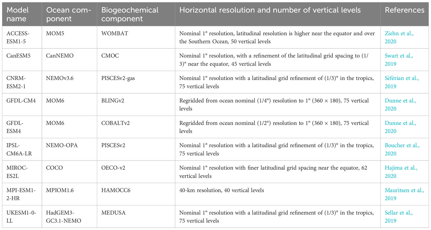
Table 1 List of CMIP6 ESMs used in the study.

2.2 Research domain

The study focuses on the coastal region of the California Current from northern Mexico to the southern tip of Vancouver Island (30°N to 48°N). We define a 2° belt along the coast as the coastal region (Figure 1). The coastal region is further divided into three subregions by Cape Mendocino and Point Conception, including the north (40.4°N to 48°N), central (34.5°N to 40.4°N), and south (30°N to 34.5°N). Averaged time series within each subregion were analyzed separately because of distinct characteristics in upwelling and biogeochemical processes from north to south (Huyer, 1983; Checkley and Barth, 2009). We might expect different trends in these subregions due to future changes in the location of the North Pacific High and its potential effect on upwelling (Rykaczewski et al., 2015). To show the coastal DO in a larger context, we also examined the spatial patterns of DO in the extended domain (28°N to 50°N, 115°W to 130°W).

FIGURE 1

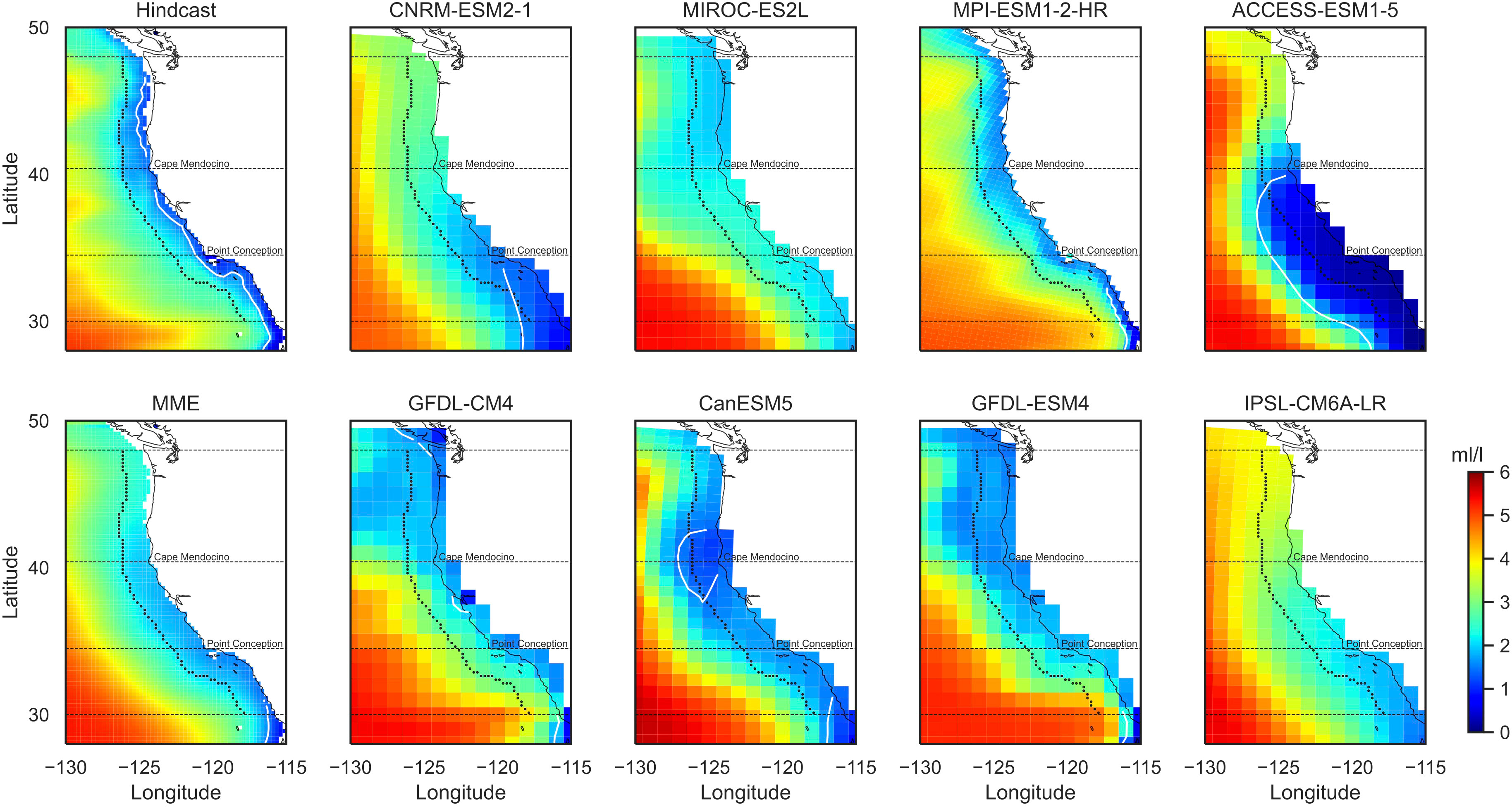
Figure 1 Summer dissolved oxygen at 200-m-depth level for 1993–2020. Shown are mean fields from hindcast, eight CMIP6 models, and the multi-model ensemble (MME). The dashed black curve/lines outline the coastal band and three subregions. The white curve is the hypoxia threshold (1.4 mL/L).

2.3 Definition of hypoxia

Hypoxia is usually defined when DO concentration is lower than the threshold of 1.4 mL/L. However, using a fixed threshold for model simulations that have biases in their representation of mean DO concentrations results in unreasonable hypoxia patterns (see Discussion). Therefore, we adjusted the hypoxic threshold on the basis of the summer climatology in the hindcast and propose a relative hypoxic threshold defined as the ratio between 1.4 mL/L and the climatological mean summer DO. For each grid point, we define.

$\begin{array}{ll}Relative thres. = 1.4/D{O}_{hindcast clim,}& \text{Eq. (1)}\end{array}$

where $D{O}_{hindcast clim.}$ is the summer climatology in the hindcast for the period of 1993 to 2020. This approach effectively tailors the threshold for hypoxia to the biases in each model climatology in comparison with the hindcast climatology. The relative thresholds (Supplementary Figure 5) are higher (more frequently reached), where the climatological DO is low. This is most evident along the coastline. However, a negative DO bias in the hindcast when compared with direct observations (e.g., at 100-m depth in the northern subregion; Supplementary Figure 3) would lead to higher thresholds and thus overestimating hypoxia frequencies.

The relative thresholds (Supplementary Figure 5) are used to identify hypoxic conditions in each model, i.e., the ratio between summer DO and model climatology is lower than the relative threshold. This approach is equivalent to bias correcting the model climatology through adjusting the threshold for each model. It yields reasonable patterns of present-day hypoxia frequency compared with the hindcast.

In addition to using the relative threshold for hypoxia, we also adjusted the variability of the CMIP6 outputs based on the summer DO variability in the hindcast. This is necessary because the variability in each model’s simulated DO is generally lower than that in the hindcast (Figure 2; Supplementary Figure 8), and this would lead to an underestimation (overestimation) of hypoxia frequency when the mean DO level is high (low). To do this, we first removed the mean summer DO ($D{O}_{cont.clim.}$) in the models for each grid point to obtain the summer DO anomalies ($D{O}_{anom.}$); then, we multiplied the summer DO anomalies with the ratio of standard deviations between the hindcast and individual models for each grid point for the period of 1993 to 2020; lastly, we added back the DO climatology to obtain the bias-adjusted summer DO concentrations ($D{O}_{adj.}$). To take into account of long-term trends in DO projections, we used the contemporaneous climatology ($D{O}_{cont.clim.}$) within a 30-year running window. The anomalies during the 15 years at each end of the time span were calculated using the 30-year window at each end, respectively.

FIGURE 2

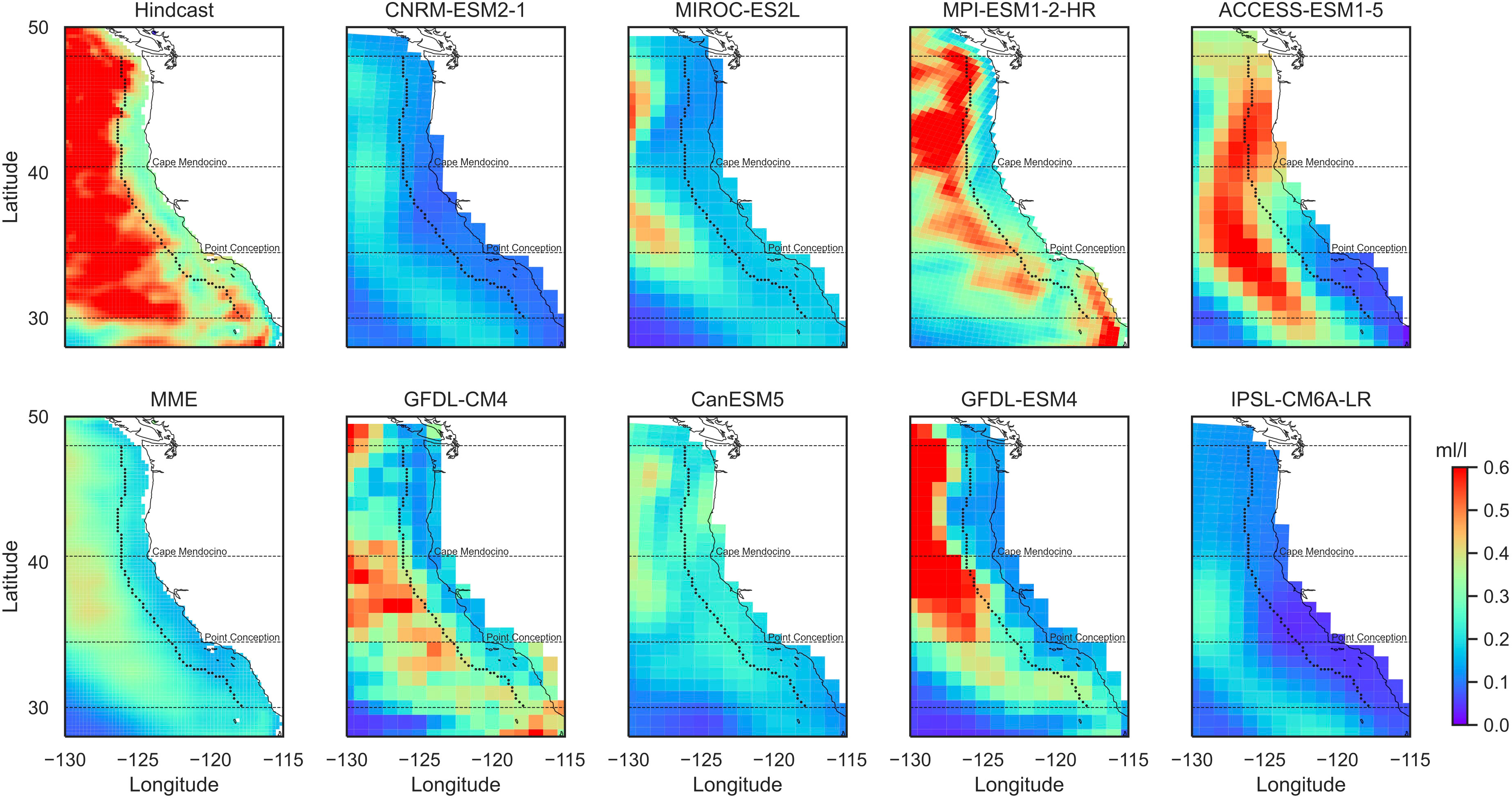
Figure 2 Variability of summer dissolved oxygen at 200-m-depth level for 1993–2020. Shown are standard deviations from hindcast, eight CMIP6 models, and the multi-model ensemble (MME). The dashed black curve/lines outline the coastal band and three subregions.

$\begin{array}{ll}D{O}_{anom.}=D{O}_{summer}-D{O}_{cont.clim.},& \text{Eq. (2)}\end{array}$

$\begin{array}{ll}D{O}_{adj.} =D{O}_{cont.clim.}+ D{O}_{anom.}*(\frac{D{O}_{hindcast stdv.}}{D{O}_{model stdv.}}),& \text{Eq. (3)}\end{array}$

These approaches provide an empirical way to correct the biases in models’ climatological means and variances, to account for the fixed threshold with model spread, and to ensure proper amplitude of internal variability of modeled DO. These adjustments linearly amplify/reduce the magnitudes of the model mean and variance by a factor of the ratio between model and hindcast climatological mean DO/internal DO variability. We are aware that these adjustments are done on the basis of the assumption that the model biases are stationary through time (Krinner and Flanner, 2018; Krinner et al., 2020). However, the window that we used as the historical period is limited by the available hindcast time span (1993–2020) and subject to decadal variability, and, thus, the benefit of the bias adjustments might be affected (see Discussion).

Hypoxia frequency is then defined as the number of summers per decade that a certain grid point is under hypoxic conditions as represented by the seasonal average.

$\begin{array}{ll}Hypoxia freq. = \frac{N_{summer}(D{O}_{adj.}/D{O}_{model clim.}<Relative thres.)}{10 years},& \text{Eq. (4)}\end{array}$

where $D{O}_{adj.}$ is the summer DO concentrations in the ESMs, $D{O}_{model clim.}$ is the model summer DO climatology for the period of 1993 to 2020, $N_{summer}$ is the number of hypoxic summers in every 10 years defined on the basis of the relative threshold. The regional hypoxia frequency is then obtained by averaging the summer hypoxic frequencies within each subdomain defined in Section 2.2.

Note that these adjustments were only made for the analysis of hypoxia frequency. The summer DO discussed in the results section are not bias-adjusted. We intend to show the relatively large spread in the direct outputs across the ESMs and to provide a way to obtain relatively consistent estimates of the hypoxia conditions with these outputs.

3 Results

3.1 Summer dissolved oxygen in the CMIP6 ESMs and hindcast

Summer DO in the subsurface waters from the hindcast shows an increasing gradient from the coast to the open ocean (Figure 1; Supplementary Figure 6). At 100-m-depth level, hypoxic conditions (DO< 1.4 mL/L) are found very close to the coast and largely in the North (Supplementary Figure 6). At 200-m-depth level, hypoxic conditions are found along the entire coast, except regions near Cape Mendocino (Figure 1). Lower DO is found in the southern subregion close to the coast (Figure 1). Simulations from the CMIP6 models all show the increasing gradients in DO from the coast to the open ocean as in the hindcast, despite the substantial differences in spatial patterns among the models (Figure 1; Supplementary Figure 6). At 100-m-depth level, the hypoxic conditions in the North are not captured by any of the CMIP6 models due to an overestimation of coastal DO in this region (Supplementary Figure 6). ACCESS-ESM1-5 reproduces the hypoxia in the central California Current, but with a much larger extent (Supplementary Figure 6). At 200-m-depth level, several models simulate hypoxic conditions in the South but in much larger areas (CNRM-ESM2-1 and ACCESS-ESM1-5; Figure 1). Models that simulate hypoxic conditions in the northern and central coast generally underestimate DO in these regions (GFDL-CM4 and CanESM5). Models that simulate lower DO in the North (MIROC-ES2L, GFDL-CM4, and GFDL-ESM4; Figure 1) tend to miss the continental shelf or have a narrower one in the North (Supplementary Figure 7). Overall, MPI-ESM1-2-HR simulates coastal patterns most similar to the hindcast (Figure 1; Supplementary Figure 6), although it still overestimates DO along the northern and central coast, as well as in the open ocean for the 200-m-depth level (Figure 1). The MME captures the general patterns of DO in the hindcast in the larger domain; but it produces weaker gradients in the coastal region (Figure 1; Supplementary Figure 6). For 200-m-depth level, the MME overestimates coastal DO especially in the North (Figure 1).

Variability of summer DO at 200-m-depth level in the hindcast shows a sharp increase from the 2° coastal band to the open ocean (Figure 2). This distinguishes significantly from the 100-m-depth level (Supplementary Figure 8), where relatively higher summer DO variability is found in the coastal zone than the open ocean, especially in the Central and South regions. Most CMIP6 models capture the change in DO variability from the coast to the open ocean (Figure 2; Supplementary Figure 8). For the 100-m depth, most models simulate strong variability in the North but tend to underestimate variability in the southern coastal zone (Supplementary Figure 8). At 200-m depth, almost all models underestimate the variability within the 2° coast band (Figure 2). The MMEs underestimate the summer DO variability compared with the hindcast, but they were able to capture the general patterns of the DO variability for both depth levels (Figure 2; Supplementary Figure 8).

At 100-m depth, the regional averaged DO in the hindcast is higher in the South than in the North and Central (Figure 3). Compared with the hindcast, the MME slightly overestimates the DO but the hindcast is within the model spread (one standard deviation). For the 200-m depth, the regional averaged DO in the hindcast is close to the hypoxic level for all three subregions (Figure 3). The MME agrees well with the hindcast, especially for the Central and the South. In the North, MME overestimates the DO but the hindcast is still within the model spread.

FIGURE 3

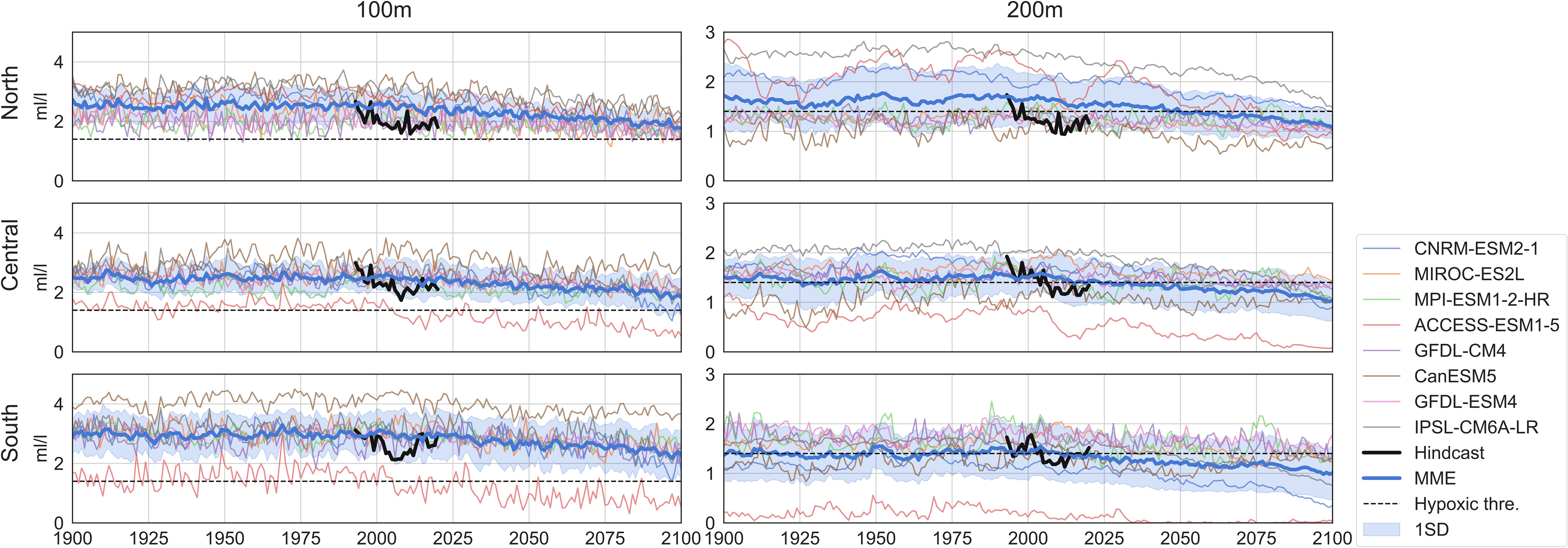
Figure 3 Averaged summer dissolved oxygen in coastal California Current (2° band). The time series are from hindcast (black), eight CMIP6 models (multiple colors), and the multi-model ensemble (MME, blue). The blue shading is the one standard deviation across ensemble members. The dashed line is the hypoxia threshold (1.4 mL/L). Three subregions shown are the North (top), Central (middle) and South (bottom), and two depth levels are the 100 m (left panel) and 200 m (right panel).

3.2 Summer hypoxia in the CMIP6 ESMs and hindcast

Climatological summer hypoxia frequencies (Figure 4) are generated with bias adjusted DO [Equation (4)] to obtain comparable patterns across the models. Summer hypoxia in the hindcast mainly occurs along the coastal regions at the 200-m-depth level, and higher frequencies are found in the South (Figure 4). Most of the CMIP6 models were able to simulate the coastal hypoxia occurrence with relatively higher frequencies in the South. Within the coastal band, the MME captures the spatial distribution of hypoxia frequencies well compared with the hindcast, although it overestimates the frequencies in the north on the continental shelf. At the 100-m-depth level, summer hypoxia was only found very close to the coast in the hindcast in the North and Central subregions and just south of Point Conception (Supplementary Figure 9). All CMIP6 models were able to simulate these regions of hypoxia occurrences. The spatial pattern in the MME also largely resembles that of the hindcast.

FIGURE 4

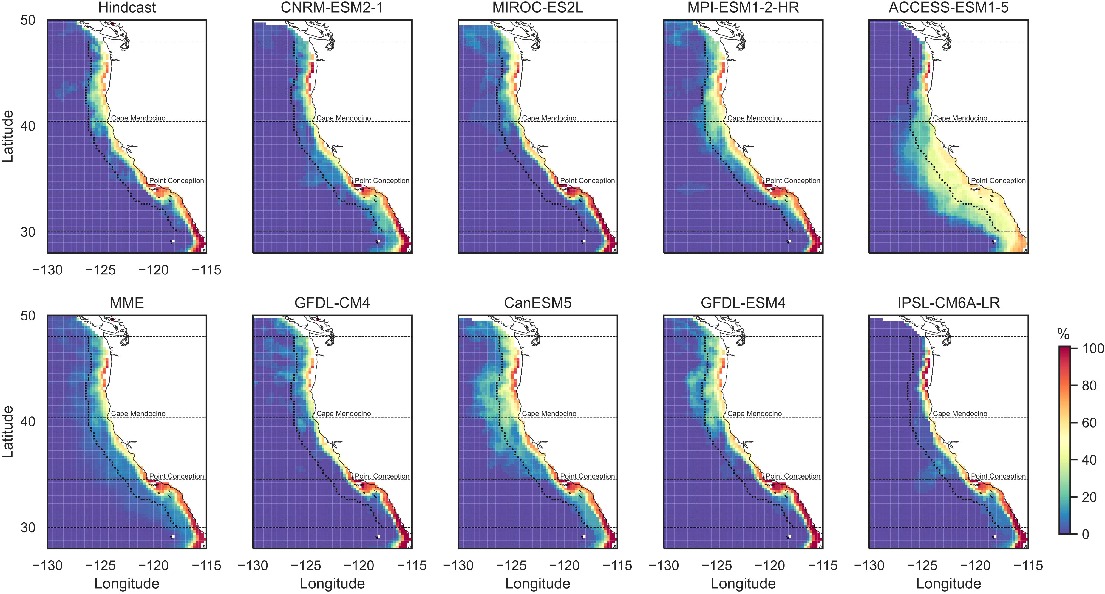
Figure 4 Summer hypoxia frequencies (%) for the 200-m depth during 1993–2020. Shown are results from hindcast, eight CMIP6 models, and the multi-model ensemble (MME). The dashed black curve/lines outline the coastal band and three subregions. Frequency is defined as the number of summers per decade that are under hypoxic condition and is represented in percentage.

Averaged summer hypoxia frequencies for the recent decades (1993–2020) in MME agree quite well with those in the hindcast for all three coastal subregions (Figure 5). Slightly larger differences are found in the North and South subregions for the 200-m-depth level, but the averaged hypoxia frequencies in the hindcast are generally within the model spread for most subregions.

FIGURE 5

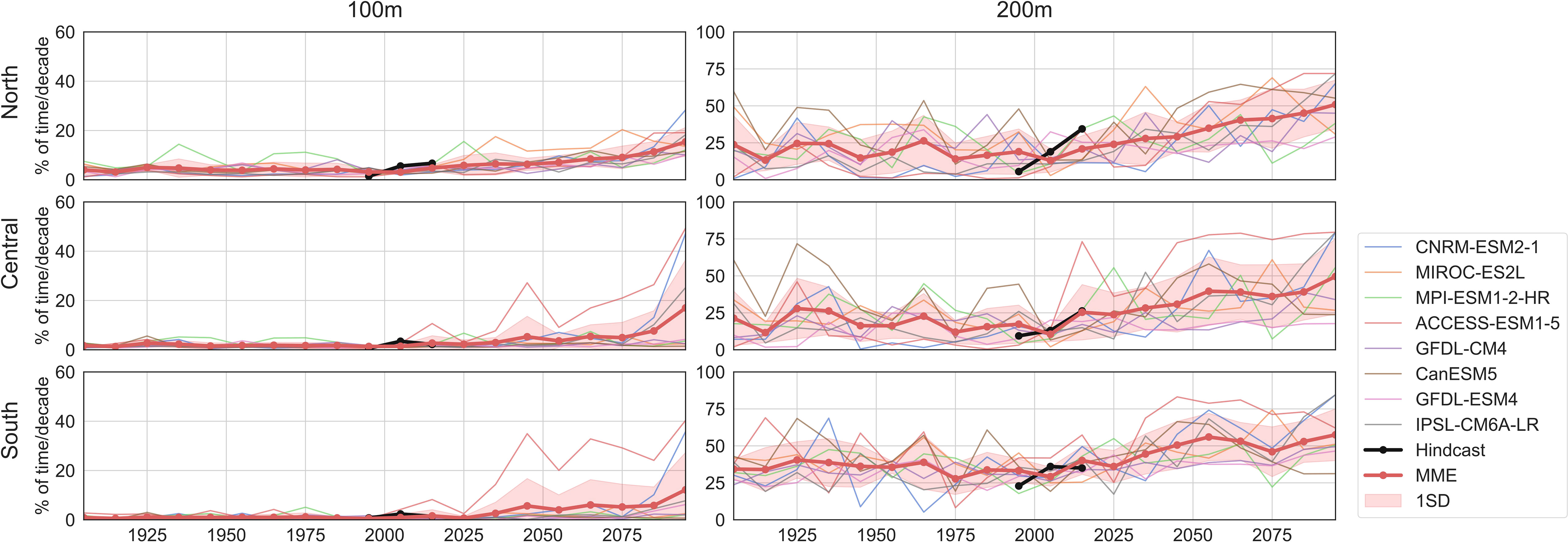
Figure 5 Averaged summer hypoxia frequencies in coastal California Current (2° band). The time series are from hindcast (black), eight CMIP6 models (multiple colors), and the multi-model ensemble (MME, red). The red shading is the one standard deviation across ensemble members. Three subregions shown are the North (top), Central (middle), and South (bottom), and two depth levels are the 100 m (left panel) and 200 m (right panel).

3.3 Future change in summer hypoxia

Future summer hypoxia frequencies (Figure 5) are calculated after applying bias adjustments [Equation (4)] to the projected DO. Summer hypoxia is projected to be more frequent in the coastal California Current for both depth levels in response to warming (Figure 5). This is consistent with the significant decreasing trends in summer DO across the 21st century (Figure 3; Supplementary Tables 2, 3). By the end of the 21st century, the MME shows that about 10%–15% of summers will be under hypoxic conditions at 100 m for the coastal regions. At 200 m, the summer hypoxia frequency is projected to reach about 50% for the North and Central and about 65% for the South, compared with the present frequencies of about 15% in North and Central and about 30% in the South. For the 100-m depth, ACCESS-ESM1-5 tends to project high hypoxia frequencies especially in the South, likely due to its strong decreasing trend in the summer DO in this subregion (Supplementary Table 2). CNRM-ESM2-1 projects high hypoxia frequencies after around 2075, and this might be related to a nonlinear decrease in the DO around that time period (Figure 3). For the 200-m depth, CanESM5 tends to simulate high hypoxia frequencies, and this could be related to the large decadal variability in the simulated summer DO (Figure 3). Similarly, MIROC-ES2L with larger decadal DO variability (Figure 3) also projects high hypoxia frequencies in the North. ACCESS-ESM1-5, which simulates large regions with relatively high (40%–60%) historical hypoxia frequencies in the Central and South (Figure 4), projects high frequencies in these regions for the future decades. For both depth levels, MPI-ESM-1-2-HR seems to simulate high variability and smaller increasing trends, projecting lower frequencies at the 200-m depth after around 2060 (Figure 5).

Spatially, summer hypoxia is projected to occur more frequently across the coastal band and extending to the open ocean at 200 m by the end of the 21st century (Figure 6). This is consistent with the projected decreases in DO in the California Current (Supplementary Figure 10). At the 100-m-depth level, increased hypoxia frequencies are found mostly within the coastal band. Strongest increases up to about 60% are found in the North in regions immediately off the continental shelf. By the end of the 21st century, up to 100% summer hypoxia occurrence along the coast and about 10%–15% across the coastal band are projected. At the 200-m-depth level, up to 60% increases in hypoxia frequencies are found over the coastal California Current, from immediately off the continental shelf to the open ocean. By the end of the 21st century, hypoxia frequencies are projected to reach 100% along the coast across the entire domain. Outside the coastal band where there is no hypoxia stimulated during the historical period, hypoxia frequencies are projected to be about 15%–20%.

FIGURE 6

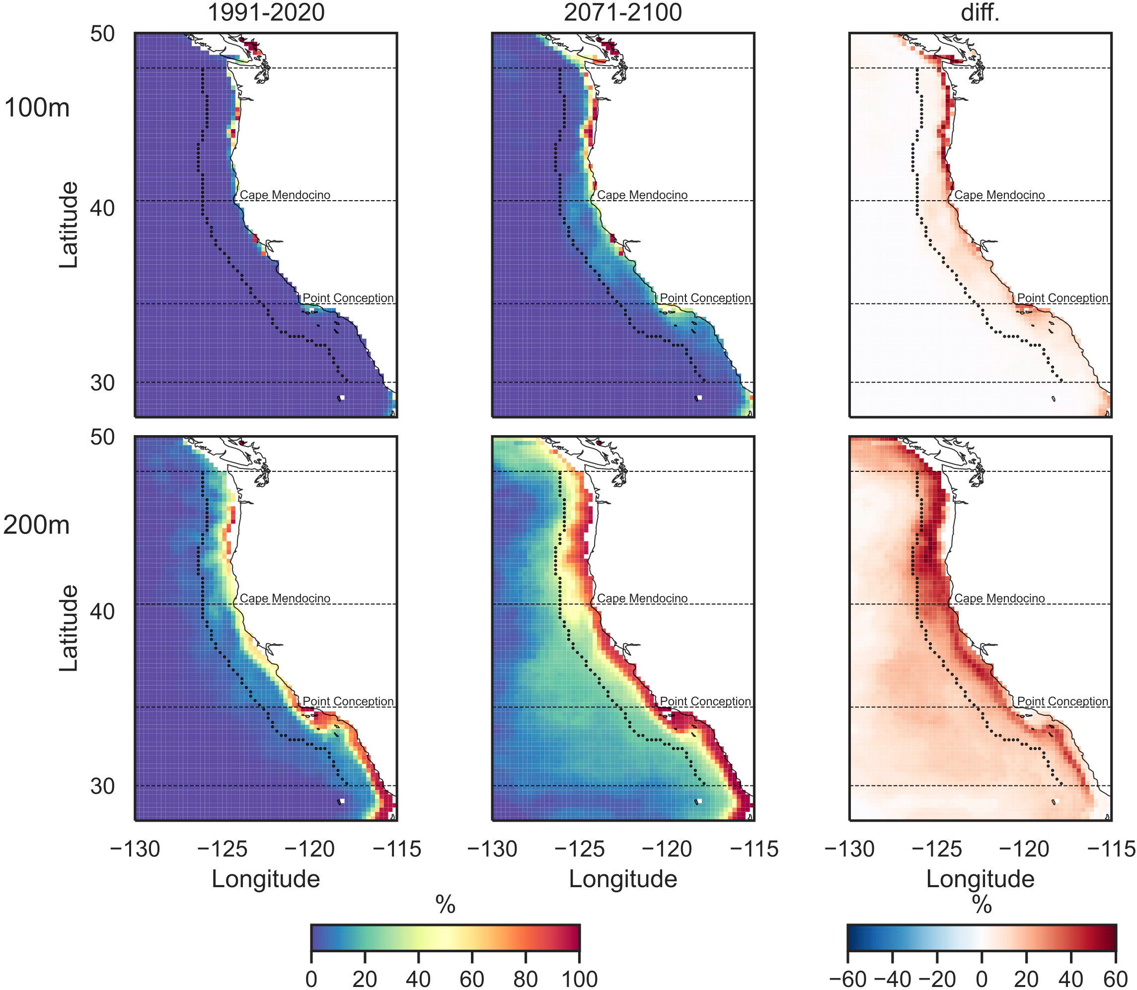
Figure 6 Historical (1993–2020, left) and future (2073–2100, middle) summer hypoxia frequencies and their changes (right). Shown is the multi-model ensemble from eight CMIP6 models. Two depth levels are the 100 m (top panel) and 200 m (bottom panel). The dashed black curve/lines outline the coastal band and three subregions.

4 Summary and discussion

In this study, we examined the summer DO and hypoxia frequency in the California Current and its coastal domain with an ensemble of the new generation ESMs. We found that the ESMs show various degrees of agreement with the hindcast in simulated summer DO climatology (Figure 1). The ESMs underestimate summer-to-summer variance of the DO in comparison to the hindcast (Figure 2). For the summer DO in the coastal region, the MME generally agrees with the hindcast, but the model spread is large (Figure 3). ESM simulations of oxygen concentrations under present-day conditions and into the future are quite variable. However, after necessary bias adjustments, uncertainties related to different model native grids, interpolation, and bathymetry can be effectively mitigated to generate relatively consistent hypoxia frequency and patterns for the coastal California Current (Figures 4–6).

Toward the end of the 21st century, models project consistent increase in the summer hypoxia frequencies in the coastal region of California Current (Figure 5). Increases in hypoxia frequency are projected to be off the continental shelf (Figure 6). This is because over the continental shelf, hypoxia frequency in some regions already reaches 100% under present-day conditions as simulated by the hindcast, e.g., in the southern coastal California Current (Figure 4). Therefore, the future projections show a band of near zero change in hypoxia frequency along the coast with climate change, as the frequency of hypoxia is already high. However, these results should be interpreted taking into consideration the accuracy of the hindcast. The coastal DO biases in the hindcast for the northern subregion (Supplementary Figures 1–3) would potentially lead to an overestimation of hypoxia frequency in the present day and, thus, an underestimate of the magnitude of increases along the northern coastal band into the future.

Hypoxia by definition has an absolute threshold; thus, the long-term decline in DO will lead to increase in hypoxia frequency. While an ensemble analysis of the DO is reasonable, analyzing the hypoxia frequencies with the ensemble approach is not directly feasible because the absolute hypoxic threshold would lead to obvious error due to the large spread across the ESMs. The bias correction proposed in the study provides an empirical way to address this issue, facilitating an ensemble analysis of the hypoxia frequencies and their future changes. Without the application of the relative threshold, unrealistic patterns of hypoxia would be generated compared with the hindcast (Supplementary Figures 11, 12). In most models, the DO is systematically high along the coast (Figure 1; Supplementary Figure 6), leading to no coastal hypoxia detected with the absolute threshold of 1.4 mL/L (Supplementary Figures 11, 12). In models with low DO climatology, e.g., ACCESS-ESM1-5, an extended area of high hypoxia frequency is simulated in southern and central California Current (Supplementary Figures 11, 12). The application of relative threshold does lead to significant changes in the hypoxia patterns compared to those identified with the absolute threshold of 1.4 mL/L even for the same model. However, we point out that these changes are reasonable and lead to better resemblance of the reference hypoxia patterns in the hindcast. On top of the long-term trend, the variability of the DO also modifies the hypoxia frequency, and it needs to be properly adjusted for each individual model before the ensemble. Without correction for the variance, most models underestimate the coastal hypoxia frequency (Supplementary Figure 13) due to the overall underestimation of the DO variance in comparison to the hindcast (Figure 2; Supplementary Figures 8, 14). Spatially, the models simulate very high hypoxia frequencies (100%) largely confined to the narrow zone immediately off the coast due to very low DO variability in these areas (Supplementary Figures 15, 16). Majority of the models underestimates the hypoxia frequency away from the coastline within the 2° coastal band (Supplementary Figure 15). One caveat is that the bias adjustment approach is sensitive to decadal variability of each model. If the baseline period in the model exhibits anomalously high (low) DO concentrations due to decadal variability, then the bias adjustment approach would lead to a high (low) bias in hypoxia frequency. This issue could be addressed through analysis of a single-model large ensemble in which the influence of decadal variability can be removed. Other techniques, e.g., to filter low frequency variability before bias adjustment, can also be applied to further explore the role of decadal variability. Lastly, the bias adjustment method used here is an empirical approach that was tailored for the specific question of changes in the frequency of low-oxygen events during the summer time. Whether such an approach could be applied to other types of extreme events requires further consideration. Projecting changes in the frequency of hypoxia using output from these earth-system models is a rather specific challenge. Using a fixed threshold for hypoxia is not possible because of model biases to the mean state. Simply adjusting the model output to remove the mean bias is not sufficient to properly identify extremes. The method applied (i.e., using a model-specific threshold while scaling oxygen variance using best estimates of internal variance) was meant to be a pragmatic approach to addressing these issues. Future application of this approach requires judgment for suitability.

One limitation of the study is that the accuracy of the results depends on the quality of baseline climatology selected. The choice of the hindcast data as the baseline for the study is not ideal, as biases exist between the hindcast and observations, especially along the coast (Supplementary Figures 1–3). However, a portion of these biases is related to the low spatial resolution in the existing observationally based climatologies. There are also uncertainties among observationally based datasets (Supplementary Figures 1–3, Supplementary Table 1). In the southern subregion, a very good agreement between the hindcast and observations from the CalCOFI survey is found for both the mean DO and its variability (Supplementary Figure 3). In addition, identifying hypoxia frequencies requires not only the climatology but also the variability of the DO. The existing observationally based datasets usually lack information on DO variances for the targeted season. Sources that provide DO variability, e.g., observations from the CalCOFI survey and the Newport Hydrographic Line, are extremely valuable but cover very limited areas of the California Current. This also highlights the need for more spatially comprehensive observational data, and high-quality time series of DO for the coastal regions. In addition, the spatial extent of hypoxia frequency still shows considerable differences across the models. In addition to differences in model biogeochemical components and parameterizations, this is likely related to the model resolutions. Given the dependence of oxygen on production and on respiration of organic matter that can be confined to the continental shelf and vary sharply with depth, bathymetry, and sub-mesoscale circulation, there is a need for high-resolution models that can more satisfactorily simulate the observed dynamics and hence project future changes.

These findings suggest that it is possible to use the CMIP6 MME to project regional biogeochemical change, as the individual models provide a consistent story of deoxygenation trends, in this case of California Current. With proper adjustment of individual model variability, the MME provides relatively consistent estimates of hypoxia frequencies, in terms of their spatial patterns and trends in the coastal region. These results are broadly similar to those found in dynamically downscaled regional models (Pozo Buil et al., 2021), where shoaled hypoxic boundaries are projected in the California Current, especially along the coastline with extended areas in the northern and central subregions, as well as the weak change in hypoxic boundaries over the continental shelf. Results from the downscaled Hadley Center HadGEM2-ES (from the CMIP5 archive) show increased DO along the coastal California Current, which is the opposite from our analysis. However, the model from Hadley Center (UKESM1-0-LL, from the CMIP6 archive) is excluded as an outlier from our analysis (see Materials and methods). The near 100% summer hypoxia in some regions under present-day conditions and in the future will mean that pelagic and benthic habitat along the US West Coast will be greatly affected, resulting potentially in local extinctions of some species, shifting species distributions (deeper or offshore), and large changes in community structure in the California Current.

Data availability statement

The original contributions presented in the study are included in the article/Supplementary Material. Further inquiries can be directed to the corresponding author.

Author contributions

HS, SB, MG-R, MJ, BB, WS, and RR discussed and designed the research. HS obtained the data and conducted the analysis. HS, RR, MP, and SB wrote the initial draft of the manuscript and all authors participated in editing the manuscript for clarity and brevity. All authors contributed to the article and approved the submitted version.

Funding

This study was supported by NOAA’s Climate Program Office’s Modeling, Analysis, Predictions, and Projections Program, Grant # NA19OAR4310290 and Grant # NA20OAR4310447.

Acknowledgments

We thank Copernicus Marine Service and Mercator Ocean for making the Global Ocean Biogeochemistry Hindcast available (https://doi.org/10.48670/moi-00019). We thank NOAA National Centers for Environmental Information for making the World Ocean Atlas 2018 data available. We thank CSIRO Oceans & Atmosphere – Hobart for making the CSIRO Atlas of Regional Seas 2009 available. We thank the CERN, the OpenAIRE project, and Zenodo for providing open access to the Newport Hydrographic Line observations. We thank the California Cooperative Oceanic Fisheries Investigations for making the CalCOFI data available and thank I. Schroeder for preparing and preprocessing the data. We acknowledge the World Climate Research Program’s Working Group on Coupled Modeling for providing the CMIP6 model outputs.

Conflict of interest

The authors declare that the research was conducted in the absence of any commercial or financial relationships that could be construed as a potential conflict of interest.

Publisher’s note

All claims expressed in this article are solely those of the authors and do not necessarily represent those of their affiliated organizations, or those of the publisher, the editors and the reviewers. Any product that may be evaluated in this article, or claim that may be made by its manufacturer, is not guaranteed or endorsed by the publisher.

Supplementary material

The Supplementary Material for this article can be found online at: https://www.frontiersin.org/articles/10.3389/fmars.2023.1205536/full#supplementary-material

References

Atkins J., Andrews O., Frenger I. (2022). Quantifying the contribution of ocean mesoscale eddies to low oxygen extreme events. Geophysical Res. Lett. 49 (15), e2022GL098672. doi: 10.1029/2022GL098672

CrossRef Full Text | Google Scholar

Bograd S. J., Castro C. G., Lorenzo E. D., Palacios D. M., Bailey H., Gilly W., et al. (2008). Oxygen declines and the shoaling of the hypoxic boundary in the California current. Geophysical Res. Lett. 35 (12), L12607. doi: 10.1029/2008GL034185

CrossRef Full Text | Google Scholar

Bograd S. J., Checkley D. A., Wooster W. S. (2003). CalCOFI: A half century of physical, chemical, and biological research in the California current system. Deep Sea Res. Part II: Topical Stud. Oceanography 50 (14–16), 2349–2353. doi: 10.1016/S0967-0645(03)00122-X

CrossRef Full Text | Google Scholar

Bograd S. J., Jacox M. G., Hazen E. L., Lovecchio E., Montes I., Pozo Buil M., et al. (2023). Climate change impacts on eastern boundary upwelling systems. Annu. Rev. Mar. Sci. 15 (1), 303–285. doi: 10.1146/annurev-marine-032122-021945

CrossRef Full Text | Google Scholar

Bograd S. J., Pozo Buil M., Di Lorenzo E., Castro C. G., Schroeder I. D., Goericke R., et al. (2015). Changes in source waters to the Southern California bight. Deep Sea Res. Part II: Topical Stud. Oceanography 112 (February), 42–52. doi: 10.1016/j.dsr2.2014.04.009

CrossRef Full Text | Google Scholar

Bograd S. J., Schroeder I. D., Michael G. J. (2019). A water mass history of the Southern California current system. Geophysical Res. Lett. 46 (12), 6690–6985. doi: 10.1029/2019GL082685

CrossRef Full Text | Google Scholar

Boucher O., Servonnat J., Albright A. L., Aumont O., Balkanski Y., Bastrikov V. (2020). Presentation and evaluation of the IPSL-CM6A-LR climate model. J. Adv. Modeling Earth Syst. 12, e2019MS00201. doi: 10.1029/2019MS002010

CrossRef Full Text | Google Scholar

Breitburg D., Levin L. A., Oschlies A., Grégoire M., Chavez F. P., Conley D. J., et al. (2018). Declining oxygen in the global ocean and coastal waters. Science 359 (6371), eaam7240. doi: 10.1126/science.aam7240

PubMed Abstract | CrossRef Full Text | Google Scholar

Chan F., Barth J. A., Kroeker K. J., Lubchenco J., Menge. B. A. (2019). THE DYNAMICS AND IMPACT OF OCEAN ACIDIFICATION AND HYPOXIA: insights from sustained investigations in the Northern California current large marine ecosystem. Oceanography 3, 62–71. doi: 10.5670/oceanog.2019.312

CrossRef Full Text | Google Scholar

Chan F., Barth J. A., Lubchenco J., Kirincich A., Weeks H., Peterson W. T., et al. (2008). Emergence of anoxia in the California current large marine ecosystem. Science 319 (5865), 920–920. doi: 10.1126/science.1149016

PubMed Abstract | CrossRef Full Text | Google Scholar

Checkley D. M., Barth J. A. (2009). Patterns and processes in the California current system. Prog. Oceanography 83 (1–4), 49–64. doi: 10.1016/j.pocean.2009.07.028

CrossRef Full Text | Google Scholar

Cheresh J., Fiechter J. (2020). Physical and biogeochemical drivers of alongshore PH and oxygen variability in the California current system. Geophysical Res. Lett. 47 (19), e2020GL08955. doi: 10.1029/2020GL089553

CrossRef Full Text | Google Scholar

Dunne J. P., Horowitz L. W., Adcroft A. J., Ginoux P., Held I. M., John J. G., et al. (2020). The GFDL earth system model version 4.1 (GFDL-ESM 4.1): overall coupled model description and simulation characteristics. J. Adv. Modeling Earth Syst. 12 (11), e2019MS00201. doi: 10.1029/2019MS002015

CrossRef Full Text | Google Scholar

Dussin R., Curchitser E. N., Stock C. A., Van Oostende N. (2019). Biogeochemical drivers of changing hypoxia in the California current ecosystem. Deep Sea Res. Part II: Topical Stud. Oceanography 169–170, 104590. doi: 10.1016/j.dsr2.2019.05.013

CrossRef Full Text | Google Scholar

Echevin V., Gévaudan M., Espinoza-Morriberón D., Tam J., Aumont O., Gutierrez D., et al. (2020). Physical and biogeochemical impacts of RCP8.5 scenario in the Peru upwelling system. Biogeosciences 17 (12), 3317–3415. doi: 10.5194/bg-17-3317-2020

CrossRef Full Text | Google Scholar

Evans N., Schroeder I. D., Pozo Buil M., Jacox M. G., Bograd S. J. (2020). Drivers of subsurface deoxygenation in the Southern California current system. Geophysical Res. Lett. 46, 2020GL08927. doi: 10.1029/2020GL089274

CrossRef Full Text | Google Scholar

Eyring V., Bony S., Meehl G. A., Senior C. A., Stevens B., Stouffer R. J., et al. (2016). Overview of the coupled model intercomparison project phase 6 (CMIP6) experimental design and organization. Geoscientific Model. Dev. 9, 1937–1958 doi: 10.5194/gmd-9-1937-2016

CrossRef Full Text | Google Scholar

Fennel K., Testa J. M. (2019). Biogeochemical controls on coastal hypoxia. Annu. Rev. Mar. Sci. 11 (1), 105–305. doi: 10.1146/annurev-marine-010318-095138

CrossRef Full Text | Google Scholar

Frölicher T. L., Rodgers K. B., Stock C. A., Cheung W. W.L. (2016). Sources of uncertainties in 21st century projections of potential ocean ecosystem stressors. Global Biogeochemical Cycles 30 (8), 1224–1435. doi: 10.1002/2015GB005338

CrossRef Full Text | Google Scholar

García H. E., Locarnini R. A., Boyer T. P., Antonov J. I., Mishonov A. V., Baranova O. K., et al. (2013). “World ocean atlas 2013 volume 3: dissolved oxygen, apparent oxygen utilization, and oxygen saturation,” in NOAA Atlas NESDIS 75, vol. 27. Eds. Levitus S., Mishonov A.. Available at: http://www.nodc.noaa.gov/OC5/indprod.html.

Google Scholar

García H. E., Weathers K., Paver C. R., Smolyar I., Boyer T. P., Locarnini R. A., et al. (2019). “World ocean Atlas 2018, volume 3: dissolved oxygen, apparent oxygen utilization, and oxygen saturation,” in NOAA atlas NESDIS 83, vol. 38 pp. Ed. Mishonov A.. Available at: https://www.nodc.noaa.gov/OC5/woa18/pubwoa18.html.

Google Scholar

García-Reyes M., Sydeman W. J., Schoeman D. S., Rykaczewski R. R., Black B. A., Smit A. J., et al. (2015). Under pressure: climate change, upwelling, and eastern boundary upwelling ecosystems. Front. Mar. Sci. 2 (December). doi: 10.3389/fmars.2015.00109

CrossRef Full Text | Google Scholar

Grantham B. A., Chan F., Nielsen K. J., Fox D. S., Barth J. A., Huyer A., et al. (2004). Upwelling-driven nearshore hypoxia signals ecosystem and oceanographic changes in the Northeast Pacific. Nature 429 (6993), 749–754. doi: 10.1038/nature02605

PubMed Abstract | CrossRef Full Text | Google Scholar

Hajima T., Watanabe M., Yamamoto A., Tatebe H., Noguchi M. A., Abe M., et al. (2020). Development of the MIROC-ES2L Earth system model and the evaluation of biogeochemical processes and feedbacks. Geoscientific Model. Dev. 13 (5), 2197–2244. doi: 10.5194/gmd-13-2197-2020

CrossRef Full Text | Google Scholar

Huyer A. (1983). Coastal upwelling in the California current system. Prog. Oceanography. 12 (3), 259–284. doi: 10.1016/0079-6611(83)90010-1

CrossRef Full Text | Google Scholar

Krinner G., Flanner M. G. (2018). Striking stationarity of large-scale climate model bias patterns under strong climate change. Proc. Natl. Acad. Sci. 115 (38), 9462–9665. doi: 10.1073/pnas.1807912115

CrossRef Full Text | Google Scholar

Krinner G., Kharin V., Roehrig R., Scinocca J., Codron F. (2020). Historically-based run-time bias corrections substantially improve model projections of 100 years of future climate change. Commun. Earth Environ. 1, 29. doi: 10.1038/s43247-020-00035-0

CrossRef Full Text | Google Scholar

Kwiatkowski L., Torres O., Bopp L., Aumont O., Chamberlain M., Christian J. R., et al. (2020). Twenty-first century ocean warming, acidification, deoxygenation, and upper-ocean nutrient and primary production decline from CMIP6 model projections. Biogeosciences 17 (13), 3439–3470. doi: 10.5194/bg-17-3439-2020

CrossRef Full Text | Google Scholar

Mauritsen T., Bader J., Becker T., Behrens J., Bittner M., Brokopf R. (2019). Developments in the MPI-M Earth system model version 1.2 (MPI-ESM1.2) and its response to increasing CO 2 developments in the MPI-M Earth system model version 1.2 (MPI-ESM1.2) and its response to increasing CO. J. Adv. Modeling Earth Syst. 2, 11. doi: 10.1029/2018MS001400

CrossRef Full Text | Google Scholar

Meinshausen M., Nicholls Z. R.J., Lewis J., Gidden M. J., Vogel E., Freund M., et al. (2020). The shared socio-economic pathway (SSP) greenhouse gas concentrations and their extensions to 2500. Geoscientific Model. Dev. 13 (8), 3571–3605. doi: 10.5194/gmd-13-3571-2020

CrossRef Full Text | Google Scholar

O’Neill B. C., Tebaldi C., Van Vuuren D. P., Eyring V., Friedlingstein P., Hurtt G., et al. (2016). The scenario model intercomparison project (ScenarioMIP) for CMIP6. Geoscientific Model. Dev. 9 (9), 3461–3482. doi: 10.5194/gmd-9-3461-2016

CrossRef Full Text | Google Scholar

Perruche C., Szczypta C., Paul J., Drévillon M. (2019) Quality information document (QuID) - global production centre GLOBAL_REANALYSIS_BIO_001_029 copernicus marine environment monitoring service. Available at: http://catalogue.marine.copernicus.eu/documents/QUID/CMEMS-GLO-QUID-001-029.pdf.

Google Scholar

Pozo Buil M., Jacox M. G., Fiechter J., Alexander M. A., Bograd S. J., Curchitser E. N., et al. (2021). A dynamically downscaled ensemble of future projections for the California current system. Front. Mar. Sci. 8 (April). doi: 10.3389/fmars.2021.612874

CrossRef Full Text | Google Scholar

Ridgway K. R., Dunn J. R., Wilkin J. L. (2002). Ocean interpolation by four-dimensional weighted least squares—Application to the waters around Australasia. J. Atmospheric Oceanic Technol. 19 (9), 1357–1375. doi: 10.1175/1520-0426(2002)019<1357:OIBFDW>2.0.CO;2

CrossRef Full Text | Google Scholar

Risien C. M., Fewings M. R., Fisher J. L., Peterson J. O., Morgan C. A. (2022). Spatially gridded cross-shelf hydrographic sections and monthly climatologies from shipboard survey data collected along the newport hydrographic line 1997–2021. Data Brief 41 (April), 107922. doi: 10.1016/j.dib.2022.107922

PubMed Abstract | CrossRef Full Text | Google Scholar

Rykaczewski R. R., Dunne J. P., Sydeman W. J., García-Reyes M., Black B. A., Bograd S. J. (2015). Poleward displacement of coastal upwelling-favorable winds in the ocean’s eastern boundary currents through the 21st century. Geophysical Res. Lett. 42 (15), 6424–6315. doi: 10.1002/2015GL064694

CrossRef Full Text | Google Scholar

Séférian R., Berthet S., Yool A., Palmiéri J., Bopp L., Tagliabue A., et al. (2020). Tracking improvement in simulated marine biogeochemistry between CMIP5 and CMIP6. Current Climate Change Reports 6 (3), 95–119. doi: 10.1007/s40641-020-00160-0

PubMed Abstract | CrossRef Full Text | Google Scholar

Séférian R., Nabat P., Michou M., Saint-Martin D., Voldoire A., Colin J., et al. (2019). Evaluation of CNRM earth system model, CNRM-ESM2-1: role of Earth system processes in present-day and future climate. J. Adv. Modeling Earth Syst. 11 (12), 4182–4227. doi: 10.1029/2019MS001791

CrossRef Full Text | Google Scholar

Sellar A. A., Jones C. G., Mulcahy J. P., Tang Y., Yool A., Wiltshire A., et al. (2019). UKESM1: description and evaluation of the U.K. Earth system model. J. Adv. Modeling Earth Syst. 11 (12), 4513–4558. doi: 10.1029/2019MS001739

CrossRef Full Text | Google Scholar

Siedlecki S. A., Banas N. S., Davis K. A., Giddings S., Hickey B. M., MacCready P., et al. (2015). Seasonal and interannual oxygen variability on the Washington and Oregon continental shelves. J. Geophysical Research: Oceans 120 (2), 608–633. doi: 10.1002/2014JC010254

CrossRef Full Text | Google Scholar

Steinberg D. K., Carlson C. A., Bates N. R., Johnson R. J., Michaels A. F., Knap A. H. (2001). Overview of the US JGOFS Bermuda atlantic time-series study (BATS): A decade-scale look at ocean biology and biogeochemistry. Deep Sea Res. Part II: Topical Stud. Oceanography 48 (8–9), 1405–1447. doi: 10.1016/S0967-0645(00)00148-X

CrossRef Full Text | Google Scholar

Stramma L., Johnson G. C., Sprintall J., Mohrholz V. (2008). Expanding oxygen-minimum zones in the tropical oceans. Science 320 (5876), 655–658. doi: 10.1126/science.1153847

PubMed Abstract | CrossRef Full Text | Google Scholar

Swart N. C., Cole J. N.S., Kharin V. V., Lazare M., Scinocca J. F., Gillett N. P., et al. (2019). The Canadian Earth system model version 5 (CanESM5.0.3). Geoscientific Model. Dev. 12 (11), 4823–4873. doi: 10.5194/gmd-12-4823-2019

CrossRef Full Text | Google Scholar

Wahyudi A. J., Triana K., Masumoto Y., Rachman A., Firdaus M. R., Iskandar I., et al. (2023). Carbon and nutrient enrichment potential of south java upwelling area as detected using hindcast biogeochemistry variables. Regional Stud. Mar. Sci. 59 (April), 102802. doi: 10.1016/j.rsma.2022.102802

CrossRef Full Text | Google Scholar

Whitney F. A., Freeland H. J., Robert M. (2007). Persistently declining oxygen levels in the interior waters of the eastern subarctic pacific. Prog. Oceanography 75 (2), 179–995. doi: 10.1016/j.pocean.2007.08.007

CrossRef Full Text | Google Scholar

Ziehn T., Chamberlain M. A., Law R. M., Lenton A., Bodman R. W., Dix M., et al. (2020). The Australian earth system model: ACCESS-ESM1.5. J. South. Hemisphere Earth Syst. Sci. 70 (1), 1935. doi: 10.1071/ES19035

CrossRef Full Text | Google Scholar