Optimization of the k-nearest-neighbors model for summer Arctic Sea ice prediction

1 Introduction

Sea ice is important for climate processes such as heat, momentum, and material exchange between the ocean and the atmosphere (Lindsay et al., 2008; Steele et al., 2008). It also has a variety of ecological and social impacts, for example, the melting of sea ice affects species interaction, population mixing, productivity, and disease transmission (Post et al., 2013).

In recent years, the marked decline in Arctic sea ice extent (SIE; defined as the area of the ocean where the sea ice concentration is more than 15%) has caused widespread international concern (Stroeve et al., 2012; Kwok, 2018; Stroeve & Notz, 2018). The smallest decline occurred in winter, while the largest occurred in September. The trend for September over the period 1979-2017 was -83,000 km²/year, or -13.0% per decade when compared to the average extent for 1981-2010 (Serreze & Meier, 2019). The loss of sea ice has transformed the once unnavigable Arctic region into a seasonally navigable region (Melia et al., 2016). Affected by sea ice seasonal fluctuations, forecasting of sea ice in summer is vital to the safety and efficiency of navigation in the Arctic (Vihma, 2014; Wang et al., 2019; Chen et al., 2020; Min et al., 2022). Accurate sea ice forecasts in the summer months can also aid in mitigating potential hazards posed to navigation, such as navigation delays, collisions, and navigation errors. Furthermore, reliable predictions of SIE enable better planning and resource allocation for Arctic shipping endeavors, helping to ensure that the safest and most economical routes are used.

Since 2008, the Sea Ice Prediction Network (SIPN) has been collecting predictions of Arctic September SIE from contributors around the world (Bhatt et al., 2022a). SIPN has requested participants to submit their predicted September Arctic SIE during early June, July, August, and September. Through these submissions, SIPN provides an indication of the current prediction status of summer Arctic sea ice on the sub-seasonal-to-seasonal (S2S) timescale. Most contributors utilize dynamic models and statistical models. However, according to the predictive September SIEs submitted to SIPN, accurately predicting the Arctic SIE and spatial distribution of Arctic sea ice concentration (SIC) on the S2S timescale is still challenging, especially in September when SIE is at its minimum for the year (Wei et al., 2021).

With the recent advances in machine learning techniques, machine learning has been widely applied to Earth system analyses in recent years (Reichstein et al., 2019), which has resulted in substantial progress in the forecasting of Arctic sea ice. Chi and Kim (2017) used a fully data-driven deep learning long short-term memory (LSTM) model to predict the monthly Arctic sea ice in 2015. Jun Kim et al. (2020) used a convolutional neural network (CNN), to predict the monthly Arctic sea ice during 2000–2017. Andersson et al. (2021) established the monthly distribution probability model IceNet of Arctic sea ice based on a U-Net structure, and compared it with the SEAS5 model. IceNet has better predictive skill than the SEAS5 model and the linear trend model for extreme events. Mu et al. (2023) constructed the Ice Temporal Fusion Transformer (IceTFT) model with 11 predictors to directly predict the 12-month SIE. Its prediction error for September SIE nine months in advance is less than 0.1 × 10⁶ km². The above models mainly focus on the monthly sea ice, rather than the daily sea ice. Fritzner et al. (2020) designed two machine learning models, namely, a fully convolutional network (FCN) and k-nearest-neighbors (kNN) to forecast the Arctic sea ice for one to four weeks. The predictive skill of FCN model was similar to that of the dynamic model, Metroms. It is worth noting that the kNN model performs the best among all models for the seven-day predictive skill.

In general, since CNN excelling in image and signal processing tasks by capturing spatial relations, many studies have employed convolutional neural networks, either independently or as part of more complex networks, to tackle the challenge of spatial prediction for sea ice. On the other hand, some researchers have utilized traditional time series models to address point-to-point sea ice prediction. The selection of these models hinges upon the specific problem at hand, the available data, and the desired level of performance. It is often advantageous to explore diverse algorithms and techniques to discern the most suitable approach for the given task. kNN is one of the most commonly used machine learning methods (Thanh Noi and Kappas, 2017; Zhang et al., 2017; Zhang et al., 2018; Fritzner et al., 2020). The kNN model has many advantages compared to other machine learning models. These include its simplicity, low computational cost, and robustness in dealing with noisy training data. It is also a non-parametric model. That means its performance is not affected by changes in the underlying data distribution. Additionally, it is highly effective with datasets that contain multiple classes and can easily deal with new instances of data, making it ideal for real-world applications (Deng et al., 2016; Thanh Noi and Kappas, 2017; Zhang et al., 2018). In Fritzner et al. (2020), the kNN model outperformed both the FCN and dynamic models in weather-scale forecasting, yet it demonstrated a lack of spatial connectivity and forecast an unrealistic abundance of drift ice around the sea ice edge in long-term-scale predictions.

In this study, we focus on the sea ice forecast during summer (June–September) on 122 days prediction, with the aim of optimizing the kNN-based method and exploring the potential of the prediction ability of summer Arctic SIC. Our study advances previous work in two respects. First, the Ice-kNN model removes some of the unrealistic drift ice around the sea ice edge using a drift-ice correction algorithm. Second, we present different processes for the key steps of the Ice-kNN model to enhance the accuracy of the summer daily Arctic SIC predictions. The remaining sections of this paper are organized as follows: Section 2 describes the data used in this study and presents different processes used in the Ice-kNN model. Section 3 evaluates the hindcast skill of the Ice-kNN models and provides a comparison with the September SIEs submitted to the SIPN. Finally, Section 4 provides a summary and discussion of the findings.

2 Dataset

In this study, daily Arctic SIC data on a 25 × 25 km grid from 1979 to 2020 were obtained from the National Snow and Ice Data Centre (NSIDC; http://nsidc.org) (Maslanik and Stroeve, 1999). Multiple spaceborne remote sensing instruments, (e.g., the Nimbus 7 Scanning Multichannel Microwave Radiometer (SMMR) and the Special Sensor Microwave Imager (SSM/I and SSMIS) on board the Defense Meteorological Satellite Program (DMSP) satellites) have been used to generate this dataset. The SIC data are accessed starting from the 26th of October 1978 on alternate days until the 31st of July 1987 and subsequently on a daily basis. The missing data were obtained by the linear interpolation. Atmospheric data from the European Centre for Medium-Range Weather Forecasts (ECMWF) Re-Analysis 5 (ERA5) were used, including 2m temperature (T2m), sea-level pressure (SLP), and surface net heat flux (Sflux, which is calculated by summing up surface latent heat flux, surface sensible heat flux, surface net long-wave radiation flux and surface net short-wave radiation flux) from 1982 to 2020 with a 0.25° × 0.25° horizontal resolution (Hersbach et al., 2020). In addition, daily reanalysis sea surface temperature (SST) data from the NOAA Optimum Interpolation SST, version 2.1, dataset (OISST) for the period of 1982-2020 with a horizontal resolution of 0.25° × 0.25° were used (Huang et al., 2021). Due to the SST warm bias over the ice-covered regions, only SST data where SIC is less than 15% were used. Both atmospheric and oceanic data fields were standardized to ensure that the dimensions of the SIC and the atmospheric and oceanic data fields are consistent. The reanalysis datasets were re-gridded to the polar stereographic 25 km EASE-Grid by linear interpolation.

3 Methods

3.1 Traditional kNN model

For a given target unlabeled sample ${\text{x}}_{\text{t}}$, we find the most similar state called the nearest labeled samples ${\text{ x}}_{{\text{t}}^{\prime }}$, from a library based on distance function. Then, the subsequent evolution ${\text{x}}_{{\text{t}}^{\prime }+\tau }$ of the ${\text{x}}_{{\text{t}}^{\prime }}$ are weight averaged based on combination functions to calculate ${\text{x}}_{\text{t +τ}}$. To construct the forecast, the nearest labeled samples are weighted as follows:

$\begin{array}{ll}{\text{x}}_{\text{t +τ}}\text{ =}{\displaystyle \sum _{\mathrm{i = 1}}^{\text{k}}}{\text{w}}_{\text{i}}{\times \text{x}}_{{\text{t}}^{\prime }+\tau }^{\text{i}}& (1)\end{array}$

where ${\text{x}}_{\text{t +τ}}$ is the predicted variable with lead time τ, ${\text{w}}_{\text{i}}$ is the weight corresponding to the i^th selected nearest labeled sample; k is the number of the nearest labeled samples, ${\text{t}}^{\prime }$ is the historical period of t. The w_i values are kept constant in the forecast and do not change with the lead time τ.

3.2 Experiments design

A control run named Ice-kNN-Ctrl was constructed according to the traditional kNN model. The traditional kNN model has three main procedures that can influence the predictive skill, namely, the distance function, which measures the similarity between samples, the selection of the k value, and the combination function based on the closest labeled samples (Zhang et al., 2017). Our research focuses on how to organically adapt the physical properties of sea ice to the kNN model, instead of adjusting the parameters. Therefore, Ice-kNN-Ctrl used Euclidean distance to measure the similarity, which is one of the most commonly used distance functions (Zhang et al., 2017); the combination function was set as distance weighting, which assigns weights inverse to the distance and prioritizes the examination of local structures surrounding the samples to be predicted; only SIC was used as input data to calculate the Euclidean distance. A group of hindcast experiments with different k values were conducted and it is found that the prediction results were insensitive to k values (Figure S1). Therefore, the k value for Ice-kNN-Ctrl is only 3.

In this study, following Yang et al. (2020), the summer Arctic sea ice prediction is typically initialized on 1st June. The SIC forecasts are conducted for the independent period from June to September, 2011–2020, which does not overlap with the training period from June to September, 1979 to 2010.

Built on Ice-kNN-Ctrl, we selected different processes for the key steps of the prediction model to optimize its results in Table 1. These algorithms were identified in advance by our sensitivity experiments to have a considerable impact on the SIC predictive skill. The key steps of the prediction model are: data preprocessing of deseasonalization and detrending; a drift-ice correlation algorithm; expansion of the training library; a distance function; and predictors. Figure 1 illustrates the processes of forecasting the SIC using Ice-kNN.

TABLE 1

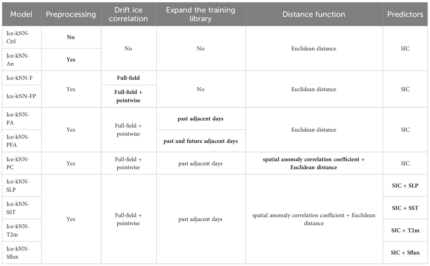
Table 1 Experiment design using the kNN model for the optimization.

FIGURE 1

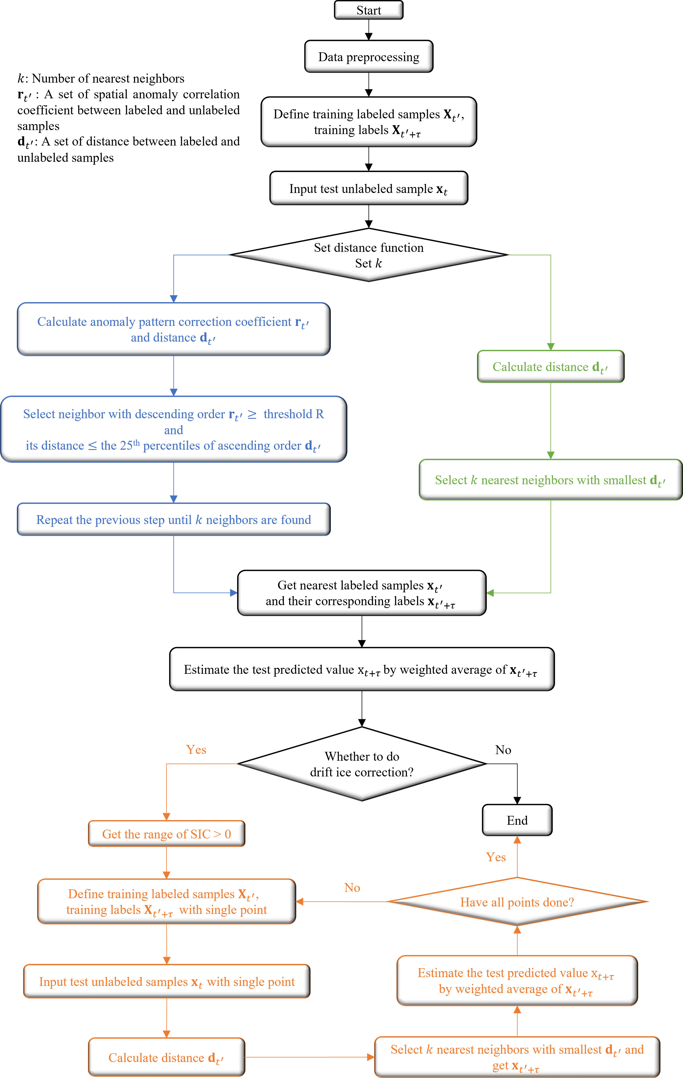
Figure 1 A flowchart showing the processing steps required of using Ice-kNN to predict Arctic sea ice.

All experiments were conducted on the Intel Xeon E5-2609 (1.70GHz, 16 cores). The kNN model does not separate the time of training and prediction, so it needs to go through the training and prediction process all over again with each prediction. One 122-day prediction at an initial time costs about 300 seconds.

3.2.1 Deseasonalization and detrending

Time series forecasting models must address the classical patterns frequently encountered in time series data: trend and seasonality. In contrast to the statistical methodologies, wherein established strategies are used to tackle seasonality, there is no universal agreement among computational intelligence methods for dealing with seasonal patterns. Wang et al. (2016) suggested that the application of detrending may lead to artificial mutation, causing the predicted value of the SIC to exceed the boundary value. Nevertheless, many studies have shown that using anomaly data can achieve better forecast skill (Yuan et al., 2016; Jun Kim et al., 2020; Chi et al., 2021). To determine whether Ice-kNN can benefit from detrending and deseasonalization steps, the Ice-kNN-An experiment was designed, in which the long-term linear trend and the climatological annual cycle of SIC had been subtracted at each grid point.

3.2.2 Drift-ice correlation

Fritzner et al. (2020) indicated that in the kNN model, the modelling of each point is independent of each other, leading to frequent occurrence of drift ice in the Arctic marginal region in the forecast results. Li et al. (2020) proposed a method that considers full-field distance of variables and thus the best similarity type can be found. This method considers the spatial correlation of variables to a certain extent and thus alleviating the drift-ice problem in pointwise prediction. Therefore, this study proposed two drift-ice correlation algorithms: Full_Field (Ice-kNN-F) and Full_Field_Plus_Pointwise (Ice-kNN-FP). In Ice-kNN-F, the sample was defined as the whole pattern of the sea ice concentration anomaly (SICA) rather than single point of SICA. In other words, the features of the sample are expanded. In Ice-kNN-FP, the kNN model first defined the sample as the whole pattern of the SICA to predict the sea ice edge location where SIC greater than 0, and then defined the sample as the grid point of the SICA to predict the SIC within the sea ice edge.

3.2.3 Expand the training library

Owing to the limited length of the SIC satellite record, the training library for each target state has only 32-41 training samples from 2011 to 2020. As in previous studies (Mullan and Thompson, 2006; Li et al., 2020), the past adjacent calendar days are selected in the training library. In this way, the library for each target state was expanded threefold in Ice-kNN_Past_Adjacent_Days (Ice-kNN-PA). In addition, to further verify the sensitivity of predictive skill to the number of samples in training library, the past and future adjacent calendar days (which do not overlap with the forecast period) were selected in the training library in Ice-kNN_Past_Future_Adjacent_Days (Ice-kNN-PFA). A series of preliminary experiments were conducted with varying numbers of adjacent days. These experiments revealed that employing one adjacent day to expand the training library can yield desirable levels of both precision and efficiency (Figure S2). Moderately increasing the training database can effectively make up for the lack of training data, but newly added data may contain noise or irrelevant information. If this data introduces incorrect patterns or inconsistencies, it can lead to larger errors. In addition, time-series data often exhibits strong temporal correlation. In kNN, data points from adjacent dates tend to have more similar features because they may be influenced by similar external factors or trends. However, when you add more adjacent calendar days, the model may not effectively capture this temporal correlation, leading to increased errors.

3.2.4 Distance function

Taking into consideration the spatial continuity of the gridded sea ice data, in Ice-kNN_Pattern_Correlation (Ice- kNN-PC), for a given unlabeled sample x_t, the Euclidean distance and spatial anomaly correlation coefficient were both computed to measure the similarity between samples. The library was then sorted in descending order based on the spatial correlation between fields. The sample with the highest pattern correlation greater than threshold R was selected as the nearest labeled sample, provided that its distance was smaller than the corresponding 25th percentiles of the entire library. If the labeled sample did not satisfy these conditions, the next labeled sample in the list was evaluated. This process was repeated until three nearest labeled samples were identified, if available. If there was no training sample that satisfied these conditions, the training sample with the largest pattern correlation was chosen as the nearest labeled sample. Therefore, it was guaranteed that at least one labeled sample was found. We conducted a preliminary experiment to discuss the impact of different threshold values R on prediction skills. The results show that the prediction skills are best, especially for the lead time less than one month when the threshold R is selected as 0.2 (Figure S3). Therefore, the threshold R of Ice-kNN-PC is set to 0.2.

3.2.5 Predictors

Four ice-related variables that have been frequently used in prior studies (Yuan et al., 2016; Liu et al., 2021), namely SLP, SST, T2m, and Sflux, along with SIC, were chosen to construct the Ice-kNN model. These four experiments are named Ice-kNN-SLP, Ice-kNN-SST, Ice-kNN-T2m, and Ice-kNN-Sflux, respectively.

3.3 Verification metrics

To assess the forecast skill of the experiments, the SIC predictions of the Ice-kNN model were evaluated at each grid cell using the RMSE of SIC (RMSE_SIC) and bias between the prediction and the observations at 1–122 lead days. The bias is the difference between the prediction and observations for the 10-year average from 2011 to 2020. The Arctic is divided into five regions, as shown in Figure S4. Owing to the rapid melting of sea ice in recent years, the grid points where SIC have not changed from 2011 to 2020 were excluded when calculating the regional mean predictive skill (Chi and Kim, 2017; Jun Kim et al., 2020).

For SIE verification, three metrics are used: (1) the error of the September monthly mean SIE (Δ^SIE), (2) the RMSE of SIE (RMSE_SIE), and (3) the integrated ice edge error (IIEE) bias Δ^IIEE (Melsom et al., 2019; Fritzner et al., 2020). The total extent (sum of cell areas where SIC > 15%) for each day in September was computed and then averaged for the month for each year into a September mean SIE. The IIEE bias metric, Δ^IIEE, is a measure of the relative difference in sea ice offset predicted by the model. It is computed from three parts, the overestimated and underestimated local SIE and the length of the ice edge. The overestimated part consists of sea ice-free areas that are predicted to be covered with sea ice, and the underestimated part consists of sea ice-covered areas that are predicted to be sea ice free. The length of the ice edge is determined by the ice edge of the observed and predicted fields. A positive Δ^IIEE bias means that the overestimated SIE in the model is large relative to the underestimated SIE, and vice versa.

Sensitivity tests were conducted with the Ice-kNN model using SIC along with one extra variable as a predictor variable (Jun Kim et al., 2020; Liu et al., 2021). To examine the contribution of each predictor to the predictive skill of SIC, the sensitivity is defined as Sens_SIC; to examine the contribution to the predictive skill of SIE, the sensitivity is defined as Sens_SIE. The sensitivity formulas are as follows:

$\begin{array}{ll}Sens\_SIC\left(predictor\right) =\frac{RMSE\_SI{C}_{sic}-RMSE\_SI{C}_{predictor}}{RMSE\_SI{C}_{sic}} & (2)\end{array}$

$\begin{array}{ll}Sens\_SIE\left(predictor\right) =\frac{RMSE\_SI{E}_{sic}-RMSE\_SI{E}_{predictor}}{RMSE\_SI{E}_{sic}} & (3)\end{array}$

Here RMSE_SIC_sic (RMSE_SIE_sic) is the RMSE_SIC (RMSE_SIE) of forecast using only SIC, and the RMSE_SIC_predictor (RMSE_SIE_predictor) is the RMSE_SIC (RMSE_SIE) of forecast using SIC and one extra predictor.

4 Results

4.1 Impacts of deseasonalization and detrending

To examine whether the data preprocessing strategy for removing the seasonality and trend could improve the forecast accuracy of the Ice-kNN model, the predictive skill of Ice-kNN-An is compared with that of Ice-kNN-Ctrl in this section. Figure 2 shows the comparison of the hindcast skill between Ice-kNN-An and Ice-kNN-Ctrl measured by the different verification metrics. The RMSE_SIC of Ice-kNN-Ctrl increases with the lead time and stays around 16% after one month (Figure 2A). The RMSE_SIC and bias of Ice-kNN-Ctrl in September is mainly distributed in the regions where seasonal sea ice retreats from June to September, including the Beaufort Sea, Chukchi Sea, East Siberian Sea, and Laptev Sea, and it is higher than the climatological prediction in all studied areas (Figures 3, 4A). For SIE, the RMSE_SIE of Ice-kNN-Ctrl increases with lead time and reaches 2.2 × 10⁶ km² in September (Figure 2B). Compared with the observations, the prediction of Ice-kNN-Ctrl always overestimates SIE from June to September, and the overestimation gradually increases with the retreat of seasonal sea ice (Figures 2C, S5A). It may be related to the difficulty of marginal sea ice prediction and the prediction bias of the Ice-kNN model with the increasing prediction time (Guemas et al., 2016; Liu et al., 2021).

FIGURE 2

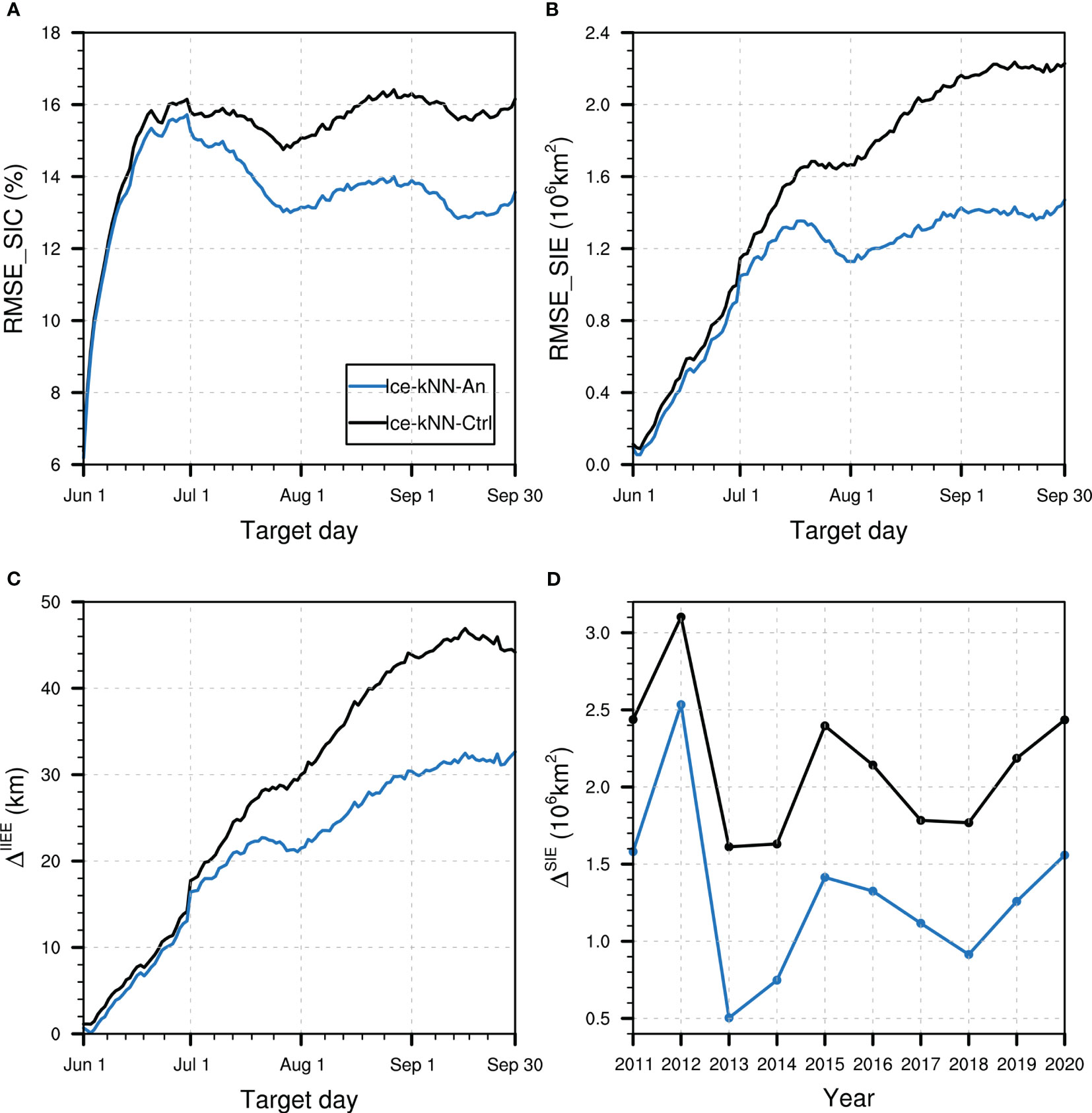
Figure 2 Hindcast skill comparison between Ice-kNN-Ctrl (black) and Ice-kNN-An (blue) measured by (A) spatial averaged RMSE_SIC, (B) RMSE_SIE, (C) ${\Delta }^{\text{IIEE}}$, and (D) ${\Delta }^{\text{SIE}}$.

FIGURE 3

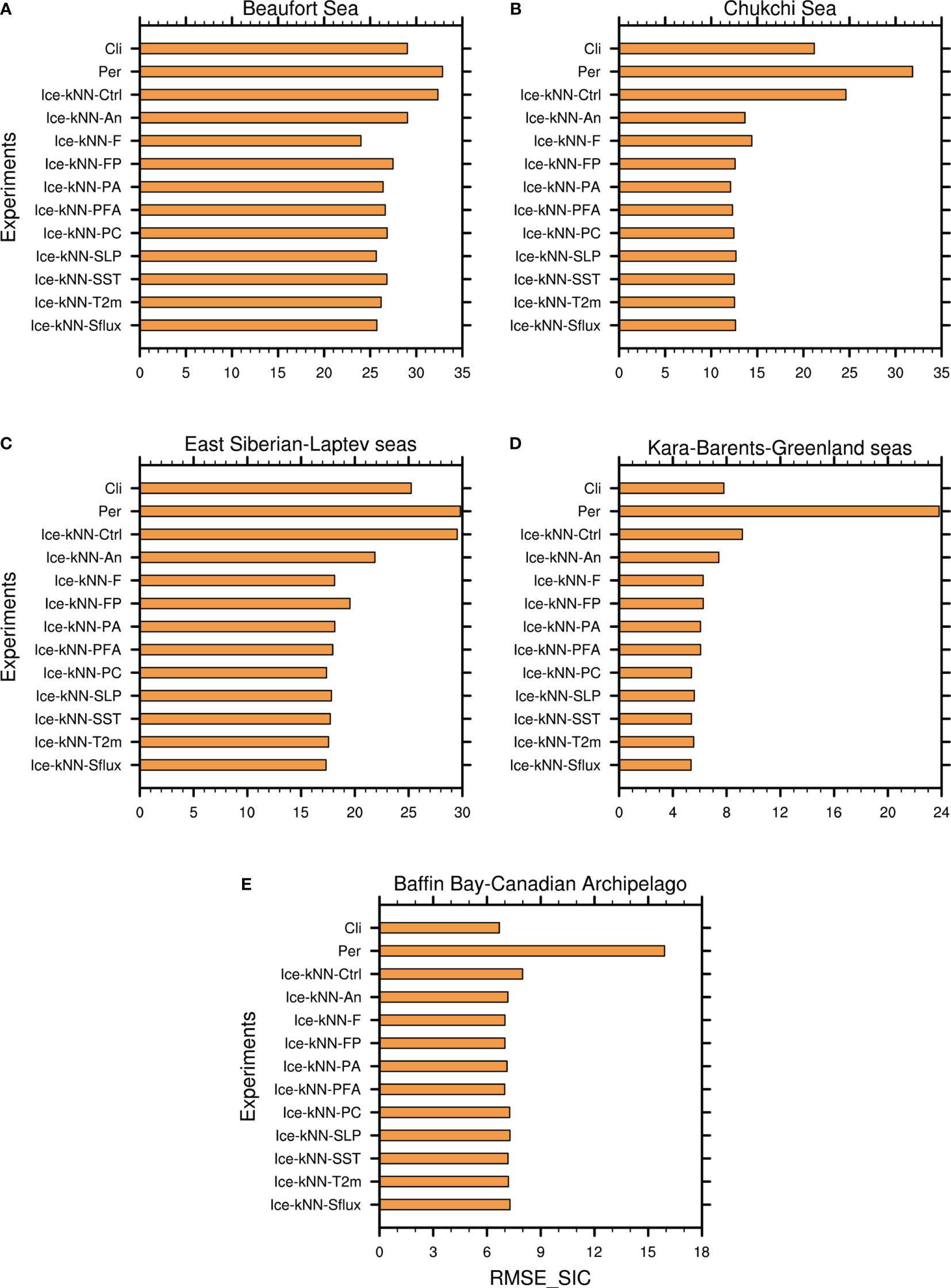
Figure 3 Spatial averaged RMSE_SIC of the Ice-kNN model in hindcasting September SIC averaged from 2011 to 2020 in the (A) Beaufort Sea, (B) Chukchi Sea, (C) East Siberian–Laptev seas, (D) Kara–Barents-Greenland seas, and (E) Baffin Bay–Canadian Archipelago.

FIGURE 4

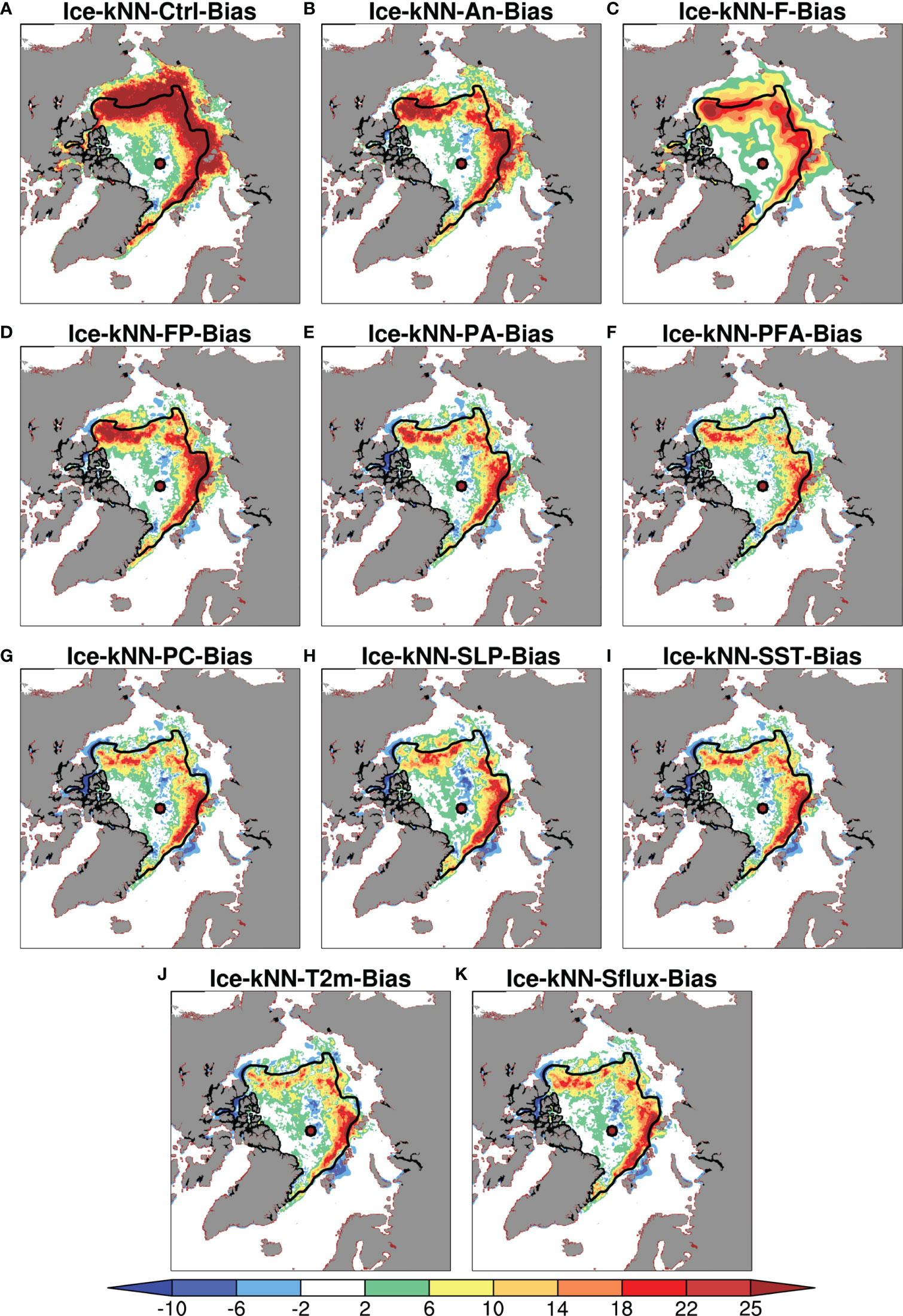
Figure 4 The prediction bias between the Ice-kNN model and the observation of (A) Ice-kNN-Ctrl-Bias, (B) Ice-kNN-An-Bias, (C) Ice-kNN-F-Bias, (D) Ice-kNN-FP-Bias, (E) Ice-kNN-PA-Bias, (F) Ice-kNN-PFA-Bias, (G) Ice-kNN-PC-Bias, (H) Ice-kNN-SLP-Bias, (I) Ice-kNN-SST-Bias, (J) Ice-kNN-T2m-Bias, and (K) Ice-kNN-Sflux-Bias in September averaged from 2011 to 2020. The black line represents the outline of the 10-year (2011-2020) mean extent for the September.

For Ice-kNN-An, there is notable skill enhancement in predicting SIC at lead times longer than one month, and the enhancement of Ice-kNN-An is more pronounced with lead time (Figure 2A). According to the spatial pattern, the September RMSE_SIC and bias of Ice-kNN-An in all areas is lower compared with Ice-kNN-Ctrl (Figures 3, 4A, B). For SIE, although both Ice-kNN-An and Ice-kNN-Ctrl tend to overestimate SIE in summer, the predictive skill of Ice-kNN-An is significantly superior than that of Ice-kNN-Ctrl for summer SIE and the improvement increases with lead time (Figure 2C). This indicates that the Ice-kNN model can better find the temporal evolution of sea ice by extracting the seasonality and trend, especially from an ice-covered period to an ice-free period.

In extreme ice cover years, such as record low in 2012, the forecast biases are relatively large compared to other years for both models (Figure 2D). On the one hand, the lowest minimum Arctic SIE in 2012 is associated with the large multiyear ice volume export and the storm that entered into the central Arctic in early August 2012 (Parkinson & Comiso, 2013; Li et al., 2022). Since the initial day is fixed on June 1st, it is hard for Ice-kNN model to catch the atmospheric disturbance in the extreme cases. On the other hand, for the extreme cases of SIE, Ice-kNN model is not suitable to forecast the extreme values which are not included in the training library due to its prediction principle. While in the other years, Ice-kNN-An shows an impressive improvement compared with Ice-kNN-Ctrl (Figure 2D). However, there is still considerable drift ice outside the sea ice edge in both experiments (Figures S5A, B).

The improvement of Ice-kNN-An indicates that the deseasonalization and detrending step is useful to improve the Arctic sea ice forecast accuracy of the Ice-kNN model. Therefore, the data preprocessing strategy was used to remove the seasonality and the trend components in subsequent experiments.

4.2 Impact of drift-ice correlation

Due to the lack of spatial continuity in the traditional kNN model, both Ice-kNN-Ctrl and Ice-kNN-An forecasts showed unrealistic drift ice around the sea ice edge (Figures S5A, B). This section studies the impact of different drift-ice correction algorithms in the Ice-kNN prediction. As shown in Figure 5A, the RMSE_SIC of Ice-kNN-F shows poor predictive skill at lead times of less than 30 days, but it is better than Ice-kNN-An at lead times longer than 30 days. According to the distribution of September RMSE_SIC and bias, Ice-kNN-F is superior to Ice-kNN-An in predicting SIC in September in all sea areas except the Chukchi Sea (Figures 3, 4B, C). The results show that the pointwise modeling is better for the prediction of SICA caused by short-term-scale disturbances, whereas for the SICA caused by large-scale anomalies, selecting the similarity using the full-field distance could improve the predictive skill with lead times of more than one month. Ice-kNN-FP predicted the SIC point by point based on Ice-kNN-F determination of the sea ice edge. It performs better than Ice-kNN-F at lead times of less than 30 days and better than Ice-kNN-An at lead times of longer than 30 days (Figure 5A). In addition, Ice-kNN-FP has a lower unrealistic drift-ice bias compared with Ice-kNN-An, especially in the Chukchi, East Siberian, Laptev, and Kara seas (Figures 3, S5B, D).

FIGURE 5

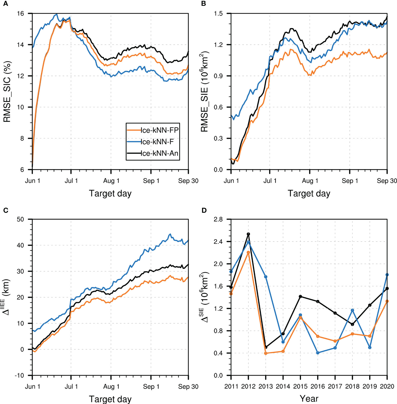
Figure 5 Hindcast skill comparison between Ice-kNN-An (black), Ice-kNN-F (blue), and Ice-kNN-FP (orange) measured by (A) spatial averaged RMSE_SIC, (B) RMSE_SIE, (C) Δ^IIEE, and (D) Δ^SIE.

For SIE, the prediction bias of Ice-kNN-F in the short-term lead time is larger. However, Ice-kNN-FP, which combines full-field distance and single-point distance, shows a significant improvement in sea ice edge compared with Ice-kNN-F and Ice-kNN-An for the whole lead time (Figures 5B, C). In Figure 5D, it can be seen that Ice-kNN-FP effectively reduces the bias of the September mean SIE in Ice-kNN-F and Ice-kNN-An in most years.

The kNN model, which takes only a single grid point as the prediction sample, lacks physical spatial connection, and leads to the prediction of unrealistic drift ice. A drift-ice correlation algorithm, which selects similarity by full-field distance, would consider the spatial continuity of sea ice but ignore the local SICA caused by short-term disturbance. Therefore, the full-field distance is first used to limit the sea ice coverage, and then pointwise modelling is carried out to predict the SIC of each single grid point, which can effectively correct the unrealistic drift ice of pointwise modelling and the initial sea ice migration bias of full-field modelling. In the following kNN models, the drift-ice correction algorithm of Ice-kNN-FP is applied.

4.3 Impact of expanding the training library

In principle, the nearest neighbors with insufficient similarity could diverge relatively quickly in time compared with the very close nearest neighbors. The limited Ice-kNN forecast skill may therefore be partly due to the relatively small number of available training labeled samples, which makes the nearest neighbor selection a challenge. As the most accurate summer SIC datasets are limited to the satellite era starting in the 1979, the training labeled samples for each state has only 32 to 41 members from 2011 to 2020. To verify the sensitivity of the predictive skill to the number of training labeled samples, Ice-kNN-PA and Ice-kNN-PFA expand the training library by adding adjacent calendar days. The number of training labels samples in Ice-kNN-PA increases from 96 to 123 from 2011 to 2020, and that in Ice-kNN-PFA increases to 123.

Compared with Ice-kNN-FP, the RMSE_SICs of the Ice-kNN-PA and Ice-kNN-PFA seems not to be significantly reduced (Figure 6A), but from the perspective of different sea areas, the Ice-kNN-PA and Ice-kNN-PFA mainly reduced the positive SIC bias in the sea ice marginal zone of Beaufort Sea and the East SiberianLaptev seas (Figures 4D–F, S6A, B). For SIE, Ice-kNN-PA and Ice-kNN-PFA have a larger initial bias at lead times of less than two weeks (Figure 6B), which is mainly due to the underestimation of SIE (Figure 6C). However, Ice-kNN-PA and Ice-kNN-PFA show significant improvement in predicting SIE after that (Figures 6B, C). In Figure 6D, except for 2017 in Ice-kNN-PFA, the September mean SIE bias of Ice-kNN-PA and Ice-kNN-PFA is reduced by about 0.5 million square kilometers compared with Ice-kNN-FP.

FIGURE 6

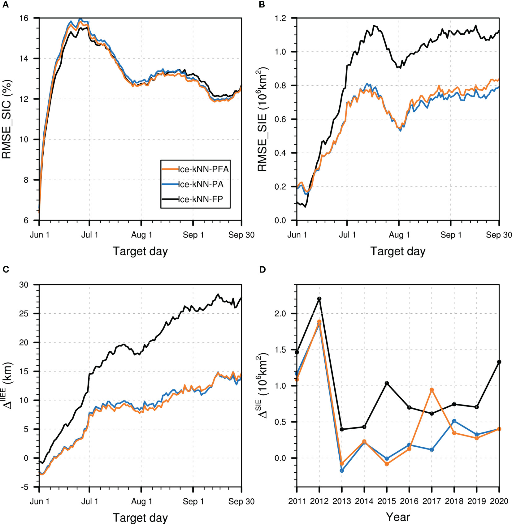
Figure 6 Hindcast skill comparison between Ice-kNN-FP (black), Ice-kNN-PA (blue), and Ice-kNN-PFA (orange) measured by (A) spatial averaged RMSE_SIC, (B) RMSE_SIE, (C) Δ^IIEE, and (D) Δ^SIE.

In general, expanding the training library will cause an initial underestimation bias, but it will not rapidly diverge with increasing lead time. The predictive skill of the experiments that use the expanded training library are significantly improved compared with Ice-kNN-FP with lead times of more than two weeks. Using the future adjacent calendar days as the training labeled samples has relatively little impact, except for 2017 when Ice-kNN-PFA selects future sample as the nearest sample. The younger and thinner Arctic sea ice in recent years is more sensitive to external forcing (Parkinson & Comiso, 2013), resulting in a large deviation in the forecast results when the future adjacent calendar days are selected in the training library.

Therefore, selecting sufficient training labeled samples could better improve the predictive skill of the Ice-kNN model for Arctic sea ice. In subsequent experiments, the strategy of expanding the training library by adding past adjacent calendar days as training labeled samples to predict the Arctic sea ice was applied.

4.4 Impact of distance function

In previous Ice-kNN models, the Euclidean distance has been selected most frequently as the distance function. In the prediction of sea ice, not only the distance between grid cells but also the spatial correlation coefficient between states should be considered to select similarity. In this section, a compound distance function scheme, including the spatial anomaly correlation coefficient and the Euclidean distance between sea ice, is studied.

As shown in Figure 7A, the RMSE_SIC of Ice-kNN-PC is comparable to that of Ice-kNN-PA. According to the spatial pattern, the September RMSE_SIC and bias of Ice-kNN-PC decreases in the East Siberian–Laptev seas and Kara–Barents–Greenland seas, but increases in the Beaufort Sea, Chukchi Sea, and Baffin Bay–Canadian Archipelago compared with Ice-kNN-PA (Figures 3, 4F, G). For the SIE, the RMSE_SIE of Ice-kNN-PC has a larger bias at lead times of less than one week (Figure 7B), which is mainly due to the underestimation of SIE (Figure 7C). However, Ice-kNN-PC shows improvement in SIE compared with Ice-kNN-PA at lead times of more than one week and the improvement is more pronounced with increasing lead time (Figures 7B, C). In the Figure 7D, except for 2012, the biases of monthly mean SIE in September of Ice-kNN-PC from 2011 to 2020 are within about 0.5 million square kilometers, which is lower than Ice-kNN-PA.

FIGURE 7

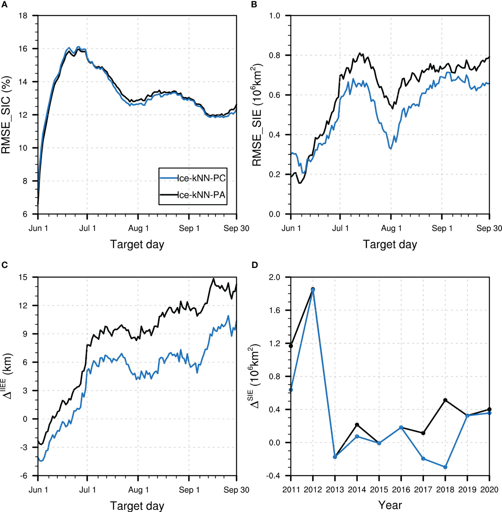
Figure 7 Hindcast skill comparison between Ice-kNN-PA (black) and Ice-kNN-PC (blue) measured by (A) spatial averaged RMSE_SIC, (B) RMSE_SIE, (C) Δ^IIEE, and (D) Δ^SIE.

In general, the composite distance function with a spatial anomaly correlation coefficient is beneficial to the prediction of Arctic sea ice. The new distance function considers not only the similarity between samples at a single point through the Euclidean distance but also the spatial mode of the SICA through the spatial anomaly correlation coefficient. It is helpful for the Ice-kNN model to consider the large-scale spatial variation of SICA when selecting the similarity. Therefore, in the following experiments, a composite distance function combining the Euclidean distance and the spatial anomaly correlation coefficient is used to further improve the predictive skill of the Ice-kNN model.

4.5 Impact of sea ice-related predictors

To verify the impact of sea ice-related atmospheric and oceanic variables on the predictive skill of summer Arctic sea ice, SIC and SIE sensitivity indices including sea ice-related variables were calculated based on the Ice-kNN-PC model in Figure 8. A positive sensitivity index indicates that a variable has a positive contribution to the predictive skill of SIC (SIE).

FIGURE 8

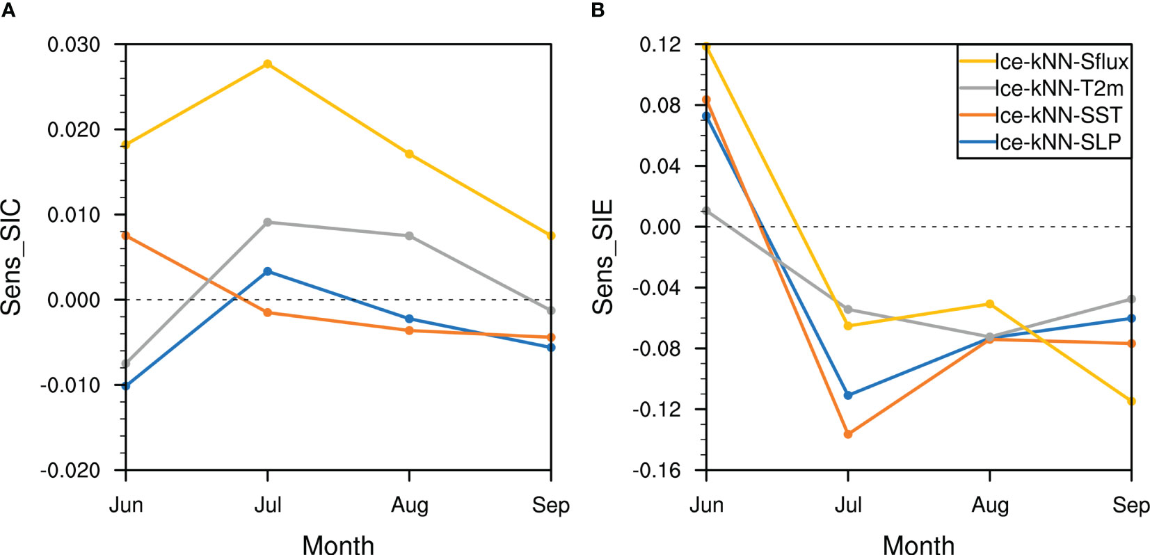
Figure 8 The monthly mean sensitivity indexes from June to September of (A) RMSE_SIC-based for SIC and (B) RMSE_SIE-based for SIE with kNN using different predictors (blue, SIC/SLP; orange, SIC/SST; grey, SIC/T2m; yellow, SIC/Sflux).

Ice-kNN-Sflux, which selects Sflux and SIC as predictors, improves the predictive skill of SIC for the whole lead time (Figure 8A). SST improves the predictive skill at lead times of less than one month, but SLP and T2m provide only limited improvement in the predictive skill at lead times of about one to two months (Figure 8A). According to the distribution of RMSE_SIC and bias in September, the improvement of the predictive skill of Ice-kNN-Sflux mainly occurs in the Beaufort Sea, compared with Ice-kNN-PC (Figures 3A, 4G–K). For SIE, the sensitivity index is calculated based on the RMSE_SIE. All the sea ice-related variables show improvement of the SIE predictive skill at lead times of less than one month. But for lead times longer than one month, all the sea ice-related variables show negative contributions to the predictive skill of SIE.

The predictive skill of Ice-kNN-Sflux for SIC is significantly better than both the climatological prediction and the anomaly persistence prediction at lead times of longer than two weeks (Figure S7). The predictive skill of Ice-kNN-Sflux for September SIC is significantly better than the anomaly persistence prediction for the whole Arctic, and significantly better than the climatological prediction for the whole Arctic, except for Baffin Bay and the Canadian Islands (Figure 3). The prediction bias of Ice-kNN-Sflux in September SIE is reduced by 2.0 × 10⁶ km² compared with the climatological prediction and by 3.0 × 10⁶ km² compared with the anomaly persistence prediction.

In general, for daily Arctic sea ice forecasts in summer, the Sflux fields, which have a direct relation to sea ice (Liu et al., 2021), can enhance the predictive skill of sea ice. SLP and T2m show little improvement of the predictive skill of sea ice, which may result from the chaotic behavior of the atmosphere (Mohammadi-Aragh et al., 2018). While the surface oceanic field SST does not show its long-term memory, which may result from the interpolation bias. Similar results were obtained in Liu et al. (2021) using the deep learning model ConvLSTM.

4.6 Comparison of SIE

The Sea Ice Prediction Network (SIPN) is an open platform that has been collecting predictions of Arctic SIE in September around the world since 2008, then compiling and presenting them to those interested in Arctic sea ice. September SIE predictions have been submitted to the SIPN in June, July, and August since 2008, with an additional September submission added in 2021. There are a variety of prediction methods, including heuristic, statistical, mixed, dynamic, and machine learning/other. To further evaluate the Arctic sea ice forecast skill of Ice-kNN model, we compared the Arctic September SIEs in 2021 and 2022 using the Ice-kNN-Sflux model with the observations and the contributions for the September SIE predictions to the Post-Season Sea Ice Outlook for 2021 and 2022 (Bhatt et al., 2022a; Bhatt et al., 2022b). We utilized the SIC of May 31, June 30, July 31 and August 31 respectively as the input of Ice-kNN-Sflux model to predict the September SIEs. It should be noted here we use a hindcast (not real-time forecast) result of the Ice-kNN-Sflux model.

As shown in Figure 9A, the observed September SIE in 2021 was 4.92 × 10⁶ km² (reported by NSIDC). The median hindcasting result of Ice-kNN-Sflux from June to September is 4.8 × 10⁶ km², with a quartile range of 4.62 to 5.04 × 10⁶ km² (Figure 9A). The median September estimate based on all contributors of SIPN were 4.37 × 10⁶, 4.36 × 10⁶, 4.39 × 10⁶, and 4.39 × 10⁶ km², respectively, from June to September. In comparison, our hindcasts using Ice-kNN-Sflux were 5.34 × 10⁶, 4.94 × 10⁶, 4.66 × 10⁶, and 4.49 × 10⁶ km², respectively (Table S1A). For 2022, the medians September estimate of SIPN were 4.57 × 10⁶, 4.64 × 10⁶, 4.83 × 10⁶, and 4.91 × 10⁶ km², respectively, from June to September, which approaches observation 4.87 × 10⁶ km² (reported by the NSIDC). The hindcasts of Ice-kNN-Sflux from June to September were 5.05 × 10⁶, 4.47 × 10⁶, 5.65 × 10⁶, and 4.62 × 10⁶ km² (Table S1B). The median hindcasting result of Ice-kNN-Sflux from June to September is 4.835 × 10⁶ km², with a quartile range of 4.58 to 5.2 × 10⁶ km² (Figure 9B).

FIGURE 9

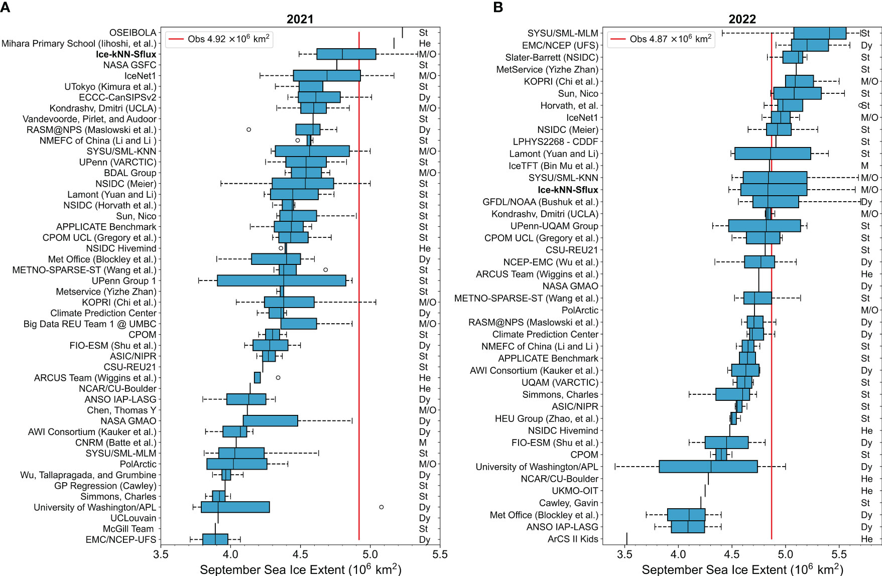
Figure 9 The SIPN forecast box plots for the estimates of September Arctic SIE in (A) 2021 and (B) 2022 by ML/Other (M/O), Mixed (M), Dynamic (Dy), Statistical (St) and Heuristic (He). Our model hindcasts of Ice-kNN-Sflux has been bolded. The data for this Figure were adapted from the Sea Ice Prediction Network.

5 Conclusions and discussion

In this study, a SIC dataset of remote sensing was utilized and a machine learning model, Ice-kNN, has been introduced and optimized to improve the prediction skill of summer Arctic SIC for a 122-day prediction. The results show that when the traditional kNN model is directly applied to predict the summer Arctic SIC, its September predictive skill is poorer than the climatological prediction for the whole Arctic, which is due to the inability of the kNN model to identify the seasonal variability of SIC in summer Arctic. To address this issue, we proposed different processes to improve the performance of the Ice-kNN model, including the data preprocessing of deseasonalization and detrending, a drift-ice correction algorithm, expansion of the training library, a distance function, and predictors. By using these algorithms, we aimed to optimize the results of the Ice-kNN model. Our sensitivity analysis revealed that the seasonalization and trends of the data need to be preprocessed to improve the identification of sea ice variability by the Ice-kNN model. Although the traditional kNN model has no spatial relation, the sea ice coverage can be constrained by defining the samples as a pattern of SICA and using the composite distance function combined with a spatial anomaly correlation coefficient and Euclidean distance. In addition, selecting sufficient training labeled samples improves the predictive skill of the Ice-kNN model for Arctic sea ice. Besides, the importance of sea ice-related variables was studied through sensitivity tests. The introduction of Sflux into the Ice-kNN model effectively improved the predictive skill of the model, whereas the addition of SLP, T2m, and SST did not significantly improve the predictive skill.

The Ice-kNN-Sflux model was evaluated against climatological and anomaly persistence predictions. There is notable skill enhancement in the hindcasts of Arctic sea ice using the Ice-kNN-Sflux model, which is more pronounced with increasing lead time. The September mean SIE of the Ice-kNN-Sflux hindcasts was reduced by about 2.0 × 10⁶ km² and 3.0 × 10⁶ km² compared with the climatological and the anomaly persistence predictions. In addition, the September SIE was found to be reasonably well predicted compared with the forecasts submitted to the SIPN in 2021 and 2022. Overall, our study provides important insights into predicting summer daily Arctic SIC and highlights the potential benefits of using modified Ice-kNN for this purpose.

Although this Ice-kNN model shows great potential for summer daily Arctic sea ice prediction, more experiments need to be conducted to improve the Ice-kNN model and examine its robustness. Future studies are needed to further expand the initial forecast days of the Ice-kNN model. In addition, the combined effects of the predictors mentioned in this study on the Ice-kNN model are not considered and Arctic SIC is also influenced by a variety of other factors, such as ice drift, surface albedo and ocean heat content (Shimada et al., 2006; Screen and Simmonds, 2010; Mahajan et al., 2011; Liu et al., 2021). Therefore, it is necessary to study different combinations of predictors and include more predictor variables related to sea ice for feature processing to strengthen the understanding of the multivariable processes.

Data availability statement

The original contributions presented in the study are included in the article/Supplementary Material. Further inquiries can be directed to the corresponding author.

Author contributions

YL: Conceptualization, Data curation, Formal Analysis, Investigation, Methodology, Software, Validation, Visualization, Writing – original draft, Writing – review and editing. QY: Conceptualization, Funding acquisition, Project administration, Resources, Supervision, Writing – review and editing. XL: Conceptualization, Investigation, Methodology, Resources, Supervision, Validation, Writing – review and editing. CY: Conceptualization, Supervision, Writing – review and editing. YW: Writing – review and editing, Supervision. JW: Writing – review and editing, Supervision. JinL: Writing – review and editing, Conceptualization, Data curation, Investigation. SC: Writing – review and editing, Data curation, Investigation. JipL: Supervision, Writing – review and editing.

Funding

The author(s) declare financial support was received for the research, authorship, and/or publication of this article. This work was supported by the Southern Marine Science and Engineering Guangdong Laboratory (Zhuhai) (NO. SML2020sp007), the Guangdong Basic and Applied Basic Research Foundation (No. 2020B1515020025), the National Key R&D Program of China (No. 2022YFE0106300), the National Natural Science Foundation of China (No. 42106233, 42106226, 41922044) and the fundamental research funds for the Norges Forskningsråd (No. 328886).

Conflict of interest

The authors declare that the research was conducted in the absence of any commercial or financial relationships that could be construed as a potential conflict of interest.

Publisher’s note

All claims expressed in this article are solely those of the authors and do not necessarily represent those of their affiliated organizations, or those of the publisher, the editors and the reviewers. Any product that may be evaluated in this article, or claim that may be made by its manufacturer, is not guaranteed or endorsed by the publisher.

Supplementary material

The Supplementary Material for this article can be found online at: https://www.frontiersin.org/articles/10.3389/fmars.2023.1260047/full#supplementary-material

References

Andersson T. R., Hosking J. S., Pérez-Ortiz M., Paige B., Elliott A., Russell C., et al. (2021). Seasonal Arctic sea ice forecasting with probabilistic deep learning. Nat. Commun. 12 (1), 1–12. doi: 10.1038/s41467-021-25257-4

PubMed Abstract | CrossRef Full Text | Google Scholar

Bhatt U. S., Bieniek P., Bitz C. M., Blanchard-Wrigglesworth E., Eicken H., Fisher H. M., et al. (2022a) 2021 sea ice outlook post-season report. Available at: https://www.arcus.org/sipn/sea-ice-outlook/2021/post-season.

Google Scholar

Bhatt U. S., Meier W., Blanchard-Wrigglesworth E., Massonnet F., Goessling H., Ludwig V., et al. (2022b) Sea ice outlook: 2022 post season report. Available at: https://www.arcus.org/sipn/sea-ice-outlook/2022/post-season.

Google Scholar

Chen J., Kang S., Chen C., You Q., Du W., Xu M., et al. (2020). Changes in sea ice and future accessibility along the Arctic Northeast Passage. Glob. Planet. Change 195, 103319. doi: 10.1016/j.gloplacha.2020.103319

CrossRef Full Text | Google Scholar

Chi J., Bae J., Kwon Y. J. (2021). Two-stream convolutional long-and short-term memory model using perceptual loss for sequence-to-sequence arctic sea ice prediction. Remote Sens. 13 (17), 3413. doi: 10.3390/rs13173413

CrossRef Full Text | Google Scholar

Chi J., Kim H. C. (2017). Prediction of Arctic sea ice concentration using a fully data driven deep neural network. Remote Sens. 9 (12), 1305. doi: 10.3390/rs9121305

CrossRef Full Text | Google Scholar

Deng Z., Zhu X., Cheng D., Zong M., Zhang S. (2016). Efficient kNN classification algorithm for big data. Neurocomputing 195, 143–148. doi: 10.1016/j.neucom.2015.08.112

CrossRef Full Text | Google Scholar

Fritzner S., Graversen R., Christensen K. H. (2020). Assessment of high-resolution dynamical and machine learning models for prediction of sea ice concentration in a regional application. J. Geophys. Res. Ocean. 125 (11), 1–23. doi: 10.1029/2020JC016277

CrossRef Full Text | Google Scholar

Guemas V., Blanchard-Wrigglesworth E., Chevallier M., Day J. J., Déqué M., Doblas-Reyes F. J., et al. (2016). A review on Arctic sea-ice predictability and prediction on seasonal to decadal time-scales. Q. J. R. Meteorol. Soc 142 (695), 546–561. doi: 10.1002/qj.2401

CrossRef Full Text | Google Scholar

Hersbach H., Bell B., Berrisford P., Hirahara S., Horányi A., Muñoz Sabater J., et al. (2020). The ERA5 global reanalysis. Q. J. R. Meteorolog. Soc. 146 (730), , 1999–2049. doi: 10.1002/qj.3803

CrossRef Full Text | Google Scholar

Huang B., Liu C., Banzon V., Freeman E., Graham G., Hankins B., et al. (2021). Improvements of the daily optimum interpolation sea surface temperature (DOISST) version 2.1. J. Clim. 34 (8), 2923–2939. doi: 10.1175/JCLI-D-20-0166.1

CrossRef Full Text | Google Scholar

Jun Kim Y., Kim H. C., Han D., Lee S., Im J. (2020). Prediction of monthly Arctic sea ice concentrations using satellite and reanalysis data based on convolutional neural networks. Cryosphere 14 (3), 1083–1104. doi: 10.5194/tc-14-1083-2020

CrossRef Full Text | Google Scholar

Kwok R. (2018). Arctic sea ice thickness, volume, and multiyear ice coverage: Losses and coupled variability, (1958-2018). Environ. Res. Lett. 13 (10). doi: 10.1088/1748-9326/aae3ec

CrossRef Full Text | Google Scholar

Li X., Bordbar M. H., Latif M., Park W., Harlaß J. (2020). Monthly to seasonal prediction of tropical Atlantic sea surface temperature with statistical models constructed from observations and data from the Kiel Climate Model. Clim. Dyn. 54 (3–4), 1829–1850. doi: 10.1007/s00382-020-05140-6

CrossRef Full Text | Google Scholar

Li X., Yang Q., Yu L., Holland P. R., Min C., Mu L., et al. (2022). Unprecedented Arctic sea ice thickness loss and multiyear-ice volume export through Fram Strait during 2010-2011. Environ. Res. Lett. 17 (9), 095008. doi: 10.1088/1748-9326/ac8be7

CrossRef Full Text | Google Scholar

Lindsay R. W., Zhang J., Schweiger A. J., Steele M. A. (2008). Seasonal predictions of ice extent in the Arctic Ocean. J. Geophys. Res. Ocean. 113 (2), 1–11. doi: 10.1029/2007JC004259

CrossRef Full Text | Google Scholar

Liu Y., Bogaardt L., Attema J., Hazeleger W. (2021). Extended-range arctic sea ice forecast with convolutional long short-Term memory networks. Mon. Weather Rev. 149 (6), 1673–1693. doi: 10.1175/MWR-D-20-0113.1

CrossRef Full Text | Google Scholar

Mahajan S., Zhang R., Delworth T. L. (2011). Impact of the atlantic meridional overturning circulation (AMOC) on arctic surface air temperature and sea ice variability. J. Clim. 24 (24), 6573–6581. doi: 10.1175/2011JCLI4002.1

CrossRef Full Text | Google Scholar

Maslanik J., Stroeve J. (1999). “Near-Real-Time DMSP SSMIS Daily Polar Gridded Sea Ice Concentrations, Version 1.” NASA Nat. Snow Ice Data Center Distrib. Act. Arch. Center. doi: 10.5067/U8C09DWVX9LM

CrossRef Full Text | Google Scholar

Melia N., Haines K., Hawkins E. (2016). Sea ice decline and 21st century trans-Arctic shipping routes. Geophys. Res. Lett. 43 (18), 9720–9728. doi: 10.1002/2016GL069315

CrossRef Full Text | Google Scholar

Melsom A., Palerme C., Müller M. (2019). Validation metrics for ice edge position forecasts. Ocean Sci. 15 (3), 615–630. doi: 10.5194/os-15-615-2019

CrossRef Full Text | Google Scholar

Min C., Yang Q., Chen D., Yang Y., Zhou X., Shu Q., et al. (2022). The emerging arctic shipping corridors. Geophys. Res. Lett. 49 (10), 1–10. doi: 10.1029/2022GL099157

PubMed Abstract | CrossRef Full Text | Google Scholar

Mohammadi-Aragh M., Goessling H. F., Losch M., Hutter N., Jung T. (2018). Predictability of Arctic sea ice on weather time scales. Sci. Rep. 8 (1), 1–7. doi: 10.1038/s41598-018-24660-0

PubMed Abstract | CrossRef Full Text | Google Scholar

Mu B., Luo X., Yuan S., Liang X. (2023) IceTFT v 1 . 0 . 0 : interpretable long-term prediction of arctic sea ice extent with deep learning (Accessed January, 1–28).

Google Scholar

Mullan A. B., Thompson C. S. (2006). Analogue forecasting of New Zealand climate anomalies. Int. J. Climatol. 26 (4), 485–504. doi: 10.1002/joc.1261

CrossRef Full Text | Google Scholar

Parkinson C. L., Comiso J. C. (2013). On the 2012 record low Arctic sea ice cover: Combined impact of preconditioning and an August storm. Geophys. Res. Lett. 40 (7), 1356–1361. doi: 10.1002/grl.50349

CrossRef Full Text | Google Scholar

Post E., Bhatt U. S., Bitz C. M., Brodie J. F., Fulton T. L., Hebblewhite M., et al. (2013). Ecological consequences of sea-ice decline. Science 341 (6145), 519–524. doi: 10.1126/science.1235225

PubMed Abstract | CrossRef Full Text | Google Scholar

Reichstein M., Camps-Valls G., Stevens B., Jung M., Denzler J., Carvalhais N., et al. (2019). Deep learning and process understanding for data-driven Earth system science. Nature 566 (7743), 195–204. doi: 10.1038/s41586-019-0912-1

PubMed Abstract | CrossRef Full Text | Google Scholar

Screen J. A., Simmonds I. (2010). The central role of diminishing sea ice in recent Arctic temperature amplification. Nature 464 (7293), 1334–1337. doi: 10.1038/nature09051

PubMed Abstract | CrossRef Full Text | Google Scholar

Serreze M. C., Meier W. N. (2019). The Arctic’s sea ice cover: trends, variability, predictability, and comparisons to the Antarctic. Ann. N. Y. Acad. Sci. 1436 (1), 36–53. doi: 10.1111/nyas.13856

PubMed Abstract | CrossRef Full Text | Google Scholar

Shimada K., Kamoshida T., Itoh M., Nishino S., Carmack E., McLaughlin F., et al. (2006). Pacific Ocean inflow: Influence on catastrophic reduction of sea ice cover in the Arctic Ocean. Geophys. Res. Lett. 33 (8), 3–6. doi: 10.1029/2005GL025624

CrossRef Full Text | Google Scholar

Steele M., Ermold W., Zhang J. (2008). Arctic Ocean surface warming trends over the past 100 years. Geophys. Res. Lett. 35 (2), 1–6. doi: 10.1029/2007GL031651

CrossRef Full Text | Google Scholar

Stroeve J., Notz D. (2018). Changing state of Arctic sea ice across all seasons. Environ. Res. Lett. 13 (10), 103001. doi: 10.1088/1748-9326/aade56

CrossRef Full Text | Google Scholar

Stroeve J. C., Serreze M. C., Holland M. M., Kay J. E., Malanik J., Barrett A. P. (2012). The Arctic’s rapidly shrinking sea ice cover: A research synthesis. Clim. Change 110 (3–4), 1005–1027. doi: 10.1007/s10584-011-0101-1

CrossRef Full Text | Google Scholar

Thanh Noi P., Kappas M. (2017). Comparison of random forest, k-nearest neighbor, and support vector machine classifiers for land cover classification using sentinel-2 imagery. Sensors 18 (1), 18. doi: 10.3390/s18010018

PubMed Abstract | CrossRef Full Text | Google Scholar

Vihma T. (2014). Effects of arctic sea ice decline on weather and climate: A review. Surv. Geophys. 35 (5), 1175–1214. doi: 10.1007/s10712-014-9284-0

CrossRef Full Text | Google Scholar

Wang L., Yuan X., Li C. (2019). Subseasonal forecast of Arctic sea ice concentration via statistical approaches. Clim. Dyn. 52 (7–8), 4953–4971. doi: 10.1007/s00382-018-4426-6

CrossRef Full Text | Google Scholar

Wang L., Yuan X., Ting M., Li C. (2016). Predicting summer arctic sea ice concentration intraseasonal variability using a vector autoregressive model. J. Clim. 29 (4), 1529–1543. doi: 10.1175/JCLI-D-15-0313.1

CrossRef Full Text | Google Scholar

Wei K., Liu J., Bao Q., He B., Ma J., Li M., et al. (2021). Subseasonal to seasonal Arctic sea-ice prediction: A grand challenge of climate science. Atmos. Ocean. Sci. Lett. 14 (4), 100052. doi: 10.1016/j.aosl.2021.100052

CrossRef Full Text | Google Scholar

Yang C. Y., Liu J., Xu S. (2020). Seasonal arctic sea ice prediction using a newly developed fully coupled regional model with the assimilation of satellite sea ice observations. J. Adv. Model. Earth Syst. 12 (5), 1–25. doi: 10.1029/2019MS001938

CrossRef Full Text | Google Scholar

Yuan X., Chen D., Li C., Wang L., Wang W. (2016). Arctic sea ice seasonal prediction by a linear Markov model. J. Clim. 29 (22), 8151–8173. doi: 10.1175/JCLI-D-15-0858.1

CrossRef Full Text | Google Scholar

Zhang S., Li X., Zong M., Zhu X., Cheng D. (2017). Learning k for kNN Classification. ACM Trans. Intell. Syst. Technol. 8 (3), 43. doi: 10.1145/2990508

CrossRef Full Text | Google Scholar

Zhang S., Li X., Zong M., Zhu X., Wang R., Zhang S., et al. (2018). Efficient kNN classification with different numbers of nearest neighbors. IEEE Trans. Neural Networks Learn. Syst. 29 (5), 1774–1785. doi: 10.1109/TNNLS.2017.2673241

CrossRef Full Text | Google Scholar