Response of sound propagation characteristics to Luzon cold eddy coupled with tide in the Northern South China Sea

1 Introduction

Underwater acoustics focuses on how the acoustic waves propagate in the ocean and are impacted by the environment, to further provide the solution of practical problems. The ocean environment is often variable in both space and time, and phenomena such as eddies, fronts, and internal waves can make sound propagation more complex. Mesoscale eddies are relatively large coherent rotating bodies in the ocean, and their generation is mostly attributed to the instability and atmospheric forcing within the ocean. In addition to their flow characteristics, the eddies disturb the isotherm, thus perturbing the sound speed profile (Li et al., 2011). Internal waves are also cause of sound speed profile disturbance (D’Asaro et al., 2007). In contrast to the spatially-discrete distribution of internal solitary waves, the spatially-continuous distribution of internal tidal waves, generated by barotropic tidal flow, results in non-uniform variation of the sound speed over the entire area (Guo and Hu, 2010). Thus, studying the effect on sound propagation under internal tidal waves is of significant importance.

The Luzon Strait, located in the northern South China Sea (NSCS), possesses a distinctive meridional parallel double-ridge structure, making it become one of the most dynamic area in the world for generating the internal tide (Niwa and Hibiya, 2004; Jan et al., 2008; Alford et al., 2011; Li et al., 2012; Fang et al., 2015; Li et al., 2015; Liu et al., 2017). The generated internal tide separates into two divisions: one propagates towards the east into the western Pacific Ocean with a relatively weaker signal, while the other division propagates westward, branching out into two directions. The first branch extends northwestward toward the continental shelf, and the second branch extends southwestward into the interior of the SCS (Chen et al., 2018). Some observations, such as results from the Asian Seas International Acoustics Experiment (ASIAEX), indicate that the internal tide type prevailing in the NSCS is predominantly diurnal, primarily exhibiting a first-mode pattern (Duda et al., 2004; Guo et al., 2006). There are obvious seasonal variations in the energy of the internal tide, which is most intense in summer and tends to exhibit a first-mode pattern. In contrast, the internal tide energy is weakest in winter and more likely to display a second-mode pattern (Yang et al., 2009). It is difficult for high-mode internal tide to propagate to distant regions., whereas low-mode internal tide can spread into the SCS and subsequently dissipates, becoming the primary energy source for the deep mixing processes.

Moreover, due to the semi-enclosed character of the SCS, there are numerous eddies with complex spatial and temporal variations. These variations arise from the unique geographical environment, the influence of reverse monsoon forcing during winter and summer, as well as asymmetric thermal and buoyancy forcing (Wang et al., 2003; Lin et al., 2007). Extensive research has revealed the presence of some stable eddies in the NSCS (Qu, 2002; Liu et al., 2006; Yuan et al., 2007). One notable example is the cyclonic eddy found on the northwestern side of the Luzon Strait, which frequently occurs in nearly the same location and is commonly referred to as the Luzon Cold Eddy (LCE). Studies on the characteristics of eddies in the SCS have shown that the location of the LCE may be influenced by the topography and boundary conditions of the basin (Xie et al., 2018; Chu et al., 2020). Typically occurring during winter, the LCE has a horizontal scale of approximately 3-4° and exhibits a central water temperature around 3-4°C lower than its surrounding area (Liu et al., 2006). The formation and development of the LCE are primarily attributed to local wind stress forcing, with the Kuroshio also exerting some influence (Wang et al., 2008; Jiang and Hu, 2010; Sun and Liu, 2011). The LCE displays an asymmetric structure in terms of vorticity, vertical motion and energy (Wang and Gan, 2014).

The study of mesoscale eddies and tide, especially internal tidal waves on sound field fluctuation, has been a prominent research area in underwater acoustic research for several decades. Due to the limitation of observation methods, numerical simulation has become a crucial approach for investigating ocean dynamics process. Previous studies on eddies and internal waves modeling have primarily relied on theoretical computational models incorporating characteristic parameters. Building upon these models, some researchers have examined the effects of these dynamic processes on sound propagation by integrating them with acoustic models. On the one hand, regarding eddies, Baer (1980; 1981) investigated the horizontal and vertical refraction effects of acoustic waves through cold-core eddy using an eddy dynamics model in conjunction with the parabolic equation model. Jian et al. (2009) also explored the impact on sound speed fluctuation caused by several eddies with different characteristics on sound propagation using an analytic eddy model and the parabolic equation model. On the other hand, studies focusing solely on internal tide waves are relatively scarce, with most considering them as a type of internal wave and assessing their impact on sound propagation. Roger and Steven (2002) developed a comprehensive internal wave model that internal solitary waves superimposed on a linear internal wave field. They analyzed the variation of transmission loss with range, cross-range, depth, and azimuth using the acoustic model. Noufal et al. (2022) analyzed the effect of sound speed changes on sound propagation caused by low-frequency and high-frequency internal waves in the northwestern Bay of Bengal based on the WAVE internal wave model and the BELLHOP ray model. It is important to note that these theoretical models have certain limitations and may deviate to some extent from the real ocean environment.

Recently, more attention has been paid to analyzing sound propagation in three-dimensional baroclinic ocean simulations using dynamic models, as opposed to theoretical models. Regarding the influence of eddies on sound propagation, Ruan et al. (2019) utilized the FOR3D model to investigate the impact of a cold eddy in the Luzon Strait on the convergence zone of the sound field based on the 3-D temperature and salinity fields output from the HYCOM model. Hassantabar et al. (2021) used high-resolution ROMS and the BELLHOP model to discuss the effect on sound propagation by Mediterranean eddies during different periods. As for the influence of internal tidal waves on sound propagation, studies based on numerical simulation results appear to be more comprehensive and specific compared to theoretical model results. Chang et al. (2012) used a 2-D Gaussian beam model to investigate how the internal tide impacts sound transmission loss in the northeast Taiwan Sea region based on the hydrographic field output from a 1/12° 3-D baroclinic tidal model (POM). Similarly, Hosseini et al. (2018) explored the effect on sound propagation under internal tide by importing the simulated sound speed field from MITgcm into the BELLHOP model and analyzed the dependency of ray paths and transmission loss on tidal periods.

While some of the above studies have successfully obtained hydrographic fields reflecting the 3-D complex ocean environment, they are primarily focused on examining the effects of individual ocean dynamics process on sound propagation. However, the real ocean is characterized by the mutual coupling of multiple-scale dynamical processes. Eddies and tidal waves are widespread in the ocean, exhibiting different spatial and temporal scales, and simultaneously influencing sound propagation, which is representative and significant to investigate. Therefore, in this study, the LCE and tide in the NSCS are selected to discuss the ocean sound propagation characteristics under the coupling of these two dynamic processes based on numerical results, and analyze the similarities and differences in sound propagation characteristics when the ocean environment is coupled with both eddy and tide, compared to environments with only eddy or only tide. By considering the coupled ocean environment, we can gain valuable insights into the complex nature of sound propagation and its response to the combined effects of eddy and tide.

The structure of the article is: Section 2 presents a theoretical introduction of the MITgcm and BELLHOP. Section 3 describes the construction of a 3-D baroclinic ocean model and the validation process for the LCE and tide. Section 4 shows the simulation results and a comprehensive analysis of the sound propagation experiments. Finally, the discussion and conclusion based on the preceding sections are presented in Section 5.

2 Methodology

The study relies on an ocean-acoustic framework comprising two models, which are described below in detail. The technical route containing the model framework is depicted in Supplementary Figure 1.

2.1 Baroclinic ocean model

The ocean model MITgcm is capable of simulating various phenomena in the ocean, ranging from hydrostatic to quasi-static and non-hydrostatic approximations (Marshall et al., 1997), thereby accommodating different scales of oceanic processes (https://github.com/MITgcm/MITgcm/). Given that the water depth is much smaller than the horizontal scale of eddies and internal tidal waves, the hydrostatic pressure model satisfies the simulation requirements. The governing equations for the model are presented below.

$\begin{array}{ll}\frac{D\overrightarrow{v_h}}{Dt}+f\widehat{k}\times \overrightarrow{v_h}+{\nabla }_h{p}^{\prime }+g{\nabla }_h\left(\eta -{\eta }_{eq}\right)=\overrightarrow{F},& (1)\end{array}$

$\begin{array}{ll}\frac{\partial \eta }{\partial t}+{\nabla }_h{\int }_{z_{bot}}^{\eta }\overrightarrow{v_h}dz=P-E,& (2)\end{array}$

$\begin{array}{ll}{p}^{\prime }=g{\int }_z^{\eta }\frac{{\rho }^{\prime }}{{\rho }_0}dz,& (3)\end{array}$

$\begin{array}{ll}{\rho }^{\prime }=\rho (\theta ,S,p)-{\rho }_0,& (4)\end{array}$

$\begin{array}{ll}\frac{\partial \theta }{\partial t}+\overrightarrow{v}·\nabla \theta =Q_{\theta },& (5)\end{array}$

$\begin{array}{ll}\frac{\partial S}{\partial t}+\overrightarrow{v}·\nabla S=Q_S,& (6)\end{array}$

where $t$ is time; $f$is the Coriolis parameter;$\widehat{k}$ is the unit vector in the vertical direction; $\overrightarrow{v_h}$ is the velocity vector in the horizontal direction; $\frac{D}{Dt}=\frac{\partial }{\partial t}+\overrightarrow{v}·\nabla$ is the total time derivative; $\nabla$ is the gradient operator; $\eta$ is the free sea surface level; ${\eta }_{eq}$ is the tide level due to the equilibrium tidal forcing; $g$ is the acceleration of gravity; $p$ represents the seawater pressure; ${\rho }_0$ indicates the standard density of seawater; $p^{\prime },{\rho }^{\prime }$ are the perturbations of seawater pressure and density, respectively; $z$ is seawater depth; $z_{bot}$ is bottom depth; $P,E$ denote precipitation, evaporation, respectively; $\theta ,S$ represent the seawater temperature and salinity, respectively; $F,Q_{\theta },Q_S$ are the sum of the dissipative and external forcing terms of velocity, potential temperature and salinity, respectively.

The eddy-resolving general circulation model driven by atmospheric forcing is coupled with the tide model forced by tidal generating potential. To improve the model accuracy of barotropic tide and baroclinic tide, the tidal assimilation scheme proposed by Fu et al. (2021) is incorporated. The process involves deducting the average sea surface height (SSH) over a certain period from the instantaneous SSH, thereby isolating the simulated tide level at the present moment for each time integration step of the model. Next, the tide level difference between the baroclinic model and TPXO9 model is computed. This difference is then added to the right side in the SSH control equation as an extra term, multiplied by an attenuation factor, and used to correct the simulated SSH. The final representation of the tide level is expressed as follows:

$\begin{array}{ll}\{\begin{array}{l}{\eta }_{model-tide}^{new}={\eta }_{model-tide}+ \beta \left({\eta }_{TPXO}-{\eta }_{model-tide}\right)\\ {\eta }_{TPXO}={\displaystyle \sum _{i=1}^8{F}_i{H}_i\cos ({\sigma }_i\Delta t+V_{0i}+U_i-K_i)}\end{array},& (7)\end{array}$

where $F$ is the amplitude factor; $H$ is the amplitude; $\sigma$ is the frequency; $\text{Δ}t$ is the current time from the starting moment of the year; $V_0$ is the astronomical initial phase; $U$ is the revision angle; $K$ is the phase. To filter out the tide level, a time window length of 25 h is employed, and an empirical parameter $\beta$ of 0.12 (Fu et al., 2021) is utilized. This choice aims to strike a balance between maximizing the constraint of SSH imposed by the barotropic tide level and preserving the perturbation signal associated with the internal tide. Consequently, Eq. (2) of the model is modified as follows:

$\begin{array}{ll}\frac{\partial \eta }{\partial t}+{\nabla }_h{\int }_{z_{bot}}^{\eta }\overrightarrow{v_h}dz=P-E+ 0.12\ast \left({\eta }_{TPXO}-{\eta }_{model-tide}\right).& (8)\end{array}$

Based on the set of control equations, the model progresses by computing hydrological elements such as seawater temperature and salinity for each time step. However, the seawater pressure is generally not directly output from the model and requires conversion using the equation proposed by Saunders (1981):

$\begin{array}{ll}p\left(z,\varphi \right)=\frac{1}{M}\left[\left(1-C_p(\varphi )\right)-\sqrt{{\left(1-C_p(\varphi )\right)}^2-N·z}\right],& (9)\end{array}$

where $\varphi$ is the latitude; $C_p$ is the coefficient related to $\varphi$; $M,N$ are constant coefficients., The equation proposed by Chen and Millero (1977) need to be used to obtain the sound speed:

$\begin{array}{ll}c(S,\theta ,p)=C_w(\theta ,p)+A(\theta ,p)S+B(\theta ,p)S^{\frac{3}{2}}+D(\theta ,p)S^2,& (10)\end{array}$

where $c$ indicates seawater sound speed; $C_w,A,B,D$ are the coefficients. The equation is derived from the 1980 seawater state equation promoted by UNESCO and takes into account the hydrological characteristics specific to the study region, which satisfies the applicable condition of the state equation.

2.2 Acoustic ray model

It is crucial to select an appropriate sound field model for investigating the laws of sound propagation in the ocean. Therefore, a model that can capture the complexities of the horizontal distance-dependent ocean environment is required. In the 1980s, Porter and Bucker (1987) introduced the Gaussian beam approximation from geoacoustics into underwater acoustic computations, leading to the development of the BELLHOP ray model (http://oalib.hlsresearch.com/AcousticsToolbox/). This model can calculate the sound field based on the given sound speed field. Notably, it is capable of solving the sound field in the acoustic shadow areas and focal dispersion regions, which cannot be solved by traditional ray acoustics. Moreover, the model effectively improves the low-frequency issues. Its advantages, including clear physical interpretation and rapid computation speed, have made it widely employed in range-dependent hydroacoustic propagation modeling (Zhang et al., 2011; Yang et al., 2016; Gul et al., 2017; Jiang et al., 2017; Cao et al., 2018; Li et al., 2018; Xiao et al., 2019; Hassantabar et al., 2021; Mahpeykar et al., 2022).

The BELLHOP model utilizes the Gaussian beam method as its underlying approach. The Gaussian beam method replaces rays with sound beams of a specific width, characterized by two parameters: curvature and width. The intensity distribution of the sound beam is presented by a Gaussian function, which equates the sound field generated by the source to the superposition of the energy contribution from multiple sound beams. The Gaussian beam model simplifies the vector equation that describes sound propagation into the ray equation and its accompanying equation:

$\begin{array}{ll}\{\begin{array}{c}\frac{dr(s)}{ds}=c(s)\xi (s)\\ \frac{d\xi (s)}{ds}=-\frac{1}{c^2(s)}\frac{\partial c(s)}{\partial r(s)}\\ \frac{dz(s)}{ds}=c(s)\zeta (s)\\ \frac{d\zeta (s)}{ds}=-\frac{1}{c^2(s)}\frac{\partial c(s)}{\partial z(s)}\end{array},& (11)\end{array}$

where $c$ is the sound speed; $r(s)$, $z(s)$ indicate the coordinates of the ray in the column coordinate system; $s$ represents the arc length in the direction of the ray. Here, the auxiliary variables $\xi (s)$, $\zeta (s)$ are introduced to write the equation in first-order form.

A set of concomitant components $p(s)$ and $q(s)$ are used to describe the curvature and width of the ray, and they form the accompanying equation for ray tracing:

$\begin{array}{ll}\{\begin{array}{c}\frac{dp}{ds}=-\frac{c_{nn}}{c^2(s)}q(s)\\ \frac{dq}{ds}=c(s)p(s)\end{array},& (12)\end{array}$

where $c_{nn}$ is the sound speed curvature in the normal direction of the ray path. To derive $c_{nn}$, first note that the derivative of $c$ in the normal direction can be presented as:

$\begin{array}{ll}{c}_n(r,z)=c_r(r,z)n_{(r)}+c_z(r,z)n_{(z)},& (13)\end{array}$

where $n=(n_{(r)},n_{(z)})$ is the normal of the ray and then the derivative is repeated in the normal direction, yielding:

$\begin{array}{ll}{c}_{nn}(r,z)=c_{rr}(r,z)n_{(r)}^2+2c_{rz}{n}_{(r)}{n}_{(z)}+c_{zz}(r,z)n_{(z)}^2.& (14)\end{array}$

Combining the auxiliary variables in Eq. (11), finally yielding:

$\begin{array}{ll}{c}_{nn}=c^2\left(\frac{{\partial }^{2}c}{\partial r^2}{\zeta }^2-2\frac{{\partial }^{2}c}{\partial r\partial z}\zeta \xi +\frac{{\partial }^{2}c}{\partial z^2}{\xi }^2\right).& (15)\end{array}$

This curvature formula utilizes only the second-order derivative of the sound speed concerning the coordinate $r$ and $z$. In order to determine the trajectory of each beam and the accompanying parameters, the above equations should be discretized, initial conditions set, and then recurse. By summing the contribution of each beam, the distribution of the sound field can be obtained.

3 Ocean numerical modeling

3.1 Model setup

The open boundary condition in regional simulation has been a difficult problem to solve completely. The accuracy of model results is directly influenced by the appropriateness of the boundary conditions, while the establishment of a global high-resolution numerical model can place heavy demands on the computational resources. To address this contradiction, a variable-grid model is used to simulate the global ocean state in this study. That is, a high-resolution grid is used in the region of interest while a low-resolution grid is used in the region beyond, which circumvents the complexities associated with open boundary condition and allows for the high-resolution simulation of the region of interest.

The study focuses on a specific region on the western Luzon Strait in the NSCS (Figure 1), which is encompassed within the encrypted area. The horizontal resolution of model is 1/20°, providing sufficient precision for simulating mesoscale eddies and tide. The global domain is divided into a grid of 1384×1280 horizontal cells, covering a latitude range from 75.25°S to 84.25°N. Vertically, the model consists of 35 layers with increasing spacing, reaching up to 500 m near the seafloor. The time step of the model is 60 s. Considering that the LCE is common during winter and spring, the simulation period chosen for this study is January 1-31, 2019, corresponding to a total of 44640 steps. The model is initialized by CORA2.0 reanalysis (http://mds.nmdis.org.cn/), providing seawater temperature, salinity, and current velocity. The atmospheric forcing is from ECMWF Re-Analysis of the fifth generation (ERA5, https://cds.climate.copernicus.eu/), which updated every 6 h. The topography is sourced from the General Bathymetric Chart of the Ocean (GEBCO 2021, https://www.gebco.net/) bathymetry data with high resolution. Additionally, the tidal generation potential of the 8 major constituents is added for forcing, which generates internal tide through barotropic tidal flow. The harmonic constants used in the tidal assimilation algorithm are derived from the TPXO9 model (https://www.tpxo.net/global/tpxo9-atlas/).

FIGURE 1

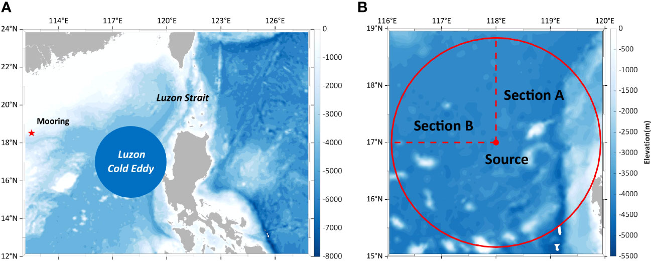
Figure 1 (A) Topography of the western Luzon Strait. The blue circular area represents the LCE and the pentagram represents the observation location. (B) Topography of the region near the LCE. The red solid circular region represents the horizontal calculation area of the acoustic model. The red dashed line represents the two sections in 90° and 180° direction. The red dots represent the horizontal position of sound source.

3.2 Model validation

Before conducting sound propagation modeling, the presence of the LCE and tide, including both barotropic and baroclinic tide, needs to be validated. For this purpose, the daily average temperature and salinity fields on January 23^rd from the model output are selected to diagnose the seawater sound speed. Specifically, 9 depth layers of 0 m, 50 m, 100 m, 150 m, 200 m, 300 m, 400 m, 600 m, 800 m are chosen to show the 3-D sound speed structure in the region between 14°-20°N, 115°-121°E (Figure 2). The structure of the LCE can be observed, exhibiting a horizontal scale of up to 400 km. The eddy core is roughly situated in 17°N, 118°E, where the sound speed reaches its minimum value in the region. In general, the eddy shape at a shallow depth of 200 m is relatively obvious. With the depth increasing, the eddy core gradually shifts, and the eddy structure becomes less distinct.

FIGURE 2

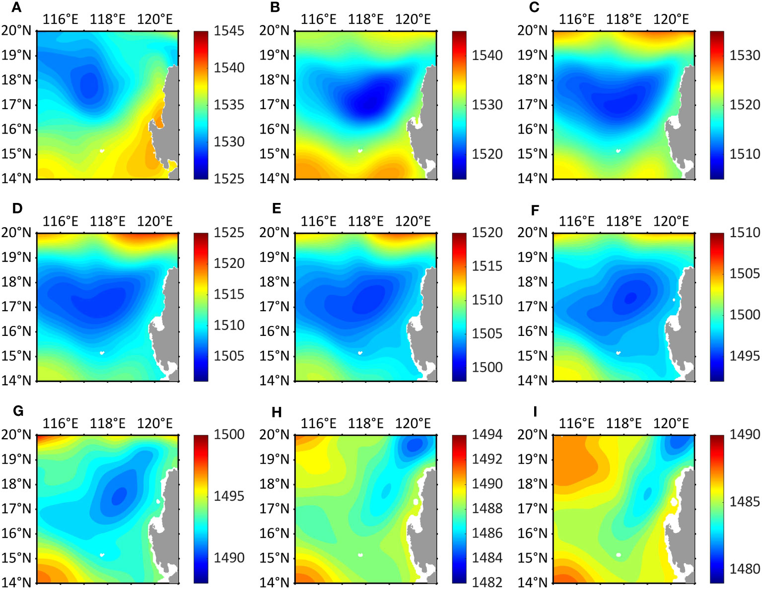
Figure 2 Sound speed around the cold eddy at (A) 0 m, (B) 50 m, (C) 100 m, (D) 150 m, (E) 200 m, (F) 300 m, (G) 400 m, (H) 600 m and (I) 800 m, respectively.

To further examine the sound speed characteristics near the eddy core, the sound speed anomaly is shown in Figure 3, indicating deviations from the case without the eddy, in two mutually perpendicular sections through the eddy core. As the depth is slightly shallower than 100 m, the eddy shape is more obvious near this depth (as seen in Figure 2). The largest sound speed anomaly reaches around 16 m/s at the core, and its corresponding latitude and longitude confirm the horizontal position of the eddy core.

FIGURE 3

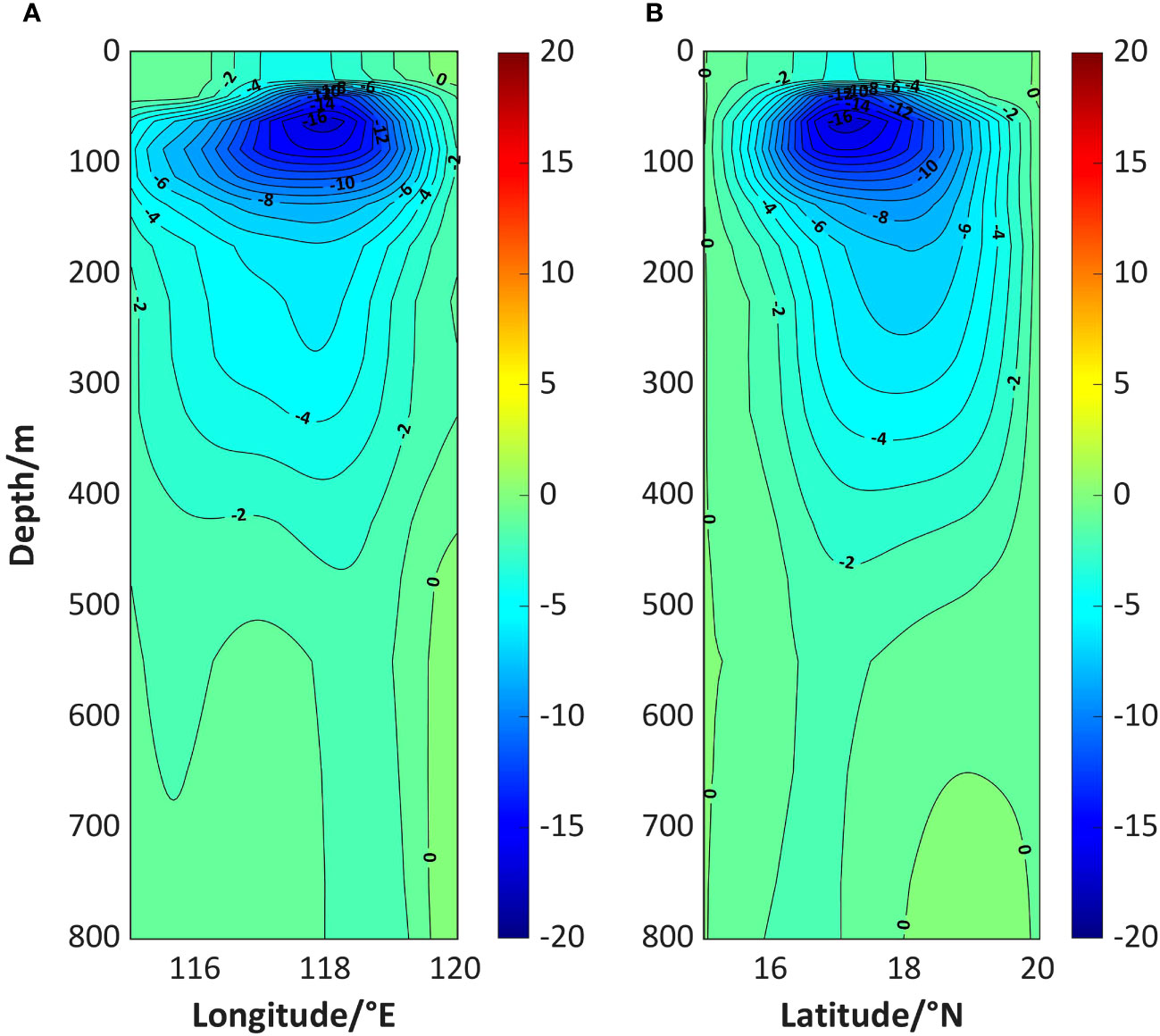
Figure 3 Sound speed profile anomaly on (A) meridional section and (B) zonal section across the core of the eddy (118°E, 17°N).

To validate the presence of tides, which are expected to be prevalent in the study region, a harmonic analysis is performed using the hourly SSH output from the model. The calculated amplitude and phase distributions of the K₁ and M₂ constituents are shown in Figures 4B, D, respectively, for the NSCS and the eastern Luzon Strait. By comparing the result with the harmonic constants from TPXO9 (Figures 4A, C), it can be observed that the simulation effectively captures while retaining the expected internal tide signal. This is evidenced by the small horizontal perturbations in amplitude and phase, confirming the accuracy of the tidal simulation.

FIGURE 4

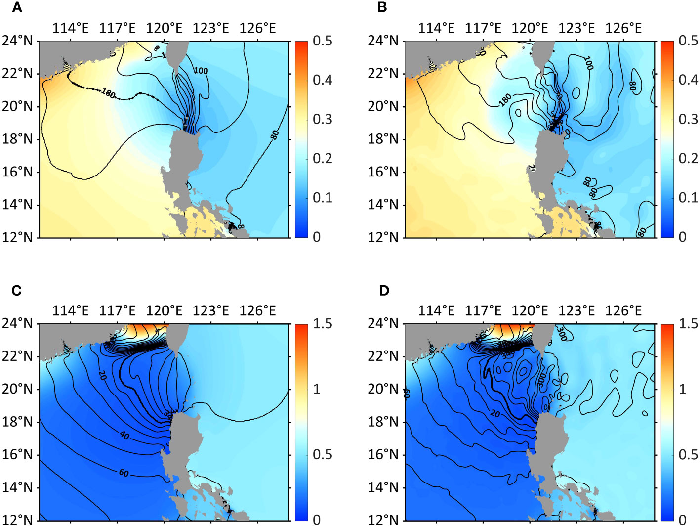
Figure 4 Comparison of harmonic constants between TPXO9 barotropic model and simulation result. (A) TPXO9 result for amplitude and phase of K₁ constituent. (B) Simulation result for amplitude and phase of K₁ constituent. (C) Same as (A), but of M₂ constituent. (D) Same as (B), but of M₂ constituent.

As mentioned in Section 1, it is possible to extract the internal tide signal from the variations in ocean hydrographic elements. To further confirm the presence of internal tide in the experimental region, the time series of the sound speed profiles at the eddy core (17°N, 118°E) within the upper 1000 m from January 20^th to 30^th is presented in Figure 5A. The fluctuations of the isosonic line induced by the internal tide can be clearly observed, which are most pronounced during spring tide, with amplitude reaching nearly 100 m. The periodicity of the fluctuations in the region is consistent with the features of the diurnal tide. In Figure 5B, the perturbation time series resulting from subtracting the 25-h running mean from the hourly sound speed profiles at the same location is shown. The small-scale periodic perturbations in the time series indicate the influence of the baroclinic tide.

FIGURE 5

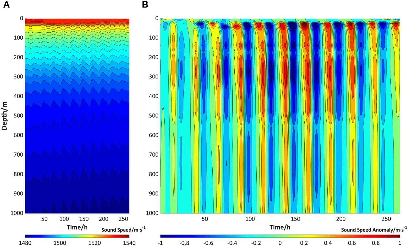
Figure 5 Time series of (A) sound speed profiles and (B) sound speed perturbation profiles in the upper 1000 m at the eddy core (118°E, 17°N) from the 20^th to the 30^th of January 2019.

A comparative analysis is conducted to further validate the accuracy of the simulated hydrographic field by comparing it with a series of observations from a moored buoy located in the NSCS (18˚31.180’N, 112˚30.037’E, represented by the pentagram in Figure 1A). During the entire simulation period of January 2019, temperature data from SBE recorded at a temporal resolution of 2 minutes and velocity data from ADCP recorded at a temporal resolution of 30 minutes have been quality controlled and are suitable for direct comparison.

Time-space matching between the simulation and observation is required by filtering the higher-frequency observations to obtain hourly data. The model result is then interpolated to the corresponding observation position and depths. The root-mean-square error (RMSE) is separately calculated for the temperature and current velocity profiles at each time and depth layer, focusing on the second half of the month when the model reaches a more stable state. The RMSE time series (Figure 6A, depth-averaged) and depth profiles (Figure 6B, time-averaged) demonstrate that the RMSE of temperature (red lines) and current velocity (blue and green lines) keeps always below 0.7°C and 0.2 m/s, respectively. These results generally confirm the accuracy of the model output. The model result actually reflects average state over cell grids and within time steps, therefore some high-frequency information may be lost compared to the instantaneous in-situ observations. Although it is reflected as the oscillations of the curves in Figure 6, the small temperature RMSE of less than 1°C indicates that the model result can provide reasonable data support for analyzing sound propagation characteristics within acceptable error limits.

FIGURE 6

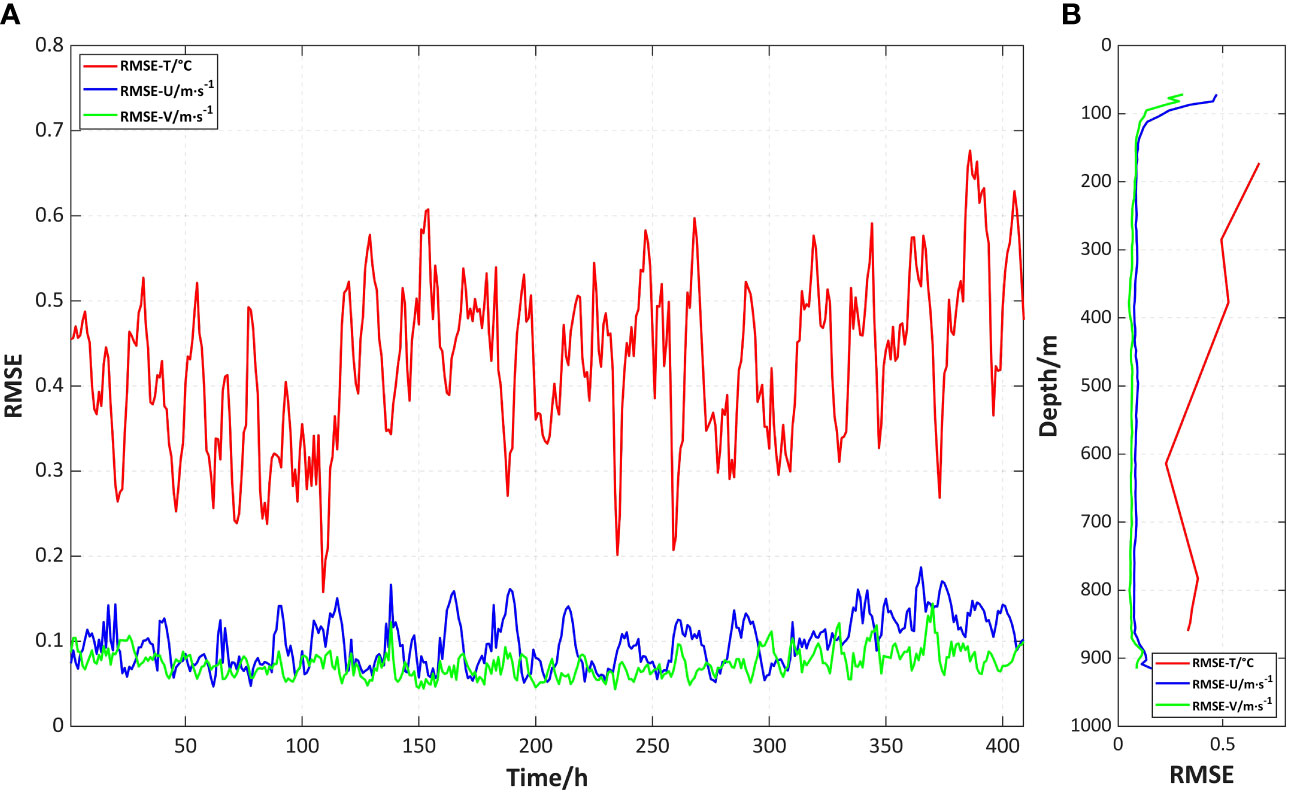
Figure 6 Validation result of simulation compared with observation. (A) RMSE time series of temperature and current velocity statistically by depth. (B) RMSE depth profile of temperature and current velocity statistically by time.

4 Sound propagation

The sound propagation in the coupled environment of the cold eddy and tide is investigated based on the BELLHOP model. The calculation region is shown as the red circle in Figure 1B, along with the corresponding distribution of water depth. The sound source is placed at the eddy core (17°N, 118°E), and the calculation radius covers approximately 200 km, encompassing the extent of the cold eddy. It is important to note that the topography on the eastern side of the region is more variable, which poses challenges for calculation of the sound field. Therefore, two representative sections oriented at 90° and 180° (with due east as 0°, following referred to as section A and section B, respectively) are primarily selected for sound propagation analysis. On this basis, the sound source is placed at 200 m for the convergence zone propagation pattern analysis and at 800 m for the deep-sea channel propagation pattern analysis, respectively (Zhang et al., 2020).

The sound speed diagnosed from seawater temperature, salt, pressure output from the ocean model in Section 3 is the crucial input for the model. In the environment configuration file, some certain parameters related to the sound field calculation are set as: water depth of 5250 m, sound source frequency of 1 kHz, density of 1.7 g/cm³, bottom sound speed of 1600 m/s, attenuation coefficient of 0.6 dB/λ (Li et al., 2019), elevation angle fan from -18° to 18°. The model output comprises sound pressure, ray and eigen ray traces, signal amplitude and arrival time structures, and allows for the calculation of transmission loss. To maximize the effect of tide on sound propagation, the experimental period is chosen to encompass the peak amplitude of the tidal waves during high tide. Specifically, January 23^rd to 24^th, which contains two tidal periods, is chosen as the experimental period, and four moments are taken every 12 h (8h, 20h, 32h, 44h) for sound propagation analysis. To comprehensively explore the effects of the coupled ocean environment, four separate sub-experiments are established, each with distinct characteristics as listed in Table 1, and more detailed analysis is presented below.

TABLE 1

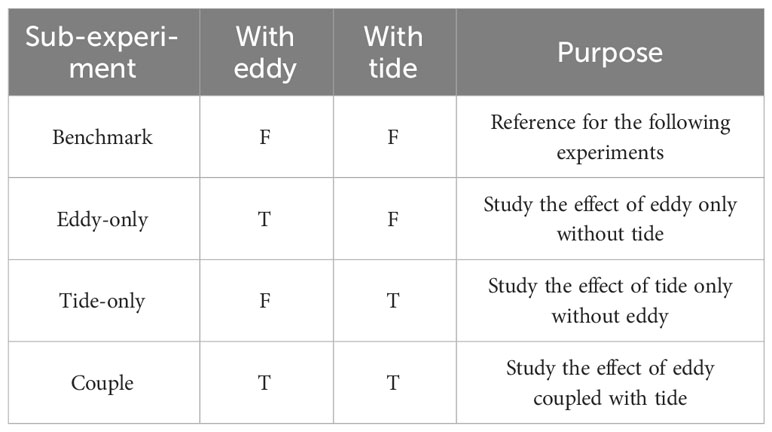
Table 1 Set-up of the four sound propagation experiments.

4.1 Sub-experiment a (benchmark)

The first sub-experiment serves as a benchmark for the comparative analysis of the remaining three cases. In this sub-experiment, the ocean model is driven without incorporating the tide generating potential forcing, while keeping other initial and boundary conditions unchanged to obtain the sound speed field with only the cold eddy signal (the sound speed field for sub-experiment b). After removing the eddy signal from the sound speed field in the experimental region, a spatial smoothing technique known as kriging interpolation is applied. Finally, the average sound speed field at four specific moments, which serves as the reference background field for the four sets of experiments, is imported into BELLHOP model.

Figure 7 shows the transmission loss in convergence zone propagation (Figures A–C) and deep-sea channel propagation (Figures 7D–F), respectively. It includes both the plane and section in the 90° and 180° directions (white dashed lines in Figures 7A, D), where the obvious convergence zone features can be observed. When the sound source is at 200 m, there are three convergence zones, whereas at a depth of 800 m, there are 4-5 convergence zones. The distribution of convergence zones in the benchmark sound field is not consistent in different directions. The reason for that may be the irregularity of the cold eddy, which exhibits a better shape in the shallow sea but shifts its position with depth. As a result, after smoothing out the eddy, a more obvious anisotropy is observed in the deep-sea environment. In this case, the rays propagate within the sound channel from 800 m to 1500 m, with stronger sound energy concentrated in the channel and lower transmission loss. In addition, the 2-D sound transmission loss pattern indicates that the sound rays are essentially spread throughout the region and can effectively interact with the cold eddy and ubiquitous internal tidal waves, which lays the fundamental basis for subsequent analysis.

FIGURE 7

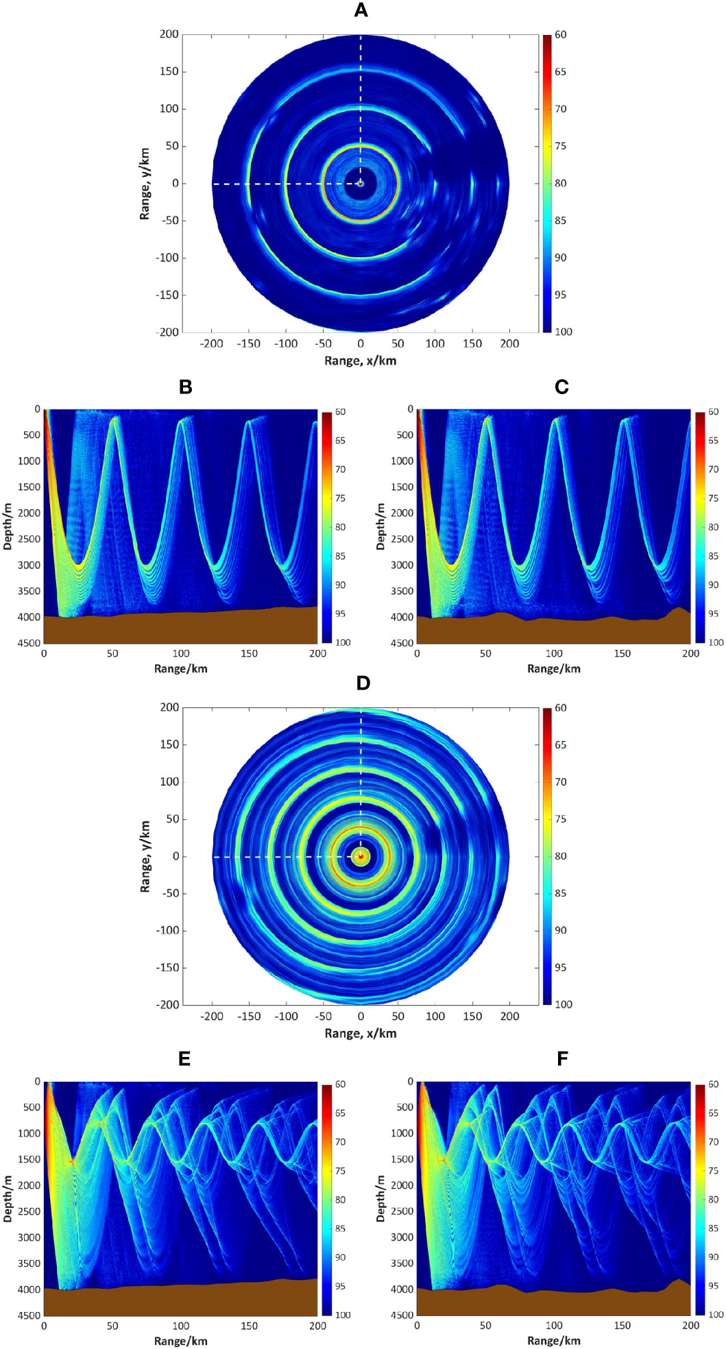
Figure 7 Sound transmission loss in the benchmark field. (A) 2-D transmission loss at 200 m when SD = 200 m. (B) 2-D transmission loss on section A when SD = 200 m. (C) Same as (B), but on section (B). (D) Same as (A), but SD = 800 m. (E) Same as (B), but SD = 800 m. (F) Same as (C), but SD = 800 m.

4.2 Sub-experiment b (eddy-only)

In this sub-experiment, the study is conducted using the sound speed field affected by the presence of the LCE only, as described in the previous sub-experiment. The distribution of sound speed anomaly on the two sections corresponds to Figure 3, which contains the extensions of Section A and B. For a greater intuition of the analysis, the 1-D transmission loss curves at the source depth for each case are presented (Figure 8), which are low-pass filtered to eliminate the effect of some high-frequency disturbances. When the source and receiver depth are both 200 m (Figures 8A, B, convergence zone propagation), the convergence zone in the calculated region exhibits a maximum forward shift of 5 km. This shift is attributed to the lower temperature around the core of the cold eddy, which increases the refraction of rays towards this region. The conclusion is consistent with the results of previous studies (Jian et al., 2009; Li et al., 2011; Ruan et al., 2019; Xiao et al., 2019; Chen et al., 2019; Zhang et al., 2020). However, when the source depth is 800 m (Figures 8C, D, deep-sea channel propagation), the shift decreases to 3 km in section A, while almost reaches 15 km on section B, which can be explained in two ways. On the one hand, the cold eddy is of smaller intensity and the position of the eddy core has shifted at 800 m, leading to a smaller forward shift compared to that in the convergence zone propagation pattern at 200 m. On the other hand, the black curve representing the benchmark on section B (Figure 8D) demonstrates a greater backward shift compared to that on section A (Figure 8C), which aligns with the explanation in sub-experiment a, resulting in the abnormally large forward shift on section B.

FIGURE 8

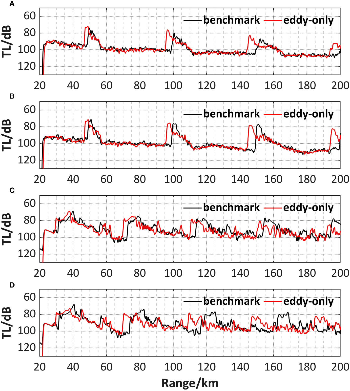
Figure 8 Comparison of 1-D transmission loss of sound propagation from the core of the cold eddy and in the benchmark field when when (A) SD = RD = 200 m on section A, (B) SD = RD = 200 m on section B, (C) SD = RD = 800 m on section A, (D) SD = RD = 800 m on section B (RD receiver depth).

Next, an analysis of the multipath arrival structure is conducted (Figure 9), focusing on the two cases with a source depth of 200 m and 800 m, respectively. Firstly, the effect on the amplitude is discussed (Figures 9A–D). At the depth of 200 m, the ray is significantly affected by the cold eddy, resulting in certain groups of arrival structures being enhanced while the amplitude of the remaining arrival structures is smaller. However, this difference is less obvious at the depth of 800 m. Consequently, the cold eddy has a discernible impact on the energy distribution of each group of arrival structures in sound propagation, leading to a more concentrated energy distribution on a few arrival structures.

FIGURE 9

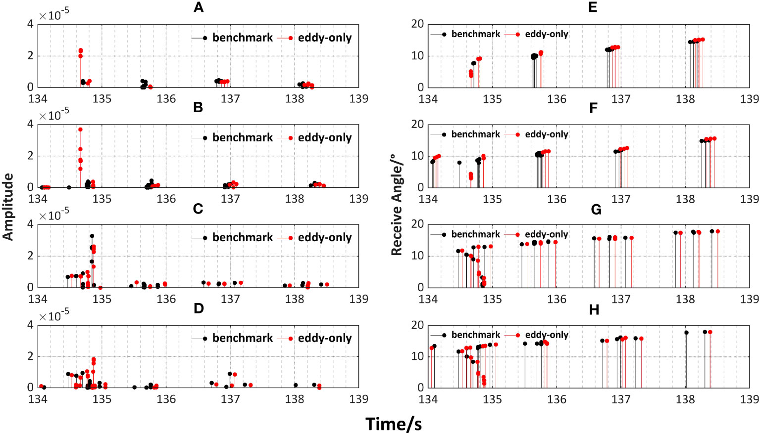
Figure 9 Comparison of arrival structures of sound propagation from the core of the cold eddy and in the benchmark field, including arrival amplitude when (A) SD = RD = 200 m on section A, (B) SD = RD = 200 m on section B, (C) SD = RD = 800 m on section A, (D) SD = RD = 800 m on section B and receive angle when (E) SD = RD = 200 m on section A, (F) SD = RD = 200 m on section B, (G) SD = RD = 800 m on section A,(H) SD = RD = 800 m on section B..

An analysis combined with the arrival angle (Figures 9E–H) reveals that in the presence of the cold eddy, the amplitude and reception angle of the first few groups of arrivals differ significantly from the benchmark field, while the other arrivals tend to overlap each other. As the arrival time increases, the grazing angle gradually increases from less than 15° to nearly 20°. This suggests that the smaller grazing angle of the first few arrivals compared to the later groups may be the reason for their greater susceptibility to the influence of the cold eddy. In addition, it is obvious that the arrivals are delayed compared to the corresponding benchmark arrivals due to the cold eddy, although the magnitude of the delay is not significant, reaching about 0.1 s.

4.3 Sub-experiment c (tide-only)

The sound speed field of this sub-experiment is obtained by adding the tide signal, derived from the difference between the sound speed field with and without the tidal generation potential forcing, to the benchmark sound speed field in sub-experiment a. Therefore, it is considered to contain only the disturbance of the tide without the cold eddy. As mentioned earlier, the motion of the tidal waves in the sound propagation process is ignored and it is assumed to be “frozen” in time due to the long period of the astronomical tide. Four specific moments are selected as the background sound speed field, which is imported into BELLHOP for sound propagation analysis. The 1-D transmission loss curves at two source depths are also presented for comparison (Figure 10).

FIGURE 10

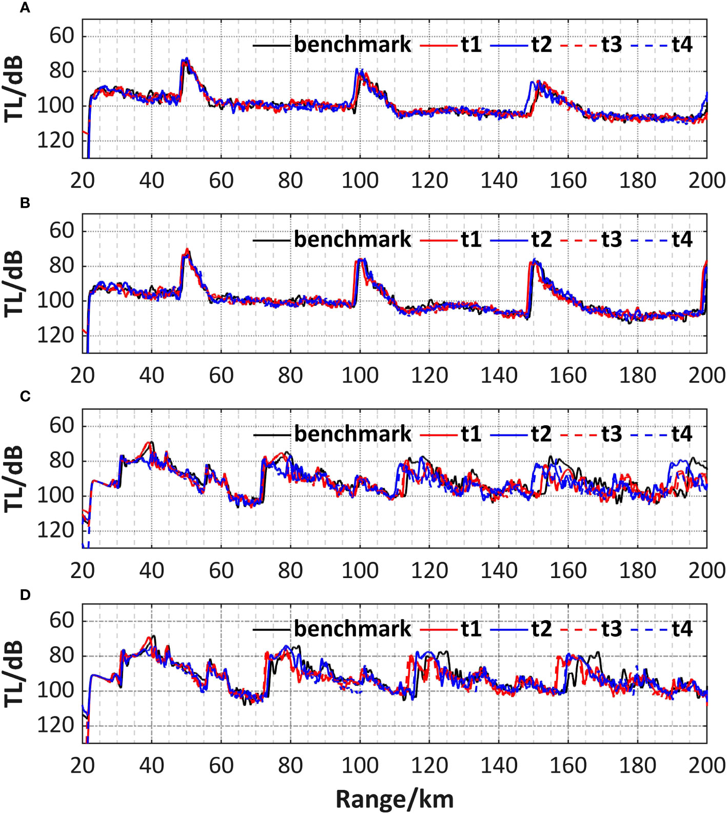
Figure 10 Comparison of 1-D transmission loss of sound propagation in the background field with tide at four moments and in the benchmark field when(A) SD = RD = 200 m on section A, (B) SD = RD = 200 m on section B, (C) SD = RD = 800 m on section A, (D) SD = RD = 800 m on section B.

Under the influence of the tide, the transmission loss curves fluctuate periodically. The red curves (representing t1 and t3) and the blue curves (representing t2 and t4) correspond well to each other, reflecting the tidal periodic characteristics in the sea. To further explore the reason for the variation in transmission loss, the sound speed difference between the field with tide and the benchmark field in sub-experiment a is made, resulting in the sound speed anomaly at four moments on sections A and B (Figure 11). The anomaly corresponds to the periodic variations in the transmission loss. Moreover, regardless of the input background sound speed field at any given time, the convergence zone shifts forward to some extent, primarily due to the rise of the isosonic plane, indicating that the sound speed anomaly is generally negative throughout a tidal period. It could be attributed to the cold advection caused by tidal current, indirectly leading to a reduction of sound speed in the region. This effect incorporates the contribution of both barotropic tide and internal tide. The overall impact is similar to that caused by the cold eddy, leading to a similar result as observed in sub-experiment b, although the intensity is not as pronounced. When the source is at 200 m, the maximum forward distance in the calculated region is about 2.5 km. However, when the source is at 800 m, the forward distance can reach about 5 km, which is probably due to the larger amplitude of the internal tidal waves at greater depth compared to shallow seas (Figure 5A).

FIGURE 11

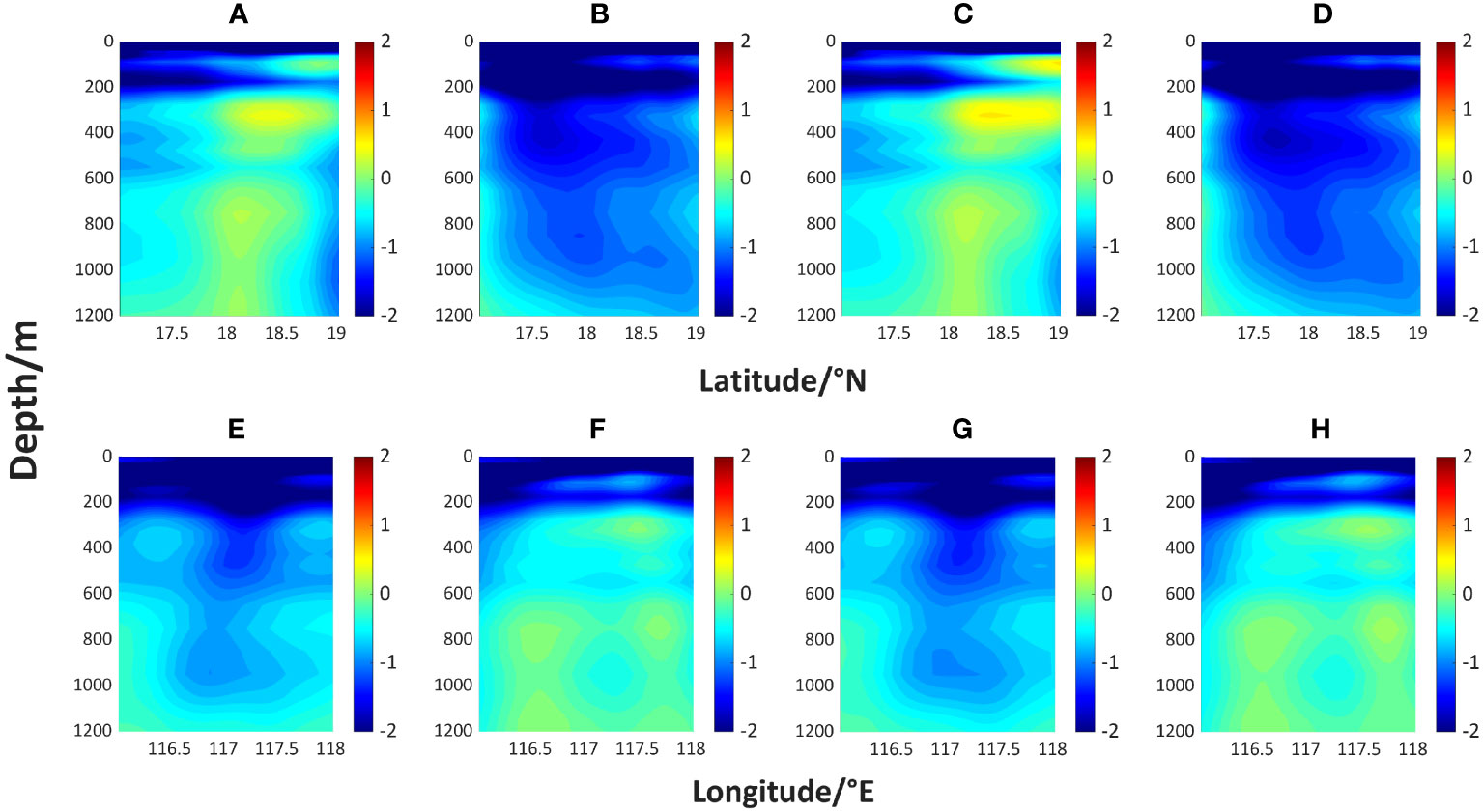
Figure 11 Sound speed anomaly in section A at (A) t1, (B) t2, (C) t3, (D) t4, and section B at (E) t1, (F) t2, (G) t3, (H) t4, respectively.

It is worth noting that regardless of whether the source is at 200 m or 800 m, the red curves for t1 and t3 appear ahead, while the blue curves for t2 and t4 lag behind at section A. However, at section B, the order of these two types of curves is reversed. It seems to indicate the opposite characteristics of the sound propagation fluctuations caused by the tidal waves at the same moment on the two sections, which can be explained by the distribution of the sound speed anomaly on the sections. Figure 11 indicates the sound speed anomaly is predominantly positive at t1 and t3 on section A, while they are mostly negative at t2 and t4. Conversely, the pattern on section B is opposite. It can be attributed to the spatial propagation of the tidal waves. As for t1 and t3, section A may experience low tide while section B encounters high tide. The situation is reversed at t2 and t4, resulting in an interesting “rising and falling” pattern. This results in an increase in the convergence zone forward distance of about 2-3 km at high tide compared to that at low tide.

The same analysis of the multipath arrival structures is performed. Figures 12A, B, E, F correspond to the signal amplitude and arrival angle at 200 m, respectively. Figures 12C, D, G, H correspond to the signal amplitude and arrival angle at 800 m, respectively. Due to the periodicity of the tide, the arrivals that are one tidal period apart exhibit better alignment. Additionally, it is evident that, similar to the cold eddy environment, the tide also affects the energy distribution of the arrivals within each group during sound propagation. It is reflected by a greater concentration of energy on a few specific arrivals, especially in the convergence zone propagation pattern where the arrival angles are smaller. It can also be inferred that the smaller grazing angle contributes to the stronger influence of the tide on the first few groups of arrivals. Regarding the influence of the tidal waves on the delay of acoustic signal arrivals, regardless of the input background sound speed field at any given time, the arrivals experience only a limited delay, and the magnitude of the delay remains small. It is not as obvious as in sub-experiment b. The order of the red lines representing t1 and t3 and the blue lines representing t2 and t4 on the two sections remains opposite, which corresponds to the pattern observed in the transmission loss curves and further reflects the spatial propagation characteristic of the tidal waves. This characteristic leads to the periodic fluctuation of the acoustic signal.

FIGURE 12

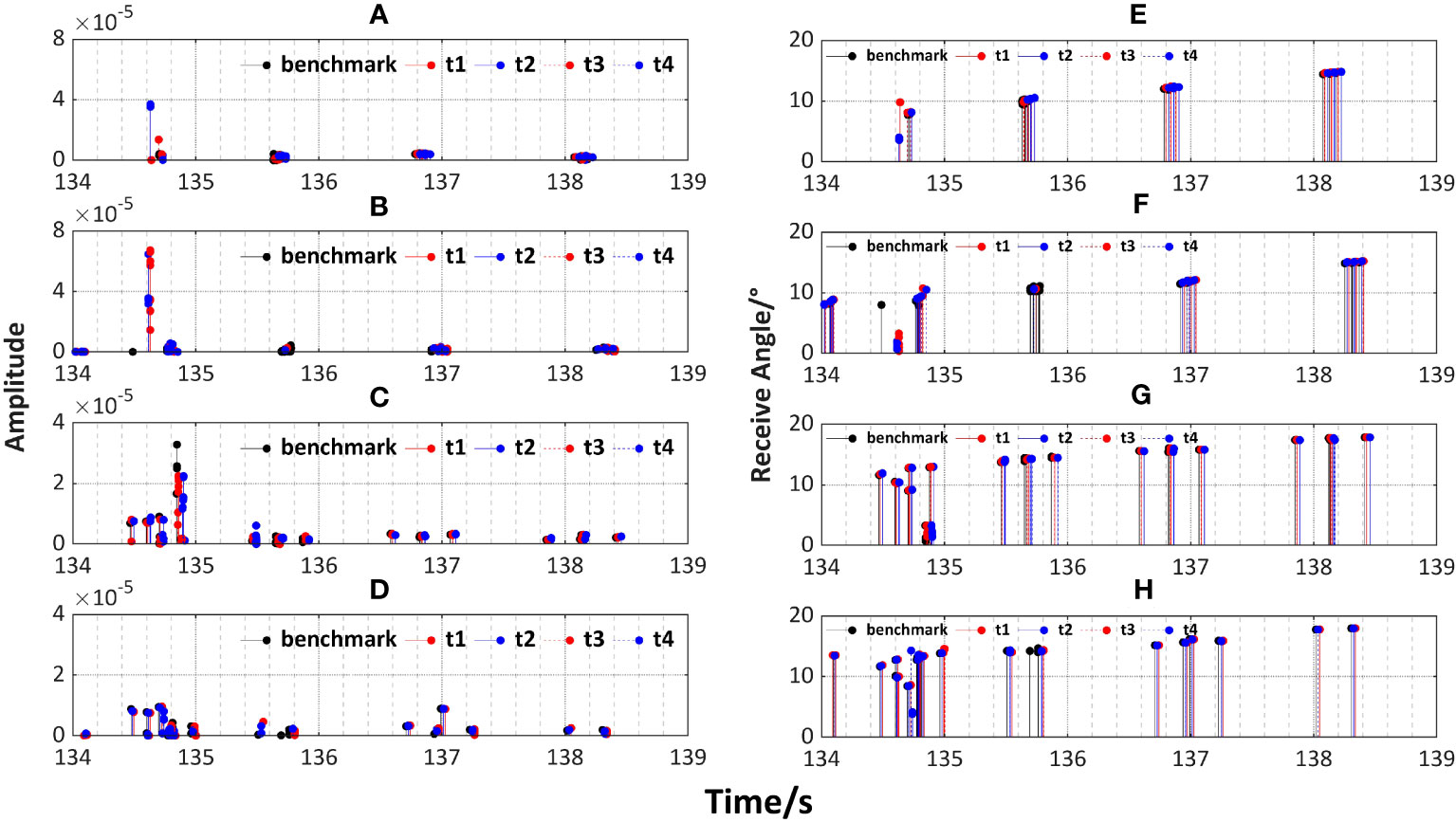
Figure 12 Comparison of arrival structures of sound propagation in the background field with tide at four moments and in the benchmark field, including arrival amplitude when (A)SD = RD = 200 m on section A,(B)SD = RD = 200 m on section B, (C)SD = RD = 800 m on section A, (D) SD = RD = 800 m on section B and receive angle when (E) SD = RD = 200 m on section A, (F) SD = RD = 200 m on section B,(G) SD = RD = 800 m on section A, (H) SD = RD = 800 m on section B.

4.4 Sub-experiment d (couple)

The sound speed field used in this sub-experiment is the baroclinic field obtained directly from numerical simulation, representing the complex ocean environment resulting from the interaction of the LCE and tide. Similar to sub-experiment c, the motion of the tidal waves during sound propagation is neglected, and the sound speed field at the same four moments is selected for the sound propagation analysis. For comparative analysis, the transmission loss curves at the source depth are given as well (Figure 13).

FIGURE 13

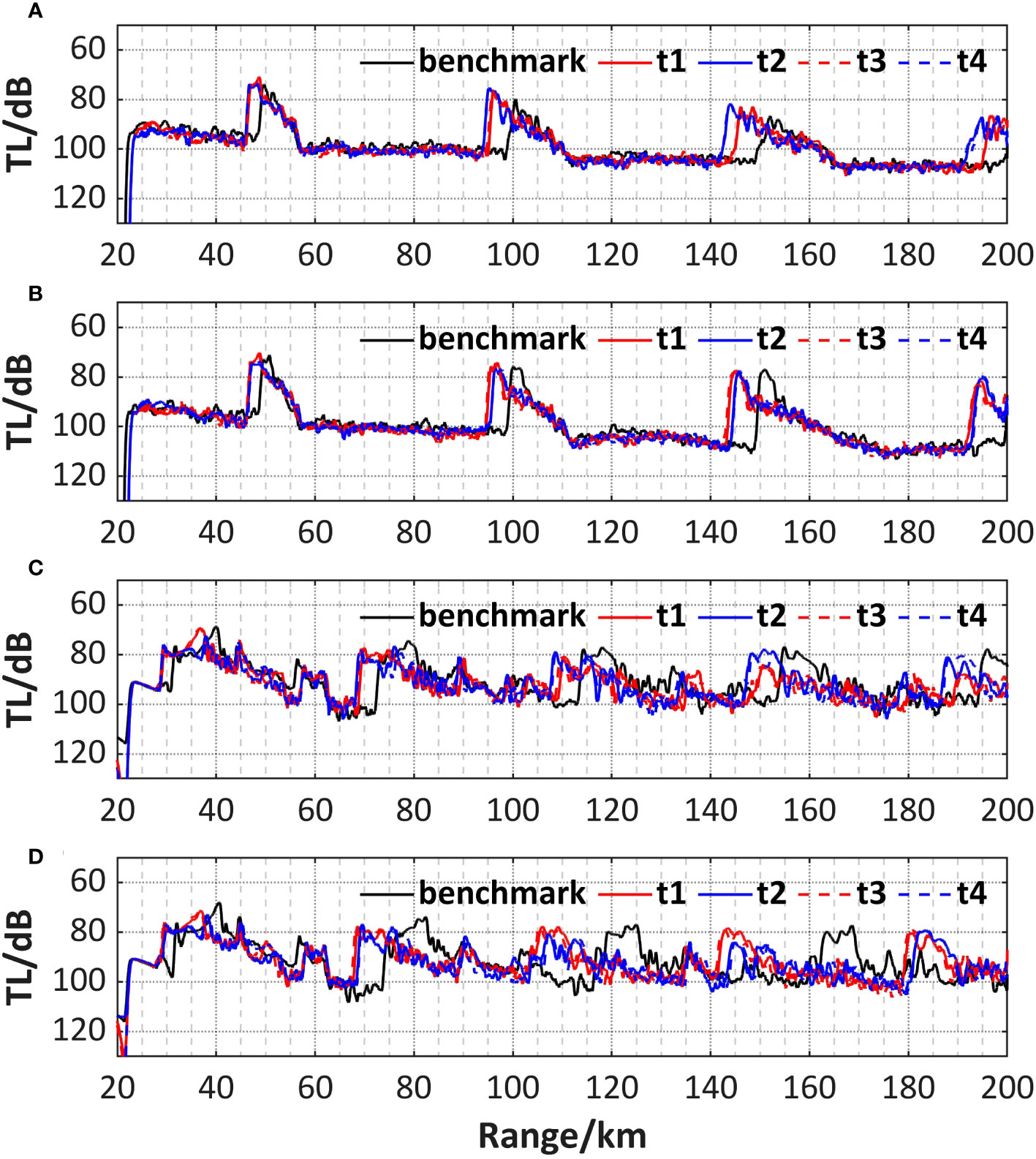
Figure 13 Comparison of 1-D transmission loss of sound propagation in the coupled background field at four moments and in the benchmark field when (A) SD = RD = 200 m on section A,(B) SD = RD = 200 m on section B, (C) SD = RD = 800 m on section A, (D) SD = RD = 800 m on section B.

In general, the convergence zone of the sound field at each moment still shifts forward compared to the benchmark background field. Compared to when only the cold eddy is present, the maximum distance of the convergence zone at the two source depths increases by about 2.5 and 5 km, respectively, which is attributed to the perturbation of sound speed field by the tide. Furthermore, the solid and dashed curves of the same color still exhibit good agreement, and the phenomenon of the red and blue curves having opposite order on the two sections reappears. This observation aligns with the pattern observed in sub-experiment c, which is closely related to the spatial propagation characteristics of the tidal waves.

Next, the multipath arrival structures in the coupled environment are analyzed. The amplitude and arrival angle of the acoustic signal at two source depths and two sections are present in Figures 14A-D and Figures 14E-H, respectively. The acoustic energy continues to be converged in the first few groups of arriving structures, which is consistent with the findings from sub-experiments b and c, indicating the combined effect by cold eddy and tide. Except for the first few groups, the received angles of the later groups are extremely similar, from which the propagation delay of the acoustic signal can also be observed. Since both the cold eddy and tide contribute to the delay of the acoustic signal arrival, with the coupling of these two dynamic processes, the delay becomes more noticeable, especially high tide moments (t2 and t4 for section A, t1 and t3 for section B). In general, the impact of the cold eddy on the arrival structures is more significant compared to that of tide, where the tide serves as a periodic, small-amplitude perturbation of the sound field.

FIGURE 14

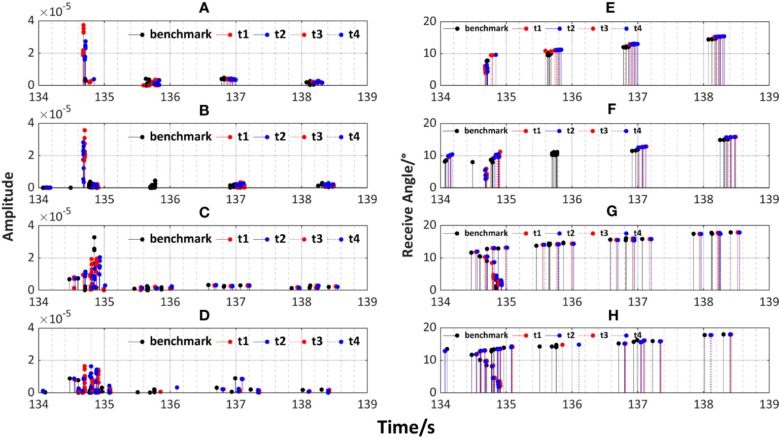
Figure 14 Comparison of arrival structures of sound propagation in the coupled background field at four moments and in the benchmark field, including arrival amplitude when (A) SD = RD = 200 m on section A, (B) SD = RD = 200 m on section B, (C) SD = RD = 800 m on section A, (D)SD = RD = 800 m on section B and receive angle when (E)SD = RD = 200 m on section A, (F)SD = RD = 200 m on section B, (G) SD = RD = 800 m on section A, (H) SD = RD = 800 m on section B.

5 Conclusion

The purpose of the research is to investigate the sound propagation characteristics in a region under the coupled influence of eddy and tide, which has received limited attention in previous research. Initially, the LCE and tide field near the study region during January 2019 are reconstructed based on MITgcm. Subsequently, based on the hydrographic field from the 3-D baroclinic tide model, the sound speed field is calculated using an empirical formula. After applying spatial smoothing and other necessary operations, the benchmark, eddy-only, tide-only, and coupled sound speed fields are obtained, which are then imported into the BELLHOP model for deep-sea sound propagation simulation.

Two cases are examined in this study, with the sound source at 200 m and 800 m, respectively. The focus is on two sections crossing the core of the cold eddy. The results indicate that both cold eddy and tide can influence the sound speed profile, causing the convergence zone to shift forward and closer to the source. In the complicated ocean environment where both phenomena exist, the effect on the convergence zone is more significant. Since the fluctuation of the tidal waves on the sound speed profile is periodic, the contribution to the forward shift of the convergence zone of the sound field varies at different times during the tidal period. The maximum forward shift occurs when the sound speed profile is most significantly elevated during high tide, resulting in the strongest ability to focus acoustic energy. At its peak, the convergence zone further shifted forward by about 2-3 km compared to low tide. Additionally, considering that tidal waves propagate at a specific spatial scale in the ocean, the fluctuation by tide varies at different locations even at the same time. This is reflected in the experiments as the opposite effects of high and low tide in the two sections.

The modeling results of the multipath arrival structure demonstrate that the rays of the first few arrivals usually propagate at smaller grazing angles, resulting in more frequent interactions with eddy and tidal waves. As a result, the rays of the first few arrivals were often more significantly affected compared to those of the later arrivals. This indicates that the energy tends to be more concentrated in the first few arrivals of the sound field. Furthermore, both the cold eddy and tide contribute to the delay of most arrivals. In the environment simulated in this study, the coupled influence of these two dynamic processes can cause a maximum delay of approximately 0.12 s in the arrivals. Considering the periodicity and spatial correlation of the tidal waves, the delay at the same position varies slightly at different times, corresponding to the rise and fall of the tide. The delay is more significant during high tide compared to low tide. At the same moment, the amplitude of the tidal waves varies at different positions, resulting in variations in the time delay. This pattern is in agreement with the spatial and temporal variation observed in the 1-D transmission loss curve. In summary, the effect of tide on sound propagation could be considered as a new spatial and temporal disturbance superimposed on the stable disturbance caused by the LCE.

The results in this study primarily show the effect of the LCE and tide on sound propagation in the real ocean. Future work should focus on examining the long-term evolution of the LCE. Additionally, it is important to explore the contributions of other small or mesoscale processes in ocean sound propagation. This study serves as a reference for sound propagation modeling considering ocean dynamic mechanisms. Furthermore, a potential development in the future is the creation of an online coupled ocean-acoustic model. Such a model would be tailored for underwater detection and localization purposes, providing quasi-real-time or forecasted acoustic field information in a real ocean environment.

Data availability statement

The datasets presented in this article are not readily available because The dataset is too large and not available for commercial usage. Requests to access the datasets should be directed to Yu Liu, rjly1005@163.com.

Author contributions

YL: Writing – original draft. XZ: Writing – review & editing. HF: Writing – review & editing. ZQ: Writing – review & editing.

Funding

The author(s) declare financial support was received for the research, authorship, and/or publication of this article. The research is supported by grants from the National Key Research and Development Program of China (No. 2021YFC2803003).

Acknowledgments

We are grateful for the observations shared by the National Basic Research Program of China (No. 2013CB430304).

Conflict of interest

The authors declare that the research was conducted in the absence of any commercial or financial relationships that could be construed as a potential conflict of interest.

Publisher’s note

All claims expressed in this article are solely those of the authors and do not necessarily represent those of their affiliated organizations, or those of the publisher, the editors and the reviewers. Any product that may be evaluated in this article, or claim that may be made by its manufacturer, is not guaranteed or endorsed by the publisher.

Supplementary material

The Supplementary Material for this article can be found online at: https://www.frontiersin.org/articles/10.3389/fmars.2023.1278333/full#supplementary-material

References

Alford M. H., Mackinnon J. A., Nash J. D., Simmons H., Pickering A., Klymak J. M., et al. (2011). Energy flux and dissipation in Luzon Strait: Two tales of two ridges. J. Phys. Oceanogr. 41 (11), 2211–2222. doi: 10.1175/JPO-D-11-073.1

CrossRef Full Text | Google Scholar

Baer R. N. (1980). Calculations of sound propagation through an eddy. J. Acoustical Soc. America 67 (4), 1180–1185. doi: 10.1121/1.384178

CrossRef Full Text | Google Scholar

Baer R. N. (1981). Propagation through a three-dimensional eddy including effects on an array. J. Acoustical Soc. America 69 (1), 70–75. doi: 10.1121/1.385253

CrossRef Full Text | Google Scholar

Cao Z., Zhang Y., Li Q., Liu P. (2018). Impact of seasonal factors on the acoustic propagation in Atlantic Ocean. J. Appl. Oceanogr. (in Chinese). 37(4), 514–524. doi: 10.3969/j.issn.2095-4972.2018.04.007

CrossRef Full Text | Google Scholar

Chang Y., Huang C., Chen C., Sen J. (2012). Study of transmission loss variation affected by internal tides in the sea area northeast of Taiwan. J. Comput. Acoust. 20 (01), 1250002. doi: 10.1142/S0218396X1100450X

CrossRef Full Text | Google Scholar

Chen C., Gao Y., Yan F., Jin T., Zhou Z. (2019). Delving into the two-dimensional structure of a cold Eddy east of Taiwan and its impact on acoustic propagation. Acoust. Aust. 47 (2), 185–193. doi: 10.1007/s40857-019-00160-7

CrossRef Full Text | Google Scholar

Chen C.-T., Millero F. J. (1977). Speed of sound in seawater at high pressures. J. Acoustical Soc. America 62 (5), 1129–1135. doi: 10.1121/1.381646

CrossRef Full Text | Google Scholar

Chen M., Chen X., Zhang H., Gong Y., Zhang Z. (2018). Modelling of Internal Tides Originating and Propagating in the South China Sea. J. Ocean Univ. China.

Google Scholar

Chu X., Chen G., Qi Y. (2020). Periodic mesoscale eddies in the South China Sea. J. Geophys. Res.: Oceans 125 (1), e2019JC015139. doi: 10.1029/2019JC015139

CrossRef Full Text | Google Scholar

D’Asaro E. A., Lien R.-C., Henyey F. (2007). High-frequency internal waves on the Oregon continental shelf. J. Phys. Oceanogr. 37 (7), 1956–1967. doi: 10.1175/JPO3096.1

CrossRef Full Text | Google Scholar

Duda T. F., Lynch J. F., Irish J. D., Beardsley R. C., Ramp S. R., Chiu C. S., et al. (2004). Internal tide and nonlinear internal wave behavior at the continental slope in the northern south China Sea. IEEE J. Oceanic Eng. 29 (4), 1105–1130. doi: 10.1109/JOE.2004.836998

CrossRef Full Text | Google Scholar

Fang Y., Hou Y., Jing Z. (2015). Seasonal characteristics of internal tides and their responses to background currents in the Luzon Strait. Acta Oceanologica Sin. 34 (11), 46–54. doi: 10.1007/s13131-015-0747-z

CrossRef Full Text | Google Scholar

Fu H., Wu X., Li W., Zhang L., Liu K., Dan B. (2021). Improving the accuracy of barotropic and internal tides embedded in a high-resolution global ocean circulation model of MITgcm. Ocean Model. 162 (C12), 101809. doi: 10.1016/j.ocemod.2021.101809

CrossRef Full Text | Google Scholar

Gul S., Zaidi S.S. H., Khan R., Wala A. B. (2017). “Underwater acoustic channel modeling using BELLHOP ray tracing method,” in 2017 14th International Bhurban Conference on Applied Sciences and Technology (IBCAST). (Islamabad, Pakistan: IEEE). doi: 10.1109/IBCAST.2017.7868122

CrossRef Full Text | Google Scholar

Guo P., Fang W., Yu H. (2006). Progress in the observational studies of internal tide over continental shelf. Adv. Earth Sci. (in Chinese) 21 (6), 617–624. doi: 10.3321/j.issn:1001-8166.2006.06.009

CrossRef Full Text | Google Scholar

Guo S., Hu T. (2010). Simulating the effects of the internal tide in the Yellow Sea on acoustic propagation. J. Harbin Eng. Univ. (in Chinese) 31 (7), 967–974. doi: 10.3969/j.issn.1006-7043.2010.07.025

CrossRef Full Text | Google Scholar

Hassantabar B. S. H., Ciani D., Mahdizadeh M. M., Akbarinasab M., Aguiar A. C.B., Peliz A., et al. (2021). Effect of subsurface mediterranean water eddies on sound propagation using ROMS output and the bellhop model. Water 13 (24), 3617. doi: 10.3390/w13243617

CrossRef Full Text | Google Scholar

Hosseini S. H., Akbarinasab M., Khalilabadi M. R. (2018). Numerical simulation of the effect internal tide on the propagation sound in the Oman Sea. J. Earth Space Phys. 44 (1), 215–225. doi: 10.22059/jesphys.2018.221834.1006867

CrossRef Full Text | Google Scholar

Jan S., Lien R.-C., Ting C.-H. (2008). Numerical study of baroclinic tides in Luzon Strait. J. Oceanogr. 64 (5), 789–802. doi: 10.1007/s10872-008-0066-5

CrossRef Full Text | Google Scholar

Jian Y., Zhang J., Liu Q. S., Wang Y. F. (2009). Effect of mesoscale eddies on underwater sound propagation. Appl. Acoust. 70 (3), 432–440. doi: 10.1016/j.apacoust.2008.05.007

CrossRef Full Text | Google Scholar

Jiang R., Cao S., Xue C., Lixing T. (2017). “Modeling and analyzing of underwater acoustic channels with curvilinear boundaries in shallow ocean,” in 2017 IEEE International Conference on Signal Processing, Communications and Computing (ICSPCC). (Xiamen, China: IEEE). doi: 10.1109/ICSPCC.2017.8242476

CrossRef Full Text | Google Scholar

Jiang L., Hu J. (2010). Seasonal variability of the Luzon cold eddy and its relation with wind stress. J. Oceanogr. Taiwan Strait (in Chinese) 29 (1), 114–121. doi: 10.3969/J.ISSN.1000-8160.2010.01.017

CrossRef Full Text | Google Scholar

Li B., Cao A., Lv X. (2015). Three-dimensional numerical simulation of M2 internal tides in the Luzon Strait. Acta Oceanologica Sin. 34 (11), 55–62. doi: 10.1007/s13131-015-0748-y

CrossRef Full Text | Google Scholar

Li M., Hou Y., Li Y., Hu P. (2012). Energetics and temporal variability of internal tides in Luzon Strait: a nonhydrostatic numerical simulation. Chin. J. Oceanol. Limnol. 30 (5), 852–867. doi: 10.1007/s00343-012-1289-2

CrossRef Full Text | Google Scholar

Li M., Li Z., Li Q. (2019). Geoacoustic inversion for bottom parameters in a thermocline environment in the northern area of the South China Sea. Chin. J. Acoust. (in Chinese) 39 (1), 14. doi: 10.15949/j.cnki.0371-0025.2019.03.006

CrossRef Full Text | Google Scholar

Li S., Li Z., Li W., Qin J. (2018). Horizontal refraction effects of seamounts on sound propagation in deep water. Haiyang Xuebao (in Chinese) 67 (22), 216–226. doi: 10.7498/aps.67.20181480

CrossRef Full Text | Google Scholar

Li J., Zhang R., Chen Y., Jin B. (2011). Ocean mesoscale eddy modeling and its application in studying the effect on underwater acoustic propagation. Mar. Sci. Bull. (in Chinese). 30 (1), 37–46. doi: 10.3969/j.issn.1001-6392.2011.01.007

CrossRef Full Text | Google Scholar

Lin P., Wang F., Chen Y., Tang X. (2007). Temporal and spatial variation characteristics on eddies in the South China Sea I. Statistical analyses. Haiyang Xuebao (in Chinese) 29 (3), 14–22. doi: 10.3321/j.issn:0253-4193.2007.03.002

CrossRef Full Text | Google Scholar

Liu J., Mao K., Yan M., Zhang X., Shi Y. (2006). The general distribution characteristics of thermocline of China Sea. Mar. Forecasts (in Chinese). 23 (2), 39–44. doi: 10.3969/j.issn.1003-0239.2006.02.005

CrossRef Full Text | Google Scholar

Liu K., Xu Z., Yin B. (2017). Three-dimensional numerical simulation of internal tides that radiated from the Luzon Strait into the Western Pacific. Chin. J. Oceanol. Limnol. 35 (6), 1275–1286. doi: 10.1007/s00343-017-5376-2

CrossRef Full Text | Google Scholar

Mahpeykar O., Larki A. A., Nasab M. A. (2022). The effect of cold eddy on acoustic propagation (Case study: Eddy in the Persian Gulf). Arch. Acoust. 47 (3), 413–423. doi: 10.24425/aoa.2022.142015

CrossRef Full Text | Google Scholar

Marshall J., Adcroft A., Hill C., Perelman L., Heisey C. (1997). A finite-volume, incompressible Navier Stokes model for studies of the ocean on parallel computers. J. Geophys. Res.: Oceans 102 (C3), 5753–5766. doi: 10.1029/96JC02775

CrossRef Full Text | Google Scholar

Niwa Y., Hibiya T. (2004). Three-dimensional numerical simulation of M2 internal tides in the East China Sea. J. Geophys. Res.: Oceans 109 (C4). doi: 10.1029/2003JC001923

CrossRef Full Text | Google Scholar

Noufal K. K., Sanjana M. C., Latha G., Ramesh R. (2022). Influence of internal wave induced sound speed variability on acoustic propagation in shallow waters of North West Bay of Bengal. Appl. Acoust. 194, 108778. doi: 10.1016/j.apacoust.2022.108778

CrossRef Full Text | Google Scholar

Oba R., Finette S. (2002). Acoustic propagation through anisotropic internal wave fields: Transmission loss, cross-range coherence, and horizontal refraction. J. Acoustical Soc. America 111 (2), 769–784. doi: 10.1121/1.1434943

CrossRef Full Text | Google Scholar

Porter M. B., Bucker H. P. (1987). Gaussian beam tracing for computing ocean acoustic fields. J. Acoustical Soc. America 82 (4), 1349–1359. doi: 10.1121/1.395269

CrossRef Full Text | Google Scholar

Qu T. (2002). Evidence for water exchange between the South China Sea and the Pacific Ocean through the Luzon Strait. Acta Oceanologica Sin. 2), 175–185.

Google Scholar

Ruan H., Yang Y., Wen H., Xie X., Niu F. (2019). “Analysis the influence of a mesoscale cold eddy on underwater sound propagation in the east of Luzon Strait,” in 2nd International Conference on Information, Communication and Engineering (in Chinese). doi: 10.35745/icice2018v2.031

CrossRef Full Text | Google Scholar

Saunders P. M. (1981). Practical conversion of pressure to depth. J. Phys. Oceanogr. 11 (4), 573–574. doi: 10.1175/1520-0485(1981)011<0573:PCOPTD>2.0.CO;2

CrossRef Full Text | Google Scholar

Sun C., Liu Q. (2011). Double eddy structure of the winter Luzon Cold Eddy based on satellite altimeter data. J. Trop. Oceanogr. (in Chinese) 30 (3), 9–15. doi: 10.3969/j.issn.1009-5470.2011.03.002

CrossRef Full Text | Google Scholar

Wang G., Chen D., Su J. (2008). Winter eddy genesis in the eastern South China Sea due to orographic wind-jets. J. Phys. Oceanogr. 38 (3), 726–732. doi: 10.1175/2007JPO3868.1

CrossRef Full Text | Google Scholar

Wang L., Gan J. (2014). Delving into three-dimensional structure of the West Luzon Eddy in a regional ocean model. Deep Sea Res. Part I Oceanographic Res. Pap. 90 (48), 61. doi: 10.1016/j.dsr.2014.04.011

CrossRef Full Text | Google Scholar

Wang G., Su J., Chu P. C. (2003). Mesoscale eddies in the South China Sea observed with altimeter data. Geophys. Res. Lett. 30 (21), OCE 6–OCE 1. doi: 10.1029/2003GL018532

CrossRef Full Text | Google Scholar

Xiao Y., Li Z., Li J., Liu J., Sabra K. G. (2019). Influence of warm eddies on sound propagation in the Gulf of Mexico. Chin. Phys. B 28 (5), 054301. doi: 10.1088/1674-1056/28/5/054301

CrossRef Full Text | Google Scholar

Xie L., Zheng Q., Zhang S., Hu J., Li M., Li J., et al. (2018). The Rossby normal modes in the South China Sea deep basin evidenced by satellite altimetry. Int. J. Remote Sens. 39 (1-2), 399–417. doi: 10.1080/01431161.2017.1384591

CrossRef Full Text | Google Scholar

Yang J., He L., Shuai C. (2016). “The simulation of underwater acoustic propagation with the horizontal changes of sound speed profiles,” in 2016 IEEE/OES China Ocean Acoustics (COA). (Harbin, China: IEEE). doi: 10.1109/COA.2016.7535738

CrossRef Full Text | Google Scholar

Yang Y. J., Fang Y. C., Chang M.-H., Ramp S. R., Kao C.-C., Tang T. Y., et al. (2009). Observations of second baroclinic mode internal solitary waves on the continental slope of the northern South China Sea. J. Geophys. Res. 114 (C10). doi: 10.1029/2009JC005318

CrossRef Full Text | Google Scholar

Yuan D., Han W., Hu D. (2007). Anti-cyclonic eddies northwest of Luzon in summer–fall observed by satellite altimeters. Geophys. Res. Lett. 34 (13). doi: 10.1029/2007GL029401

CrossRef Full Text | Google Scholar

Zhang L., Liu D., Chen W., Sun X. (2020). Deep-sea acoustic field effect under mesoscale eddy conditions. Mar. Sci. (in Chinese) 44 (3), 66–73. doi: 10.11759/hykx20190625002

CrossRef Full Text | Google Scholar

Zhang X., Zhang J., Zhang Y., Dong N. (2011). Effect of acoustic propagation in convergence zone under a warm eddy environment in the western South China Sea. Ocean Eng. (in Chinese). 29 (2), 83–91. doi: 10.3969/j.issn.1005-9865.2011.02.012

CrossRef Full Text | Google Scholar