Phytoplankton spring succession pattern in the Yellow Sea surveyed at Socheongcho Ocean Research Station

1 Introduction

Phytoplankton play a critical role in the Earth’s ecosystem, serving as the base of the marine food web and significantly contributing to the global carbon cycle (Hilligsøe et al., 2011; Harris, 2012; Winder and Sommer, 2012; Worden et al., 2015; Basu and Mackey, 2018). One of the key processes in phytoplankton dynamics is the spring bloom, i.e., a rapid increase in phytoplankton biomass that occurs in temperate and polar regions when conditions become favorable after the winter season. The spring bloom is driven by multiple factors, including increased light availability, rising water temperatures, water column stabilization, and the accumulation of high nutrient concentrations due to low utilization throughout the winter (Sommer et al., 2012; Hashioka et al., 2013; Olita et al., 2014; Rumyantseva et al., 2019).

Among these factors, vertical stabilization of the water column has been identified as the primary factor triggering initiation of the phytoplankton spring bloom. However, there remains controversy regarding whether depth-associated parameters such as the mixed layer depth (MLD) play a critical role or whether the strength of vertical mixing is the key determinant of bloom initiation (Sverdrup, 1953; Huisman et al., 1999; Behrenfeld et al., 2013; Rumyantseva et al., 2019). To elucidate the mechanism underlying phytoplankton spring bloom initiation in the Yellow Sea, time-series data were collected regarding phytoplankton biomass, nutrient concentrations, conductivity–temperature–depth (CTD) sensor readings, and environmental factors that influence vertical mixing (e.g., wind speed, wave height, and surface water temperature).

Considering that the duration of the spring phytoplankton bloom is typically > 1 month, it can be challenging to devise a strategy for sampling and data collection. Traditional research vessel-based approaches have limitations in the acquisition of time-series data from a fixed location. Previous research has utilized fixed ocean stations, such as Station ALOHA (A Long-Term Oligotrophic Habitat Assessment) located north of Hawaii in the Pacific Ocean, to overcome these limitations (Karl et al., 2001; Bidigare et al., 2014; Karl and Church, 2017; Van den Engh et al., 2017; Karl and Church, 2019). In this study, a fixed station, the Socheongcho Ocean Research Station (S-ORS), was utilized for the collection of time-series data in the Yellow Sea.

The Yellow Sea is one of the world’s most productive continental shelves and undergoes dynamic changes in water temperature, stratification, nutrients, and ecological traits (Kim et al., 2019). Therefore, utilizing S-ORS, we collected time-series datasets to investigate the spring bloom process in the Yellow Sea. To confirm whether a bloom pattern present in a given year is unique or repetitive, we conducted a 3-year study of this process from 2018 to 2020.

In addition to the investigation of environmental factors driving the spring bloom, we examined changes in phytoplankton groups in response to changes in environmental conditions, which drive shifts in community composition and the dominance of specific taxa during the bloom period. Because phytoplankton groups play diverse roles in biogeochemical cycles, analyses of phytoplankton community composition and function are essential for elucidating Earth’s systems (Barton et al., 2013; Eggers et al., 2014; Litchman et al., 2015; Weithoff and Beisner, 2019; Nissen et al., 2021). Therefore, the identification of factors that drive these changes, as well as the ecological and biogeochemical consequences of the spring bloom, is important for efforts to understand the impacts of climate change and other anthropogenic stressors on marine ecosystems.

To analyze the phytoplankton community, we used a chemotaxonomic approach, allocating chlorophyll a (Chl-a) concentrations to major phytoplankton groups using the CHEMTAX program (Mackey et al., 1996). CHEMTAX is widely used for phytoplankton community structure analysis due to its advantage of directly allocating Chl-a, an indicator of phytoplankton biomass, to various phytoplankton groups.

Building upon the CHEMTAX approach, we employed multivariate analysis to interpret the phytoplankton spring bloom process. Dynamic factor analysis (DFA), a type of state-space time-series analysis, was used to examine this time-dependent process in surface waters and to elucidate the mechanism underlying the phytoplankton bloom process. Additionally, redundancy analysis (RDA) was performed for all data points to elucidate the overall pattern of community succession. Through the investigation of time-series data related to the spring phytoplankton bloom process from 2018 to 2020, we aim to provide insights into the spring succession patterns of phytoplankton communities in this important and dynamic marine ecosystem.

2 Materials and methods

2.1 Research site and period

The study was conducted at S-ORS (Figures 1, 2), located in the Yellow Sea (37°25’23.3’’N, 124°44’16.9’’E), with a water depth of 50m. Yellow Sea is a semi-enclosed sea surrounded by the Korean Peninsula and China. The research was conducted during the spring season, which begins in late March or early April and ends in late May, over a period of 3 years. Further details regarding the sampling and research periods for each year are provided in Table 1.

FIGURE 1

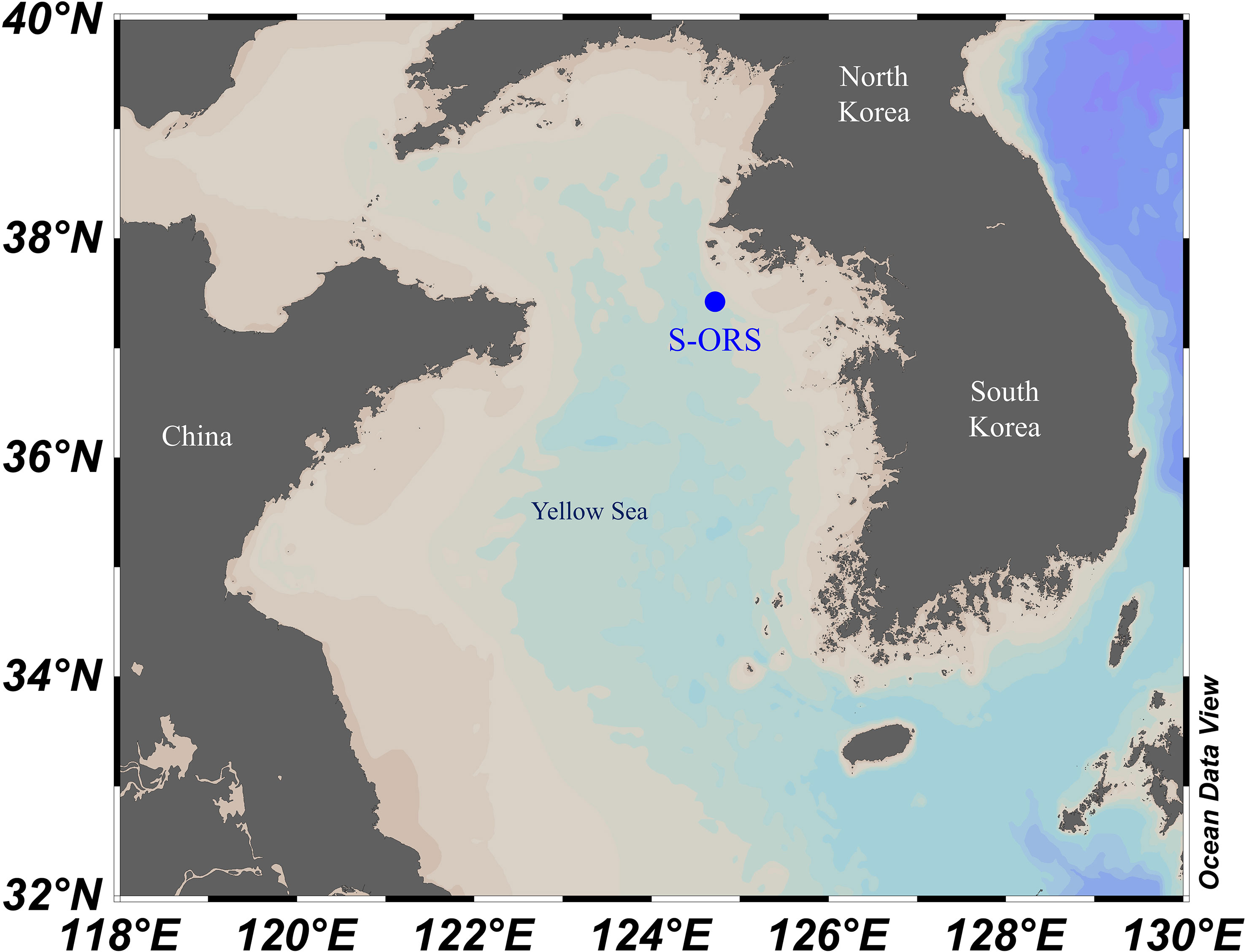
Figure 1 Location of the Socheongcho Ocean Research Station (S-ORS; blue dot).

FIGURE 2

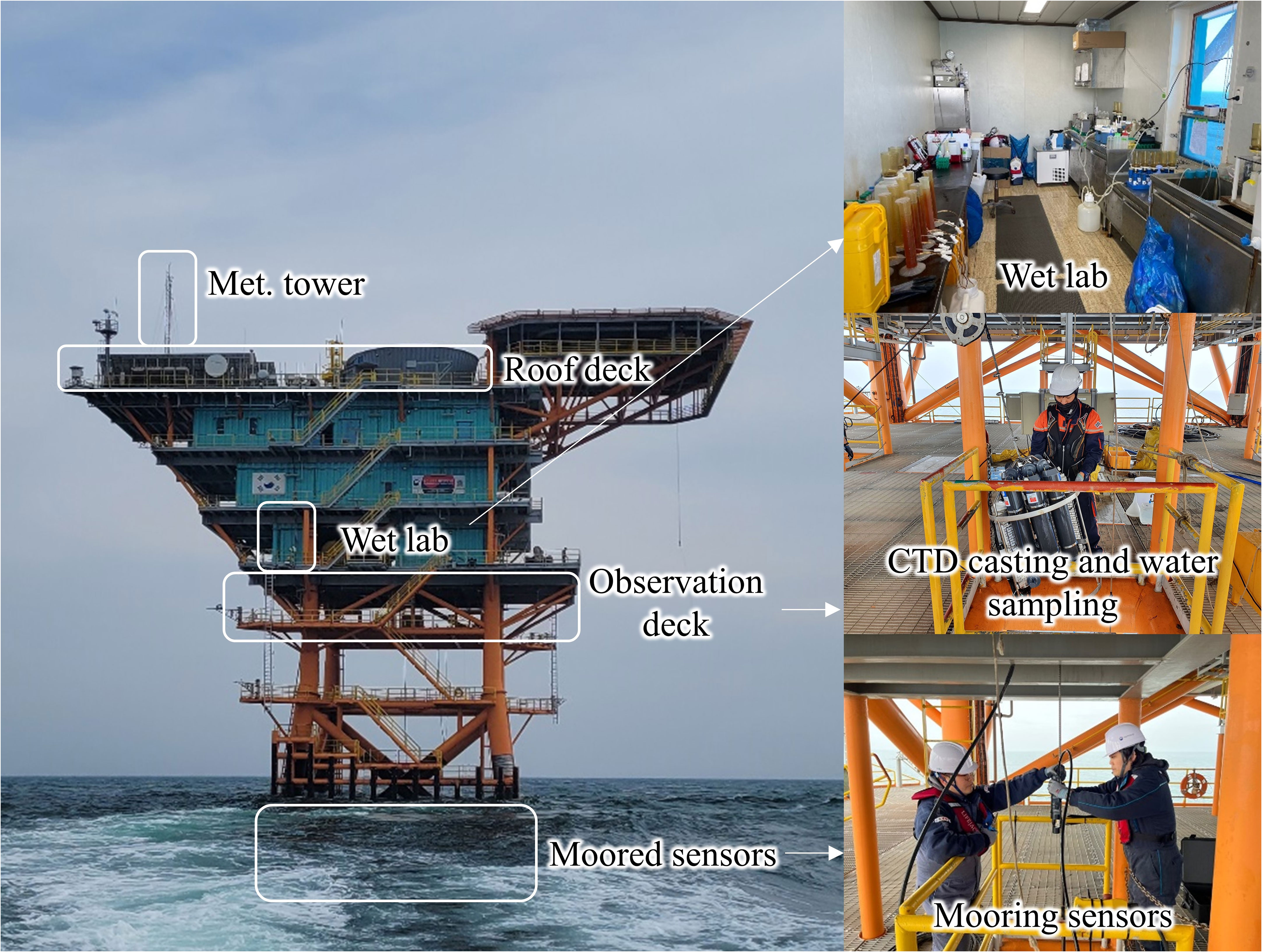
Figure 2 Images of S-ORS, including observation facilities used in this research.

TABLE 1

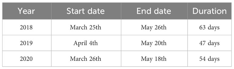
Table 1 Start and end dates of sample collection during each year.

2.2 Sample collection

Seawater was collected daily using a rosette sampler attached to a CTD recorder (SBE 19plus V2; Sea-Bird Scientific, Bellevue, WA, USA), except when unavoidable issues such as extreme weather conditions prevented sampling. We generally collected water samples at five depths: 0, 10, 20, 30, and 40 m. However, the sampling depths were slightly modified to include the sub-surface chlorophyll maximum (SCM) layer if present. Identification of the SCM was conducted using a fluorescence sensor equipped on the CTD. This process was conducted during daylight hours at low tide to account for the significant tidal ranges found in the Yellow Sea.

After obtaining the water sample, we followed appropriate methods to collect pigment and nutrient samples. First, we filtered 1 L of seawater through GF/F filters (Whatman PLC, Maidstone, UK) and then collected the filter paper for pigment sampling, while the filtrate was collected for dissolved inorganic nutrients. All samples were stored in a deep freezer on site and then transported on dry ice to the laboratory, where they were stored in another deep freezer until analysis.

2.3 Determination of pigment concentrations using high-performance liquid chromatography

The process of measuring pigment concentrations was described by Hyun et al. (2022), and we followed their detailed procedure. To maximize extraction efficiency, the filter papers were freeze-dried prior to extraction, soaked in 4 ml of an aqueous acetone solution (5:95 v:v), wrapped with aluminum foil to prevent exposure to light, and stored in a refrigerator at 4°C for 24 hours. The extracts were filtered again using 0.2-µm polytetrafluoroethylene syringe filters (Hyundai Micro, Seoul, Korea) to remove particles that may damage the HPLC system. After filtration, 1 ml of each filtrate was transferred into brown amber vials and 400 µl of HPLC-grade water was added.

The pigments were separated and measured using an HPLC system (LC-2030c 3D; Shimadzu Corporation, Kyoto, Japan) following a modified version of the protocol described by Zapata et al. (2000). Specifically, the separation of pigments was performed through reverse-phase chromatography using a C8 column (150 × 4.6 mm, 3.5 µm particle size, 100 Å pore size; Waters Corporation, Milford, MA, USA). The concentrations of the separated pigments were measured using the 440-nm chromatogram detected with a photodiode-array detector. Additionally, the purity of each peak was confirmed through measurement of wavelengths from 370 to 800 nm.

The factors used to convert peak area to pigment concentrations were determined on an annual basis prior to analysis when the C8 column was replaced for maintenance. This process involved analysis of standard pigments (DHI LAB, Hørsholm, Denmark) and the generation of a calibration curve. Additionally, to facilitate peak identification, a mixture of standard pigments was evaluated (first and last samples daily) during HPLC operation.

2.4 Chemotaxonomic analysis

The processes used to determine the Chl-a concentration and composition for each taxonomic group were conducted using CHEMTAX software (version 1.95) and the Bayesian Compositional Estimator (BCE) tool. In chemotaxonomic analysis, the inclusion of either too many or too few taxa can introduce substantial error into the results. To mitigate this possible source of error, taxa included in the calculation were carefully selected based on the examination of corresponding next-generation sequencing (NGS) data. The method used for NGS analysis strictly adhered to the procedures outlined by Choi et al. (2016); Yang et al. (2021), and Hyun et al. (2022).

Although the selection of taxa is an important aspect of chemotaxonomic analysis, the statistical methods used also have inherent limitations. CHEMTAX is underdetermined, which can introduce bias (Latasa, 2007; Van den Meersche et al., 2008), whereas BCE has issues with reproducibility (Hyun et al., 2022). Therefore, this study utilizes a combination of these methods to address these issues: the underdetermined bias of CHEMTAX can be dealt with by constraining the pigment ratio variation range (Hyun et al., 2022), while BCE is appropriate for obtaining a range of coefficients rather than exact coefficient values. Therefore, we first determined the pigment variation range using BCE; the initial ratios and ratio limit matrices (RLMs) were obtained based on that range. Finally, CHEMTAX analysis was conducted with the initial ratios and RLMs to assess taxonomic composition.

Prior to the CHEMTAX analysis, the samples were pre-clustered based on sampling date into 14 clusters. This process was used to prevent decreased precision of both CHEMTAX and BCE analyses caused by the inclusion of too many samples in a single run. BCE analysis was conducted using the BCE package (Van den Meersche and Soetaert, 2022) in the R programming language (R Core Team, 2022). The starting pigment ratio was obtained by reconstructing the pigment ratio statistics of Roy et al. (2011), and is presented in Supplementary Table S1.

For each cluster, 100,000 iterations were conducted with a burn-in length of 35,000. An updated covariance value of 100 was applied, and the jump length was finely adjusted separately for each cluster to avoid autocorrelation in the trace plot and achieve an acceptance rate of 30–80%. Detailed information about the pre-clustering, adjusted jump length, and resulting acceptance rate for each cluster is provided in Supplementary Table S2. For settings that are not listed in the Supplementary Material, we used the defaults provided in the BCE package.

The initial ratios and RLMs used for CHEMTAX analysis were based on the 99% confidence intervals produced by the BCE analysis of pigment ratios. CHEMTAX analysis was conducted with the following settings, which were adapted from Latasa (2007): iteration limit of 5,000, epsilon limit of 0.0001, initial step size of 25, step ratio of 2, cutoff of 30,000, and bounded relative weighting.

To visualize the station location and results, which include Chl-a concentrations for each phytoplankton group, CTD, and nutrient data, we used the Ocean Data View software (Schlitzer, 2022).

2.5 Environmental factors associated with vertical mixing

Wind speed, wave height, atmospheric temperature, and sea surface temperature (SST) data were collected by sensors equipped on S-ORS. Specific details of the equipment are presented in Supplementary Table S3. The locations of sensors in S-ORS are depicted in Figure 2.

Wind speed, atmospheric temperature, and SST data were collected on a minute-by-minute basis, then averaged to obtain daily average values. Significant wave height was continuously calculated throughout each day, rather than averaged.

The stratification, MLD, pycnocline depth, and density gradient of the pycnocline were calculated based on the vertical CTD profile for each day. Water column stratification was determined as the sigma-t difference between the bottom (at 40 m) and surface waters. The MLD was defined as the shallowest depth at which sigma-t exceeds the surface value by more than 0.03 kg/m³ (de Boyer Montégut et al., 2004). Because of CTD instrument instability near the surface, we used the value at 5 m as a proxy for surface density. The density gradient was determined as the density difference relative to the depth 1 m above, and the pycnocline was defined as the depth with the maximum density gradient on a particular day.

Pearson’s correlation-based network analysis was conducted between Chl-a and the parameters associated with vertical mixing to examine how those factors influence the spring bloom process. For this network analysis, data collected after the Chl-a peak were excluded to focus on the bloom formation process, rather than the bloom decrease process.

2.6 Multivariate analysis and time-series analysis

To elucidate the process through which environmental variables affect the biomass of each phytoplankton group, multivariate analysis to explain the patterns is needed. Statistical analysis was conducted using the R programming language (R Core Team, 2022). RDA was performed to identify significant distribution patterns of phytoplankton group biomass in relation to environmental factors. This analysis was conducted using the Vegan package (version 2.6-2) (Simpson et al., 2022).

Time-series analysis was conducted to address time-dependent mechanisms that are difficult to explain with RDA. DFA was performed on surface water samples using the MARSS package (Holmes et al., 2012; Holmes et al., 2021a; Holmes et al., 2021b) and the results were visualized using the ggplot2 package (Wickham, 2016). For the DFA model, we established the observation equation [Equation (1)] and state space equation [Equation (2)]:

$\begin{array}{ll}{y}_t=\text{Γ}{\alpha }_t+\mu +D{x}_t+{\epsilon }_t& (1)\end{array}$

$\begin{array}{ll}{\alpha }_t={\alpha }_{t-1}+{\eta }_t& (2)\end{array}$

where $y_t$ represents the phytoplankton biomass of each group at time t, formatted as a 6 × n matrix in which rows represent the six phytoplankton groups analyzed with CHEMTAX, while columns represent samples. α represents the state value, which is a latent factor influencing the observed variables; it is a 5 × n matrix because we included five state space variables. Γ represents the factor loadings that link the observed variables to the state space, and is a 6 × 5 matrix. µ indicates the intercept, and $x$ represents the five covariates included in the model: temperature, salinity, nitrate, phosphate, and silicate. D represents factor loadings linking the covariates with the observed variable. ϵ and η are error terms for the observation and state space, respectively. For ϵ, an optimized diagonal and unequal matrix is used, while for η an identity matrix is employed.

The number of state spaces is determined by comparing the corrected Akaike information criterion (AICc) for one to five state spaces and selecting the smallest AICc, which was obtained with five state spaces. To identify covariates to include in the model, we tested multiple physical and chemical environmental variables, including the nitrogen to phosphorus (NP) ratio. Through the comparison of AICc values, we selected five covariates. To prevent the model from being underdetermined, we constrained some elements of the Γ, µ, and D matrices. The designs for these matrices are shown in (3). ${\gamma }_{i,j},a_i,d_{i,j}$ are the parameters calculated by the model, while the 0 values remain unmodified.

$\begin{array}{ll}\text{Γ}=\left[\begin{array}{lllll}{\gamma }_{11}\hfill & 0\hfill & 0\hfill & 0\hfill & 0\hfill \\ {\gamma }_{21}\hfill & {\gamma }_{22}\hfill & 0\hfill & 0\hfill & 0\hfill \\ {\gamma }_{31}\hfill & {\gamma }_{32}\hfill & {\gamma }_{33}\hfill & 0\hfill & 0\hfill \\ {\gamma }_{41}\hfill & {\gamma }_{42}\hfill & {\gamma }_{43}\hfill & {\gamma }_{44}\hfill & 0\hfill \\ {\gamma }_{51}\hfill & {\gamma }_{52}\hfill & {\gamma }_{53}\hfill & {\gamma }_{54}\hfill & {\gamma }_{55}\hfill \\ {\gamma }_{61}\hfill & {\gamma }_{62}\hfill & {\gamma }_{63}\hfill & {\gamma }_{64}\hfill & {\gamma }_{65}\hfill \end{array}\right],\mu =\left[\begin{array}{l}0\hfill \\ 0\hfill \\ 0\hfill \\ 0\hfill \\ 0\hfill \\ a_6\hfill \end{array}\right],D=\left[\begin{array}{lllll}{d}_{11}\hfill & d_{12}\hfill & d_{13}\hfill & d_{14}\hfill & d_{15}\hfill \\ d_{21}\hfill & d_{22}\hfill & d_{23}\hfill & d_{24}\hfill & d_{25}\hfill \\ d_{31}\hfill & d_{32}\hfill & d_{33}\hfill & d_{34}\hfill & d_{35}\hfill \\ d_{41}\hfill & d_{42}\hfill & d_{43}\hfill & d_{44}\hfill & d_{45}\hfill \\ d_{51}\hfill & d_{52}\hfill & d_{53}\hfill & d_{54}\hfill & d_{55}\hfill \\ d_{61}\hfill & d_{62}\hfill & d_{63}\hfill & d_{64}\hfill & d_{65}\hfill \end{array}\right]& (3)\end{array}$

3 Results

3.1 Physical characteristics

The physical characteristics of the water column during the spring research periods of 2018, 2019, and 2020 were investigated in this study (Figure 3). The temperature of the water during the 2018 sampling period ranged from 4.43 to 15.10°C, with a steady increase over time. Initially, no significant temperature differences were observed with depth. However, the surface temperature increased rapidly, resulting in the development of a thermocline in late April that persisted around a depth of 15 m for most of May. The 2019 research period exhibited a similar pattern, with a water temperature ranging from 6.45 to 15.76°C and a thermocline forming at a shallower depth of around 10 m. In contrast, the 2020 season displayed significant differences, with a much narrower temperature range between 6.78 and 11.32°C and a shallow thermocline that developed only toward the end of the research period.

FIGURE 3

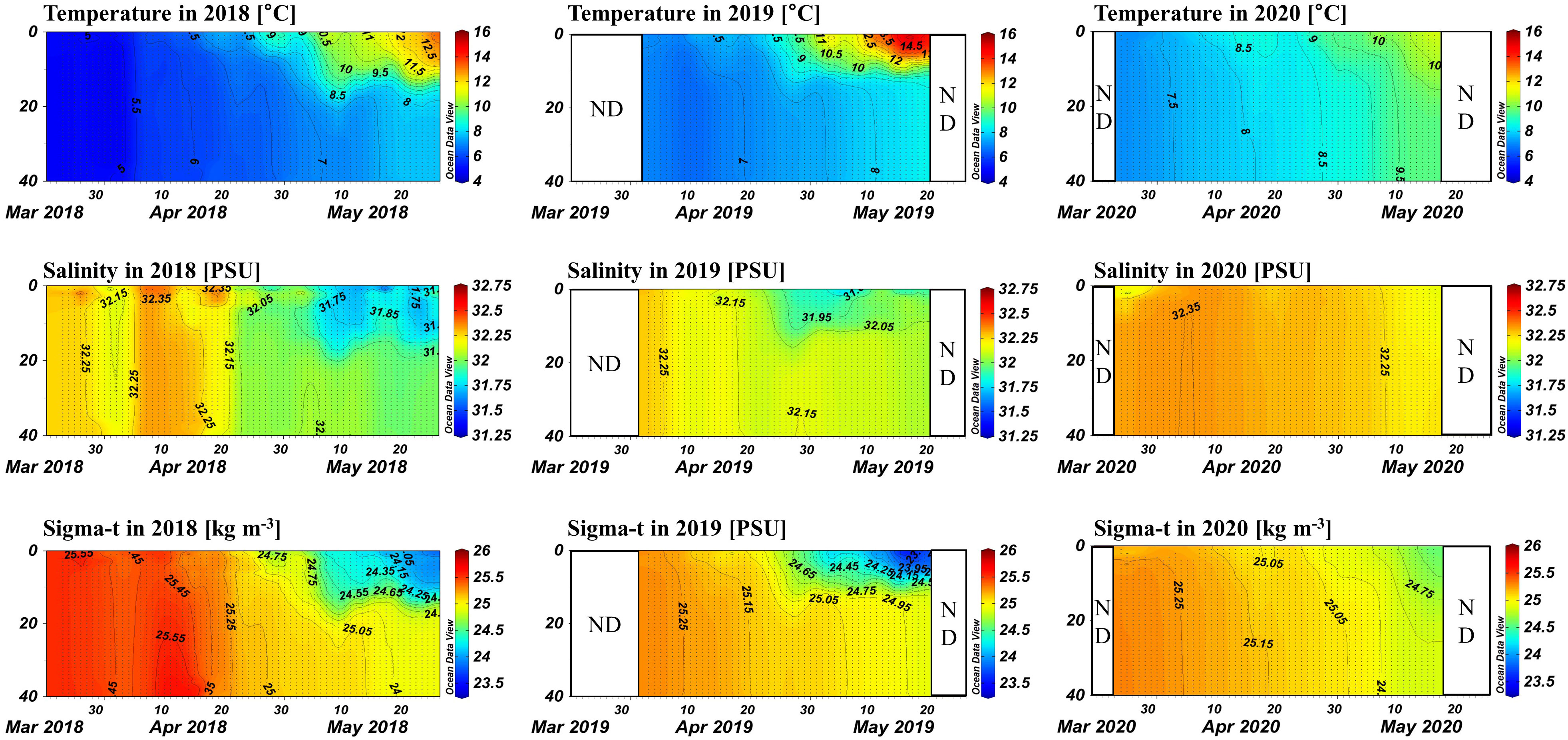
Figure 3 Contour plots of temperature, salinity, and density for each year. The x-axis represents time (days), and the y-axis represents water depth (m).

During the 2018 and 2019 research periods, salinity showed decreasing trends, ranging from 31.136 to 32.632 PSU and 31.647 to 32.313 PSU, respectively. However, the 2020 research period exhibited a distinct trend, with salinity remaining relatively constant between 32.086 and 32.405 PSU throughout the study period.

In early spring of 2018 and 2019, when sampling began, no significant density differences were found, indicating a well-mixed environment at the start of sampling.

The pycnocline began to form in late April and persisted until the end of the research period. In contrast, during 2020, the pycnocline was not well developed until the end of the study period, allowing for greater vertical mixing.

The temperature–salinity (T-S) diagram presented in Figure 4 provides a clear representation of the observed trend. Salinity was highest in 2020, followed by 2019 and then by 2018. However, potential temperature, rather than salinity, was the primary driver of the observed vertical density differences. In 2018, potential temperature was lowest during the early spring season and gradually increased over time, thereby contributing to the observed vertical density difference. Potential temperature increased more rapidly in 2019, resulting in a vertical density difference similar to that observed in 2018. The trend in 2020 differed significantly, with potential temperature being highest at the start of the research period and surface potential temperature being lowest at the end of the study period among the 3 years, resulting in a relatively small vertical density difference.

FIGURE 4

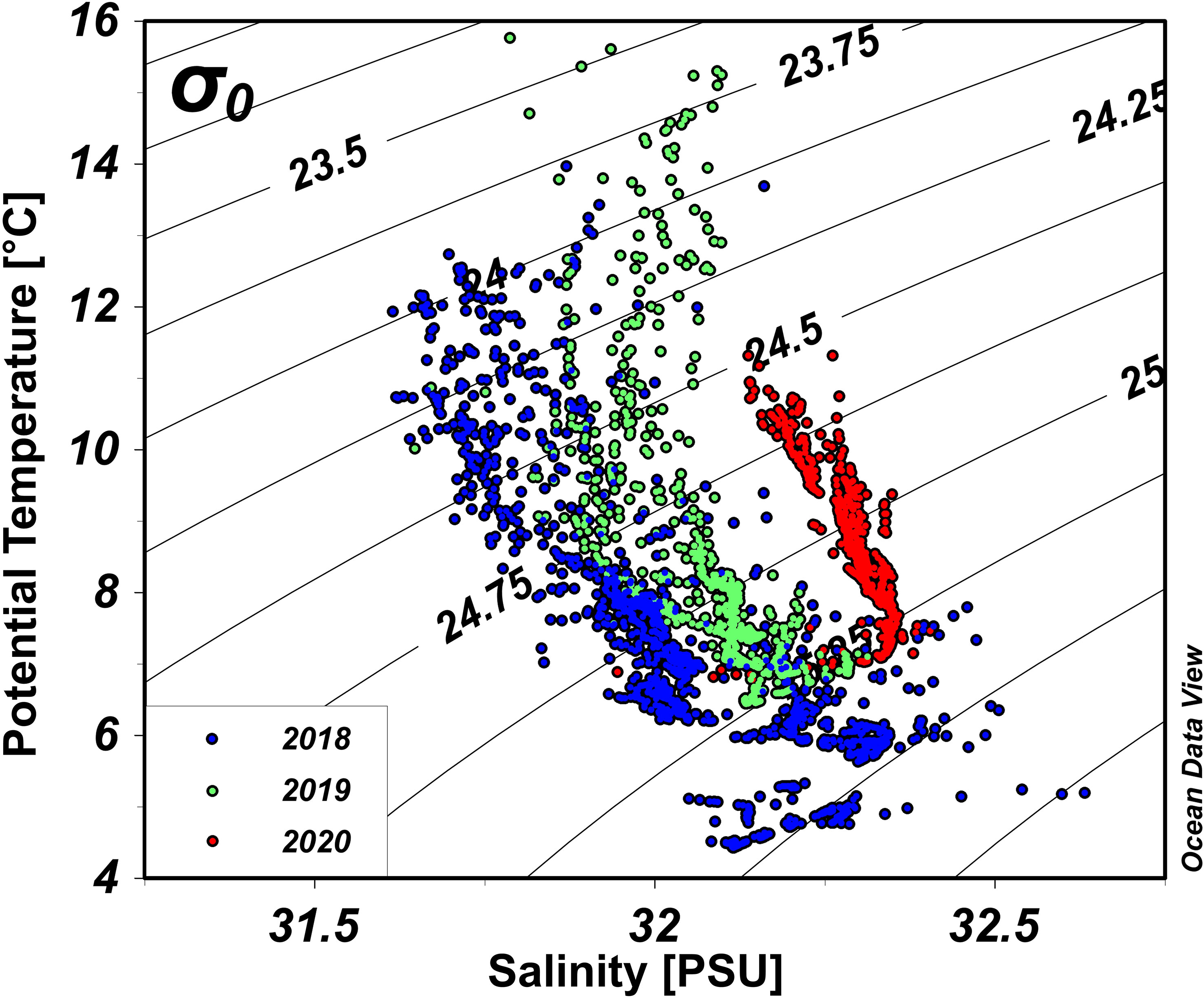
Figure 4 Temperature–salinity diagram for 1-m bin-averaged conductivity-temperature-depth (CTD) data for all dates. Blue, green, and red dots represent data from 2018, 2019, and 2020, respectively.

3.2 Distributions of inorganic nutrients

The concentrations of nitrate, phosphate, and silicates, which are major inorganic nutrients utilized by marine primary producers, exhibited a common pattern of high levels in early spring followed by steady decreases ~ over time (Figure 5). The rate of decrease in nutrient concentrations was highest above the pycnocline, especially for phosphate, resulting in an increase in the NP ratio of surface water after pycnocline formation and indicating phosphate limitation in the upper water column. In 2020, no significant pycnocline formed, resulting in a more uniform nutrient pattern throughout the water column, which may have impacted the phytoplankton community.

FIGURE 5

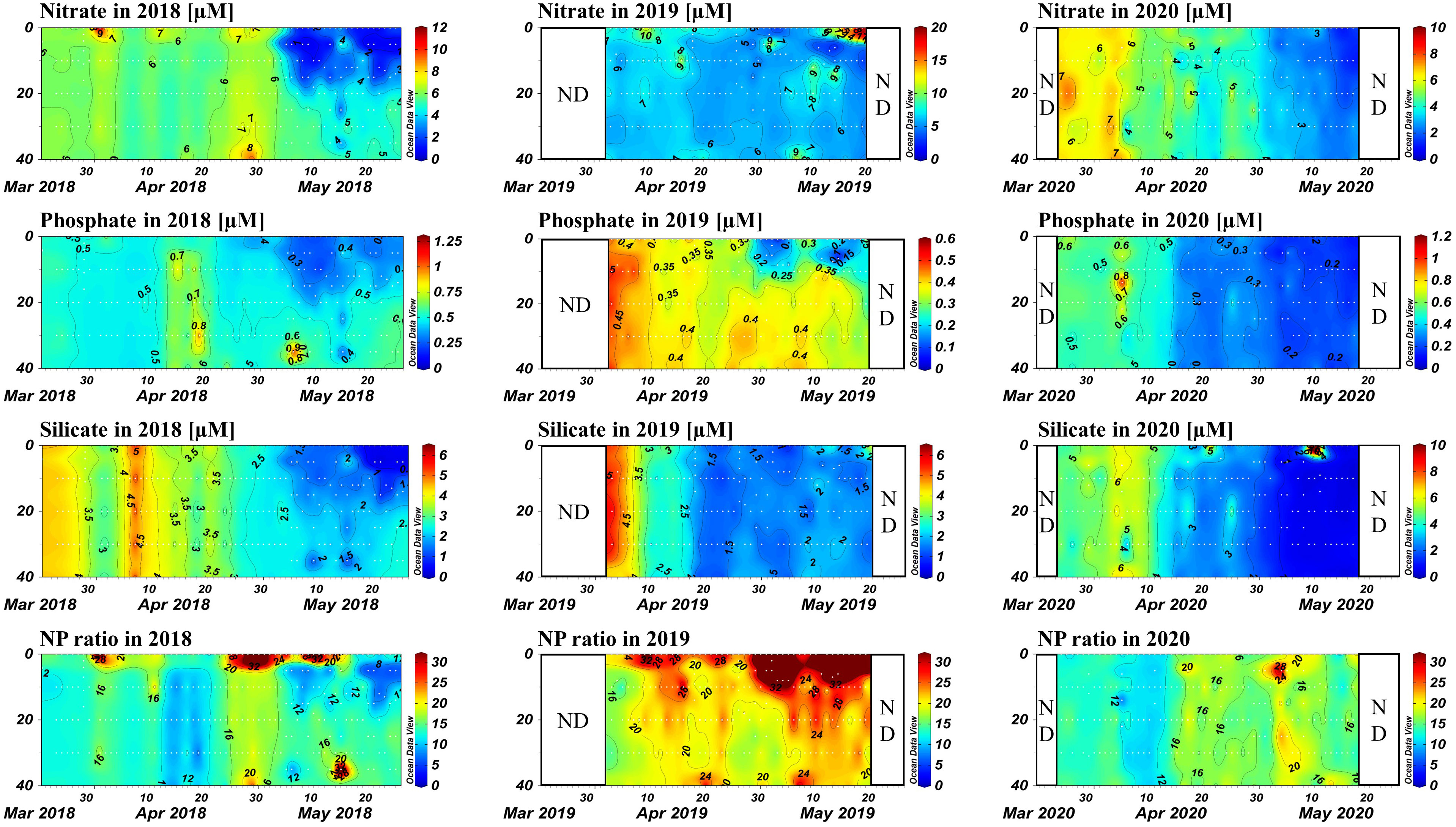
Figure 5 Contour plots of nitrate, phosphate, and silicate concentrations, and NP ratios, for each year. The x-axis represents time (days), and the y-axis represents depth.

During early spring of 2018, which had the lowest water temperature among the 3 years studied, nutrient concentrations exhibited fluctuations rather than a steady decrease. The concentration of nitrate ranged between 4.85 and 8.30 µM, that of phosphate ranged between 0.44 and 0.93 µM, and that of silicate ranged between 2.64 and 6.39 µM prior to 20 April. Subsequently, nutrient concentrations decreased significantly, particularly in surface waters, with the concentration of nitrate ranging between 0.52 and 10.83 µM, that of phosphate ranging between 0.16 and 1.24 µM, and that of silicate ranging between 0.21 and 4.18 µM until the end of the 2018 study period. Extreme values of the NP ratio (typically > 30 with a maximum value of 55.0) were observed in surface water between 26 April and 16 May as phosphate became limited. These extreme events occurred in surface waters only after the pycnocline formed, and the average NP ratio for the entire 2018 sampling period was 15.02 ± 6.82.

Among the years studied, 2019 had the lowest phosphate concentrations, which showed a tendency to decrease shortly after the research period began. The concentration of nitrate fluctuated between 2.11 and 26.27 µM. The concentration of phosphate ranged between 0.02 and 0.57 µM, and that of silicate ranged between 0.25 and 5.91 µM. These concentrations resulted in high NP ratios, with an average of 26.98 ± 24.15. Extreme values were observed in surface waters, with a maximum of 225.68.

In 2020, a similar decreasing trend in nutrient concentrations was observed, with less significant vertical differences compared to the previous 2 years. The concentration of nitrate ranged between 0.60 and 8.37 µM, that of phosphate ranged between 0.06 and 1.28 µM, and that of silicate ranged between 0.12 and 10.60 µM. The average NP ratio during this season was 18.55 ± 14.85, and no extreme values were observed in surface water.

The NP ratios were generally distributed near the 16:1 line, with only a few outliers (Figure 6). Extremely high NP ratios were typically observed in surface waters after pycnocline formation, but no clear distributional trend of extremely low ratios was observed. Furthermore, most data from 2019 fell above the 16:1 line, indicating an overall pattern of phosphate limitation during that year.

FIGURE 6

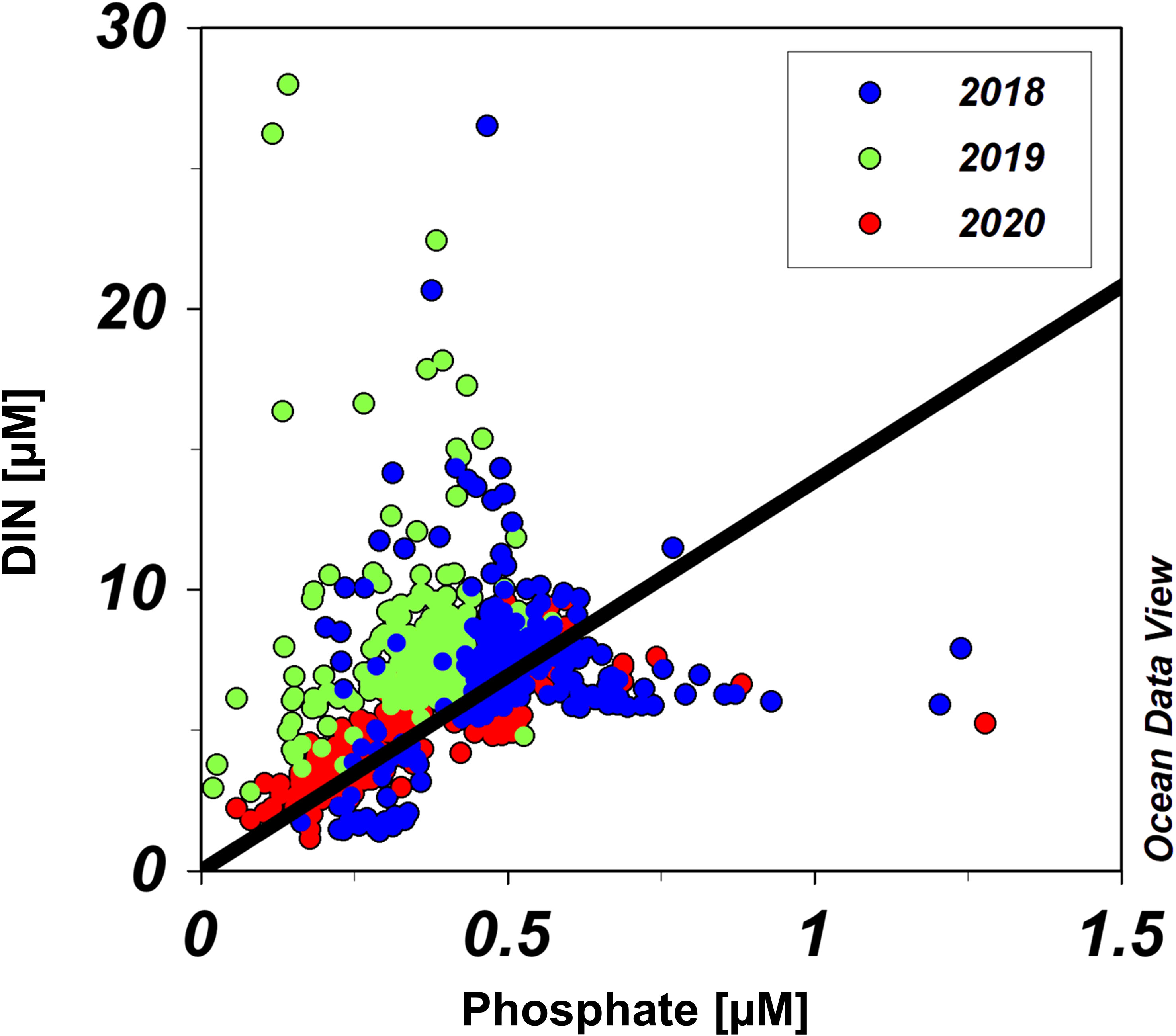
Figure 6 Nitrogen to phosphorus (NP) ratios for all samples. Blue, green, and red dots represent data from 2018, 2019, and 2020, respectively. Solid line is a 16:1 line.

3.3 Distributions of phytoplankton groups revealed through the chemotaxonomic approach

The Chl-a concentrations of the phytoplankton groups are shown in Figure 7. Throughout the 3-year study period, several common trends were observed. Bacillariophyceae and Cryptophyceae were the dominant phytoplankton groups throughout the study, with their biomass increasing as concentrations of nutrients, particularly phosphate, decreased throughout the water column in the early period. As the pycnocline developed, large increases in chlorophytes and cryptophytes were observed near the water surface, while the biomass of Bacillariophyceae decreased throughout the water column, as did the that of Cryptophyceae below the pycnocline. Slight increases in Prymnesiophyceae and Dinophyceae occurred above the pycnocline just after the chlorophyte bloom. Synechococcus exhibited an overall pattern similar to that of Bacillariophyceae, although it had much lower biomass than the other groups. Table 2 provides the average concentrations and concentration ranges of Chl-a for each group and year.

FIGURE 7

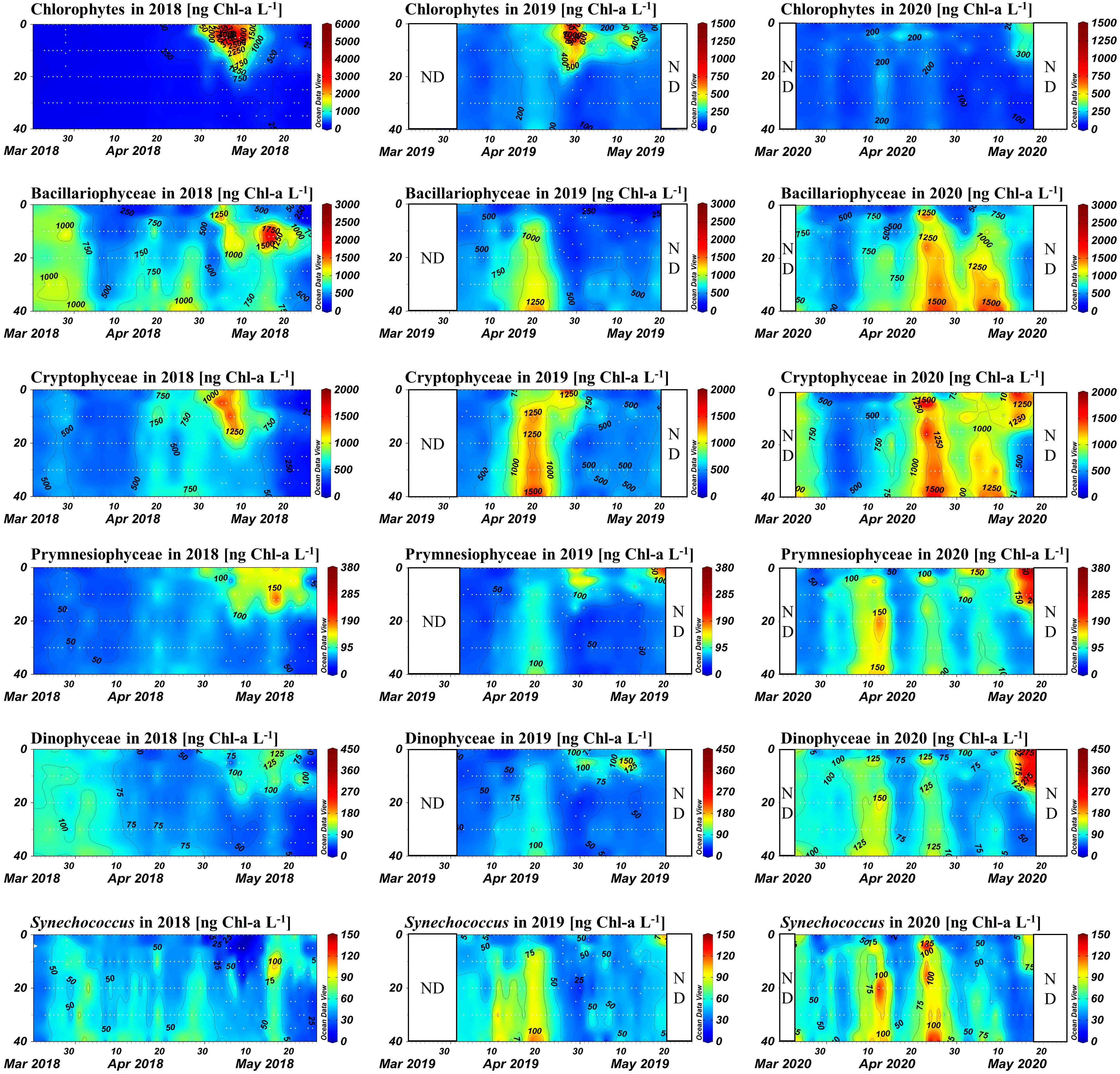
Figure 7 Contour plots of Chl-a concentrations for each phytoplankton group, for each year, calculated by chemotaxonomic analysis. The x-axis represents time (days), and the y-axis represents water depth (m). Consistent scales are used where possible for ease of comparison; however, the 2018 chlorophyte bloom necessitated a unique scale.

TABLE 2

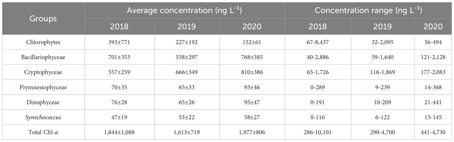
Table 2 Average concentrations and concentration ranges of chlorophyll a (Chl-a) for each phytoplankton group and year.

In the early spring period of 2018, Bacillariophyceae was the dominant group; its biomass showed the opposite trend to the nutrient concentrations, particularly phosphate. This finding suggests that during the early spring season, the top-down effect outweighed the bottom-up effect (i.e., phytoplankton uptake controlled nutrient levels). After the pycnocline developed, the biomass of Bacillariophyceae was rapidly replaced with chlorophytes in the surface water. On 7 May, the peak of the bloom, chlorophytes contributed 8,437 ng L⁻¹ of the total of 10,101 ng L⁻¹ Chl-a; Bacillariophyceae accounted for only 700 ng L⁻¹ in the same sample. Above the pycnocline, cryptophytes were the second most abundant group during this period. Thereafter, the biomass of Prymnesiophyceae and Dinophyceae increased, while the three major groups decreased simultaneously above the pycnocline. Despite the increase, the biomass of Prymnesiophyceae and Dinophyceae did not exceed that of the three major groups.

In 2019, at the beginning of the research period, Bacillariophyceae and Cryptophyceae were the two major groups, in accordance with 2018. The biomass of these two taxa increased throughout the water column as levels of phosphate and silicate decreased, and this increase continued until the pycnocline began to develop. One difference in this trend from 2018 is that the biomass of all other groups increased simultaneously. The surface chlorophyte and Cryptophyceae bloom occurred after the pycnocline had developed, but its scale was much smaller than in 2018; 2,095 ng L⁻¹ Chl-a was derived from chlorophytes, and 1,869 ng L⁻¹ from Cryptophyceae, out of the total 4,700 ng L⁻¹ Chl-a. After that period, a slight increase in Prymnesiophyceae and Dinophyceae biomass was observed, as in 2018, but the extent and duration of these increases were smaller.

During 2020, no bloom of chlorophytes and Cryptophyceae in the surface water was observed, as the pycnocline was not present during the 2020 research period. Instead, high levels of Bacillariophyceae and Cryptophyceae biomass persisted longer throughout the water column compared to the other 5 years. Consequently, the maximum Chl-a value during 2020 was observed in the bottom water (40 m) on 27 April, whereas in the other two years the maximum value occurred in the surface water during the extreme biomass increase of the chlorophytes; of the 4,730 ng L⁻¹ of Chl-a, 2,090 ng L⁻¹ was from Bacillariophyceae and 1,959 ng L⁻¹ was from Cryptophyceae. Around 15 May, a surface Chl-a increase was detected as the pycnocline began to form, which was much later than in the other 2 years studied. However, the extent of this increase was smaller (maximum value, 3,590 ng L⁻¹ Chl-a), as the available nutrients had been consumed by Bacillariophyceae and Cryptophyceae. Instead of chlorophytes and Cryptophyceae accounting for most of the biomass, all groups excluding Bacillariophyceae increased simultaneously.

3.4 Relationships among vertical mixing parameters and resulting nutrients and phytoplankton Chl-a concentrations in each taxonomic group

Network analysis was conducted between the parameters associated with vertical mixing and the resulting nutrient and Chl-a concentrations for each phytoplankton group. For this analysis, only surface data prior to the Chl-a peak were included to focus on the bloom formation process. Table 3 presents Pearson’s correlation coefficients (r) between Chl-a and each variable. Additional network analysis was conducted to investigate interrelationships among variables (Figure 8). Only correlations with r< −0.45 or r > 0.45 were included in the network analysis plot.

TABLE 3

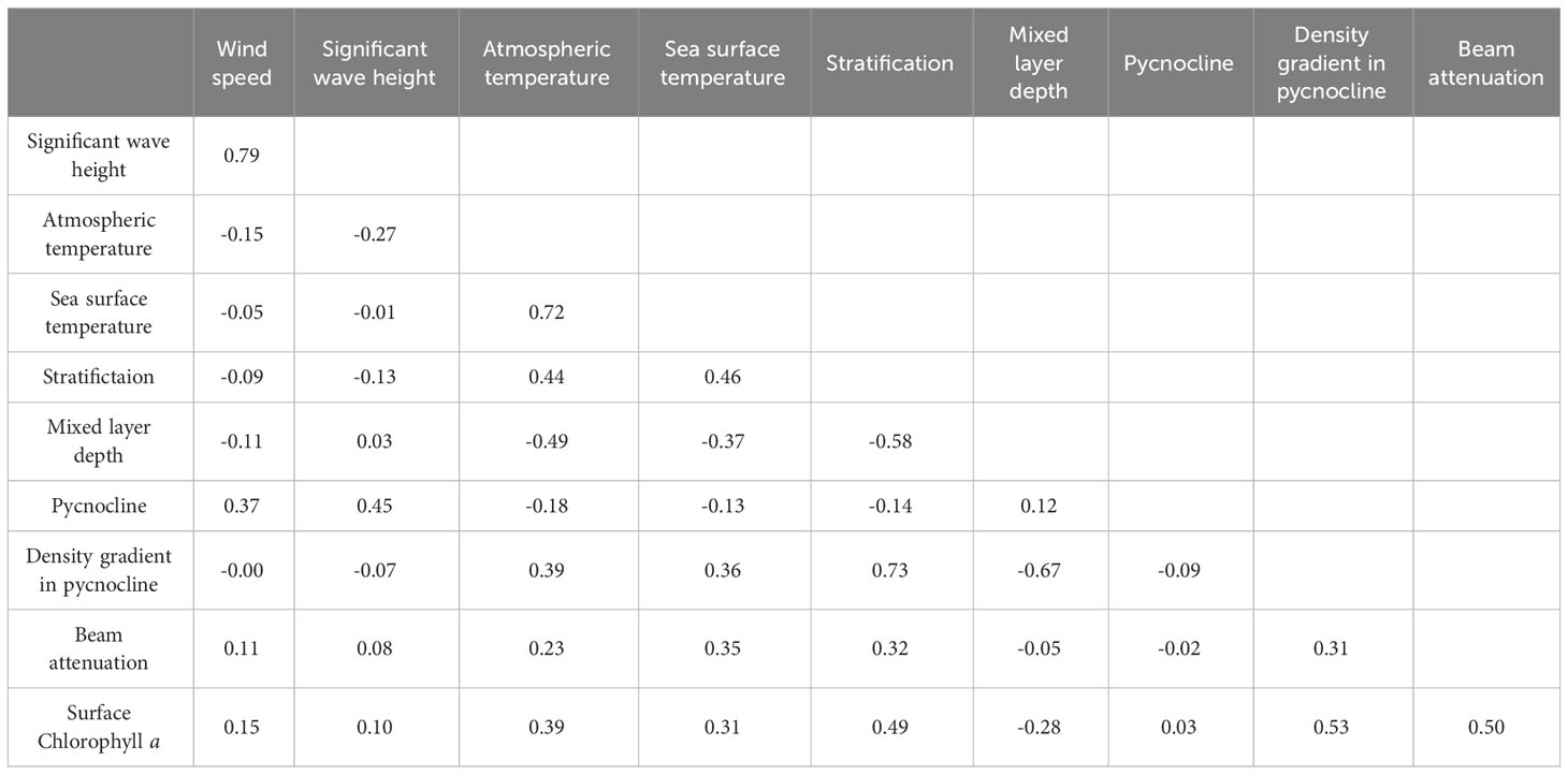
Table 3 Pearson’s correlation coefficients between vertical mixing-related environmental factors and surface Chl-a concentrations.

FIGURE 8

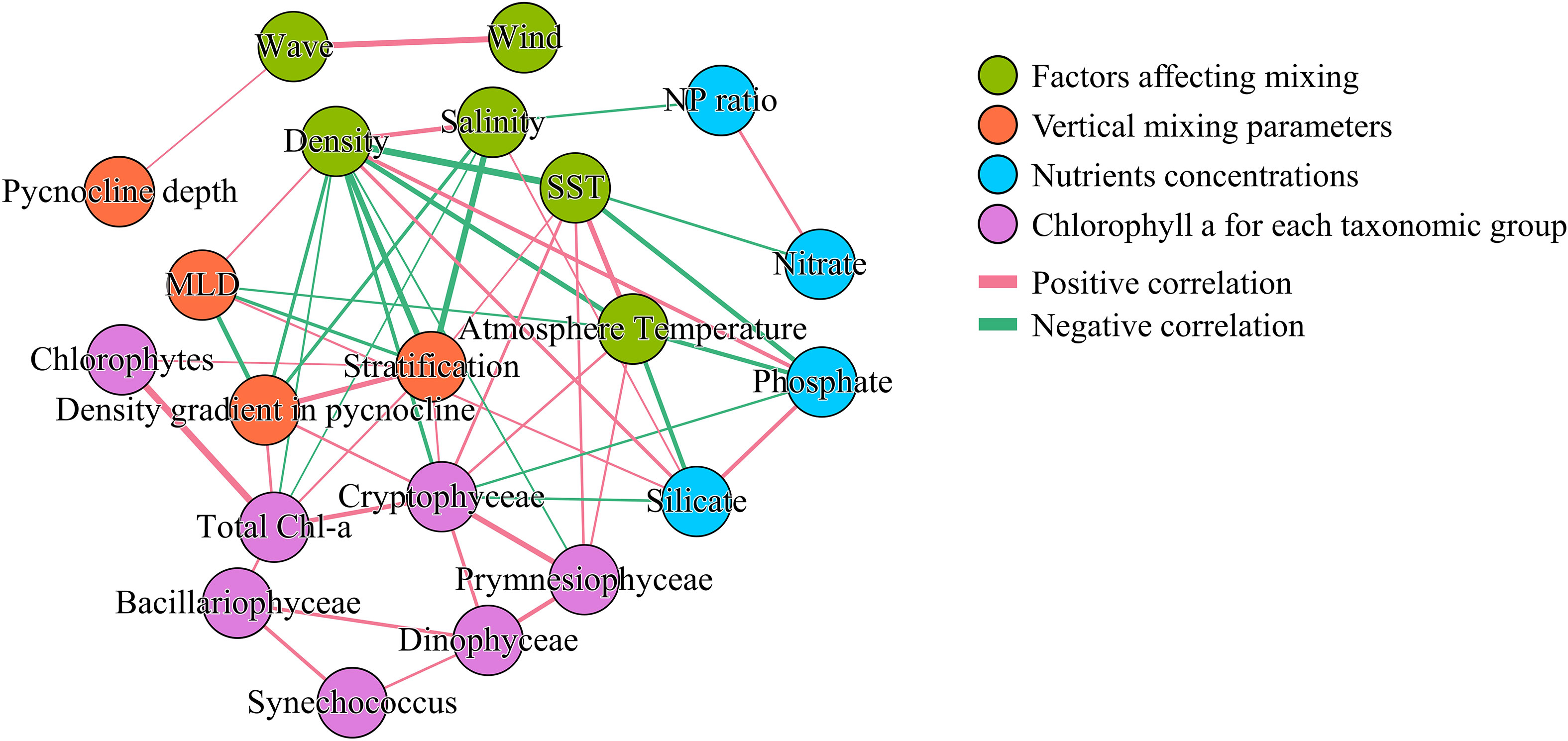
Figure 8 Network analysis of surface Chl-a concentrations for each phytoplankton group and variables related to vertical mixing, based on Pearson’s correlation analysis, assessed using correlation coefficients (r). Only relationships with r< −0.45 or r > 0.45 are shown. Edge thickness indicates correlation strength.

Among the factors influencing mixing, wave height and wind were strongly correlated with each other (r = 0.79), but were rarely linked with other variables, the sole exception being the correlation between pycnocline depth and wave height (r = 0.45). In contrast, atmospheric and sea surface temperatures (SSTs) were related to seven other nodes spanning multiple categories. However, only two edges connected vertical mixing parameters with these two temperatures: one between MLD and atmospheric temperature and another between stratification and SST. Surface density, which had the most connections, was related to three factors affecting mixing, three vertical mixing parameters, two nutrient factors, and Chl-a content of one specific taxonomic group.

Total Chl-a was linked with density, stratification, salinity, and the density gradient in the pycnocline. However, when segmented into groups, Chlorophytes correlated solely with stratification, while Cryptophyceae associated with seven factors, excluding the biomass of other taxonomic groups. The Bacillariophyceae, which is one of the main group for the spring S-ORS only shows the correlation between other taxonomic groups but the other environment factors, while Prymnesiophyceae have connected with density, SST, and atmosphere temperature but not with vertical mixing or nutrients. Dinophyceae and Synechococcus each correlate with two specific phytoplankton groups but not connected with other environmental factors. Notably, the mixed layer depth does not have any connections with any phytoplankton group.

3.5 Multivariate analysis of phytoplankton Chl-a concentrations for each group and related environmental variables

To explore the relationship between phytoplankton community structure and key environmental variables, we performed RDA (Figure 9). Prior to the development of the pycnocline, when physical characteristics such as low temperature, high density, and elevated salinity were consistent, most of the sample data clustered near the center of the RDA1 axis. However, data points with higher temperatures, particularly those collected near the surface after the development of the pycnocline, shifted toward the first quadrant. The density gradient of the pycnocline emerged as a predominant factor explaining the variance in data points away from the surface. The placement of the data points appears to align with the directions of the variables. However, distinctions between years for data collected below the surface were not readily apparent on the triplot.

FIGURE 9

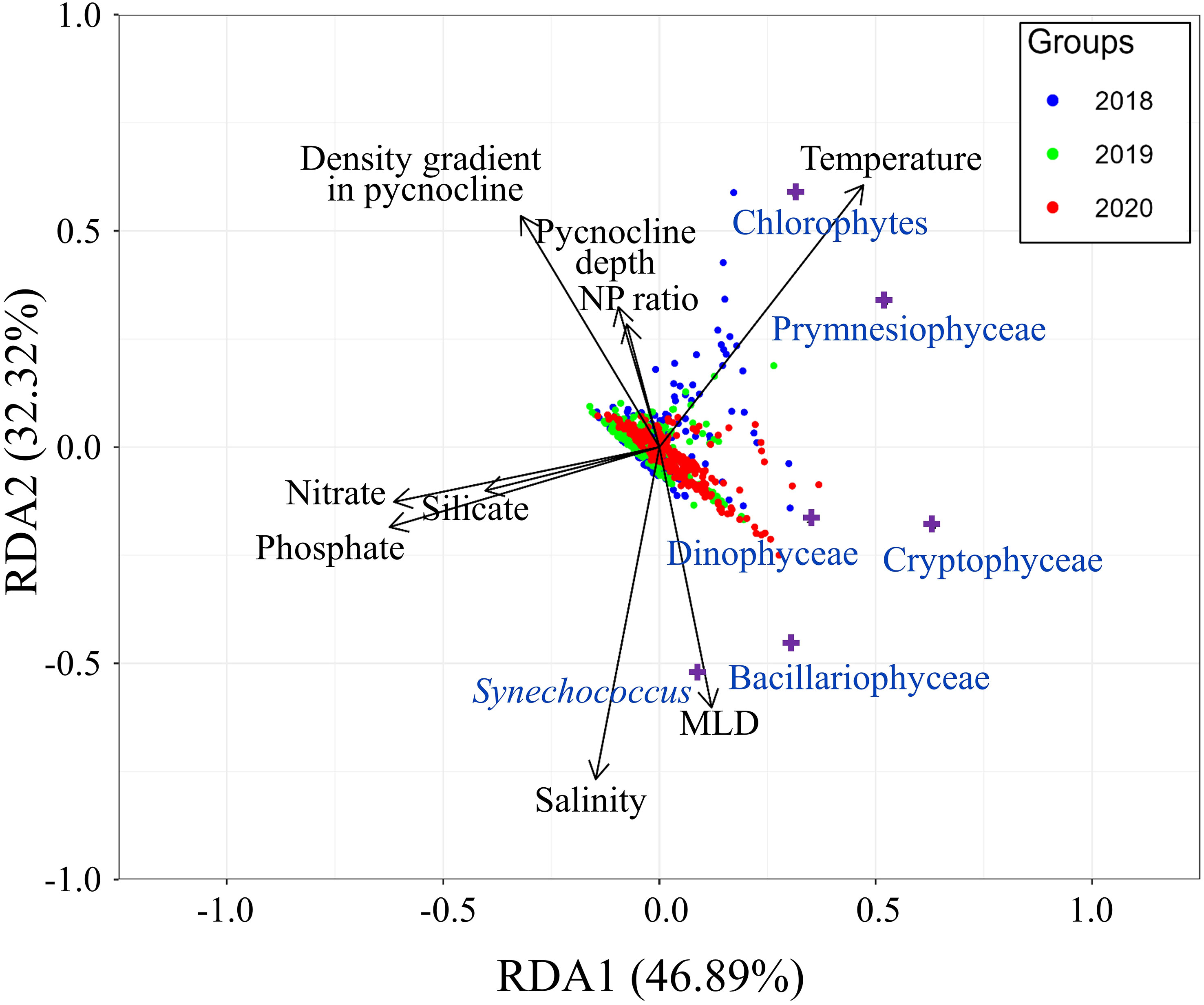
Figure 9 Redundancy analysis triplot illustrating relationships between phytoplankton community structure and major environmental variables. Blue, green, and red dots represent data from 2018, 2019, and 2020, respectively; purple crosses indicate phytoplankton groups.

With respect to phytoplankton groups, chlorophytes tended to be present at high levels when the temperature, pycnocline density gradient and NP ratio were high, and salinity was low. Prymnesiophyceae had high abundance when the temperature was high and nutrient concentrations were low. Bacillariophyceae and Cryptophyceae had high biomass when both the NP ratio and pycnocline density gradient were low. However, Cryptophyceae favored higher temperatures than Bacillariophyceae. Dinophyceae exhibited a preference for low pycnocline density gradient, but to a lesser extent than Bacillariphyceae and Cryptophyceae, and they thrived at intermediate nutrient and temperature levels. Synechococcus biomass appeared to increase at high salinity and MLD, along with a low NP ratio and pycnocline density gradient. However, the biomass of Synechococcus was too low for accurate determination of the trend in their distribution.

3.6 DFA of surface Chl-a for each group

RDA reveals the overall pattern of phytoplankton biomass across environmental gradients, but does not elucidate the mechanisms occurring throughout the study period. Therefore, we conducted time-series analysis to reveal these mechanisms. The DFA model was employed for this analysis. Figure 10 compares the actual and model-expected values. The overall trend accurately predict by model, with only minor discrepancies observed for extreme values.

FIGURE 10

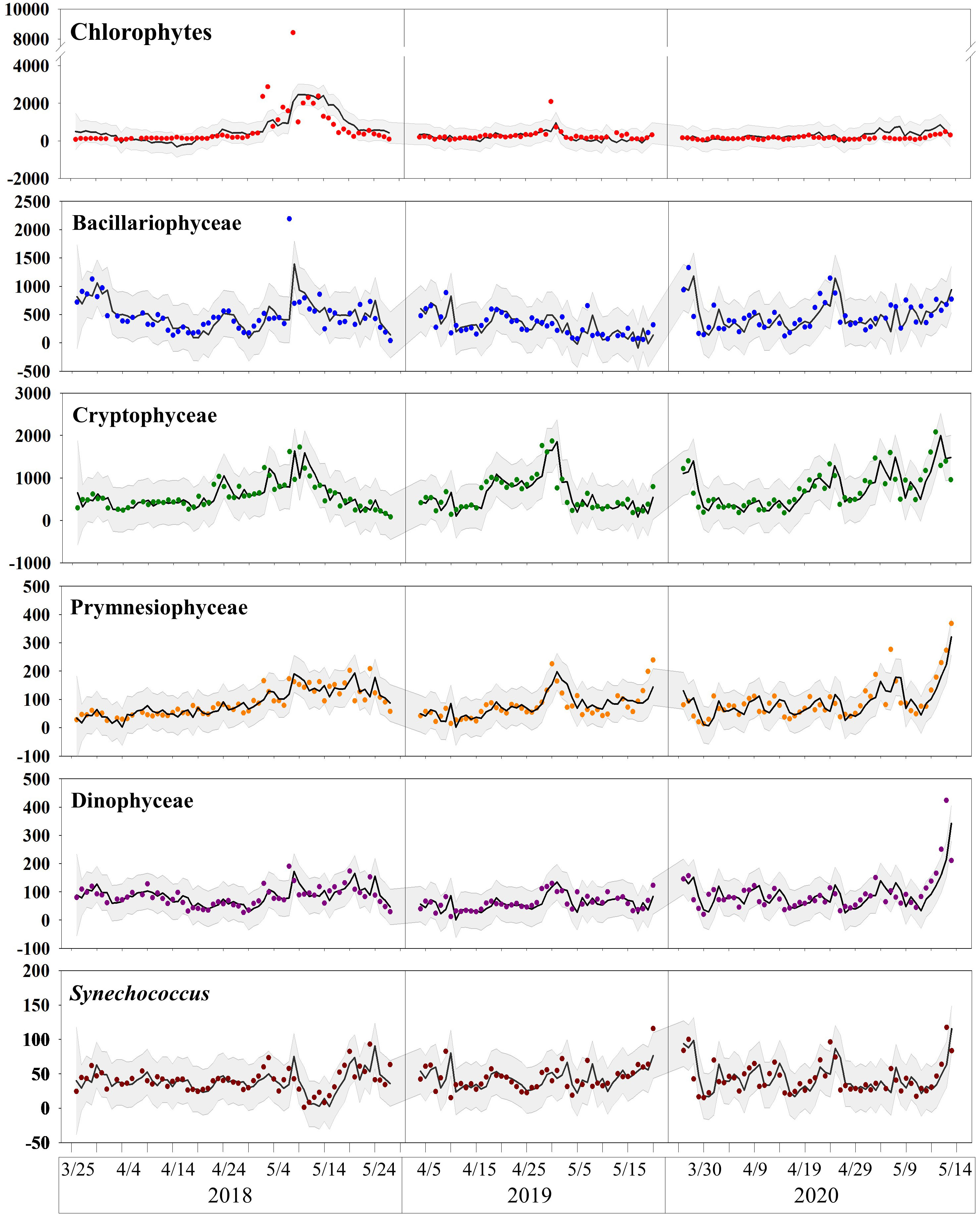
Figure 10 Comparison of actual and expected values obtained from the DFA model. Points represent actual values, line represents expected values, and gray shaded area indicates the 95% confidence interval of the model.

Plots used for model diagnostics are presented in Supplementary Figure S1. These plots confirm that there was no time-dependent pattern among the residuals and that the assumption of normal distribution was approximately met, although with some degree of tailing, indicating the failure of prediction for extreme values. No significant autocorrelation was detected among the residuals. These diagnostics demonstrate that the DFA model established here is valid, despite its failure to predict extreme values accurately.

Table 4 shows the coefficients obtained by the DFA model. The factor loadings for covariates show how environmental factors affect the biomass of each phytoplankton group. Each loading indicates the correlation between an environmental factor and the biomass of a group. Most phytoplankton groups have negative correlations with phosphate and nitrate concentrations. Overall, two groups appear in this analysis: one with larger negative factor loadings for phosphate and temperature, and one with smaller negative or positive loadings for phosphate and temperature. The first group includes chlorophytes, Bacillariophyceae, and Cryptophyceae, while the second group comprises Prymnesiophyceae, Dinophyceae, and Synechococcus.

TABLE 4

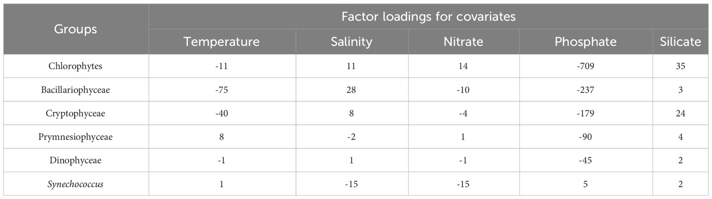
Table 4 Dynamic factor analysis (DFA) model results: factor loadings for covariates obtained from the DFA model.

Silicate had positive factor loadings for all groups. The loadings for Bacillariophyceae, Prymnesiophyceae, Dinophyceae, and Synechococcus ranged between 2 and 4, whereas chlorophytes and Cryptophyceae had high loadings of 35 and 24, respectively. Bacillariophyceae and Cryptophyceae have negative loadings for nitrate, similar to phosphate. Chlorophytes exhibit the largest positive loading.

4 Discussion

4.1 Applicability of time-series analysis based on data from fixed station S-ORS

DFA is a state-space model used for time-series analysis that fuses two multiple linear regressions, a covariate component and a state-space component. The covariate component explains the effects of environmental factors included in the model on phytoplankton biomass, whereas the state-space component captures the impacts of time-dependent environmental fluctuations that are not included as covariates in the model. These elements may be excluded from the model as a result of practical concerns such as ensuring model validity (e.g., to prevent excessive explanatory variables from undermining model robustness) or challenges associated with data collection. Unaccounted factors can range from the influence of zooplankton grazing and the physiological state of cells to atmospheric effects.

The factor loadings for the biomass of various phytoplankton groups, i.e., the covariate component, are shown in Table 4. These loadings are analogous to multiple linear regression slopes, and they provide substantial insights. For example, Bacillariophyceae had the lowest factor loading for temperature but the highest for salinity, which suggests a preference for unstable water columns that explains its dominance in early spring and persistence in waters beneath the pycnocline post-surface bloom. Although Cryptophyceae also had low factor loading for temperature and high factor loading for salinity, its values were less extreme than those of Bacillariophyceae. This difference may allow Cryptophyceae to contribute significantly to surface blooms in conditions where Bacillariophyceae struggles to survive. In contrast, Chlorophytes appear to thrive in relatively stable water columns. Their lowest factor loading for phosphate implies higher phosphate consumption, compared to other groups, and their positive factor loading for nitrate suggests that, although they consume nitrate, they consume it in lower amounts than phosphate. This finding suggests that chlorophyte surface blooms lead to surface phosphate limitation. The remaining three taxonomic groups appeared to favor more stable water columns and demonstrated higher resilience to low-phosphate environments, as inferred from their factor loadings.

A notable trend was observed in the state-space component of the DFA model: the state contribution ($\text{State loading}\times \text{State space}$; $\text{Γ}{\alpha }_t$) was significantly correlated with the group biomass of the previous day (chlorophytes: r = 0.68, Bacillariphyceae: r = 0.36, Cryptophyceae: r = 0.75, Prymnesiophyceae: r = 0.58, Dinophyceae: r = 0.72, Synechococcus: r = 0.54). This result indicates that, in addition to environmental impact, the biomass of the previous day contributes significantly to that of the following day.

Those patterns were not elucidated through network analysis. Bacillariophyceae, Dinophyceae, and Synechococcus had no edges connected with any environmental factors, which indicates that network analysis failed to explain the trend of the phytoplankton group along the environmental gradient. Thus, the network analysis was unable to reveal the combined effect of multiple variables, as it was based on single-correlation analysis. Network analysis has its strengths, although it failed to clarify the link between the environment and phytoplankton response in this study. Because our network analysis was conducted based on correlations between variables, it identified patterns that are typically difficult to discern through DFA and RDA due to multicollinearity. For example, network analysis revealed that stratification and density gradients in the pycnocline directly impacted the phytoplankton community, whereas the MLD showed no direct correlation. Moreover, our analysis also showed that wind and wave height have a much weaker impact on water stratification than temperature increases.

Although RDA is frequently utilized for analyzing phytoplankton communities, based on a combination of elements from multiple linear regression and PCA, its effectiveness can be compromised by data loss. Specifically, it often captures only overarching trends. In the RDA model employed in this study, the r² value was only 0.19, indicating significant data loss during the multiple linear regression phase. The subsequent PCA stage further accentuated this loss, with the RDA1 and RDA2 axes accounting for 46.89% and 32.32% of the variance, respectively, and representing an additional data loss of 20.79%. This oversimplification can be misinterpreted if the results are not carefully reviewed. For example, in the triplot, the pycnocline density gradient appeared to be positively correlated with the pycnocline depth and NP ratio, and to be negatively correlated with MLD; however, none of these inferences are true.

Therefore, it is clear that time-series data analysis can reveal detailed patterns that were not discerned through RDA or network analysis, which are primary analytical methods in community ecology. In this study, the time-series dataset was acquired at the fixed station S-ORS. As demonstrated in our research on the spring phytoplankton bloom pattern, S-ORS is a valuable facility for acquiring time-series datasets, and will contribute significantly to our understanding of oceanic processes.

4.2 Initiation of the surface phytoplankton bloom process

As shown in Table 3 and Figure 8, there were concurrent increases in phytoplankton biomass and parameters associated with weakened vertical mixing. However, in contrast to previous research suggesting that the formation of a shallow MLD above the critical depth initiates phytoplankton bloom in spring (Sverdrup, 1953; Rumyantseva et al., 2019), network analysis revealed that depth-associated parameters such as MLD and pycnocline depth did not directly affect the increase in phytoplankton biomass in early spring. Instead, parameters such as stratification and the density gradient in the pycnocline were more strongly correlated with Chl-a concentrations, relative to any other factors related to vertical mixing.

Weakened vertical mixing appears to result from an increase in SST, which is driven by increases in solar radiation and atmospheric temperature. Wind speed and wave height appear to have minimal impact on vertical mixing intensity or MLD, but they show weak correlations with pycnocline depth. Therefore, in the Yellow Sea, we concluded that the increase in biomass in spring results from weakened vertical mixing, which is caused by increased SST.

However, when Chl-a was divided into groups, the reactions to vertical mixing appeared to differ among groups. Chlorophytes, the dominant group within the surface bloom, appeared to be have direct interaction only with stratification, and Cryptophyceae, the second most dominant group in the surface bloom, exhibited complex interactions with stratification, atmosphere temperature, SST, density, pycnocline density gradient, and phosphate and silicates contents. As surface phytoplankton are associated with stratification, and most edges linked with Cryptophyceae are associated with vertical mixing, the surface phytoplankton bloom appears to have been initiated by the onset of vertical mixing. This finding is consistent with the concepts underlying the critical turbulence hypothesis (Huisman et al., 1999).

However, the biomass increase that occurred below the surface water before the surface bloom must be interpreted differently. Bacillariophyceae, the dominant group under the pycnocline, had no network edges connected with environmental factors. However, the RDA revealed strong preferences for a weak pycnocline density gradient and low temperature. This result is consistent with the DFA factor loadings on temperature and salinity. Therefore, we conclude that Bacillariophyceae prefers environmental conditions with active vertical mixing.

Although DFA analysis revealed that the increasing biomass of Bacillariophyceae was coupled with rapid nutrient consumption, we were unable to explain the faster consumption rate than that observed in the previous bloom, based on our data. However, the DFA state contribution showed a linear relationship with the biomass of the previous day, and Bacillairophyceae had the weakest correlation (r = 0.36). Thus, unlike other phytoplankton groups, the biomass of Bacillariophyceae was more substantially affected by the unknown variable than the biomass of the previous day or vertical mixing.

One strong possible explanation for this discrepancy is the disturbance and recovery hypothesis (Behrenfeld et al., 2013), which argues that in winter, phytoplankton–grazer interactions tend to become unbalanced as the relative water temperature increase alters the division and mortality rates of both phytoplankton and grazer. However, as our study did not collect data on grazers, this hypothesis cannot be tested using our data. However, interactions above and below surface blooms must occur based on different mechanisms, as different groups induce the bloom from each direction.

4.3 Phytoplankton spring bloom succession pattern observed repeatedly across years

The overall pattern of the spring bloom observed at S-ORS is illustrated in Figure 11. During the early spring season, the biomass of all phytoplankton groups is low, consisting mostly of Bacillariophyceae and Cryptophyceae. As temperature increases, the biomass of those taxa begins to increase, coinciding with decreasing concentrations of nutrients, especially phosphate, from the surface to bottom water.

FIGURE 11

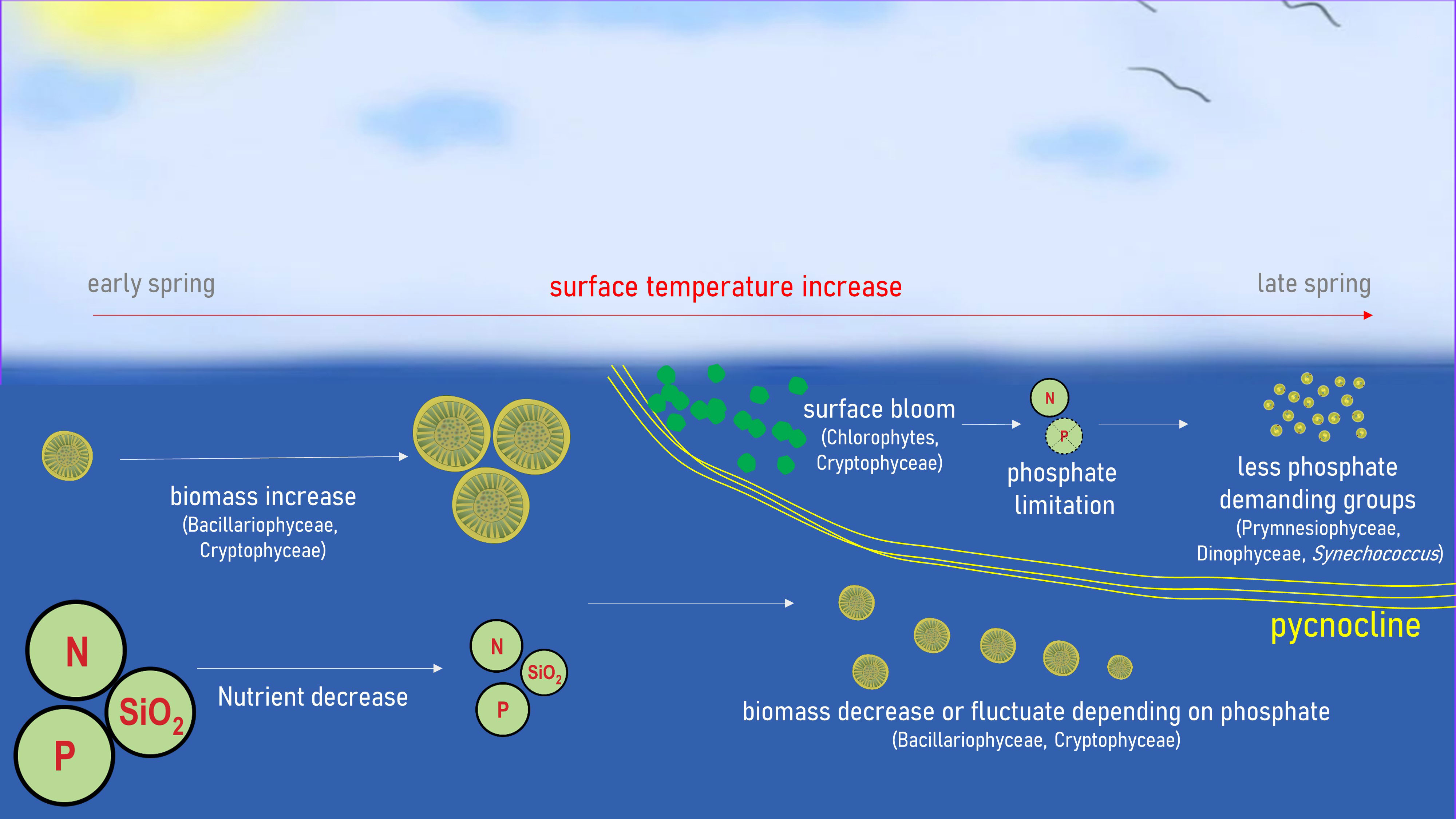
Figure 11 Schematic diagram of the spring bloom at S-ORS.

This pattern shifts when the surface temperature increases and the thermocline begins to develop in late April or early May. A rapid increase in chlorophyte biomass occurs during this period. The consistent timing of the chlorophyte bloom, along with the small negative factor loading for temperature, suggests that the stability of the water column may be an important contributor to the increase in chlorophyte biomass. Cryptophyceae also increase in biomass during this period, while Bacillariophyceae do not. The biomass of Bacillariophyceae above the pycnocline decreases during this period, while their biomass below the pycnocline either decreases or fluctuates both during and after this period. This pattern is caused by the preference of the Bacillariophyceae for a turbulent water column over a stable water column, as shown by DFA and RDA. The availability of phosphate appears to be a critical determinant of Bacillariophyceae biomass.

As the DFA model indicates, chlorophytes have the highest consumption rate of phosphate, but not as much nitrate. The chlorophyte bloom above the pycnocline leads to depletion of phosphate, resulting in extremely high N:P ratio values. This stress, stemming from phosphate limitation as evidenced by the extreme N:P ratio, leads to a subsequent decrease in the biomass of nutrient-demanding groups such as chlorophytes, Bacillariophyceae, and Cryptophyceae (Egge, 1998; Lafarga-De la Cruz et al., 2006; Lin et al., 2016; Ramos-Rodriíguez et al., 2017; Tragin and Vaulot, 2018; Andersen et al., 2020). While their preference for phosphate over nitrate might vary based on environmental and physiological states, given the clear phosphate limitation in the surface water, it’s reasonable to infer that this limitation restricts their biomass. This trend is coupled with a slight increase in Prymnesiophyceae and Synechococcus, which have lower nutrient demand. The Dinophyceae, known to be nutrient-demanding, also increase their biomass in this period. Lin et al. (2016) summarized the factors contributing to the rise of Dinophyceae in nutrient-limited late spring: their motility allows them to migrate vertically (Sinclair and Kamykowski, 2008; Hall and Paerl, 2011), accessing deeper nutrient-rich waters; their ability to utilize DOP and DON (Sunda et al., 2006; Burkholder et al., 2008); their capacity for phagotrophy; and their defense mechanisms that deter grazing (Sunda et al., 2006; Hong et al., 2012; Waggett et al., 2012; Hardison et al., 2013).

In 2019, the phosphate concentration was the lowest compared to the other two years. Consequently, the nitrate concentration did not decrease as significantly as it did in the other years. This is likely because phosphate limitation hindered the utilization of nitrate by phytoplankton. As phosphate limitated the surface chlorophyte peak appears to be smaller in 2019 than 2018. Furthermore, the surface increases of Prymnesiophyceae, Dinophyceae, and Synechococcus immediately after the chlorophyte peak appears to be less significant and somewhat delayed compared to 2018. These patterns indicate that concentrations of nutrients (e.g., phosphate) and temperature are the major factors that determine phytoplankton community composition, consistent with multiple recent studies (Skákala and Lazzari, 2021; Hyun et al., 2023; Zhang G. et al., 2023).

Overall, the concentration of phosphate appears to be the most significant determinant of the magnitude and timing of the spring bloom. The increase in temperature, which results in the formation of a pycnocline and induces the chlorophyte bloom, is another important factor during this period. However, in 2020, the temperature increase in surface water was further delayed, resulting in a distinct pattern.

4.4 Differences in spring bloom patterns among 3 years and their environmental drivers

While the difference between 2018 and 2019 is generally limited to phosphate concentration, 2020 exhibited significantly different physical characteristics, leading to a different spring bloom pattern. The formation of a pycnocline, which initially induces a chlorophyte bloom above it that later switches to less phosphate-demanding groups, was significantly delayed (until mid- to late May) in 2020. As a result, no chlorophyte bloom occurred, which prevented phosphate limitation. This absence of phosphate limitation allowed for a longer period of high Bacillariophyceae and Cryptophyceae biomass throughout the water column compared to the previous 2 years. As the pycnocline began to develop in mid-May, the biomass of all phytoplankton groups increased simultaneously, but the maximum chlorophyll concentration in surface water was much lower than in the other 2 years.

Overall, a phytoplankton spring bloom anomaly occurred in 2020 due to weakened stratification (Kim et al., 2023a). According to a previous studies, this weakened thermal stratification was primarily induced by latent heat flux release driven by strong northwesterly winds in April 2020, accompanied by anticyclonic and cyclonic circulation patterns over Siberia and the East Sea (Kim et al., 2022; Kim et al., 2023b). The anomaly was also influenced by warm winter temperatures. The prevailing northwesterly winds generated a cold surface anomaly, which increased vertical water column mixing, resulting in a weakened phytoplankton spring bloom. These factors combined to create conditions that were not conducive to a healthy spring bloom in the Yellow Sea.

Climate change may have played a role in the weakened stratification observed in the Yellow Sea in 2020. Climate change can affect ocean temperature, currents, and atmospheric conditions, all of which can impact ocean stratification patterns. Further research is needed to clarify the complex interactions among these factors and their potential impacts on marine ecosystems. In the era of big data in marine science, characterized by an explosion of in situ observations, quantitative remote sensing products, techniques for managing uncertainties in marine remote sensing data, and efforts to connect historical and modern datasets are particularly important for accurate monitoring of the spatial and temporal distributions and variabilities of phytoplankton community composition (Mélin, 2019; Brewin et al., 2023; Zhang Y. et al., 2023).

5 Conclusions

This study elucidated the intricate dynamics of the seasonal phytoplankton bloom in the Yellow Sea. We found that the initiation of the phytoplankton spring bloom process is closely associated with weakened vertical mixing, which is driven by increased SST. Our research revealed a consistent pattern of phytoplankton spring bloom succession across years; changes in phosphate concentration and temperature played significant roles. However, the year 2020 exhibited a unique pattern due to delayed pycnocline formation and weakened stratification, highlighting the potential impacts of climate change on this process. These findings underscore the complex interplay between physical and biological factors in terms of shaping phytoplankton dynamics; they suggest that further research is needed to clarify these interactions and potential impacts on marine ecosystems.

Taxonomically, chlorophytes and Cryptophyceae, which dominated the surface bloom, interacted directly with stratification. Bacillariophyceae, which was dominant beneath the pycnocline, appeared to prefer turbulent water conditions. As the surface water became nutrient-limited, there was a shift to late successional groups such as Dinophyceae, Prymnesiophyceae, and Synechococcus.

Data availability statement

The raw data supporting the conclusions of this article will be made available by the authors, without undue reservation.

Author contributions

JN and MH conceptualized and designed the study. MH, JN, and KR developed the methodology. MH, DC, HL, JL, and JW conducted data curation. MH managed the software. MH and G-UK performed the formal analysis. MH, KR, HL, JW, WY, JL, and JJ conducted the investigation. JN, J-YJ, and DC provided resources. MH, G-UK, and KR curated the data. MH, WY, HL, JW, and JN wrote the first draft of the manuscript. JN, YL, J-YJ, DC, KR, G-UK, JL, JJ, and CL wrote, reviewed, and edited the manuscript. MH and JN created the visualizations. JN, DC, and YL supervised the project. JN and J-YJ administered the project and acquired the funding. All authors contributed to the article and approved the submitted version.

Funding

The authors declare financial support was received for the research, authorship, and/or publication of this article. This research was supported by Korea Institute of Marine Science & Technology Promotion(KIMST) funded by the Ministry of Oceans and Fisheries (grant nos. 20210607 and 20210696).

Acknowledgments

We thank the Korea Hydrographic and Oceanographic Agency for their assistance with our stay at S-ORS and for providing sensor data acquired at the facility.

Conflict of interest

The authors declare that the research was conducted in the absence of any commercial or financial relationships that could be construed as a potential conflict of interest.

Publisher’s note

All claims expressed in this article are solely those of the authors and do not necessarily represent those of their affiliated organizations, or those of the publisher, the editors and the reviewers. Any product that may be evaluated in this article, or claim that may be made by its manufacturer, is not guaranteed or endorsed by the publisher.

Supplementary material

The Supplementary Material for this article can be found online at: https://www.frontiersin.org/articles/10.3389/fmars.2023.1280612/full#supplementary-material

References

Andersen I. M., Williamson T. J., González M. J., Vanni M. J. (2020). Nitrate, ammonium, and phosphorus drive seasonal nutrient limitation of chlorophytes, cyanobacteria, and diatoms in a hyper-eutrophic reservoir. Limnology Oceanography 65 (5), 962–978. doi: 10.1002/lno.11363

CrossRef Full Text | Google Scholar

Barton A. D., Pershing A. J., Litchman E., Record N. R., Edwards K. F., Finkel Z. V., et al. (2013). The biogeography of marine plankton traits. Ecol. Lett. 16 (4), 522–534. doi: 10.1111/ele.12063

PubMed Abstract | CrossRef Full Text | Google Scholar

Basu S., Mackey K. R. (2018). Phytoplankton as key mediators of the biological carbon pump: Their responses to a changing climate. Sustainability 10 (3), 869. doi: 10.3390/su10030869

CrossRef Full Text | Google Scholar

Behrenfeld M. J., Doney S. C., Lima I., Boss E. S., Siegel D. A. (2013). Annual cycles of ecological disturbance and recovery underlying the subarctic Atlantic spring plankton bloom. Global biogeochemical cycles 27 (2), 526–540. doi: 10.1002/gbc.20050

CrossRef Full Text | Google Scholar

Bidigare R. R., Buttler F. R., Christensen S. J., Barone B., Karl D. M., Wilson S. T. (2014). Evaluation of the utility of xanthophyll cycle pigment dynamics for assessing upper ocean mixing processes at Station ALOHA. J. plankton Res. 36 (6), 1423–1433. doi: 10.1093/plankt/fbu069

CrossRef Full Text | Google Scholar

Brewin R. J., Pitarch J., Dall’Olmo G., van der Woerd H. J., Lin J., Sun X., et al. (2023). Evaluating historic and modern optical techniques for monitoring phytoplankton biomass in the Atlantic Ocean. Front. Mar. Sci. 10, 1111416. doi: 10.3389/fmars.2023.1111416

CrossRef Full Text | Google Scholar

Burkholder J. M., Glibert P. M., Skelton H. M. (2008). Mixotrophy, a major mode of nutrition for harmful algal species in eutrophic waters. Harmful algae 8 (1), 77–93. doi: 10.1016/j.hal.2008.08.010

CrossRef Full Text | Google Scholar

Choi D. H., An S. M., Chun S., Yang E. C., Selph K. E., Lee C. M., et al. (2016). Dynamic changes in the composition of photosynthetic picoeukaryotes in the northwestern Pacific Ocean revealed by high-throughput tag sequencing of plastid 16S rRNA genes. FEMS Microbiol. Ecol. 92 (2):fiv170. doi: 10.1093/femsec/fiv170

CrossRef Full Text | Google Scholar

de Boyer Montégut C., Madec G., Fischer A. S., Lazar A., Iudicone D. (2004). Mixed layer depth over the global ocean: An examination of profile data and a profile-based climatology. J. Geophysical Research: Oceans 109 (C12003). doi: 10.1029/2004JC002378

CrossRef Full Text | Google Scholar

Egge J. (1998). Are diatoms poor competitors at low phosphate concentrations? J. Mar. Syst. 16 (3-4), 191–198. doi: 10.1016/S0924-7963(97)00113-9

CrossRef Full Text | Google Scholar

Eggers S. L., Lewandowska A. M., Barcelos e Ramos J., Blanco-Ameijeiras S., Gallo F., Matthiessen B. (2014). Community composition has greater impact on the functioning of marine phytoplankton communities than ocean acidification. Global Change Biol. 20 (3), 713–723. doi: 10.1111/gcb.12421

CrossRef Full Text | Google Scholar

Hall N. S., Paerl H. W. (2011). Vertical migration patterns of phytoflagellates in relation to light and nutrient availability in a shallow microtidal estuary. Mar. Ecol. Prog. Ser. 425, 1–19. doi: 10.3354/meps09031

CrossRef Full Text | Google Scholar

Hardison D. R., Sunda W. G., Shea D., Litaker R. W. (2013). Increased toxicity of Karenia brevis during phosphate limited growth: ecological and evolutionary implications. PloS One 8 (3), e58545. doi: 10.1371/journal.pone.0058545

PubMed Abstract | CrossRef Full Text | Google Scholar

Harris G. (2012). Phytoplankton ecology: structure, function and fluctuation (Amsterdam, Netherlands: Springer Science & Business Media).

Google Scholar

Hashioka T., Vogt M., Yamanaka Y., Le Quéré C., Buitenhuis E., Aita M. N., et al. (2013). Phytoplankton competition during the spring bloom in four plankton functional type models. Biogeosciences 10 (11), 6833–6850. doi: 10.5194/bg-10-6833-2013

CrossRef Full Text | Google Scholar

Hilligsøe K. M., Richardson K., Bendtsen J., Sørensen L.-L., Nielsen T. G., Lyngsgaard M. M. (2011). Linking phytoplankton community size composition with temperature, plankton food web structure and sea–air CO2 flux. Deep Sea Res. Part I: Oceanographic Res. Papers 58 (8), 826–838. doi: 10.1016/j.dsr.2011.06.004

CrossRef Full Text | Google Scholar

Holmes E. E., Scheuerell M. D., Ward E. J. (2021a) Analysis of multivariate time-series using the MARSS package (version 3.11.4) [R package]. Available at: https://CRAN.R-project.org/package=MARSS/vignettes/UserGuide.pdf.

Google Scholar

Holmes E. E., Ward E. J., Kellie W. (2012). MARSS: multivariate autoregressive state-space models for analyzing time-series data. R J. 4 (1), 11. doi: 10.32614/RJ-2012-002

CrossRef Full Text | Google Scholar

Holmes E. E., Ward E. J., Scheuerell M. D., Wills K. (2021b) MARSS: Multivariate Autoregressive State-Space Modeling. (version 3.11.4) [R package]. Available at: https://CRAN.R-project.org/package=MARSS.

Google Scholar

Hong J., Talapatra S., Katz J., Tester P. A., Waggett R. J., Place A. R. (2012). Algal toxins alter copepod feeding behavior. PloS One 7 (5), e36845. doi: 10.1371/journal.pone.0036845

PubMed Abstract | CrossRef Full Text | Google Scholar

Huisman J., van Oostveen P., Weissing F. J. (1999). Critical depth and critical turbulence: two different mechanisms for the development of phytoplankton blooms. Limnology oceanography 44 (7), 1781–1787. doi: 10.4319/lo.1999.44.7.1781

CrossRef Full Text | Google Scholar

Hyun S., Cape M. R., Ribalet F., Bien J. (2023). Modeling cell populations measured by flow cytometry with covariates using sparse mixture of regressions. Ann. Appl. Stat 17 (1), 357. doi: 10.1214/22-AOAS1631

PubMed Abstract | CrossRef Full Text | Google Scholar

Hyun M. J., Won J., Choi D. H., Lee H., Lee Y., Lee C. M., et al. (2022). A CHEMTAX study based on picoeukaryotic phytoplankton pigments and next-generation sequencing data from the ulleungdo–dokdo marine system of the east sea (Japan sea): improvement of long-unresolved underdetermined bias. J. Mar. Sci. Eng. 10 (12), 1967. doi: 10.3390/jmse10121967

CrossRef Full Text | Google Scholar

Karl D. M., Björkman K. M., Dore J. E., Fujieki L., Hebel D. V., Houlihan T., et al. (2001). Ecological nitrogen-to-phosphorus stoichiometry at station ALOHA. Deep Sea Res. Part II: Topical Stud. Oceanography 48 (8-9), 1529–1566. doi: 10.1016/S0967-0645(00)00152-1

CrossRef Full Text | Google Scholar

Karl D. M., Church M. J. (2017). Ecosystem structure and dynamics in the North Pacific Subtropical Gyre: new views of an old ocean. Ecosystems 20, 433–457. doi: 10.1007/s10021-017-0117-0

CrossRef Full Text | Google Scholar

Karl D. M., Church M. J. (2019). Station ALOHA: A gathering place for discovery, education, and scientific collaboration: station ALOHA: A gathering place for discovery, education, and scientific collaboration. Limnology Oceanography Bull. 28 (1), 10–12. doi: 10.1002/lob.10285

CrossRef Full Text | Google Scholar

Kim Y. S., Jang C. J., Noh J. H., Kim K.-T., Kwon J.-I., Min Y., et al. (2019). A Yellow Sea monitoring platform and its scientific applications. Front. Mar. Sci. 6, 601. doi: 10.3389/fmars.2019.00601

CrossRef Full Text | Google Scholar

Kim G.-U., Lee J., Kim Y. S., Noh J. H., Kwon Y. S., Lee H., et al. (2023a). Impact of vertical stratification on the 2020 spring bloom in the Yellow Sea. Sci. Rep 13 (1), 14320. doi: 10.1038/s41598-023-40503-z

PubMed Abstract | CrossRef Full Text | Google Scholar

Kim G.-U., Lee K., Lee J., Jeong J.-Y., Lee M., Jang C. J., et al. (2022). Record-breaking slow temperature evolution of spring water during 2020 and its impacts on spring bloom in the Yellow Sea. Front. Mar. Sci. 562. doi: 10.3389/fmars.2022.824361

CrossRef Full Text | Google Scholar

Kim G.-U., Oh H., Kim Y. S., Son J.-H., Jeong J.-Y. (2023b). Causes for an extreme cold condition over Northeast Asia during April 2020. Sci. Rep. 13 (1), 3315. doi: 10.1038/s41598-023-29934-w

PubMed Abstract | CrossRef Full Text | Google Scholar

Lafarga-De la Cruz F., Valenzuela-Espinoza E., Millán-Núnez R., Trees C. C., Santamaría-del-Ángel E., Núnez-Cebrero F. (2006). Nutrient uptake, chlorophyll a and carbon fixation by Rhodomonas sp.(Cryptophyceae) cultured at different irradiance and nutrient concentrations. Aquacultural Eng. 35 (1), 51–60. doi: 10.1016/j.aquaeng.2005.08.004

CrossRef Full Text | Google Scholar

Latasa M. (2007). Improving estimations of phytoplankton class abundances using CHEMTAX. Mar. Ecol. Prog. Ser. 329, 13–21. doi: 10.3354/meps329013

CrossRef Full Text | Google Scholar

Lin S., Litaker R. W., Sunda W. G. (2016). Phosphorus physiological ecology and molecular mechanisms in marine phytoplankton. J. Phycology 52 (1), 10–36. doi: 10.1111/jpy.12365

CrossRef Full Text | Google Scholar

Litchman E., de Tezanos Pinto P., Edwards K. F., Klausmeier C. A., Kremer C. T., Thomas M. K. (2015). Global biogeochemical impacts of phytoplankton: a trait-based perspective. J. Ecol. 103 (6), 1384–1396. doi: 10.1111/1365-2745.12438

CrossRef Full Text | Google Scholar

Mackey M., Mackey D., Higgins H., Wright S. (1996). CHEMTAX-a program for estimating class abundances from chemical markers: application to HPLC measurements of phytoplankton. Mar. Ecol. Prog. Ser. 144, 265–283. doi: 10.3354/meps144265

CrossRef Full Text | Google Scholar

Mélin F. (2019). Uncertainties in ocean colour remote sensing. International Ocean Colour Coordinating Group (IOCCG): Dartmouth, NS, Canada

Google Scholar

Nissen C., Gruber N., Münnich M., Vogt M. (2021). Southern Ocean phytoplankton community structure as a gatekeeper for global nutrient biogeochemistry. Global Biogeochemical Cycles 35 (8), e2021GB006991. doi: 10.1029/2021GB006991

CrossRef Full Text | Google Scholar

Olita A., Sparnocchia S., Cusí S., Fazioli L., Sorgente R., Tintoré J., et al. (2014). Observations of a phytoplankton spring bloom onset triggered by a density front in NW Mediterranean. Ocean Sci. 10 (4), 657–666. doi: 10.5194/os-10-657-2014

CrossRef Full Text | Google Scholar

Ramos-Rodríguez E., Perez-Martinez C., Conde-Porcuna J. M. (2017). Strict stoichiometric homeostasis of Cryptomonas pyrenoidifera (Cryptophyceae) in relation to N: P supply ratios. J. Limnol 76 (1), 182–189. doi: 10.4081/jlimnol.2016.1487

CrossRef Full Text | Google Scholar

R Core Team (2022). “R: A language and environment for statistical computing” (Vienna, Austria: Foundation for Statistical Computing).

Google Scholar

Roy S., Llewellyn C. A., Egeland E. S., Johnsen G. (2011). Phytoplankton pigments: characterization, chemotaxonomy and applications in oceanography. (Cambridge, UK: Cambridge University Press).

Google Scholar

Rumyantseva A., Henson S., Martin A., Thompson A. F., Damerell G. M., Kaiser J., et al. (2019). Phytoplankton spring bloom initiation: The impact of atmospheric forcing and light in the temperate North Atlantic Ocean. Prog. oceanography 178, 102202. doi: 10.1016/j.pocean.2019.102202

CrossRef Full Text | Google Scholar

Schlitzer R. (2022). “Ocean data view (software)”. Bremerhaven, Germany: Alfred Wegener Institue

Google Scholar

Simpson G. L., Blanchet F. G., Kindt R., Legendre P., Minchin P. R., O’Hara R. B., et al. (2022) vegan: Community Ecology Package (version 2.6-2) [R package]. Available at: https://CRAN.R-project.org/package=vegan.

Google Scholar

Sinclair G. A., Kamykowski D. (2008). Benthic–pelagic coupling in sediment-associated populations of Karenia brevis. J. plankton Res. 30 (7), 829–838. doi: 10.1093/plankt/fbn042

CrossRef Full Text | Google Scholar

Skákala J., Lazzari P. (2021). Low complexity model to study scale dependence of phytoplankton dynamics in the tropical Pacific. Phys. Rev. E 103 (1), 012401. doi: 10.1103/PhysRevE.103.012401

PubMed Abstract | CrossRef Full Text | Google Scholar

Sommer U., Adrian R., De Senerpont Domis L., Elser J. J., Gaedke U., Ibelings B., et al. (2012). Beyond the Plankton Ecology Group (PEG) model: mechanisms driving plankton succession. Annu. Rev. ecology evolution systematics 43, 429–448. doi: 10.1146/annurev-ecolsys-110411-160251

CrossRef Full Text | Google Scholar

Sunda W. G., Graneli E., Gobler C. J. (2006). Positive feedback and the development and persistence of ecosystem disruptive algal blooms 1. J. Phycology 42 (5), 963–974. doi: 10.1111/j.1529-8817.2006.00261.x

CrossRef Full Text | Google Scholar

Sverdrup H. (1953). On conditions for the vernal blooming of phytoplankton. J. Cons. Int. Explor. Mer 18 (3), 287–295. doi: 10.1093/icesjms/18.3.287

CrossRef Full Text | Google Scholar

Tragin M., Vaulot D. (2018). Green microalgae in marine coastal waters: The Ocean Sampling Day (OSD) dataset. Sci. Rep. 8 (1), 14020. doi: 10.1038/s41598-018-32338-w

PubMed Abstract | CrossRef Full Text | Google Scholar

Van den Engh G. J., Doggett J. K., Thompson A. W., Doblin M. A., Gimpel C. N., Karl D. M. (2017). Dynamics of Prochlorococcus and Synechococcus at station ALOHA revealed through flow cytometry and high-resolution vertical sampling. Front. Mar. Sci. 4, 359. doi: 10.3389/fmars.2017.00359

CrossRef Full Text | Google Scholar

Van den Meersche K., Soetaert K. (2022) Package ‘BCE’ (version 2.2.0) [R package]. Available at: https://CRAN.R-project.org/package=BCE.

Google Scholar

Van den Meersche K., Soetaert K., Middelburg J. J. (2008). A Bayesian compositional estimator for microbial taxonomy based on biomarkers. Limnology Oceanography-Methods 6, 190–199. doi: 10.4319/lom.2008.6.190

CrossRef Full Text | Google Scholar

Waggett R. J., Hardison D. R., Tester P. A. (2012). Toxicity and nutritional inadequacy of Karenia brevis: synergistic mechanisms disrupt top-down grazer control. Mar. Ecol. Prog. Ser. 444, 15–30. doi: 10.3354/meps09401

CrossRef Full Text | Google Scholar

Weithoff G., Beisner B. E. (2019). Measures and approaches in trait-based phytoplankton community ecology–from freshwater to marine ecosystems. Front. Mar. Sci. 6, 40. doi: 10.3389/fmars.2019.00040

CrossRef Full Text | Google Scholar

Wickham H. (2016). ggplot2: elegant graphics for data analysis (Springer-Verlag New York, USA).

Google Scholar

Winder M., Sommer U. (2012). Phytoplankton response to a changing climate. Hydrobiologia 698, 5–16. doi: 10.1007/s10750-012-1149-2

CrossRef Full Text | Google Scholar

Worden A. Z., Follows M. J., Giovannoni S. J., Wilken S., Zimmerman A. E., Keeling P. J. (2015). Rethinking the marine carbon cycle: factoring in the multifarious lifestyles of microbes. Science 347 (6223), 1257594. doi: 10.1126/science.1257594

PubMed Abstract | CrossRef Full Text | Google Scholar

Yang W., Noh J. H., Lee H., Lee Y., Choi D. H. (2021). Weekly variation of prokaryotic growth and diversity in the inner bay of Yeong-do, Busan. Ocean Polar Res. 43 (1), 31–43. doi: 10.4217/OPR.2021.43.1.031

CrossRef Full Text | Google Scholar

Zapata M., Rodríguez F., Garrido J. L. (2000). Separation of chlorophylls and carotenoids from marine phytoplankton: a new HPLC method using a reversed phase C8 column and pyridine-containing mobile phases. Mar. Ecol. Prog. Ser. 195, 29–45. doi: 10.3354/meps195029

CrossRef Full Text | Google Scholar

Zhang G., Liu Z., Zhang Z., Ding C., Sun J. (2023). The impact of environmental factors on the phytoplankton communities in the Western Pacific Ocean: HPLC-CHEMTAX approach. Front. Mar. Sci. 10, 1185939. doi: 10.3389/fmars.2023.1185939

CrossRef Full Text | Google Scholar

Zhang Y., Shen F., Sun X., Tan K. (2023). Marine big data-driven ensemble learning for estimating global phytoplankton group composition over two decades, (1997–2020). Remote Sens. Environ. 294, 113596. doi: 10.1016/j.rse.2023.113596

CrossRef Full Text | Google Scholar