Anomaly detection in feature space for detecting changes in phytoplankton populations

1 Introduction

The term plankton refers to drifter microorganisms that flow passively in the water. It includes unicellular plants that contain chlorophyll and perform photosynthesis (Winder and Sommer, 2012), named Phytoplankton, and generally millimetric or smaller animals, called Zooplankton (Brierley, 2017). Phytoplankton significantly impacts global climate regulation and has produced around 50% of the total oxygen in the atmosphere (Benfield et al., 2007). Moreover, it is responsible for approximately 45% of global earth primary production (Uitz et al., 2010), with plankton diatoms being responsible for fixing at least a quarter of the inorganic carbon in the ocean on an annual basis (Brierley, 2017). Zooplankton pastures on Phytoplankton, and is predated by fish and other aquatic animals, collocating these fundamental organisms at the core of the aquatic food chain. Importantly, Plankton organisms can be regarded as a good indicator of climate change and modifications (Hays et al., 2005) with high sensitivity, as subtle environmental perturbations can be magnified by the responses of biological communities (Taylor et al., 2002). Plankton microorganisms, in fact, may exhibit distinct physiological modifications as a response to even slight perturbations in the aquatic environment, resulting in changes at an individual and population level. At an individual level, such physiological alterations may correspond to morphological and behavioral changes. To provide an example, when encountering chemicals released by predators, numerous zooplankton physiologically exhibit morphological and behavioral responses (Ohman, 1988). On a population level, environmental changes may affect biodiversity and species abundance, possibly reverting species dominance (Hanazato, 2001). Recently, it has been proposed to employ plankton as biosensors exploiting acquired images and machine learning tools (Pastore et al., 2019; Pastore et al., 2022). This involves establishing a baseline for the average plankton morphology of known classes, included in an initial training set, and using it to identify deviations, which could serve as indicators of environmental changes, whether of human origin or natural.

In the last years, a massive amount of plankton images has been gathered, thanks to technologically advanced automatic acquisition systems (Benfield et al., 2007; Lombard et al., 2019). The availability of such an increasingly large number of images makes manual species identification and image analysis impractical (Alfano et al,. 2022), paving the way to machine learning-based solutions. The majority of available works on automatic plankton image classification involve supervised learning methods relying on annotations. Hand-crafted descriptors based on shape, texture, or multiscale visual features can be used alongside a trainable classifier: for example in Sosik and Olson (2007), multiple hand-crafted features are computed from raw images and then fed to an SVM classifier, while in Zheng et al. (2017) feature selection is employed on several sets of hand-crafted features to maximize features importance, and multiple kernel learning (Gönen and Alpaydın, 2011) is adopted by the authors and provides improved classification performances on different plankton image datasets, with respect to comparable approaches. With the development and diffusion of deep neural networks for vision tasks, deep learning-driven solutions have increasingly been adopted for plankton image classification: in the last few years, the best-performing techniques have been based on ensembles composed of many deep networks, capable of yielding quasi-optimal classification performance on annotated datasets of varying size (Lumini and Nanni, 2019; Kyathanahally et al., 2021; Maracani et al., 2023). Recent works related to plankton image analysis and classification experimented with hybrid approaches, such as Semi-Supervised Learning applied to population counting in Orenstein et al. (2020a), or classification through Content-Based Image Retrieval (Yang et al., 2022). We can also find two works employing anomaly detection and outlier-exposure techniques to aid classifiers in taxonomic classification: in Pu et al. (2021) the authors build a dataset of anomalies and a custom loss to both improve classification performances and to detect anomalous images; Walker and Orenstein (2021) employ Hard-Negative-Mining and Background Resampling to improve the detection rate of rare classes. Additionally, for the purpose of this work, it is worth pointing out that in Orenstein and Beijbom (2017) it is shown that pre-training deep neural networks on large-scale general-purpose image datasets gives a better transfer-learning baseline for plankton image classification over the one that could be obtained by pre-training on in-domain planktonic image datasets, even if of comparable size (Maracani et al., 2023). An image-based machine learning framework for the usage of plankton as a biosensor has been proposed in Pastore et al, 2019; Pastore et al, 2022). In Pastore et al. (2019) the authors extract a set of 128 descriptors from a subset of plankton images with 100 images for 10 classes, extracted from the WHOI dataset. The engineered descriptors incorporate both shape-based features, including geometric descriptors and image moments, and texture-based features, such as Haralick and local binary patterns. The authors employ a one-class SVM anomaly detection algorithm, proposing to detect deviation from the average appearance for each of the training classes, as an indicator of potential environmental perturbations. In Pastore et al. (2022), a custom anomaly detection algorithm, TailDeTect (TDT) is exploited to perform novel class detection, starting from an available annotated set of plankton images. The authors exploit a set of 131 hand-crafted features, reaching a high accuracy in the novel class detection task, for an in-house plankton dataset, acquired using a lensless microscope and released in Pastore et al. (2020). An important limitation of these works is the coarse granularity of the investigated plankton dataset. A fundamental prerequisite for a machine learning framework to be actually used in the task of suggesting potential environmental changes using plankton images is represented by the possibility of correctly separating morphologically fine-grained classes, where the intra-class morphological features are in the same order of magnitude as the inter-class ones. Moreover, recent works on unsupervised learning of plankton images (Alfano et al,. 2022), have shown that features extracted by means of ImageNet pre-trained deep neural networks provide an embedding leading to higher accuracy than hand-crafted features.

In this context, we propose a semi-automatic approach where a machine learning framework is designed to automatically detect anomalies in the feature space extracted from acquired phytoplankton images, while an engineering pipeline is sketched to exploit plankton’s feedback for revealing potential environmental changes. Our machine learning framework consists in anomaly detection algorithms coupled to features extracted from acquired images by means of ImageNet pre-trained Vision Transformers, relying on the possibility of detecting samples belonging to classes with shape or morphology significantly different with respect to the training ones. Such anomalies can be related to different main sources, including (i) Morphological modifications potentially linked to environmental changes human-made or natural; (ii) novel classes (i.e., classes not included in the training set); (iii) image artifacts (caused by different factors, including the acquisition system and water condition). Besides, it is known that distribution shifts for the same species across time are likely to happen (González et al., 2017). Thus, we may expect a certain number of anomalies to be detected on a regular basis at the site of acquisition. We envision determining critical situations corresponding to a significant increase in the detected anomalies with respect to the average number of anomalies per time. At this stage, we propose to have a human in the loop, so that a selection of such anomalies may be provided to experts in the field to actually discriminate between the different sources of anomalies, potentially recognizing environmental threats. To summarize, the main contributions of this paper can be regarded as follows: (i) We introduce an anomaly detection-based approach for detecting significant variations in acquired phytoplankton images, potentially linked to environmental changes. Differently from the state-of-the-art, we exploit a set of features extracted by an ImageNet22K pre-trained vision transformer, coupled to a dimensionality reduction algorithm based on PCA. Assuming the availability of an initial annotated dataset, we propose to train one anomaly detector for each of the available classes, further arranging them in a parallel architecture, capable of detecting in-class samples and global anomalies, that is, a sample that is simultaneously rejected by all the trained anomaly detectors. The designed approach is modular, allowing to add new classes by training a new corresponding anomaly detector, without the need to re-train the other detectors. We test the proposed approach on two fine-grained publicly available plankton datasets (WHOI22 (Sosik and Olson, 2007) and WHOI40 (Pastore et al., 2020), containing grayscale microscopic images of phytoplankton collected with the Imaging FlowCytobot (IFCB) system typically used as benchmarks for plankton image classification (Zheng et al. (2017); Lumini et al., 2020; Kyathanahally et al., 2021). (ii) We build a phytoplankton image dataset that we name WHOI15, considering 15 classes including detritus among 4 different years of acquisition (from 2007 to 2010), proving that our anomaly detection algorithms can generalize well in recognizing anomalies or a novel class in different years of acquisition with respect to the training one. Exploiting the concept of global anomalies, we sketch an engineering pipeline capable of providing alerts representing phytoplankton changes potentially related to environmental perturbations.

The remainder of the paper is organized as follows: in Sec. 2, we describe the proposed approach and its main components. In Sec. 3, we describe the datasets used in this work, providing experiment details and results, later discussed in Sec. 4.

2 Methods

In this study, we introduce a novel approach for automatically determining anomalies in phytoplankton images, that can be further related to environmental changes. The designed method, as depicted in Figure 1, consists of three key stages: (i) Feature extraction and compression, (ii) Anomaly detection, and (iii) Anomaly storage and analysis. Initially, we assume the availability of a plankton image dataset with expert-provided labels. These images are then processed using an ImageNet pre-trained Vision Transformer to extract relevant features. The resulting high-dimensionality descriptors are then compressed through Principal Component Analysis (PCA) and further used to train an anomaly detection algorithm for each of the classes available in the initial training set. In the test phase, the same set of compressed descriptors is extracted from previously unseen plankton images. At this stage, the descriptors are fed to each of the trained anomaly detectors. More details on the investigated anomaly detection algorithms can be found in Sec. 3.3.1. For the anomaly detector i, corresponding to the training classes i, the response is a score of membership score_i, which may assume positive or negative values. Intuitively, the lower the score, the more the anomaly detector is confident in rejecting that sample and vice-versa. The entire set of anomaly detectors is placed in a parallel architecture, and the one providing the maximum score is selected, as shown in Figure 1. If the maximum score is higher than a threshold τ, then the sample is recognized as belonging to the corresponding class, and thus, the population count for the corresponding class is increased. Otherwise, we treat the sample as a global anomaly, and we propose to store it for further analysis. This implementation strategy allows us to efficiently handle co-activations, which are likely to happen, either for an abundance of detritus, fibers, and noisy samples or just because of the fine-grained features typically shown by plankton species.

Figure 1

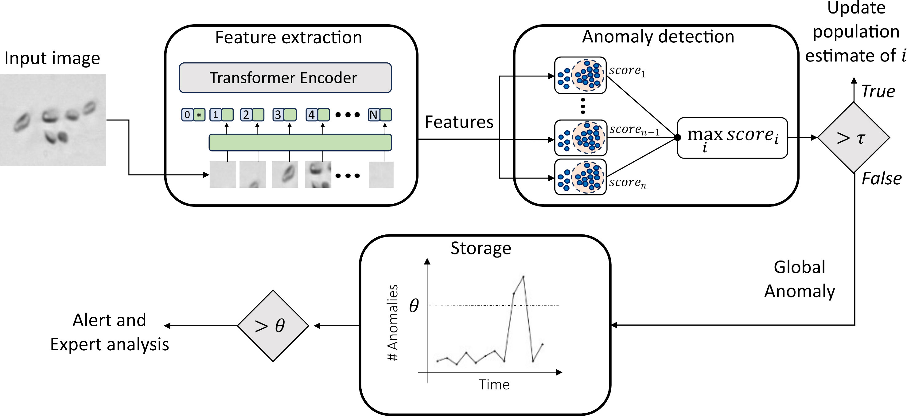
Figure 1 Schematic representation of the pipeline proposed to perform environmental monitoring with plankton.

In the following paragraph, we provide more details about each of the three components of the proposed method.

2.1 Feature extraction and compression

Our main idea is to detect and quantify plankton response to environmental threats as significant deviations from the average appearance of plankton microorganisms, inferred from acquired images. To support this objective, the first phase of the proposed approach consists in the extraction of highly discriminative features for plankton images, capable of detecting changes in the visual characteristics of planktonic images with the highest possible resolution.

Inspired by recent works (Salvesen et al., 2022; Alfano et al., 2022; Maracani et al., 2023; Pastore et al., 2023), we exploit a transfer learning framework to extract our set of phytoplankton descriptors. In such an approach, a large-scale dataset (source) is used to learn knowledge that is later transferred to the dataset of interest (target). We adopt a Vision Transformer (ViT-L16) pre-trained on ImageNet22K as a feature extractor, resulting in 1024 deep features per image. Additionally, we reduce the dimensionality of the obtained descriptors with PCA, in an attempt to temper the curse of dimensionality (Bellman, 1966; Verleysen and Francois, 2005).

2.2 Anomaly detection

The deep features extracted by means of the pre-trained Vision Transformer are used for training a set of anomaly detection algorithms. We train a separate detector for each class available in the training set. The trained detectors are later organized into a parallel architecture, and during testing, each test image is fed to every individual anomaly detector. Each anomaly detector provides a membership score corresponding to the fed image. At this stage, we have two possible outcomes: (i) the maximum score is higher than or equal to a threshold τ. In this case, the image is classified as belonging to the class corresponding to the detector, and the population counts for that class are updated (ii) the maximum score is lower than a threshold τ. The test image is rejected, labeled as a global anomaly, and stored for further analysis. See Sec. 3.3.1 for more details on the investigated anomaly detection algorithms. The threshold τ is an important hyperparameter, that we tune with an automatic procedure. See section 3.2.3 for more details.

2.3 Anomaly storage and alert

The detected global anomalies are stored and anomaly counting is updated. The number of anomalies as well as the evolution of population counts in time can be regarded as measurable feedback for the environmental monitoring task objective of our work. Describing the engineering framework for measuring the designed feedback is out of the scope of this work. However, we envision the possibility of setting an automatic alert when the anomaly frequency is higher than a threshold, that may be set by field experts through preliminary in situ tests. Images triggering anomalies are stored as well, allowing offline expert analyses to get better insights from the generated alerts.

2.4 Evaluation metrics

Our approach is based on the concept of anomaly detection, where one anomaly detector is trained for each distinct class available in the training set. Therefore the performances of our method can be measured through binary evaluation metrics. Specifically, given a sample belonging to training class k, we identify two possible outcomes: (i) the sample is recognized by the detector A_k(it brings the maximum membership score in the anomaly detector k, and such score is higher than the threshold τ, see Sec. 2.2). In this case, the sample is regarded as a True Positive (TP); (ii) the sample is rejected by all the trained detectors and it is treated as a False Negative (FN).

At this stage, we employ a leave-one-out approach, removing the detector A_kfrom our parallel architecture for each training class k, with two additional outcomes: (iii) the sample is recognized as in class by any of the remaining anomaly detectors. We refer to this sample as a False Positive (FP); (iv) the sample is correctly rejected by all the detectors. In this case, the sample is labeled as a True Negative (TN).

Therefore, exploiting the TP, FP, FN and TN definitions provided above, we select the Sensitivity (True Positive Rate or TPR), the Specificity (True Negative Rate or TNR) and the False Negative Rate (FNR) as reference metrics for our method, computed as described in Equations 1-3:

$\begin{array}{ll}\text{Sensitivity }(\text{TPR}):=\frac{\text{True Positives}}{\text{Total Number of Positive Samples}}=\frac{\text{TP}}{\text{TP }+\text{ FN}}& (1)\end{array}$

$\begin{array}{ll}\text{Specificity }(\text{TNR}):=\frac{\text{True Negatives}}{\text{Total Number of Negative Samples}}=\frac{\text{TN}}{\text{TN }+\text{ FP}}& (2)\end{array}$

$\begin{array}{ll}\text{FNR }:=\frac{\text{False Negatives}}{\text{False Negatives }+\text{ True Positives}}=\frac{\text{FN}}{\text{FN }+\text{ TP}}& (3)\end{array}$

It is worth noticing that a last important source of errors is represented by misclassified samples, that is, samples recognized by the incorrect anomaly detector. The rate of such misclassifed samples can be obtained from the described metrics, as 1 - (Sensitivity + FNR). In the computation of sensitivity, the FN include both the misclassified and the uncorrectly rejected samples.

3 Experiments

3.1 Datasets description

In this section, we describe the datasets we employed in this work for training the components of our pipeline, testing overall performance, and assessing the effectiveness of the proposed approach.

The images we used for our experiments come from the WHOI-Plankton Dataset (Sosik and Brownlee, 2015), a large-scale dataset containing grayscale microscopic plankton images from 103 different classes, acquired with IFCB by the Woods Hole Oceanographic Institute. We exploit two publicly available subsets commonly used as benchmarks in the plankton image analysis community: WHOI22 and WHOI40 (Sosik and Olson, 2007; Orenstein and Beijbom, 2017; Lumini and Nanni, 2019; Pastore et al., 2020; Pastore et al., 2023).

The two subsets (Sections 3.1.1 and 3.1.2) are used to tune and evaluate the performance of the different anomaly detection algorithms we consider in our analyses and to select the most appropriate number of principal components to retain for the dimensionality reduction of the deep pre-trained features.

Additionally, we manually extract a selection of phytoplankton images from the full WHOI dataset belonging to different years of acquisitions, with the aim of analyzing the evolution in time of a microorganism reference population. A detailed description of the obtained set can be found in Section 3.1.3. Sample images for the three datasets used in our work are depicted in Figure 2.

Figure 2

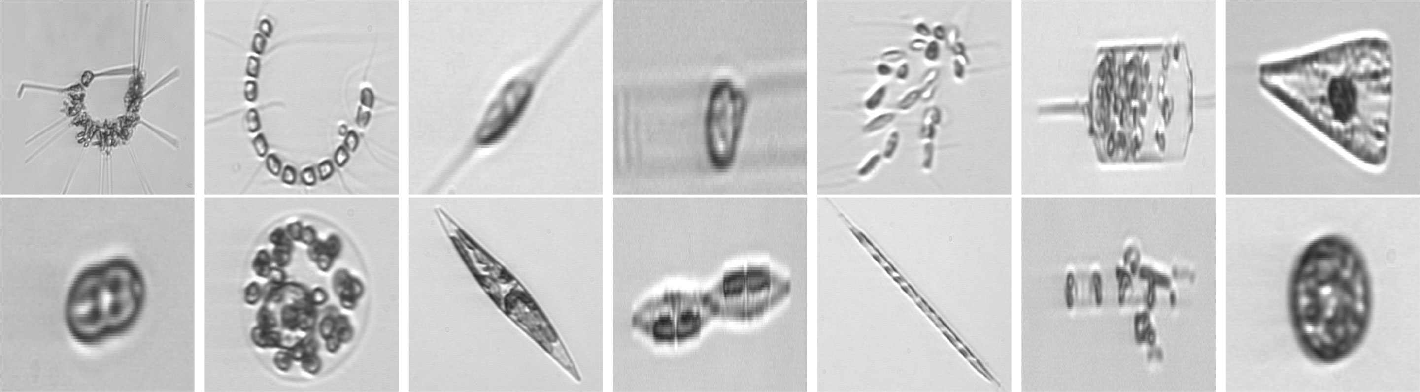
Figure 2 Images from WHOI15 (2007-2011), in their appearance once square-resized to become compatible input for deep neural networks. One example for each distinct class is depicted. From upper left to bottom right: Asterionellopsis, Chaetoceros, Cylindrotheca, Dactyliosolen, Dinobryon, Ditylum, Licmophora, pennate, Phaecystis, Pleurosigma, Pseudonitzschia, Rhizosolenia, Skeletonema, Thalassiosira. Images from WHOI22 and WHOI40 come from the same superset, the WHOI-Plankton dataset, and exhibit a similar appearance.

3.1.1 WHOI22

WHOI22 constitutes a set of planktonic images gathered between 2005 and 2006 at the Woods Hole Oceanographic Institute, subsequently published in 2007 (Sosik and Olson, 2007). This collection encompasses 22 distinct categories of phytoplankton, containing 300 instances per category. The images are presented in grayscale and vary in dimensions. The dataset is partitioned into two sets: a training set and a test set, each comprising 3,300 samples (150 images for each category), summing up to a total of 6,600 data points. It is worth noting that this dataset is characterized by a fine granularity between different classes, coupled with its exceptional image quality owing to the high-quality acquisitions, which capture intricate morphological particulars.

3.1.2 WHOI40

WHOI40 refers to a specific subset introduced in Pastore et al. (2020), composed of phytoplankton image acquisitions primarily spanning the period from 2011 to 2014. This set provides 40 distinct categories (some of which align with those found in the WHOI22 dataset) for a total of 4,086 samples. Similar to WHOI22, the images are in grayscale and come with varying dimensions, but a predefined test set is not available. This dataset is not as fine-grained as WHOI22, but provides many more classes and therefore it brings different challenges to overcome.

3.1.3 WHOI15 (2007-2010)

In this work, we build a phytoplankton image dataset from the available WHOI large-scale collection, considering samples acquired across four years, from 2007 to 2010. Among the 22 classes available in the WHOI22 dataset, we observe that 15 of them appear with a sufficient number of samples for each of the acquisition years between 2007 and 2010. Specifically, this is observed for the classes labeled as Asterionellopsis, Chaetoceros, Cylindrotheca, Dactyliosolen, Detritus, Dinobryon, Ditylum, Licmophora, Pennate, Phaeocystis, Pleurosigma, Pseudonitzschia, Rhizosolenia, Skeletonema, Thalassiosira. From the 15 classes, we randomly pick a maximum of 500 images, for each class and for each year in that specific time span. With this procedure, we obtain a single dataset that is the union of four different sets, one for each year in the period 2007-2010.

The final dataset has a total of 24,666 images, with an uneven distribution across classes and years. Regarding the number of samples per year, 5841 samples come from 2007, 6323 from 2008, 6696 from 2009, 5,806 from 2010. The exact number of images per class and year are represented as histograms in the Supplementary Material.

3.2 Experiment details

The software implementation of the experiments supporting the proposed methodology is realized using the Python programming language (Python Software Foundation, 2023), with the aid of dedicated machine-learning and deep-learning libraries and frameworks.

Specifically, the deep neural networks adopted in this work are implemented in PyTorch (Paszke et al., 2019), while the weights learned through pre-training the networks on ImageNet come from both Torchvision and TIMM models repositories (Maintainers and Contributors, 2016; Wightman, 2019).

Regarding the anomaly detectors and PCA routines, we rely on the scikit-learn library (Pedregosa et al., 2011), which provides efficient and reliable implementations of many state-of-the-art machine learning algorithms. Generic numerical computing operations and data manipulation are implemented with the aid of NumPy (Harris et al., 2020) and Pandas (Pandas Development Team, 2023).

The following dedicated subsections discuss the experimental setup regarding feature extraction and the training and testing of our pipeline’s components.

3.2.1 Feature extraction

Images belonging to the dataset of interest are first resized to a 224x224 pixel resolution and normalized to obtain input RGB values between 0 and 1, in order to render them compatible with the input requirements of the available pre-trained deep neural networks. Additionally, they are also standardized with respect to the RGB color distribution of ImageNet, as in transfer-learning scenarios we desire to shift input image distribution closer to the one learned by the deep neural network during its pre-training. This is obtained by subtracting ImageNet’s RGB color mean from input images and further dividing their values by ImageNet’s standard deviation. At this stage, images are ready to be fed to the deep feature extractor, which is obtained by removing the fully-connected classification-head from the original model. Given a set of N input images, the deep feature extractor produces a feature vector $\varphi \in {ℝ}^D$ for each of them (with D usually in the order of 10³), resulting in a final set of deep pre-trained features $\text{Φ }\in {ℝ}^{N\times D}$ . Before actually performing feature extraction, we gather three separate sets of images X_tr, X_valand X_te: in the case of WHOI22, the test set corresponds to the already pre-defined test set, while for WHOI40 and WHOI15 (2007-2010), we hold-out (Yadav and Shukla, 2016) 20% of samples as a test set, performing an additional hold-out with an 80/20 ratio, to separate a proper validation set from the remaining images. We then obtain three sets of deep pre-trained features by feeding the three disjointed sets X_tr, X_val and X_teto the deep feature extractor, Φ_tr, Φ_val and Φ_te. As a final step before applying dimensionality reduction to these sets of features, we first proceed to apply min-max normalization and standardization, extracting the normalization values from Φ_tr.

3.2.2 Dimensionality reduction

The three sets of deep pre-trained features Φ_tr, Φ_val and Φ_te undergo dimensionality reduction through PCA, for which we retain the first 50 principal components. The associated linear projection is computed from the training data by fitting PCA on Φ_tr and then we apply it to Φ_tr, Φ_val and Φ_te. By doing so, we obtain the final features that are used for training and evaluating the anomaly detectors. We indicate such features as $Z_{tr}\in {ℝ}^{N\times 50}$, $Z_{val}\in {ℝ}^{N\times 50}$ and $Z_{te}\in {ℝ}^{N\times 50}$. In order to test the importance of this specific step and to search for the best possible number of components, we run our analyses also with the plain deep pre-trained features coming from the employed neural network without any kind of compression, and we test several alternatives for the number of components to retain as well. Details on this particular step are outlined in Section 3.3.3.

3.2.3 Training and evaluation

As we are dealing with datasets equipped with labels provided by field experts, our data includes also an associated vector Y containing integer values associated with the class to which each sample belongs. In our case, the pre-trained deep features with reduced dimensionality Z_tr belonging to the extracted training set, are used alongside their associated label vectors Y_tr to train one anomaly detector per each available class. If the dataset has K classes we instantiate K anomaly detectors, denoted as {A_k| k ∈ [1,K]}, and each detector A_k is trained only on the z_i∈ Z_tr such that Y_tri= k. In our approach, a test image is fed to the set of trained anomaly detectors A. From each anomaly detector, we extract the membership score, exploiting the decision function method in the scikit-learn implementation (e.g., the signed distance to the separating hyperplane, in the case of the one-Class SVM). The maximum anomaly score is selected, and if it is higher than or equal to a threshold τ, the sample is assigned to the corresponding class, otherwise it is identified as a global anomaly and stored for further analyses or computations. The threshold τ is tuned with the following automatic procedure, exploiting the extracted validation set Φ_val. Ideally, the higher the threshold, the higher the Specificity, and vice-versa. Thus, we perform a grid search to identify the best trade-off between Sensitivity and Specificity. We evaluate candidate thresholds in the interval [−1,1] with a step of 0.05. The negative samples to measure the Specificity are obtained with a leave-one-out approach. Thus, for each of the available classes k and for each of the candidate thresholds, we measure the Sensitivity, as the number of samples belonging to class k correctly detected by the anomaly detector A_k as in class, and the Specificity, corresponding to the number of samples belonging to k rejected when only the remaining anomaly detectors $\left\{A_j|j\ne k\right\}$ are considered. The threshold τ is then selected as the one minimizing the absolute difference between the average Sensitivity and the average Specificity.

3.3 Results

In this section, we highlight and comment on the results obtained throughout our experiments. This includes also the intermediate results regarding the tuning of the hyperparameters, as well as the final measured performances on all the considered datasets, including the proposed test ranging through different years of acquisition.

3.3.1 Performance evaluation across different anomaly detection algorithms

The anomaly detection algorithm is a core element of the proposed approach. We consider four different algorithms, LocalOutlierFactor (LoF) (Breunig et al., 2000), Isolation Forest (IFO) (Liu et al., 2008), Robust Covariance estimator (RC) (Rousseeuw and Driessen, 1999), and One-Class SVM (Scholkopf et al., 1999) (with a Radial Basis Function kernel Vert et al., 2004), comparing them in terms of performances on the WHOI22 and the WHOI40 datasets, in the experimental setting previously described. A crucial parameter shared by the evaluated methods is the contamination factor, which controls the prior knowledge regarding the proportion of out-of-distribution samples among training data. The contamination amount is selected among five possible different values, namely: 1%, 5%, 7.5%, 10%, and 15%, choosing the value that maximizes the performances on the validation set. Table 1 shows the obtained results on the WHOI22, while Table 2 reports the results corresponding to the WHOI40 dataset.

Table 1

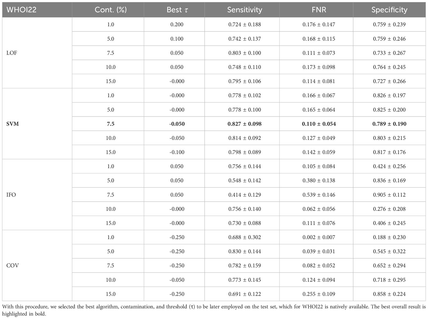
Table 1 Performance across different anomaly detection algorithms and contamination parameters on a hold-out validation set from the training set of the WHOI22 dataset.

Table 2

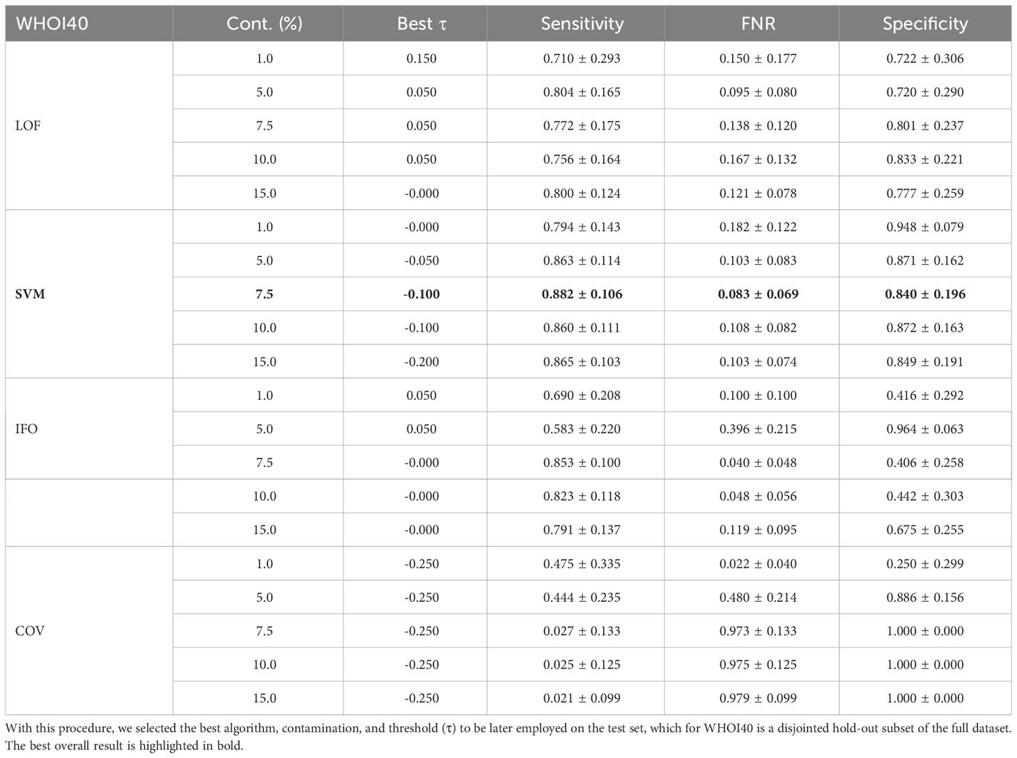
Table 2 Performance across different anomaly detection algorithms and contamination parameters on a hold-out validation set from the WHOI40 dataset.

The one-class SVM algorithm with a contamination parameter equal to 0.075 overall brings the best average performances (with respect to the training classes) for both validation splits of the two datasets (see Tables 1, 2). For this reason, we use the one-class SVM with a contamination parameter of 0.075, while τ is set to τ = −0.05 for WHOI22 and to τ = −0.10 for WHOI40. This configuration brings the test performances reported in Table 3, corresponding to a Sensitivity of 0.839 for WHOI22 and 0.870 for WHOI40. We also report a score of 0.094 for WHOI22 and 0.085 for WHOI40 in terms of FNR, while Specificity reaches 0.782 and 0.840 for the two datasets respectively.

Table 3

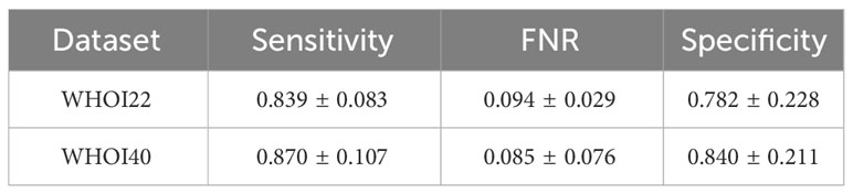
Table 3 Results of the best configurations for the test sets of the two datasets, WHOI22 and WHOI40.

3.3.2 Impact of the deep feature extractor on the performance

We perform a comparative study on the deep feature extractor used to obtain the set of descriptors fed to the anomaly detectors. Our objective is to empirically prove that the pre-trained ViTL-16 used in this study as a feature extractor leads to the best performances, in terms of highest anomaly detection accuracy when used as input, compared to other deep neural networks. In detail, we compare Sensitivity, FNR, and Specificity on our target datasets, when using different pre-trained deep neural networks to extract features representing the input to the one-class SVM anomaly detectors. We compare four ImageNet-1K pre-trained CNNs, namely MNASNet 1.3 (Tan et al., 2019), ResNet101 (He et al., 2015), EfficientNetB1 (Tan and Le, 2019), DenseNet201 (Huang et al., 2016), three ImageNet-1K pre-trained Vision transformers (SwinV2-T (Liu et al., 2021), DeiT-B (Touvron et al., 2021), and ConViTB (d’Ascoli et al., 2021)), and a vision transformer pre-trained on ImageNet-22k (ViT-L16 (Dosovitskiy et al., 2020), our selected model), with Tables 4, 5 reporting the obtained results. The ViTL-16 pre-trained transformer provides the best representation. In the case of WHOI22, it brings an improvement in Sensitivity of 1.7% over the DenseNet-201, and of 6% in Specificity over ConViT-B, which are the second best-performing models in terms of the two individual metrics. Considering the performances on WHOI40, DenseNet-201 is the second best-performing model in terms of both Sensitivity and Specificity but the ImageNet-22k pre-trained ViTL-16 achieves a 1% higher Sensitivity, and a sensible improvement in Specificity of 13% over the best-performing alternative.

Table 4

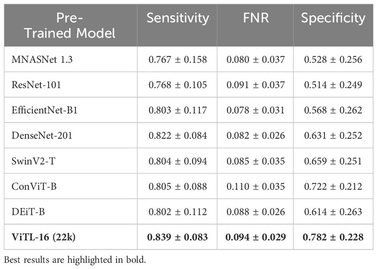
Table 4 Ablation on WHOI22 regarding the best pre-trained model for deep feature extraction.

Table 5

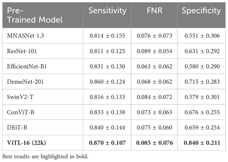
Table 5 Ablation on WHOI40 regarding the best pre-trained model for deep feature extraction.

3.3.3 Ablation study on dimensionality reduction

In our experiments, we involve the usage of a PCA dimensionality reduction algorithm with 50 components. In this section, we provide an ablation study to empirically experiment with the impact of dimensionality reduction on performance. We test the usage of the original deep pre-trained features, as well as different numbers of principal components used for projecting features in the associated lower-dimensional space, on our target datasets. Specifically, we compare Sensitivity, FNR, and Specificity when using the plain features extracted from the ViTL-16 encoder, with dimensionality equal to 1024, and the features obtained through PCA reduction with a number of principal components varying between 10 and 200, as input for the one-class SVM anomaly detectors. The performances measured in our experiments are outlined in Table 6 for the WHOI22 dataset and (Table 7) for the WHOI40 one. A PCA with 50 components is confirmed to lead to the best performances for both datasets.

Table 6

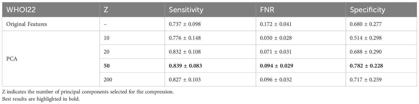
Table 6 Ablation on Feature Compression algorithm and impact of dimensionality reduction on performances for the WHOI22 dataset.

Table 7

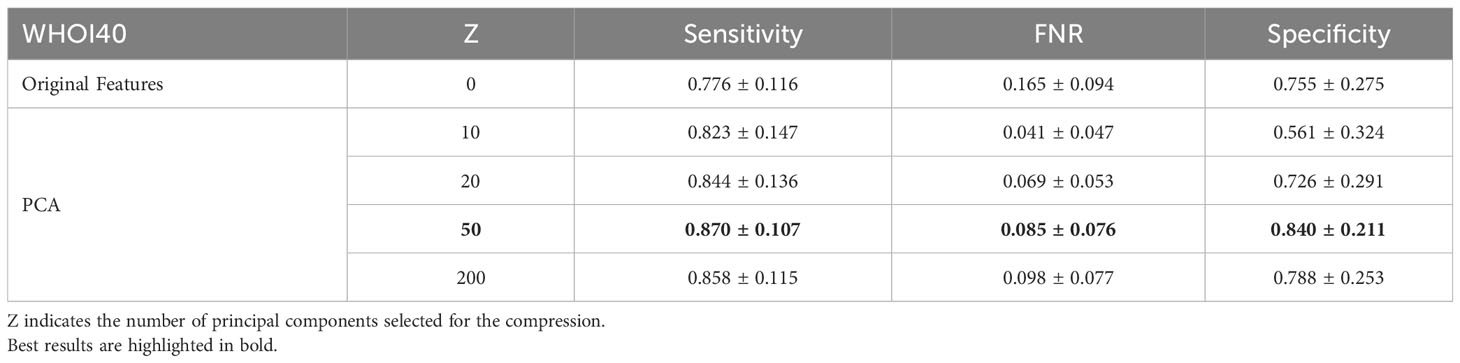
Table 7 Ablation on Feature Compression algorithm and impact of dimensionality reduction on performances for the WHOI40 dataset.

3.3.4 Comparison with state-of-the-art multi-class classification methods

WHOI22 is a popular benchmark dataset exploited in several works focusing on plankton image classification (Lumini and Nanni, 2019; Kyathanahally et al., 2021; Maracani et al., 2023). Even if the general framework of classification is different from the one faced in this work, in this paragraph we provide a comparison in an attempt to frame our results with respect to the existing state-of-the-art. To do so, it is possible to focus only on the Sensitivity, which measures the correct predictions per class, ignoring the results of the leave-one-out approach that is instead used to evaluate the Specificity (i.e., to measure the number of correctly predicted anomalies). Exploiting different ensembles of CNNs or transformers, in Maracani et al. (2023) the authors report a test accuracy of 0.966 on the WHOI22, while in Kyathanahally et al. (2021) a value of 0.961 is obtained, and (Lumini and Nanni, 2019) reports a test accuracy of 0.958. With a sensitivity of 0.839, our method shows a drop of ∼ 12% with respect to state-of-the-art classification accuracy. This is somehow expected, bearing in mind that in our experiments we tune our algorithm’s components to balance the trade-off between Sensitivity and Specificity. The aim of our work is in fact not to maximize the multi-class classification performance, but rather to design a method capable of detecting anomalies in a feature space of reference, starting from phytoplankton images, while maintaining a reasonable classification performance. Additionally, it is worth underlining that in Lumini and Nanni (2019); Kyathanahally et al. (2021); Maracani et al. (2023), the authors use ensembles of at least four deep neural networks, that need to be trained on the target plankton image dataset. In our work, instead, we use a single pre-trained transformer as a feature extractor (with no further training), and we only train one anomaly detector per class, significantly reducing the computational burden of the proposed method.

3.3.5 Temporal analysis through anomaly detection in feature space

Our best-performing pipeline involves the usage of one-class SVM anomaly detectors, with input represented by the 50 principal components computed on ImageNet-22K pre-trained ViTL-16 features extracted from plankton images. At this stage, we exploit the WHOI15 dataset to test the ability of the proposed approach to generalize over time. In this dataset, we select 15 classes that are acquired for 4 consecutive years in the large-scale WHOI dataset (see Sec. 3.1.3). Thus, we can test the performance of our pipeline across time in a realistic scenario, where the same classes are acquired across different years. This experiment is helpful to have insights into the natural in-time variability of a group of interesting classes, and we expect our anomaly detection algorithms to be able to recognize with reasonable accuracy samples of their respective class, even if they are acquired in different years with respect to the ones used for training. We train a single one-class SVM algorithm for each of the 15 available classes for each one of the 4 years of the acquisition included in the dataset we built, and we perform the automatic extraction of a dedicated threshold τ for each year on the respective validation sets. Later, we test the trained algorithms on the test set extracted from the year corresponding to the training samples, and for each one of the available subsequent years. For instance, for images acquired in 2008, we train the detectors on the 2008 training set, we derive τ from 2008’s validation set, and evaluate the performance on the test data acquired in the same and the following years (2008, 2009, and 2010). Table 8 shows the obtained results.

Table 8

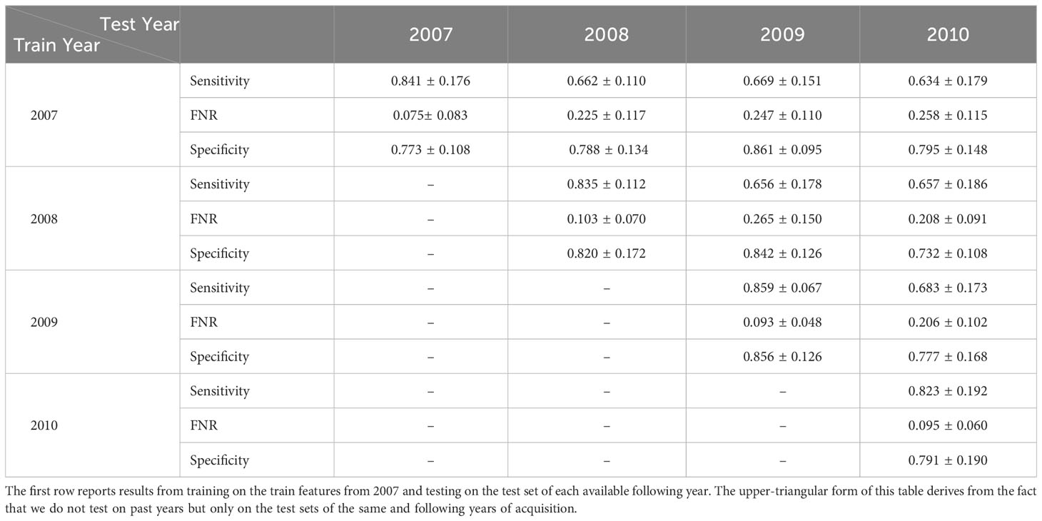
Table 8 Average Sensitivity, FNR, and Specificity of the parallel OneClass-SVMs trained on the reduced deep pre-trained features coming from WHOI10 from different years and tested on the same type of features extracted from images coming from subsequent years of WHOI’s acquisitions, starting from 2007 up to 2010.

In experiments in which the training year and the testing year coincide, we can see that the performances are comparable with those obtained on WHOI22 and WHOI40. This is indicated on the diagonal of (Table 8), where Sensitivity has a minimum of 0.82 in 2010 and a maximum of 0.859 in 2009. Regarding Specificity, we can observe a minimum of 0.773 in 2007 and a maximum of 0.856 in 2009, while FNR is close to 0.10, with a minimum of 0.075 in 2007. A drop in Sensitivity is observed when the test year differs from the training one. This is somewhat to be expected due to the distribution shift in the images across time. Among the multiple possible reasons, we can include per-class populations, which are not the same for all classes across years, naturally occurring fluctuations that may be hard to infer from a single year of training, as well as potential factors related to the acquisition system.

The highest drop involves the experiment in which the detectors are trained on images from 2007 and tested on 2010 corresponding to a decrease of 0.21 in Sensitivity. For the other training years, the drops in Sensitivity are around 0.18, with an average Sensitivity always above 0.65. The decrease in Sensitivity is associated with an increase in the FNR, generally ranging between 0.20 and 0.25 in tests run on subsequent years. Specificity, instead, shows little differences over time or even improves in some cases, suggesting that the pipeline is able to correctly recognize the presence of completely novel objects and instances with respect to the training set.

To give more insights into the individual classes and distribution shifts across years, we perform an experiment where we train our anomaly detection algorithm on a joint dataset including years 2007, 2008, and 2009, while testing on the samples from 2010. In this experiment, we obtain an average Sensitivity of 0.768, 0.135 in FNR, and an average Specificity of 0.725, improving significantly the overall performances on the unseen year with respect to the previous experiments. The lowest Sensitivity is measured for the class Ditylum, confirming the behavior observed in the results reported in Figure 3. Regarding the Specificity, the most problematic classes are Skeletonema and Thalassiosira, similarly to what obtained with the individual years experiments. Nonetheless, the increase in Sensitivity suggests that a more diverse set of examples and periodic retraining with more recent acquisitions may be helpful to keep the system up to date with respect to the naturally occurring modifications in the observed populations.

Figure 3

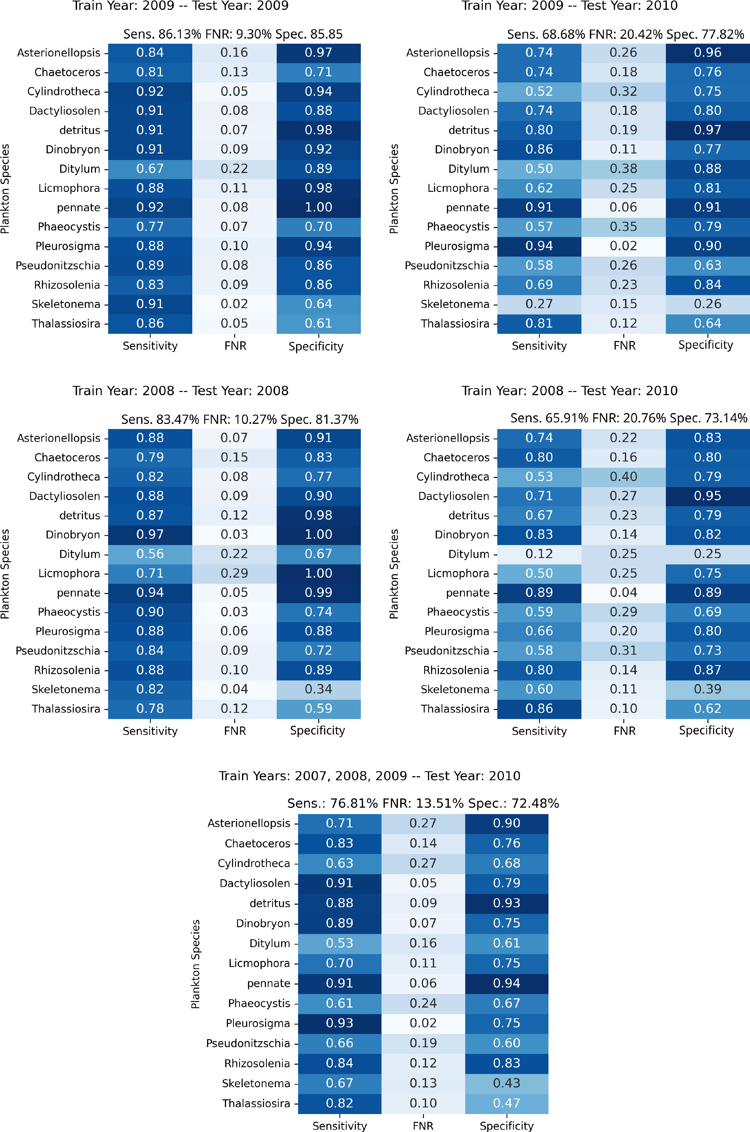
Figure 3 Per-class performances of the proposed approach in the experiments involving the WHOI15 dataset, simulating different years of acquisition and testing. Top Left, Top Right, Middle Left, and Middle Right depict experiments in which training and test procedures involve single years; the specific years are outlined in the upper part of each figure. Bottom: Results from training on the years 2007, 2008, and 2009, while testing on features extracted from 2010 acquisitions, simulating the accumulation of samples through time in order to test on newly acquired data.

4 Discussion

Plankton organisms can play an important role in assessing environmental perturbations, as they react to even slight changes in the environment with physiological modifications in morphology and behavior. In this work, we propose a machine learning framework to perform anomaly detection in phytoplankton images, with the aim to support the detection of perturbations in the environment by monitoring changes in the microorganisms’ morphology. We propose a method based on anomaly detection algorithms, trained on top of deep pre-trained features, extracted by means of a vision transformer pre-trained on ImageNet22K. Assuming an initial training set is available, we first design a parallel architecture composed of one anomaly detection algorithm per available class. When a test image is fed to each of the detectors, we select the detector providing the maximum membership score. If such score is above an automatically determined threshold, we consider the sample as in class, and update the population count for the corresponding class. Otherwise, we treat the sample as a global anomaly, storing it for further analysis and updating the anomaly count. At this stage, we propose to exploit our approach to suggest potential critical situations, which may be related to environmental perturbations, by using a threshold on the number of global anomalies per time. This threshold is likely to depend on the specific site of sample acquisition, and needs to be tuned by experts in the field. We perform comparative studies on the deep feature extractor and different anomaly detectors in terms of performances on two publicly available benchmark datasets, the WHOI22 (Sosik and Olson, 2007), and the WHOI40 (Pastore et al., 2020). Our experiments show that the best performances correspond to the adoption of a one-class SVM algorithm trained on top of the first 50 principal components computed on features extracted with a ViTL-16 pre-trained on ImageNet22K. The usage of a pre-trained neural network for feature extraction makes our approach very efficient, as the only training process regards the anomaly detectors. To provide a reference on the time needed for the computation, we consider the experiments on the WHOI22 dataset. The feature extraction with ViTL-16 requires an average of 0.032 ± 0.003 seconds per image, while the detectors average training time per class, is 6.26 ± 2.62 milliseconds. The computational times are averaged among 10 different runs, on a laptop with AMD Ryzen 9 6900 HS, with 16 GB of RAM and a GPU NVIDIA RTX 3080, with 8 GB of VRAM. Feature extraction is performed on the GPU.

We then build a dataset containing 15 classes acquired from 2007 to 2010 in the WHOI large-scale dataset (Sosik and Brownlee, 2015), which we refer to as WHOI15. Our aim is to exploit the WHOI15 to evaluate the generality of our solution across samples acquired in different years. Thus, we train our pipeline on the images acquired in one year, evaluating the performances on the test set of the same year and the data acquired in the following years. A drop in Sensitivity is observed, in general, when testing on classes acquired across different years, with no impact on the Specificity, evaluated with a leave-one-out approach. The performances are similar to the benchmark datasets (WHOI22 and WHOI40) when our method is trained on the training set of one year, and tested on the test set corresponding to the same year. We hypothesize that the drop in Sensitivity across different years may be related to natural fluctuations, difficult to infer from a single year of training, as well as potential changes related to the water conditions and the acquisition system. Nonetheless, the average Sensitivity has a minimum value of 0.63, with a high deviation with respect to individual classes (see Table 8). A limitation of the dataset used in this work is the relatively low number of available images per class, with a severe imbalance in some years of acquisition. The highest number of images for training is 400 per class (with a minimum of 36, see Supplementary Material for more details), which is likely not enough for actually covering intra-class variance in appearance, which may be high for specific classes. To further investigate in this direction, we perform an experiment where the 2010 samples are used for testing, and the remaining years’ images are used for training. We select the 2010 dataset as a test because it shows the highest drop in Sensitivity in our previous experiment. We obtain a significant improvement in average Sensitivity, and a general trend more similar to the single-year experiment, where training and evaluation are performed on the same year. These results suggest that periodic re-training and cumulating training samples across time could help maintain high performances in the designed method. Nonetheless, some classes still show a drop in Sensitivity (e.g., Ditylum) or Specificity (e.g., Skeletonema and Thalassiosira) with respect to the average. Exploring the images of these classes, we realized that they are more blurred and less detailed in the 2010 dataset than in the other years of acquisition.

Regarding the aim of the designed method, it is worth stressing that our anomaly detection approach intends to detect significant variations of phytoplankton images in a feature space of reference. However, such deviations can be related to different sources, including novel classes (not included in the initial training set), plankton morphological modifications due to environmental changes, and a possible source of errors caused by image distortions or noise. Yet, an automatic disentanglement of the different sources of anomalies is not possible with our proposed approach. However, we sketch a possible pipeline to handle the different sources of anomalies. First, we propose to measure the average number of anomalies in a certain period of time and situ of acquisition. We can indeed expect a systematic amount of errors related to image distortions or noise, or simply related to intrinsic algorithm mistakes, in such a period of time. For this reason, we propose to set a threshold on the number of detected anomalies with respect to the average number of anomalies per time. Only if the number of anomalies is higher than this threshold, an alert should be emitted. At this point, we envision a human in the loop that can manually identify signaled anomalies. As further support for the human expert, a possibility could be to group the features corresponding to the anomalies using clustering algorithms, as the one described in Pastore et al. (2023), where plankton images are shown to be clustered with high accuracy. Sample images belonging to each of the detected clusters could be reviewed by the expert, providing a label, that can be used to train new anomaly detectors, in the case of novel classes. Finally, in this work we focus on phytoplankton microscopic images acquired with IFCB. However, it’s worth underlining that plankton image analysis may include several subdomains and imaging devices over phytoplankton and IFCB, for instance, zooplankton images acquired with diverse acquisition systems and modalities, such as silhouette grayscale images acquired with the In Situ Ichthyoplankton Imaging System (ISIIS) (Cowen et al., 2015), grayscale scan images collected with ZooScan (Elineau et al., 2018), and color dark field images obtained with devices as the Scripps Plankton Camera (SPC) (Orenstein et al., 2020b), and the Imaging Plankton Probe (IPP) (Li et al., 2021), just to name a few. We expect our method and designed pipeline to be in general applicable to such different sources and types of images, nonetheless, further experiments and tests are required to assess the generality and the specific performances of the proposed anomaly detection approach with respect to the identified domains.

Even if further research is necessary to prove the accuracy of the proposed approach in actually detecting plankton responses related to changes in the environment, we believe that this work may be a stepping stone towards the fundamental aim of using plankton as a biosensor, supporting the detection of potentially critical situations and environmental perturbations.

Data availability statement

Publicly available datasets were analyzed in this study. This data can be found here: https://hdl.handle.net/10.1575/1912/7341. The WHOI15 dataset, as well as the code needed for reproducing our results are available at: https://github.com/Malga-Vision/Anomaly-detection-in-feature-space-for-detecting-changes-in-phytoplankton-populations.

Author contributions

MC: Data curation, Investigation, Methodology, Software, Validation, Visualization, Writing – original draft. FO: Funding acquisition, Investigation, Methodology, Supervision, Validation, Visualization, Writing – original draft. VP: Conceptualization, Funding acquisition, Investigation, Methodology, Project administration, Supervision, Validation, Visualization, Writing – original draft.

Funding

The author(s) declare that no financial support was received for the research, authorship, and/or publication of this article.

Acknowledgments

VP was supported by FSE REACT-EU-PON 2014–2020, DM 1062/2021, COD. 11-G-14987-1.

Conflict of interest

The authors declare that the research was conducted in the absence of any commercial or financial relationships that could be construed as a potential conflict of interest.

Publisher’s note

All claims expressed in this article are solely those of the authors and do not necessarily represent those of their affiliated organizations, or those of the publisher, the editors and the reviewers. Any product that may be evaluated in this article, or claim that may be made by its manufacturer, is not guaranteed or endorsed by the publisher.

Supplementary material

The Supplementary Material for this article can be found online at: https://www.frontiersin.org/articles/10.3389/fmars.2023.1283265/full#supplementary-material

References

Alfano P. D., Rando M., Letizia M., Odone F., Rosasco L., Pastore V. P. (2022). “Efficient unsupervised learning for plankton images,” in 2022 26th international conference on pattern recognition (ICPR) (IEEE), 1314–1321.

Google Scholar

Bellman R. (1966). Dynamic programming. Science 153, 34–37. doi: 10.1126/science.153.3731.34

PubMed Abstract | CrossRef Full Text | Google Scholar

Benfield M. C., Grosjean P., Culverhouse P. F., Irigoien X., Sieracki M. E., Lopez-Urrutia A., et al. (2007). Rapid: research on automated plankton identification. Oceanography 20, 172–187. doi: 10.5670/oceanog.2007.63

CrossRef Full Text | Google Scholar

Breunig M. M., Kriegel H.-P., Ng R. T., Sander J. (2000). Lof: Identifying density-based local outliers. SIGMOD Rec. 29, 93–104. doi: 10.1145/335191.335388

CrossRef Full Text | Google Scholar

Brierley A. S. (2017). Plankton. Curr. Biol. 27, R478–R483. doi: 10.1016/j.cub.2017.02.045

PubMed Abstract | CrossRef Full Text | Google Scholar

Cowen R. K., Sponaugle S., Robinson K. L., Luo J., Oregon State University, et al. (2015). Planktonset 1.0: Plankton imagery data collected from f.g. walton smith in straits of florida from 2014-06-03 to 2014-06-06 and used in the 2015 national data science bowl (ncei accession 0127422). doi: 10.7289/V5D21VJD

CrossRef Full Text | Google Scholar

d’Ascoli S., Touvron H., Leavitt M. L., Morcos A. S., Biroli G., Sagun L. (2021). Convit: improving vision transformers with soft convolutional inductive biases. J. Stat. Mechanics: Theory Experiment 2022, 2286–2296. doi: 10.1088/1742-5468/ac9830

CrossRef Full Text | Google Scholar

Dosovitskiy A., Beyer L., Kolesnikov A., Weissenborn D., Zhai X., Unterthiner T., et al. (2020). An image is worth 16x16 words: Transformers for image recognition at scale

Google Scholar

Elineau A., Desnos C., Jalabert L., Olivier M., Romagnan J.-B., et al. (2018). Zooscannet: plankton images captured with the zooscan. doi: 10.17882/55741

PubMed Abstract | CrossRef Full Text | Google Scholar

Gönen M., Alpaydın E. (2011). Multiple kernel learning algorithms. J. Mach. Learn. Res. 12, 2211–2268.

Google Scholar

González P., Álvarez E., Díez J., López-Urrutia Á. (2017). and del coz, J Validation methods for plankton image classification systems. J.Limnology Oceanography: Methods 15, 221–237.

Google Scholar

Hanazato T. (2001). Pesticide effects on freshwater zooplankton: an ecological perspective. Environ. pollut. 112, 1–10. doi: 10.1016/S0269-7491(00)00110-X

PubMed Abstract | CrossRef Full Text | Google Scholar

Harris C. R., Millman K. J., van der Walt S. J., Gommers R., Virtanen P., Cournapeau D., et al. (2020). Array programming with numpy. Nature 585, 357–362. doi: 10.1038/s41586-020-2649-2

PubMed Abstract | CrossRef Full Text | Google Scholar

Hays G. C., Richardson A. J., Robinson C. (2005). Climate change and marine plankton. Trends Ecol. Evol. 20, 337–344. doi: 10.1016/j.tree.2005.03.004

PubMed Abstract | CrossRef Full Text | Google Scholar

He K., Zhang X., Ren S., Sun J. (2015). “Deep residual learning for image recognition,” in 2016 IEEE conference on computer vision and pattern recognition (CVPR), 770–778.

Google Scholar

Huang G., Liu Z., Weinberger K. Q. (2016). “Densely connected convolutional networks,” in 2017 IEEE conference on computer vision and pattern recognition (CVPR), 2261–2269.

Google Scholar

Kyathanahally S. P., Hardeman T., Merz E., Bulas T., Reyes M., Isles P., et al. (2021). Deep learning classification of lake zooplankton. Front. Microbiol. 12, 3226. doi: 10.3389/fmicb.2021.746297

CrossRef Full Text | Google Scholar

Li J., Chen T., Yang Z., Chen L., Liu P., Zhang Y., et al. (2021). Development of a buoy-borne underwater imaging system for in situ mesoplankton monitoring of coastal waters. IEEE J. Oceanic Eng. 47(1), 88–110. doi: 10.1109/JOE.2021.3106122

CrossRef Full Text | Google Scholar

Liu Z., Lin Y., Cao Y., Hu H., Wei Y., Zhang Z., et al. (2021). Swin transformer: Hierarchical vision transformer using shifted windows. 2021 IEEE/CVF Int. Conf. Comput. Vision (ICCV), 9992–10002. doi: 10.1109/ICCV48922.2021.00986

CrossRef Full Text | Google Scholar

Liu F. T., Ting K. M., Zhou Z.-H. (2008). “Isolation forest,” in Proceedings of the 2008 eighth IEEE international conference on data mining (USA: IEEE Computer Society), 413–422. doi: 10.1109/ICDM.2008.17

CrossRef Full Text | Google Scholar

Lombard F., Boss E., Waite A. M., Vogt M., Uitz J., Stemmann L., et al. (2019). Globally consistent quantitative observations of planktonic ecosystems. Front. Mar. Sci. 6. doi: 10.3389/fmars.2019.00196

CrossRef Full Text | Google Scholar

Lumini A., Nanni L. (2019). Deep learning and transfer learning features for plankton classification. Ecol. Inf. 51, 33–43. doi: 10.1016/j.ecoinf.2019.02.007

CrossRef Full Text | Google Scholar

Lumini A., Nanni L., Maguolo G. (2020). Deep learning for plankton and coral classification. Appl. Computing Inf 19, 265–283. doi: 10.1016/j.aci.2019.11.004

CrossRef Full Text | Google Scholar

Maintainers and Contributors (2016) Torchvision: Pytorch’s computer vision library. Available at: https://github.com/pytorch/vision.

Google Scholar

Maracani A., Pastore V. P., Natale L., Rosasco L., Odone F. (2023). In-domain versus out-of-domain transfer learning in plankton image classification. Sci. Rep. 13, 10443. doi: 10.1038/s41598-023-37627-7

PubMed Abstract | CrossRef Full Text | Google Scholar

Ohman M. (1988). Behavioral responses of zooplankton to predation. Bull. Mar. Sci. 43, 530–550.

Google Scholar

Orenstein E. C., Beijbom O. (2017). “Transfer learning and deep feature extraction for planktonic image data sets,” in 2017 IEEE winter conference on applications of computer vision (WACV) (IEEE), 1082–1088.

Google Scholar

Orenstein E. C., Kenitz K. M., Roberts P. L., Franks P. J., Jaffe J. S. (2020a). Semi-and fully supervised quantification techniques to improve population estimates from machine classifiers. Limnology Oceanography: Methods 18, 739–753. doi: 10.1002/lom3.10399

CrossRef Full Text | Google Scholar

Orenstein E. C., Ratelle D., Briseño-Avena C., Carter M. L., Franks P. J. S., Jaffe J. S., et al. (2020b). The scripps plankton camera system: A framework and platform for in situ microscopy. Limnology Oceanography: Methods 18, 681–695. doi: 10.1002/lom3.10394

CrossRef Full Text | Google Scholar

Pandas Development Team (2023). pandas-dev/pandas: pandas. doi: 10.5281/zenodo.8092754

CrossRef Full Text | Google Scholar

Pastore V. P., Ciranni M., Bianco S., Fung J. C., Murino V., Odone F. (2023). Efficient unsupervised learning of biological images with compressed deep features. Image Vision Computing 104764. doi: 10.1016/j.imavis.2023.104764

CrossRef Full Text | Google Scholar

Pastore V. P., Megiddo N., Bianco S. (2022). “An anomaly detection approach for plankton species discovery,” in Image Analysis and Processing–ICIAP 2022: 21st International Conference, Lecce, Italy, May 23–27, 2022. 599–609.

Google Scholar

Pastore V. P., Zimmerman T., Biswas S. K., Bianco S. (2019). “Establishing the baseline for using plankton as biosensor,” in Imaging, manipulation, and analysis of biomolecules, cells, and tissues XVII (SPIE), vol. 10881. , 44–49.

Google Scholar

Pastore V. P., Zimmerman T. G., Biswas S. K., Bianco S. (2020). Annotation-free learning of plankton for classification and anomaly detection. Sci. Rep. 10, 12142. doi: 10.1038/s41598-020-68662-3

PubMed Abstract | CrossRef Full Text | Google Scholar

Paszke A., Gross S., Massa F., Lerer A., Bradbury J., Chanan G., et al. (2019). “Pytorch: An imperative style, high-performance deep learning library,” in Advances in neural information processing systems, vol. vol. 32 . Eds. Wallach H., Larochelle H., Beygelzimer A., d’Alché-Buc F., Fox E., Garnett R. (Curran Associates, Inc).

Google Scholar

Pedregosa F., Varoquaux G., Gramfort A., Michel V., Thirion B., Grisel O., et al. (2011). Scikit-learn: machine learning in python. J. Mach. Learn. Res. 12, 2825–2830.

Google Scholar

Pu Y., Feng Z., Wang Z., Yang Z., Li J. (2021). “Anomaly detection for in situ marine plankton images,” in Proceedings of the IEEE/CVF international conference on computer vision, 3661–3671.

Google Scholar

Python Software Foundation (2023) Python programming language. Available at: https://www.python.org.Version3.9.

Google Scholar

Rousseeuw P., Driessen K. (1999). A fast algorithm for the minimum covariance determinant estimator. Technometrics 41, 212–223. doi: 10.1080/00401706.1999.10485670

CrossRef Full Text | Google Scholar

Salvesen E., Saad A., Stahl A. (2022). “Robust deep unsupervised learning framework to discover unseen plankton species,” in In fourteenth international conference on machine vision (ICMV 2021) (SPIE), vol. vol. 12084. , 241–250.

Google Scholar

Scholkopf B., Williamson R., Smola A., Shawe-Taylor J., Platt J. (1999). “Support vector method for novelty detection,” in Proceedings of the 12th international conference on neural information processing systems (Cambridge, MA, USA: MIT Press), 582–588.

Google Scholar

Sosik P. E. E.H.M, Brownlee ,. E. F. (2015) WHOI-Plankton, annotated plankton images - data set for developing and evaluating classification methods. Available at: http://hdl.handle.net/10.1575/1912/7341.

Google Scholar

Sosik H. M., Olson R. J. (2007). Automated taxonomic classification of phytoplankton sampled with imaging-in-flow cytometry. Limnology Oceanography: Methods 5, 204–216. doi: 10.4319/lom.2007.5.204

CrossRef Full Text | Google Scholar

Tan M., Chen B., Pang R., Vasudevan V., Sandler M., Howard A., et al. (2019). “Mnasnet: Platformaware neural architecture search for mobile,” in Proceedings of the IEEE/CVF conference on computer vision and pattern recognition, 2820–2828.

Google Scholar

Tan M., Le Q. (2019). “Efficientnet: Rethinking model scaling for convolutional neural networks,” in International conference on machine learning.

Google Scholar

Taylor A. H., Allen J. I., Clark P. A. (2002). Extraction of a weak climatic signal by an ecosystem. Nature 416, 629–632. doi: 10.1038/416629a

PubMed Abstract | CrossRef Full Text | Google Scholar

Touvron H., Cord M., Douze M., Massa F., Sablayrolles A., Jégou H. (2021). “Training dataefficient image transformers & distillation through attention,” in International conference on machine learning (PMLR), 10347–10357.

Google Scholar

Uitz J., Claustre H., Gentili B., Stramski D. (2010). Phytoplankton class-specific primary production in the world’s oceans: Seasonal and interannual variability from satellite observations. Global Biogeochemical Cycles 24. doi: 10.1029/2009GB003680

CrossRef Full Text | Google Scholar

Verleysen M., Francois D. (2005). “The curse of dimensionality in data mining and time series prediction,” in International work-conference on artificial neural networks (Springer), 758–770.

Google Scholar

Vert J.-P., Tsuda K., Scholkopf B. (2004). A primer on kernel methods. Kernel Methods Comput. Biol. 47, 35–70. doi: 10.7551/mitpress/4057.003.0004

CrossRef Full Text | Google Scholar

Walker J. L., Orenstein E. C. (2021). “Improving rare-class recognition of marine plankton with hard negative mining,” in Proceedings of the IEEE/CVF international conference on computer vision, 3672–3682.

Google Scholar

Wightman R. (2019) Pytorch image models. Available at: https://github.com/rwightman/pytorch-image-models.

Google Scholar

Winder M., Sommer U. (2012). Phytoplankton response to a changing climate. Hydrobiologia 698, 5–16. doi: 10.1007/s10750-012-1149-2

CrossRef Full Text | Google Scholar

Yadav S., Shukla S. (2016). “Analysis of k-fold cross-validation over hold-out validation on colossal datasets for quality classification,” in 2016 IEEE 6th International conference on advanced computing (IACC) (IEEE), 78–83.

Google Scholar

Yang Z., Li J., Chen T., Pu Y., Feng Z. (2022). Contrastive learning-based image retrieval for automatic recognition of in situ marine plankton images. ICES J. Mar. Sci. 79, 2643–2655. doi: 10.1093/icesjms/fsac198

CrossRef Full Text | Google Scholar

Zheng H., Wang R., Yu Z., Wang N., Gu Z., Zheng B. (2017). Automatic plankton image classification combining multiple view features via multiple kernel learning. BMC Bioinf. 18, 570. doi: 10.1186/s12859-017-1954-8

CrossRef Full Text | Google Scholar