Basin-scale tracer replacement timescales in a one-degree global OGCM

1 Introduction

The ocean, which covers about 70% of the Earth’s surface, plays an important role in the climate system. Ocean dynamics are important in determining the global distributions of ocean temperature, salinity, and biogeochemical tracers. There are two types of ocean circulation: wind-driven circulation and thermohaline circulation, and the ocean influences the climate system through ocean circulation and properties (e.g., temperature and salinity). Wind-driven ocean circulation primarily forms the horizontal pattern of ocean currents, thus regulating the fundamental east-west distributions of ocean heat and oceanic tracers over the global ocean. The timescale of the large-scale wind-driven ocean circulation ranges from a few hours/days of barotropic responses to 100 years of baroclinic responses (Pedlosky, 1979; Gill, 1982; Cushman-Roisin and Beckers, 2011). Examples of wind-driven ocean circulations are the Gulf Stream in the Atlantic Ocean, the Kuroshio in the Pacific Ocean, the Antarctic Circumpolar Current in the Southern Ocean, and Transpolar Drift in the Arctic Ocean. On the other hand, global thermohaline circulation is responsible for vertical distribution and long-term response over hundreds to thousands of years (Marshall and Speer, 2012; Talley, 2013). The primary driving force for the global ocean thermohaline circulation is the density difference caused by variations in temperature and salinity in the oceans. Dense water formation in the high-latitude oceans, where surface water is cooled by the atmosphere and loses its buoyancy, is the starting point of the global thermohaline circulation. The global thermohaline circulation is often referred to the meridional overturning circulation (MOC), and the Atlantic MOC (AMOC) accompanying North Atlantic Deep Water is known to play an important role in regulating climate (Buckley and Marshall, 2016; Zhang et al., 2019).

An ocean model is a very important tool for understanding ocean dynamics of ocean circulations and properties (Fox-Kemper et al., 2019). Along with atmospheric and land surface models, ocean models are an essential component of climate models, and the results of climate models by climate research institutes over the world have been used to predict future climate change, being utilized in reports by the Intergovernmental Panel on Climate Change (IPCC). Ocean model is a numerical approach that describes physical processes such as water temperature, salinity, sea level, and ocean velocities with discrete numerical values in the differential equations. This makes it useful for simulating and understanding complex physical processes in the ocean. It solves the discretized equations with specifying boundary conditions (e.g., atmospheric conditions and ocean bathymetry), and therefore it is important for us to be aware of its advantages and disadvantages for its usage.

Ocean modeling studies have used global models or regional models for specific regions, and they have their own advantages and disadvantages. Global ocean models provide a comprehensive representation of the entire global ocean system, allowing for a more complete understanding of large-scale ocean dynamics and their interactions between the ocean basins. However, due to their extensive spatial coverage, global ocean models often have limitations in terms of the resolution (i.e., grid cell size), which may result in a less accurate representation of small-scale processes (relying on parameterization) and small topographic features (coastal regions). Note that the horizontal resolution of the ocean component of the climate models currently used in the IPCC report is approximately one degree. Regional ocean models, on the other hand, focus on specific areas of interest and can, therefore, achieve higher spatial resolutions, allowing for a more detailed representation of local oceanographic processes. While this increased resolution can lead to improved accuracy in simulating local ocean dynamics, regional ocean models may be less capable of capturing the broader context in global ocean circulation patterns and the uncertainty of the lateral boundary conditions. For example, in our previous work (Kusahara et al., 2023), we utilized a circumpolar Southern Ocean model with an artificial northern boundary to investigate how Antarctic ice-shelf melting might change under future warming conditions. While such a regional model enables us to examine local ocean and sea-ice responses over the Southern Ocean to future atmospheric changes and their subsequent impact on ice-shelf melting, it does not allow us to assess remote ocean effects north of the boundary, such as changes in the AMOC. Furthermore, the timescale of signal propagation from areas outside the Southern Ocean was not well understood. This issue is closely related to understanding the timescale of ocean tracer replacement between the Southern Ocean and the rest of the global oceans, which in turn helps to determine a reasonable timescale that the regional model can apply.

As noted above, the one-degree (coarse) ocean model has some limitations, but it also has several advantages: It is widely used, its dynamics are well understood, there are intercomparison studies, and it allows for long-term integration over 1000 years. In this study, in addition to temperature and salinity tracers, we employ virtual passive tracers to examine ocean dynamics within the model. In ocean modeling, it is common practice to introduce passive tracers that mimic chemical substances such as CFC-11, CFC-12, and SF6 (England, 1995; Orr et al., 2017) or replicate quantities derived from various physical processes like water masses (Stephenson et al., 2020) and newly-formed dense water (Santoso and England, 2008; Uchimoto et al., 2011; Kusahara et al., 2017). Such tracers serve as powerful tools for facilitating comparisons with observational data and for better understanding process-based water mass behavior within the model. In this study, we design a specialized passive tracer experiment in a global OGCM to gain a comprehensive understanding of ocean behavior. Specifically, we focus on the inherent timescales within the global ocean, which are challenging metrics to estimate through observational methods alone. In our tracer experiment, the global ocean is subdivided into five regions (Southern Ocean, Atlantic Ocean, Arctic Ocean, Indian Ocean, and Pacific Ocean), and independent virtual passive tracers are placed in each ocean to examine its behavior in detail. This kind of long-term numerical experiment with additional passive tracers can currently be performed with a one-degree ocean model due to the computational burden. From the idealized tracer experiments, we comprehensively estimate the basin-scale tracer replacement timescale of the five oceans, pathways, and the tracer change between them for the first time. While observational studies have estimated timescales for the Atlantic, Indian, and Pacific Oceans using Carbon-14 (Stuiver et al., 1983; Matsumoto, 2007), our research proposes a unified methodology that captures a more global perspective. Our approach not only complements existing observational studies but also introduces novel insights into oceanic tracer dynamics and replacements, offering a broader and more comprehensive picture of global basin-scale ocean interactions. In addition, since the presence of an ice-shelf grid along the Antarctic coastal margins in our model is unique among global ocean models, we perform a detailed analysis on the Antarctic coastal regions.

2 Methods

2.1 Numerical ocean model and passive tracer experiments

We used an ocean-sea ice model, COCO (Hasumi, 2006). The numerical model has been developed jointly by JAMSTEC (Japan Agency for Marine-Earth Science and Technology) and AORI (Atmosphere and Ocean Research Institute, the University of Tokyo), and it is the ocean and sea-ice components of a climate model MIROC (Tatebe et al., 2019) and MIROC-ES2L (Hajima et al., 2020). The ocean model is based on primitive equations under hydrostatic and Boussinesq approximations, incorporating a free-surface representation. It utilizes a general curvilinear coordinate system in the horizontal direction, while the vertical direction employs a hybrid coordinate system consisting of surface sigma and underlying z-coordinate systems. COCO supports tri-polar coordinates, representing the Arctic Ocean naturally in the system. The model configuration in this study is basically the same as in the standard one-degree COCO adopted in for MIROC6 (Tatebe et al., 2019). Here, we describe the differences from the standard setting and key configurations for the one-degree global OGCM. The bathymetry of the one-degree model is displayed in Figure 1A. As in the standard setting, a bottom boundary layer scheme (Nakano and Suginohara, 2002) is activated in the polar regions to improve transport processes of the dense water formed in the high-latitude oceans to lower latitudes (Suzuki et al., 2022). In this study, we represent the ice-shelf grids along the Antarctic coast, where the standard COCO/MIROC assumed the land/ice-sheet grid cells. We adjusted the regional bathymetry under the ice shelf and within 200 km of the Antarctic coast based on RTOPO2 data (Schaffer et al., 2016), replacing the original bathymetry. Note that the one-degree resolution allows us to resolve the Filchner-Ronne Ice Shelf (FRIS) and Ross Ice Shelf (RIS), while the other Antarctic ice shelves are represented with a few-grids ice-shelf cells. In our previous modeling research to focus on Antarctic ice-shelf basal melting, we have utilized regional-version COCO with an ice-shelf component (Kusahara and Hasumi, 2013; Kusahara et al., 2021; Kusahara et al., 2023). By integrating the standard and regional versions, we successfully developed the global ocean-sea ice model that includes the ice-shelf component.

FIGURE 1

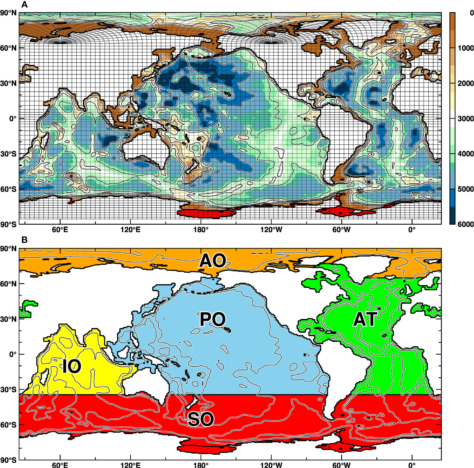
Figure 1 Model bathymetry and the defined five oceans. Ice-shelf grids are shown in red. In (A), black lines show subsampled boundaries of the model grids. (B) indicates the five oceans classified in this study: the Southern Ocean (SO, red), Atlantic Ocean (AT, green), Arctic Ocean (AO, orange), Indian Ocean (IO, yellow), and Pacific Ocean (PO, blue).

The initial condition of the model was calculated from water properties in World Ocean Atlas 2018 (Locarnini et al., 2018; Zweng et al., 2019) with zero ocean velocity field, and from this state, the model was spun up for 1500 years using present-day surface boundary conditions. The surface boundary conditions are wind stresses for the momentum equations, wind speed for calculating the surface heat fluxes, 2-m temperature, 2-m specific humidity, downward longwave radiation, downward shortwave radiation, surface freshwater flux, and sea surface pressure. We calculated them from a climatology dataset, OMIP3rd forcing (Röske, 2006), with a bulk formula (Kara et al., 2000). In this study, surface salinity was restored to the observed values over the global ocean with a 2.5-day damping timescale for the 2-m sea-surface layer to obtain realistic ocean and sea-ice states in a low-resolution model. After the 1500-year spin-up integration, we conducted virtual passive tracer experiments for 1000 years. Since Antarctic ice shelves continuously release freshwater (due to melting by the ocean), contributing to sea-level rise, we adjusted the global mean sea-level to zero using a 30-day restoring timescale. This global sea-level adjustment does not distort the local ocean dynamics.

We divided the global ocean into five regions of the Southern Ocean (SO), Atlantic Ocean (AT), Arctic Ocean (AO), Indian Ocean (IO), and Pacific Ocean (Figure 1B). Five independent tracers were placed uniformly throughout the water column with the concentration of 1.0 in the defined regions, and we examined how each tracer spreads and the timescale. These tracers were experienced with the same advection-diffusion equation as the temperature and salinity in the model. We assumed that the passive tracers have no interaction with sea ice and atmosphere. This unique experiment with the independent idealized tracers provides a comprehensive coverage across the global ocean, allowing us to grasp a holistic understanding of the timescale and pathway across the global basins. Such a wide-ranging approach promises unparalleled insights into the interconnected behavior of the global oceans.

2.2 Calculation of basin-scale tracer replacement timescales

Table 1 shows the surface area and volume of the five defined oceans in this study. The volume ratio represents the tracer ratio that each ocean grid cell should have after all tracers are completely mixed. Hereinafter, we refer to this ratio as the reference concentration (R_c). Each passive tracer is advected and diffused from its initial location to other oceans along with the modeled ocean fields. In this study, the sum of the five independent tracers’ concentration is called the total tracer, and the ratio of each tracer to the total tracer is examined in detail in the five oceans and each grid cell. Generally, the e-folding time scale is employed to measure the timescale for a transition process. In this study, considering the reference concentration and percentage of the targeted tracer relative to the total tracer, we introduced the following equation to determine the threshold value of the tracer, and we estimated tracer replacement timescale of each ocean, which is the elapsed time when the tracer reaches this threshold value (Th).

TABLE 1

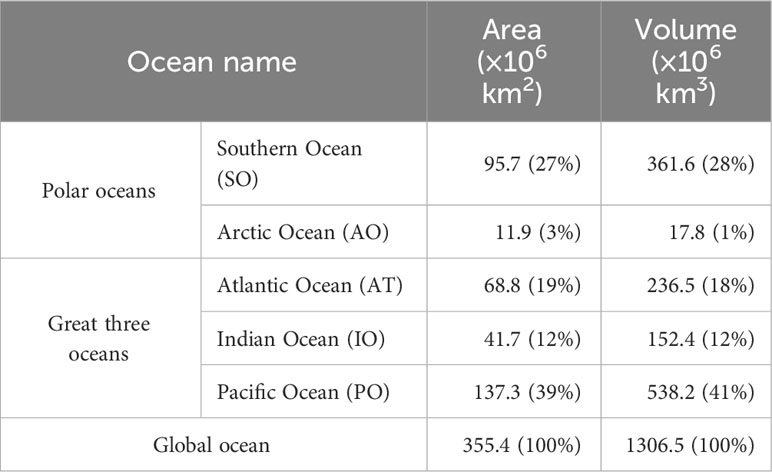
Table 1 Areas and volume of the defined five oceans.

$$\mathit{\text{Th}}={\mathit{\text{R}}}_{\mathit{\text{c}}}+(\mathbf{1}-{\mathit{\text{R}}}_{\mathit{\text{c}}})exp(-1)$$

The threshold values for SO, AO, AT, IO, and PO are 54.3%, 37.6%, 48.2%, 44.2%, and 62.8%, respectively. In other words, the tracer replacement timescale defined in this study corresponds to an e-folding timescale for each tracer asymptotically approaching the reference concentration.

3 Results

In this section, we first present quasi-steady ocean circulations reproduced in the model, and then describe the tracer replacement timescale and pathways of the passive tracers. Figure 2 displays distributions of barotropic stream function and sea-surface temperature (Figure 2A) and global meridional overturning circulation (Figure 2B). We calculated the climatological fields averaged over the last 100 years. Despite the typical issues associated with coarse resolution ocean models, such as overestimation of the Antarctic Circumpolar Current’s transport through the Drake Passage and overshooting of the Kuroshio Current, the model can roughly reproduce basin-scale ocean circulations, including the subtropical and subpolar circulations (Indian Ocean Gyre, North/South Pacific Gyre, North/South Atlantic Gyre, Weddell Gyre, and Ross Gyre). Regarding the meridional stream function, both the upper and the lower cells are reasonably represented. The Atlantic meridional overturning circulation (AMOC) and Pacific meridional overturning circulation (PMOC) are shown in Supplementary Figure 1. Although the surface boundary conditions differ, the overall picture of the meridional circulations reproduced in this model is similar to those in MIROC (Tatebe et al., 2019) and is also similar to the multi-model mean shown in the global ocean model intercomparison study (Tsujino et al., 2020). Note that the magnitude of the Antarctic Bottom Water (AABW) cell in our model (approximately 18 Sv) aligns well with previous studies’ estimate of the AABW formation/transport rate that have converged around 20 Sv (Jacobs, 2004). Similarly, the AMOC magnitude of approximately 21 Sv in this model (Figure 2B, Supplementary Figure 1) is in reasonable agreement with the observation-based estimate of 17.6 Sv (Lumpkin and Speer, 2007), considering the uncertainties that can occur in both the model and observation. These results give us some confidence in the model’s representation of ocean circulations to justify proceeding with passive tracer experiments using the ocean circulations in this model.

FIGURE 2

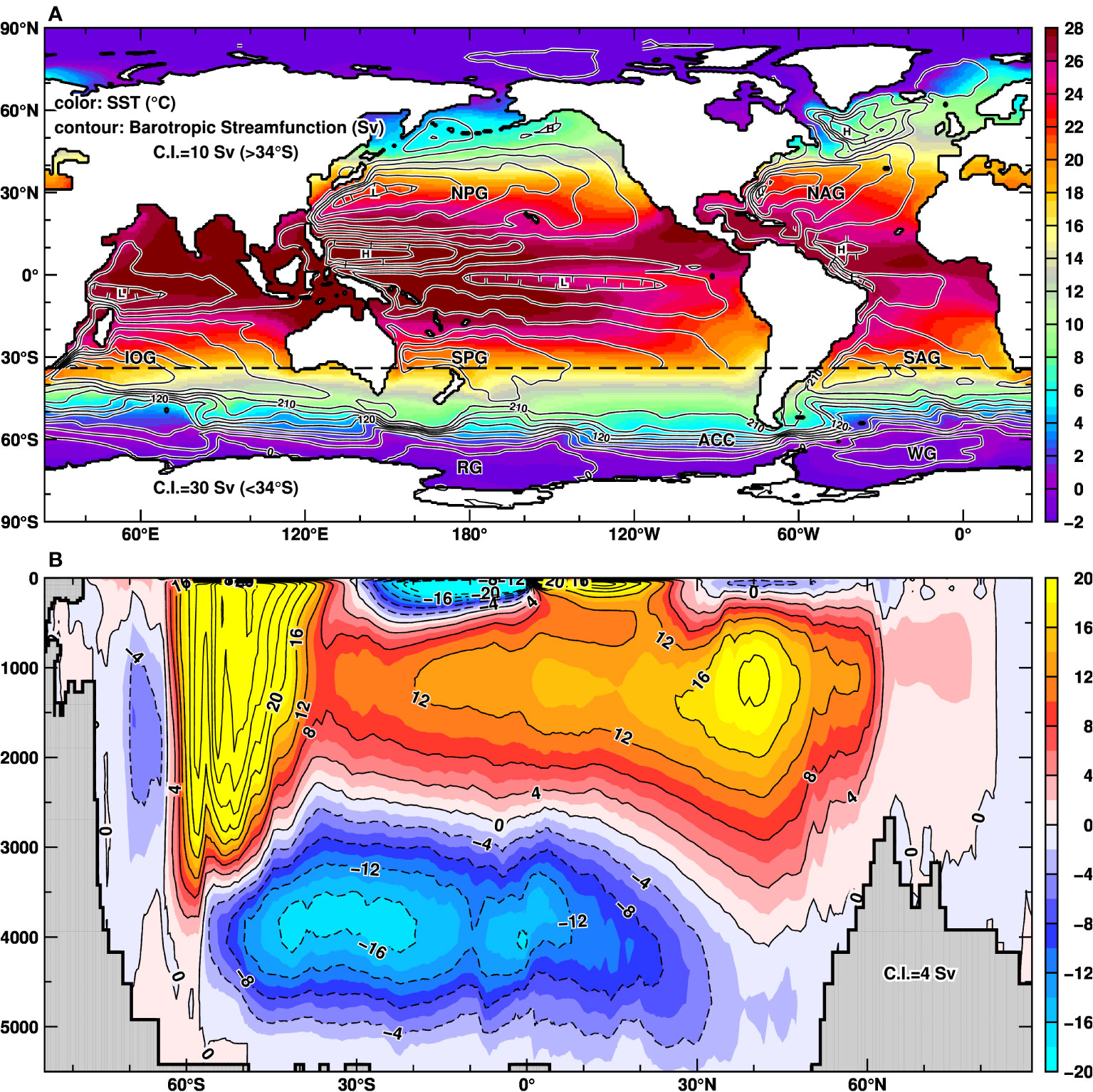
Figure 2 Stream functions of ocean circulations in the model (A: vertically-integrated transport and B: global meridional overturning circulation). Color in (A) shows annual-mean sea surface temperature. Major ocean gyre names are indicated: North/South Atlantic Gyre (NAG/SAG), North/South Pacific Gyre (NPG/SPG), Indian Ocean Gyre (IOG), Antarctic Circumpolar Current (ACC), Weddell Gyre (WG), and Ross Gyre (RG). The plots are based on averages for the last 100 years.

3.1 Basin-scale tracer replacement timescales

Time evolutions of the five passive tracers’ concentrations in each ocean basin are shown in Figure 3. The estimated tracer replacement timescale is plotted as a circle when the concentration of the local tracer falls below the threshold value, Th. The squares indicate the third-fold e-folding timescale at which the concentration of the tracer falls below the more severe value, Rc+(1−Rc) exp(−3). The tracer replacement timescales for the Southern Ocean and the Arctic Ocean are estimated to be 114 and 109 years, respectively. The Atlantic, Indian, and Pacific Oceans are estimated to be 217, 163, and 338 years, respectively. It is found that the tracer replacement timescales in the polar oceans are shorter than those in the three oceans. Similar calculations were also performed targeting only the surface layer (0−500 m) and the intermediate to deep layers (below 1000 m). Figures corresponding to these calculations can be found in Supplementary Figures 2, 3, respectively. Table 2 summarizes the estimated tracer replacement timescales for the entire water column, the surface layer (0−500 m), and the intermediate to deep layers (below 1000 m). In all basins, the timescale for the surface layer is short and the timescale for the intermediate-deep layer is long. This reflects the dominant influence of wind-driven horizontal circulation in the surface layer (Figure 2A), which is responsible for the faster response, as opposed to the more gradual influence of the Meridional Overturning Circulation (MOC) in the intermediate to deep layers (Figure 2B, Supplementary Figure 1).

FIGURE 3

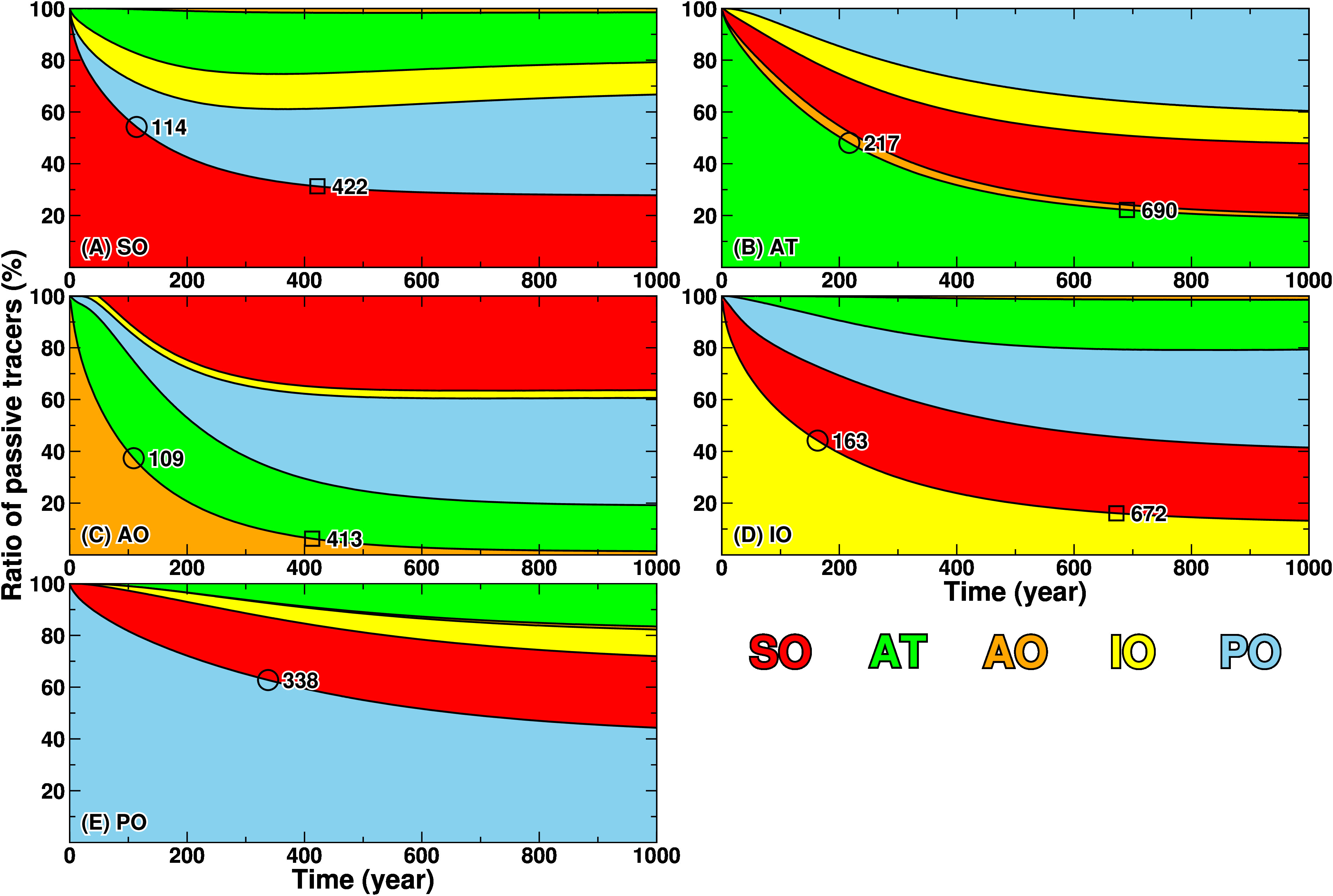
Figure 3 Time evolution of the ratio of the five tracers (A: SO, B: AT, C: AO, D: IO, and E: PO) for 1000 years. See Figure 1B for the colors of the source regions.

TABLE 2

Table 2 Estimated basin-scale tracer replacement timescales (in years).

In Section 3.2, we begin by illustrating the spreading pathways of the passive tracers originating from the Southern Ocean and the Atlantic Ocean. The reason is that the Southern Ocean is the unique ocean directly connected to the Atlantic, Indian, and Pacific Oceans, and the behavior of the local tracer (SO) is helpful for understanding the pathways of the other tracers. The Atlantic Ocean connects the two polar oceans, and thus understanding the pathway of the AT tracer also contributes to a better understanding of global tracers’ distribution and pathways of the other tracers. The other tracers in the Arctic Ocean, Indian Ocean, and Pacific Ocean are described in Section 3.3.

3.2 Southern Ocean (SO) and Atlantic Ocean (AT)

We describe the distributions and pathways of the five passive tracers from the source regions (Figures 4–8) and the time evolution of the tracers in the five basins (Figure 3). Figures 4–8 show the horizontal (surface: 0−500 m average and mid/deep depth: 2500−3500 m/3500−4500 m average) and zonal-mean distributions of the target tracers at the tracer replacement timescales. In these figures, the distributions were normalized with the reference concentrations to account for differences in the tracers’ total amount (Table 1), allowing us to illustrate the distributions in a single framework. In the normalized concentration, a value of 1.0 or greater outside of the source region serves as an indicator that the target tracer is efficiently being advected and diffused, representing a “spreading” phenomenon of the tracer from its source to other regions. Conversely, a value smaller than 1.0 in the source region suggests that the target tracer is being replaced or diluted by the other tracers, indicating a “replacement/dilution” process. By examining these distributions in detail, we can obtain valuable insights into the pathways of the regional ocean tracers and the tracer replacement between the ocean basins. Animations of the horizontal distribution up to 300 years are available in the Supplementary Material (Supplementary Movies 1−5), and they are very helpful for understanding the following descriptions of the spreading pathways of the passive tracers.

FIGURE 4

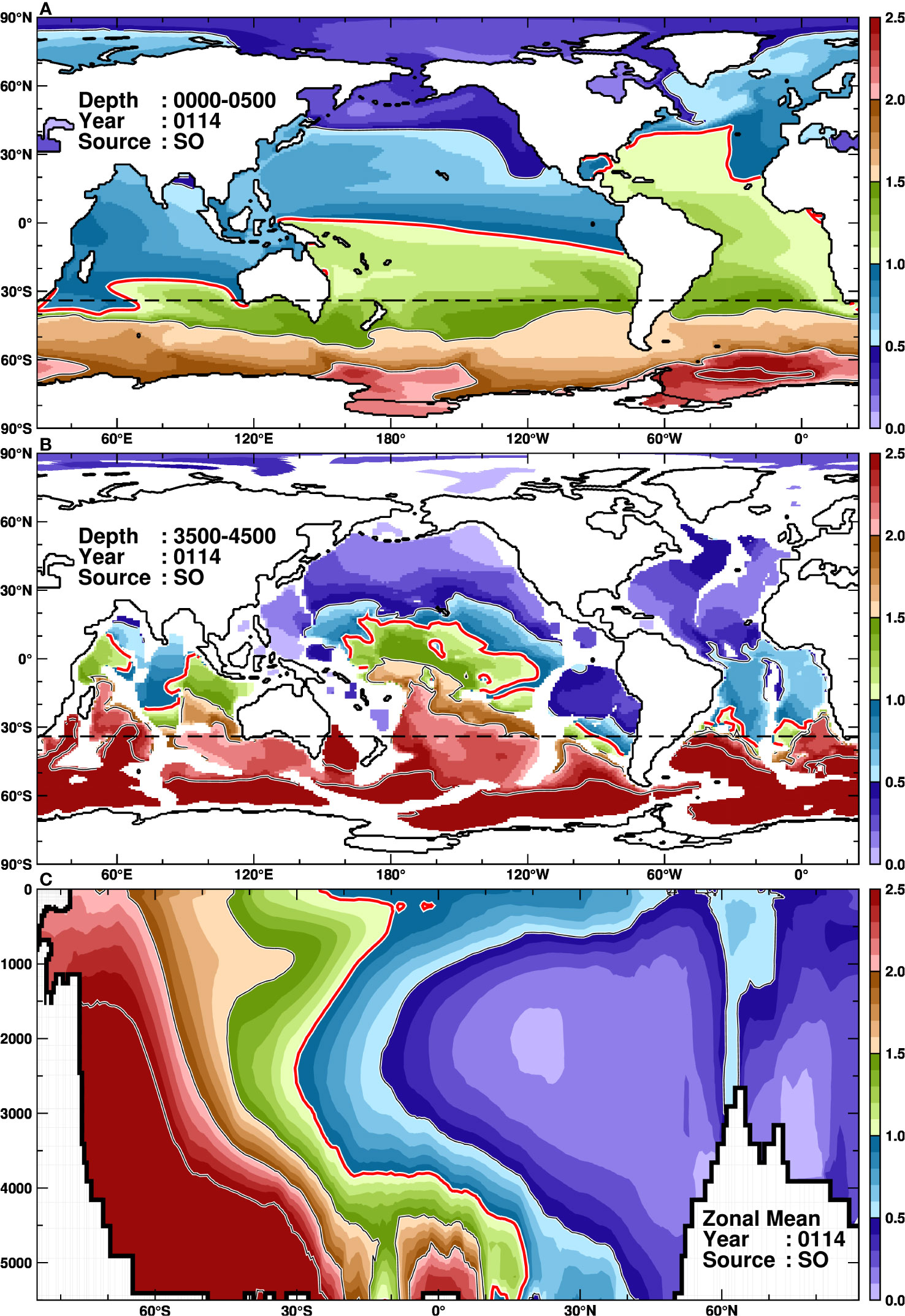
Figure 4 Spatial distribution of the normalized concentration for the SO tracer at the tracer replacement timescale (114 years), averaged across the surface (A, 0−500 m) and deep (B, 3500−4500 m) layers, respectively. (C) presents the zonal mean of the normalized concentration. The red contours represent a value of 1.0.

FIGURE 5

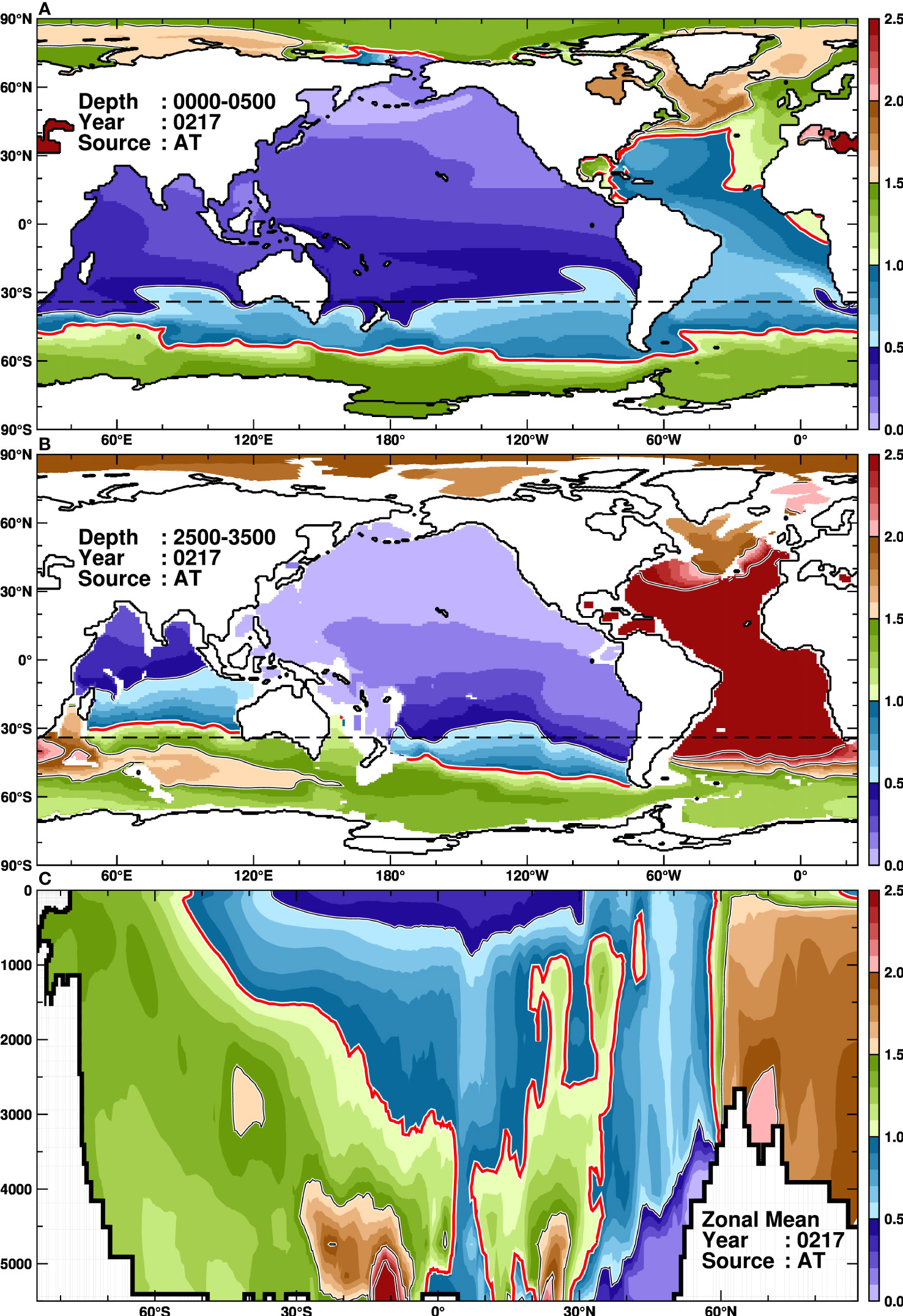
Figure 5 As in Figure 4 (A, C), but for the AT tracer at 217 years. (B) displays the spatial distribution at an intermediate depth, averaging between 2500 and 3500 m.

FIGURE 6

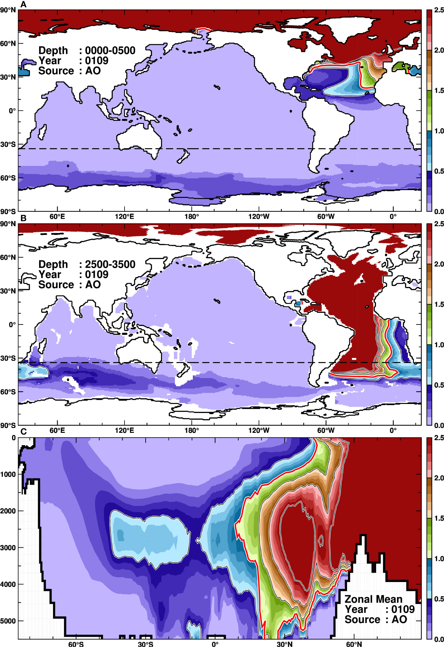
Figure 6 As in Figure 5, but for the AO tracer at 109 years.

FIGURE 7

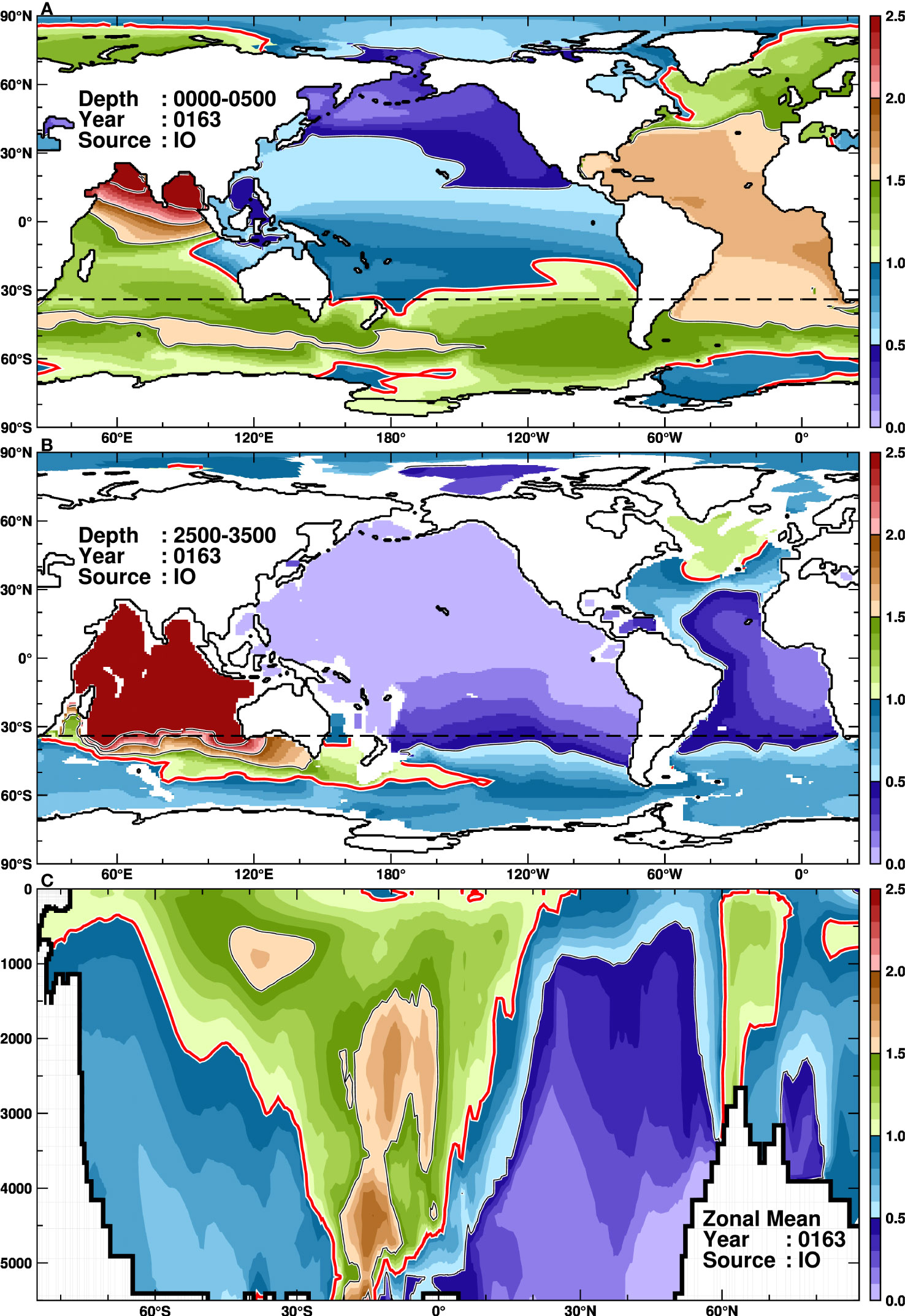
Figure 7 As in Figure 5, but for the IO tracer at 163 years.

FIGURE 8

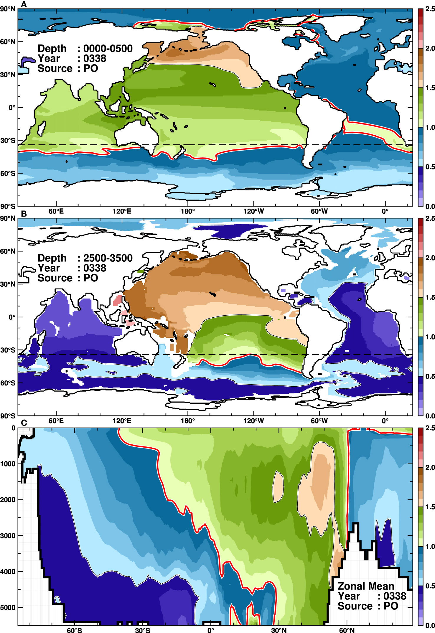
Figure 8 As in Figure 5, but for the PO tracer at 338 years.

The SO tracer is efficiently transported northward in both the surface and deep layers (Figure 4, Supplementary Movie 1). Note that we configured the color scale in the figures to highlight values with increments of 0.5, and the value of 1.0 is emphasized with thick red contours. Examining the surface distribution illustrates that the SO tracer is efficiently transported northward in the Atlantic Ocean (Figure 4A). The 1.0 contour reaches up to around 50°N in the Atlantic Ocean, while in the Indian and Pacific Oceans, it only extends to around 30°N and near the equator, respectively. In the Southern Ocean, high concentration zones of the SO tracer are found near the Weddell and Ross Gyres, indicating areas where the local tracer tends to remain in the source region. Next, looking at the deep layers, the 1.0 contour extends to around 30°N beyond the Northern Hemisphere across the equator in the Indian and Pacific Oceans, while in the Atlantic Ocean it only reaches up to around 20°S. This deep distribution of the SO tracer corresponds to the spreading of AABW along the ocean flow of the lower cell of the global MOC (Figure 2B). The differences of the SO tracer in the deep layer among the basins can be attributed to the southward flow in the lower layer of the AMOC (Supplementary Figure 1), which suppresses the northward expansion in the Atlantic Ocean, and the northward flow in the lower layer of the PMOC, which efficiently transports the tracer northward in the deep Indian and Pacific Oceans. The vertical distribution of the normalized concentration reveals that the 1.0 contour extends to around 20°N beyond the equator in deep layers but only reaches up to around 10°S in the surface layer (Figure 4C). However, focusing on the boundary of the 0.5 contours, the surface layer extends up to approximately 60°N, while it only reaches up to around 40°N in the deep layer. This indicates that the surface route very efficiently transports the SO tracer toward the North Atlantic and Arctic Oceans, although the total volume is smaller than that in the deep layer.

The time evolution of the passive tracers in the Southern Ocean demonstrates that each tracer asymptotically approaches the reference concentration after the three-fold tracer replacement timescale, 422 years (Figure 3A). The Atlantic Ocean (AT) and Indian Ocean (IO) tracers reach constant values after approximately 250 years, while the Pacific Ocean (PO) exhibits a slower response, reflecting the longest tracer replacement timescale.

Next, we examine the behavior of the AT tracer (Figure 5, Supplementary Movie 2). The surface AT tracer becomes below the reference concentration after the tracer replacement timescale (Figure 5A), indicating a rapid and effective replacement of the surface waters with the surrounding oceans (Table 2). The AT tracer widely spreads to the Arctic Ocean and the Southern Ocean, where the normalized concentration of the AT tracer is over 1.0. Looking at the middle layer (Figure 5B), although the local AT tracer remains in the source region, the AT tracer spreads to both polar oceans as in the surface layer. In both the Arctic and Southern Oceans, the concentrations in the middle layer are higher than in the surface layer, indicating that the middle layer is an efficient pathway of the AT tracer to the polar regions (Figure 5C). In the surface and middle layers of the Indian and Pacific Oceans, there is no substantial amount of the AT tracer. The pathway of the AT tracer in the middle layer over the Southern Ocean shows that the tracer moves eastward from the south of Africa along the southern part of the South Atlantic Gyre (i.e., the northern part of the eastward-flowing ACC), forming a tongue-like shape, and it is gradually upwelled to the surface layer in the Southern Ocean. Looking at Figure 3B, each tracer in the Atlantic Ocean is expected to asymptotically approach the reference concentration after the third-fold e-folding tracer replacement timescale (690 years). The SO, AT, and IO tracers, which are closer in geographical distance, approach the reference concentrations, whereas the PO tracer responds most slowly.

3.3 Arctic Ocean (AO), Indian Ocean (IO), and Pacific Ocean (PO)

The Arctic Ocean accounts for 3% of the total ocean surface area but only for about 1% of the volume (Table 1). Therefore, the Arctic Ocean is strongly influenced by the surrounding oceans, especially the adjacent Atlantic Ocean. A high concentration zone of the AO tracer in the surface layer extends southward along the Canary Current (the eastern side of the North Atlantic Gyre), but the contour of the normalized concentration of 1.0 reaches only 20°N (Figure 6A). The most intriguing behavior of the AO tracer is its transport in the middle layer (Figure 6B). There are high concentration zones in the middle layer and the edge of the 1.0 contour reach 45°S in the Atlantic Sector of the Southern Ocean. This result indicates that the middle layer in the Atlantic Ocean acts as a very efficient conduit of the AO tracer to the Southern Hemisphere. The animation of the AO tracer clearly shows its southward movement along the western coast of the Atlantic Ocean (Supplemental Movie 3). At the tracer replacement timescale (109 years), the AO tracer does not reach the Indian or Pacific Oceans in sufficient amounts. Figure 6C also illustrates that the AO tracer reaches the Southern Ocean in the mid-depth layer (i.e., along the southward component of AMOC) and upwells to the surface layer over the Southern Ocean. After 109 years, the AO tracer spreads to the Indian and Pacific Oceans in a similar pathway of the SO tracer (Figure 4). Focusing on the tracer evolution in the Arctic Ocean (Figure 3C), the contribution of the adjacent AT tracer first increases rapidly, then the contributions from the SO and IO tracers level off after a few hundred years. As in other regions, the contribution of the PO tracer takes the longest time to become constant.

The surface distribution of the IO tracer at the tracer replacement timescale (163 years) shows that the regional tracer in the southern half of the Indian Ocean is mostly transported into the Atlantic Ocean or the Southern Ocean, while the tracer in the northern half is relatively stagnant (Figure 7A). It should be noted that the model may underestimate tracer transport along the surface route due to insufficient model resolution, as it fails to capture the westward-moving eddies responsible for effective tracer transport in reality (Biastoch et al., 2008; Tsugawa and Hasumi, 2010; Schmidt et al., 2021). In this model, the pathway of the IO tracer to the Atlantic Ocean is first southward along the east coast of African continent by the Agulhas Current, and after passing through the southern tip of Africa, it veers northward into the Atlantic Ocean, by the Benguela Current (the eastern part of the South Atlantic Gyre). The IO tracer entering the Atlantic Ocean reaches the North Atlantic and Arctic Ocean rapidly, as described for the SO tracer. In fact, the 1.0 contour of the normalized concentration reaches around 85°N within the tracer replacement timescale. On the other hand, the IO tracer flowing into the Southern Ocean is advected eastward by the ACC and spread over the Southern Ocean. A part of the IO tracer approaching the Drake Passage is swept northward along the western coast of South America by the Peru Current (eastern part of the South Pacific Gyre) and enters the Pacific Ocean. The rest of the tracer passing through the Drake Passage flows into the Atlantic Ocean or circulates within the Southern Ocean along the ACC. In the middle layer, there is no route to the Atlantic Ocean through the southern tip of Africa, but only the Southern Ocean route via the ACC is evident. Interestingly, a high concentration zone in the middle layer is found in the south of Greenland, which is isolated from the main middle-depth route, and it signifies that the surface tracer in the fast pathway undergoes deep water formation and vertical advection to the middle layer. The high concentration along the ACC is found in the range from the surface to 3000 m (Figures 7B, C). Within the tracer replacement timescale, the IO tracer does not reach the central or deep parts of the Pacific Ocean. The time evolution of the five passive tracers in the Indian Ocean shows that the SO, AT, and PO tracers enter at similar timescales. This is because the Indian Ocean is adjacent to the Pacific Ocean, and enough PO tracers are transported to the Indian Ocean via Indonesian throughflows.

The Pacific Ocean exhibits a longer tracer replacement timescale (338 years) than the other four oceans (109−217 years). The surface distribution of the PO tracer reveals higher concentrations in the surface and middle layers of the North Pacific (northern part of the source region), where the tracer remains in the source region (Figure 8, Supplementary Movie 5). Within the surface layer (up to 200 m deep), a part of the PO tracer passes through the Bering Strait and spreads to the Arctic Ocean (Figures 8A, C). The surface PO tracer is efficiently transported southwestward to the Indian Ocean via the Indonesian throughflows, with normalized concentrations exceeding 1.0 throughout the Indian Ocean. A portion of the PO tracer entering the Indian Ocean flows into the South Atlantic Ocean via the southern tip of Africa in a similar pathway of the IO tracer (Figure 7A). Indeed, the 1.0 contours of the normalized concentration are identified in the Atlantic Ocean with a tongue-like feature extending from the southern tip of Africa to the northwest. The PO tracer rapidly spreads over the Atlantic Ocean in the surface layer, reaching the North Atlantic and the Arctic Ocean. Looking south, the PO tracer reaches the northern part of the ACC region around 60°S but rarely extends to the Antarctic coastal region. In the middle layer, there is no direct transport of the PO tracer to the Indian Ocean, Atlantic Ocean, or Antarctic coastal regions (Figure 8B). In the North Atlantic Ocean, a relatively high concentration zone (above 0.5 in the normalized concentration) is found, but this is due to transport from the surface layer through the Indian and Atlantic Oceans via deep water formation in the North Atlantic Ocean. In the deeper layers, the PO tracer is diluted mainly by the SO tracer (Figure 4C), reflecting the PMOC flow field (Figure 2, Supplementary Figure 1). The temporal evolution of the five tracers in the Pacific Ocean shows a quick inflow of the SO tracer, followed by the inflow of the AT and IO tracers of the Indian Ocean, slowly approaching a steady state. Note that the three-fold timescale for the PO tracer cannot be estimated in 1000 years of our numerical integration.

3.4 Decay timescales in Antarctic coastal margins

A unique feature of our newly developed OGCM is its ability to represent ocean circulation in the Antarctic ice-shelf cavities, thereby allowing us to examine not just basin-scale dynamics but also more localized features. In this context, we focus on the FRIS/RIS and the Antarctic coastal regions, a setting that highlights the model’s capabilities and offers insights into regional timescales unattainable by traditional global models without an ice-shelf component. We analyzed the decay timescales of the SO tracer in a similar manner of estimating the tracer replacement timescale. Here, we use the term “decay timescale” to capture the dilution process of the SO tracer in the ice shelf cavities and Antarctic coastal regions, because these regions are part of the Southern Ocean (SO). This analysis provides insight into the artificial northern boundary in regional circumpolar Southern Ocean models (e.g., Kusahara et al., 2023), suggesting a measure of the applicable timescale for the regional models.

The decay timescales of the SO tracer in the FRIS and RIS cavities were estimated to be 156 years for the FRIS and 140 years for the RIS, respectively (Figure 9A). These timescales for the ice-shelf cavities are longer than the tracer replacement timescale of the entire Southern Ocean (114 years), indicating that the FRIS and RIS are less influenced by water masses from outside the Southern Ocean. In both ice shelves, the tracers’ ratio of the inflowing water’s origins is similar after the decay time scale, but in the first 50 years, the composition differs significantly between the two: in the FRIS, Atlantic water predominates in the initial stage, while in the RIS, the water from the Indian Ocean dominates first followed by the Atlantic-origin water (Figure 9).

FIGURE 9

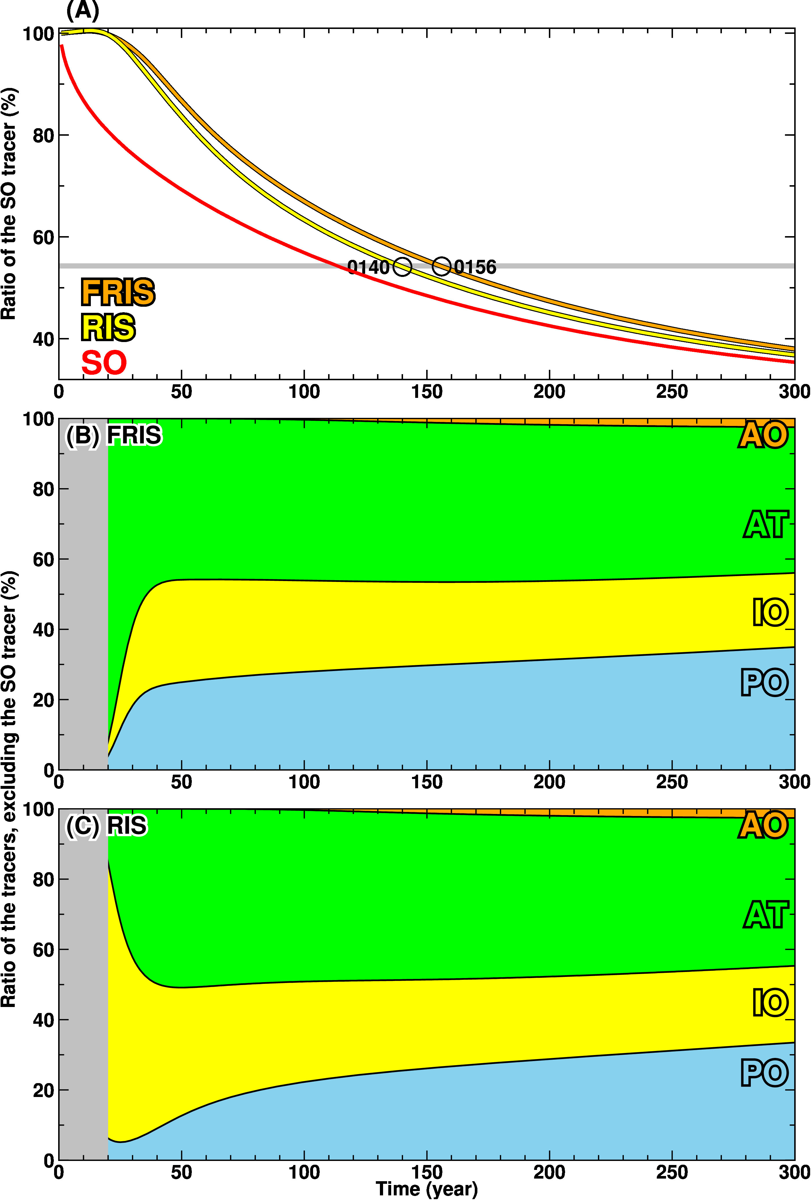
Figure 9 Decay timescales of the FRIS and RIS cavities (A) and time evolutions of the ratio of the tracers excluding the SO tracer in the cavities (B: FRIS and C: RIS). The gray line in (A) shows the threshold value of the SO tracer. The first 20 years are masked out with gray because the SO tracer is predominant for the period.

Next, we calculated the decay timescale of the SO tracer in a longitude-depth dimensions Figure 10A), dividing the Antarctic coastal margin into 20° longitudinal bands (see red, green, and blue areas in Figure 10B). It is evident that the decay timescale varies substantially with longitude and depth: it is relatively short, less than 120 years, from the surface to 400 m, and it exceeds 160 years at depths deeper than 1000 m. The shortest timescale of less than 110 years is found at 40−140°E and 160−60°W in the surface layer, and in particular, the shortest timescale of less than 100 years is found at 120−140°E. These regions with short decay timescales are located on the eastern side of the subpolar gyres of the Weddell Gyre, Kelgueren Gyre, and Ross Gyre, where water masses from the low-latitude ocean across the ACC approach the Antarctic coast. In contrast, in the western part of the gyres, the decay timescale becomes longer. The FRIS and RIS mentioned earlier (Figure 9A) are situated in this area.

FIGURE 10

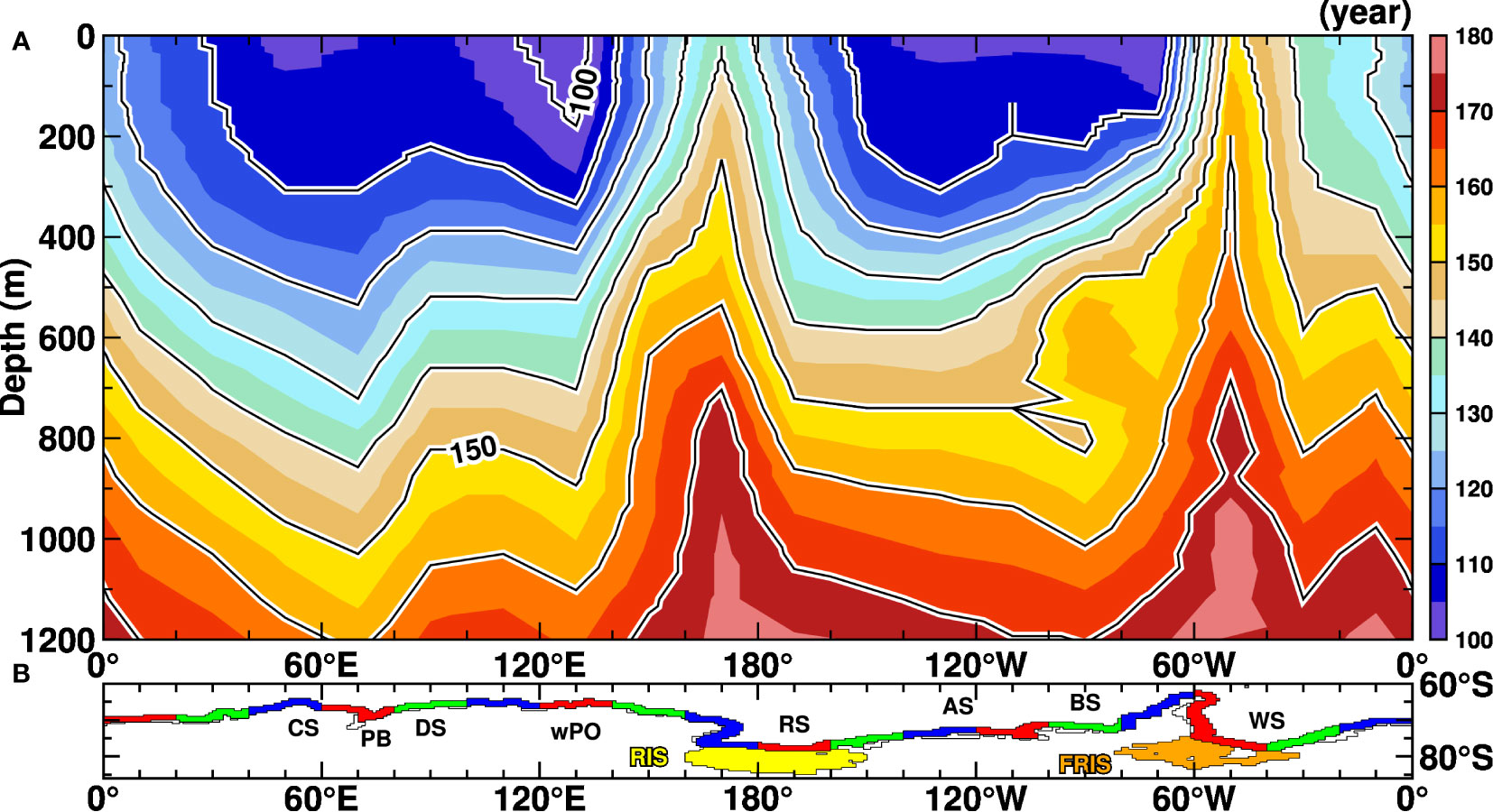
Figure 10 Decay timescales of the SO tracer along Antarctic coastal regions (A). (B) shows the defined Antarctic coastal regions to calculate the regional decay timescales. The major geographic locations within the Southern Ocean are indicated: Cosmonauts Sea (CS), Prydz Bay (PB), Davis Sea (DS), western Pacific Ocean (wPO), Ross Sea (RS), Amundsen Sea (AS), Bellingshausen Sea (BS), and the Weddell Sea (WS).

4 Summary and discussion

In this study, we utilized a one-degree global OGCM to explore the tracer replacement timescales of the two polar oceans (Southern Ocean and Arctic Ocean) and the three oceans (Atlantic, Indian, and Pacific Oceans). Our comprehensive series of passive tracer experiments reveal that tracer replacement timescales in the polar oceans are markedly shorter than those in the three oceans (Figure 3, Table 2). Here, we briefly outline the pathways of the passive tracer from each ocean basin. The Southern Ocean tracer has two major pathways to reach the Northern Hemisphere: the rapid surface route toward the Atlantic and Arctic Oceans and the deep routes toward the Indian and Pacific Oceans (Figures 2, 4) along the pathways of Antarctic Bottom Water (Orsi et al., 1999; Kusahara et al., 2017). The Atlantic Ocean tracer is widely transported to both the Arctic and Southern Oceans (Figure 5). The concentration of the Atlantic Ocean tracer in the middle layers of the polar regions is higher than in the surface layers, indicating an efficient pathway. A key feature of the Arctic Ocean tracer behavior is its efficient southward transportation via the middle layer of the Atlantic Ocean to the Southern Ocean (Figure 6). This finding underscores the crucial role of the mid-depth AMOC in global ocean circulation, linking the two hemispheres (Figure 2, Supplementary Figure 1). The Indian Ocean tracers clearly delineate two surface pathways: one extending to the Atlantic Ocean via the southern tip of Africa, and the other spreading to the Southern Ocean along the eastward-flowing ACC. In the middle layer, the tracer spreads to the Southern Ocean along the ACC (Figure 7). The Pacific Ocean tracer is characterized by a notably longer tracer replacement timescale and exhibits unique pathways. Most of the tracer remains in the North Pacific, reflecting the longest tracer replacement timescale. A portion of the surface tracers are efficiently transported to the Indian Ocean via the Indonesia throughflow (Figure 8) and then follow a similar pathway as the Indian Ocean tracer (Figure 7).

Since the global OGCM used in this study explicitly represents ice-shelf cavities, we were able to determine the decay timescales of the Southern Ocean tracer in the FRIS and RIS cavities (Figure 9) as well as the Antarctic coastal regions (Figure 10). The decay timescale for the Antarctic coastal regions, including the ice shelves, is longer than the tracer replacement timescale for the entire Southern Ocean, meaning that the influence from outside the Southern Ocean takes longer to affect the coastal and the ice-shelf regions. We observed a pronounced longitudinal-depth variation in the decay timescales along the Antarctic coastal margin. Shorter timescales were found in the surface layer and the eastern sectors of subpolar gyres, whereas longer timescales were found in the deeper layers and western portions of the gyres. The west-east contrast of the transport timescale on the coastal regions can be explained by the ocean circulation patterns (Figure 2A).

Although the tracer replacement timescales estimated in this study (Figure 2) are not directly comparable due to the specific design of our passive tracer experiments, which were aimed solely to diagnose tracer replacement timescales and pathways within our model, we find it enlightening to draw parallels with the timescales of deep ocean circulation derived from Carbon-14 (14C) in the existing literature. Particularly, Stuiver et al. (1983), using abyssal 14C distribution, calculated the replacement times of the three great oceans, identifying the Atlantic, Indian, and Pacific Oceans to have replacement times of 275, 250, and 510 years, respectively. The study proposed that global deep-sea waters are replaced on a timescale of about 500 years. Similarly, Matsumoto (2007) considered the older ages of ¹⁴C in the surface layer and the formation of deep water in both polar regions and calculated ¹⁴C circulation ages, demonstrating that the ages could range into several hundreds of years (288 years for the Atlantic Ocean, 716 years for the Indian Ocean, 889 years for the Pacific Ocean, and 295 years for the Southern Ocean). The timescales estimated in all these studies, including this study, are in the range of several hundred years, with the Pacific Ocean consistently displaying the longest timescale in the world ocean. It’s pertinent to note that the shorter timescales estimated in our study compared to those from ¹⁴C studies may be partially attributed to our incorporation of surface-to-subsurface tracers whose rapid exchange shortens the timescales (Table 2, Supplementary Figures 2, 3).

The estimation of tracer replacement timescales for global ocean basins, as conducted in this study, requires long-term integrations of approximately a thousand years. The inclusion of additional tracers further increases computational costs, and thus making use of one-degree global OGCM is an appropriate option for such a long-term integration at the current stage. However, needless to say, low-resolution ocean models cannot adequately capture ocean circulation and transport caused by unresolved mesoscale eddies and small-scale bathymetry. Therefore, numerical experiments with higher-resolution models (e.g., 0.25° and 0.1°) may yield different timescales due to improved representations of the ocean fields. Considering these uncertainties, this study only focused on relatively large-scale oceans that can be considered less susceptible to small-scale phenomena. The ocean circulation field reproduced in this study is similar to the ensemble mean of one-degree horizontal resolution ocean models (Tsujino et al., 2020), and the results of the passive tracer experiments performed in this study are also expected to behave as the ensemble mean among the models if they have done the same tracer experiments. However, it should be noted that the timescales estimated in this study are influenced by representation of the meridional overturning circulation, and thus the timescales may differ between different models as well as how the vertical diffusion coefficient is given (Kawasaki et al., 2021; Kawasaki et al., 2022). Indeed, for a more precise assessment of the variance in tracer replacement timescales among different models, additional analogous tracer experiments should be conducted for each model. Timescales can also be estimated by using Lagrangian particles in ocean models (Matsumura and Ohshima, 2015; van Sebille et al., 2018) and analyzing them. Kawasaki et al. (2022) have successfully calculated the timescale and pathway of deep water circulation in the North Pacific Ocean by analyzing a large volume of Lagrangian particles using the modeled ocean fields. If this methodology could be applied to the output fields of various models, it could offer a valuable way to estimate timescales across models without necessitating additional tracer experiments.

Although our numerical experiments were conducted under present-day climate conditions, it is conceivable that tracer replacement timescales could be largely changed in different climate conditions, such as in glacial-interglacial cycles or projected future warming scenarios. Large global sea-level change due to climate shifts or plate tectonics could lead to the opening or closing of some key straits between ocean basins, e.g., the Panama Strait, the Bering Strait, and the Drake Passage. In such instances, the formation or loss of water exchange pathways between the different ocean basins could significantly alter the tracer replacement timescales. While the passive tracer experiments in this study are idealized, they serve as a fundamental metric to improve our understanding of global ocean dynamics in a specified climate condition. By determining tracer replacement timescales and pathways through the passive tracer experiments, we can gain a more comprehensive understanding of global oceanic material/carbon/biochemical cycles and the associated ecosystems.

Data availability statement

The raw data supporting the conclusions of this article will be made available by the authors, without undue reservation.

Author contributions

KK: Conceptualization, Formal Analysis, Funding acquisition, Investigation, Methodology, Project administration, Visualization, Writing – original draft, Writing – review & editing. HT: Supervision, Writing – review & editing.

Funding

The author(s) declare financial support was received for the research, authorship, and/or publication of this article. This work was supported by JSPS KEKENHI Grants (JP19K12301, JP21H04918, JP22H05003, and JP23H05411). KK was supported by MEXT-Program for the advanced studies of climate change projection (SENTAN) Grant Number JPMXD0722681344 and the Grant for Joint Research Program of the Institute of Low Temperature Science, Hokkaido University (23G021).

Acknowledgments

All numerical experiments with the ocean-sea ice-ice shelf model were performed on the Earth Simulator at the Japan Agency for Marine-Earth Science and Technology. We are grateful to Dr. Takao Kawasaki for useful discussion.

Conflict of interest

The authors declare that the research was conducted in the absence of any commercial or financial relationships that could be construed as a potential conflict of interest.

Publisher’s note

All claims expressed in this article are solely those of the authors and do not necessarily represent those of their affiliated organizations, or those of the publisher, the editors and the reviewers. Any product that may be evaluated in this article, or claim that may be made by its manufacturer, is not guaranteed or endorsed by the publisher.

Supplementary material

The Supplementary Material for this article can be found online at: https://www.frontiersin.org/articles/10.3389/fmars.2023.1308728/full#supplementary-material

References

Biastoch A., Böning C. W., Lutjeharms J. R. E. (2008). Agulhas leakage dynamics affects decadal variability in Atlantic overturning circulation. Nature 456, 489–492. doi: 10.1038/nature07426

PubMed Abstract | CrossRef Full Text | Google Scholar

Buckley M. W., Marshall J. (2016). Observations, inferences, and mechanisms of the Atlantic Meridional Overturning Circulation: A review. Rev. Geophys. 54, 5–63. doi: 10.1002/2015RG000493

CrossRef Full Text | Google Scholar

Cushman-Roisin B., Beckers J.-M. (2011). Introduction to Geophysical Fluid Dynamics: Physical and Numerical Aspects (Cambridge, Massachusetts: Academic Press).

Google Scholar

England M. H. (1995). Using chlorofluorocarbons to assess ocean climate models. Geophys. Res. Lett. 22, 3051–3054. doi: 10.1029/95GL02670

CrossRef Full Text | Google Scholar

Fox-Kemper B., Adcroft A., Böning C. W., Chassignet E. P., Curchitser E., Danabasoglu G., et al. (2019). Challenges and prospects in ocean circulation models. Front. Mar. Sci. 6. doi: 10.3389/fmars.2019.00065

CrossRef Full Text | Google Scholar

Gill A. E. (1982). Atmosphere-Ocean Dynamics (Cambridge, Massachusetts: Academic Press).

Google Scholar

Hajima T., Watanabe M., Yamamoto A., Tatebe H., Noguchi M. A., Abe M., et al. (2020). Development of the MIROC-ES2L Earth system model and the evaluation of biogeochemical processes and feedbacks. Geosci. Model. Dev. 13 (5), 2197–2244. doi: 10.5194/gmd-13-2197-2020

CrossRef Full Text | Google Scholar

Hasumi H. (2006) CCSR Ocean Component Model (COCO) Version 4.0. CCSR Rep. No. 25. Available at: http://ccsr.aori.u-tokyo.ac.jp/~hasumi/COCO/.

Google Scholar

Jacobs S. S. (2004). Bottom water production and its links with the thermohaline circulation. Antarct. Sci. 16, 427–437. doi: 10.1017/S095410200400224X

CrossRef Full Text | Google Scholar

Kara A. B., Rochford P. A., Hurlburt H. E. (2000). Efficient and accurate bulk parameterizations of air–sea fluxes for use in general circulation models. J. Atmos. Ocean. Technol. 17, 1421–1438. doi: 10.1175/1520-0426(2000)017<1421:EAABPO>2.0.CO;2

CrossRef Full Text | Google Scholar

Kawasaki T., Hasumi H., Tanaka Y. (2021). Role of tide-induced vertical mixing in the deep Pacific Ocean circulation. J. Oceanogr. 77, 173–184. doi: 10.1007/s10872-020-00584-0

CrossRef Full Text | Google Scholar

Kawasaki T., Matsumura Y., Hasumi H. (2022). Deep water pathways in the North Pacific Ocean revealed by Lagrangian particle tracking. Sci. Rep. 12. doi: 10.1038/s41598-022-10080-8

CrossRef Full Text | Google Scholar

Kusahara K., Hasumi H. (2013). Modeling Antarctic ice shelf responses to future climate changes and impacts on the ocean. J. Geophys. Res. Ocean. 118, 2454–2475. doi: 10.1002/jgrc.20166

CrossRef Full Text | Google Scholar

Kusahara K., Hirano D., Fujii M., D. Fraser A., Tamura T. (2021). Modeling intensive ocean-cryosphere interactions in Lützow-Holm Bay, East Antarctica. Cryosphere. 15 (4), 1697–1717. doi: 10.5194/tc-15-1697-2021

CrossRef Full Text | Google Scholar

Kusahara K., Tatebe H., Hajima T., Saito F., Kawamiya M. (2023). Antarctic sea ice holds the fate of antarctic ice-shelf basal melting in a warming climate. J. Clim. 36, 713–743. doi: 10.1175/JCLI-D-22-0079.1

CrossRef Full Text | Google Scholar

Kusahara K., Williams G. D., Tamura T., Massom R., Hasumi H. (2017). Dense shelf water spreading from Antarctic coastal polynyas to the deep Southern Ocean: A regional circumpolar model study. J. Geophys. Res. Ocean. 122, 6238–6253. doi: 10.1002/2017JC012911

CrossRef Full Text | Google Scholar

Locarnini R. A., Mishonov A. V., Baranova O. K., Boyer T. P., Zweng M. M., Garcia H. E., et al. (2018). “World Ocean Atlas 2018, Volume 1: Temperature,” in NOAA Atlas NESDIS 81. (Spring, MD: NOAA/NESDIS National Centers for Environmental Information).

Google Scholar

Lumpkin R., Speer K. (2007). Global ocean meridional overturning. J. Phys. Oceanogr. 37, 2550–2562. doi: 10.1175/JPO3130.1

CrossRef Full Text | Google Scholar

Marshall J., Speer K. (2012). Closure of the meridional overturning circulation through Southern Ocean upwelling. Nat. Geosci. 5, 171–180. doi: 10.1038/ngeo1391

CrossRef Full Text | Google Scholar

Matsumoto K. (2007). Radiocarbon-based circulation age of the world oceans. J. Geophys. Res. Ocean. 112. doi: 10.1029/2007JC004095

CrossRef Full Text | Google Scholar

Matsumura Y., Ohshima K. I. (2015). Lagrangian modelling of frazil ice in the ocean. Ann. Glaciol. 56, 373–382. doi: 10.3189/2015AoG69A657

CrossRef Full Text | Google Scholar

Nakano H., Suginohara N. (2002). Effects of bottom boundary layer parameterization on reproducing deep and bottom waters in a world ocean model. J. Phys. Ocean. 32, 1209–1227. doi: 10.1175/1520-0485(2002)032<1209:EOBBLP>2.0.CO;2

CrossRef Full Text | Google Scholar

Orr J. C., Najjar R. G., Aumont O., Bopp L., Bullister J. L., Danabasoglu G., et al. (2017). Biogeochemical protocols and diagnostics for the CMIP6 Ocean Model Intercomparison Project (OMIP). Geosci. Model. Dev. 10, 2169–2199. doi: 10.5194/gmd-10-2169-2017

CrossRef Full Text | Google Scholar

Orsi A. H., Johnson G. C., Bullister J. L. (1999). Circulation, mixing, and production of Antarctic Bottom Water. Prog. Oceanogr. 43, 55–109. doi: 10.1016/S0079-6611(99)00004-X

CrossRef Full Text | Google Scholar

Pedlosky J. (1979). Geophysical fluid dynamics. (New York City: Springer). doi: 10.4171/owr/2017/23

CrossRef Full Text | Google Scholar

Röske F. (2006). A global heat and freshwater forcing dataset for ocean models. Ocean Model. 11, 235–297. doi: 10.1016/j.ocemod.2004.12.005

CrossRef Full Text | Google Scholar

Santoso A., England M. H. (2008). Antarctic Bottom Water variability in a coupled climate model. J. Phys. Oceanogr. 38, 1870–1893. doi: 10.1175/2008JPO3741.1

CrossRef Full Text | Google Scholar

Schaffer J., Timmermann R., Erik Arndt J., Savstrup Kristensen S., Mayer C., Morlighem M., et al. (2016). A global, high-resolution data set of ice sheet topography, cavity geometry, and ocean bathymetry. Earth Syst. Sci. Data 8, 543–557. doi: 10.5194/essd-8-543-2016

CrossRef Full Text | Google Scholar

Schmidt C., Schwarzkopf F. U., Rühs S., Biastoch A. (2021). Characteristics and robustness of Agulhas leakage estimates: An inter-comparison study of Lagrangian methods. Ocean Sci. 17, 1067–1080. doi: 10.5194/os-17-1067-2021

CrossRef Full Text | Google Scholar

Stephenson D., Müller S. A., Sévellec F. (2020). Tracking water masses using passive-tracer transport in NEMO v3.4 with NEMOTAM: Application to North Atlantic Deep Water and North Atlantic Subtropical Mode Water. Geosci. Model. Dev. 13, 2031–2050. doi: 10.5194/gmd-13-2031-2020

CrossRef Full Text | Google Scholar

Stuiver M., Quay P. D., Ostlund H. G. (1983). Abyssal water carbon-14 distribution and the age of the world oceans. Sci. (80-.). 219, 849–851. doi: 10.1126/science.219.4586.849

CrossRef Full Text | Google Scholar

Suzuki T., Komuro Y., Kusahara K., Tatebe H. (2022). Transient influence of the reduction of deepwater formation on ocean heat uptake and heat budgets in the global climate system. Geophys. Res. Lett. 49. doi: 10.1029/2021GL095179

CrossRef Full Text | Google Scholar

Talley L. D. (2013). Closure of the global overturning circulation through the Indian, Pacific, and southern oceans. Oceanography 26, 80–97. doi: 10.5670/oceanog.2013.07

CrossRef Full Text | Google Scholar

Tatebe H., Ogura T., Nitta T., Komuro Y., Ogochi K., Takemura T., et al. (2019). Description and basic evaluation of simulated mean state, internal variability, and climate sensitivity in MIROC6. Geosci. Model. Dev. 12, 2727–2765. doi: 10.5194/gmd-12-2727-2019

CrossRef Full Text | Google Scholar

Tsugawa M., Hasumi H. (2010). Generation and growth mechanism of the natal pulse. J. Phys. Oceanogr. 40, 1597–1612. doi: 10.1175/2010JPO4347.1

CrossRef Full Text | Google Scholar

Tsujino H., Shogo Urakawa L., Griffies S. M., Danabasoglu G., Adcroft A. J., Amaral A. E., et al. (2020). Evaluation of global ocean-sea-ice model simulations based on the experimental protocols of the Ocean Model Intercomparison Project phase 2 (OMIP-2). Geosci. Model. Dev. 13, 3643–3708. doi: 10.5194/gmd-13-3643-2020

CrossRef Full Text | Google Scholar

Uchimoto K., Nakamura T., Mitsudera H. (2011). Tracing dense shelf water in the Sea of Okhotsk with an ocean general circulation model. Hydrol. Res. Lett. 5, 1–5. doi: 10.3178/hrl.5.1

CrossRef Full Text | Google Scholar

van Sebille E., Griffies S. M., Abernathey R., Adams T. P., Berloff P., Biastoch A., et al. (2018). Lagrangian ocean analysis: Fundamentals and practices. Ocean Model. 121, 49–75. doi: 10.1016/j.ocemod.2017.11.008

CrossRef Full Text | Google Scholar

Zhang R., Sutton R., Danabasoglu G., Kwon Y. O., Marsh R., Yeager S. G., et al. (2019). A review of the role of the atlantic meridional overturning circulation in atlantic multidecadal variability and associated climate impacts. Rev. Geophys. 57, 316–375. doi: 10.1029/2019RG000644

CrossRef Full Text | Google Scholar

Zweng M. M., Reagan J. R., Seidov D., Boyer T. P., Antonov J. I., Locarnini R. A., et al. (2019). “WORLD OCEAN ATLAS 2018 Volume 2: Salinity,” in NOAA Atlas NESDIS. (Spring, MD: NOAA/NESDIS National Centers for Environmental Information).

Google Scholar