Environmental, behavioral, and design-related factors affect accuracy and precision of beluga abundance estimates from aerial surveys

Introduction

Abundance is central to the management of wildlife populations (Williams et al., 2002; Cardinale et al., 2019) and is often derived from survey data (Seber, 1982; Buckland et al., 2001). While abundance estimates must be accurate to assess population conservation status, they also need precision in order to reliably detect significant population trends (Gerrodette, 1987; Taylor et al., 2007). The precision of abundance estimates often incorporates the variance from multiple factors (e.g., group size, densities, visibility corrections), and is also influenced by the number of groups sighted (Buckland et al., 2001). In species with highly clumped and heterogenous distributions, these sources of variation may inflate uncertainty, and even bias abundance estimates depending on survey design (Nomani et al., 2012). Adopting a systematic transect line placement, increasing survey coverage, and reducing the interval between survey years may help improve accuracy and precision of abundance estimates (Gerrodette, 1987; Holt et al., 1987; Nomani et al., 2012). Obtaining repeat estimates of abundance for a given year may also help achieve this goal, although data-driven demonstrations of the sensitivity of survey point abundance estimates (i.e., relative precision and accuracy) to the number of replicate surveys is generally lacking for marine mammals.

Systematic strip- and line-transect surveys are popular, statistically robust methods for estimating abundance of organisms, including cetaceans and ice-associated pinnipeds (Buckland et al., 2001; Williams et al., 2002; Elphick, 2008; Foster, 2012; Hammond et al., 2021). However, survey-derived abundance estimates can be biased when animals that are visible to observers are not seen (perception bias), or when they are unavailable to be counted because they are concealed by vegetation, boulders, other animals or turbid waters (availability bias) (Caughley, 1974; Marsh and Sinclair, 1989; Buckland et al., 2004; Brack et al., 2019). Corrections for perception and availability bias are multipliers of un-corrected counts, and can have a substantial effect on final abundance estimates (Marsh and Sinclair, 1989), and vary with survey design. In the case of photographic surveys, perception bias is generally estimated and minimized through repeated imagery readings (Gosselin et al., 2014; Stenson et al., 2014; Bröker et al., 2019). For visual surveys, perception bias is usually larger, and can be assessed by using two independent observation teams, and applying a mark-recapture distance-sampling procedure to the data (Burt et al., 2014). Correcting for availability bias is more challenging, and often requires an independent source of data on animal behavior and distribution (i.e., to estimate the likelihood of animals being visually available at the time of survey). In diving species, availability bias is primarily the result of animals being below the surface of the water, and can be estimated from circle-back or “racetrack” method during surveys (Hiby, 1999), or from the distribution of surface and dive times using a variety of approaches such as radio-telemetry data (Schweder et al., 1991), visual observations (Barlow et al., 1988; Laake et al., 1997; Kingsley and Gauthier, 2002; Slooten et al., 2004), or archival tag data (Pollock et al., 2006; Edwards et al., 2007; Fuentes et al., 2015; Watt et al., 2015a; Nykänen et al., 2015b, 2018; this study). The magnitude of the availability bias varies with survey design, and is expected to be less for visual than for photographic surveys, mainly given that the time window for detection is longer for an observer during a visual survey as compared to the snapshot of potentially detectable individuals offered via imagery (McLaren, 1961; Laake et al., 1997; Forcada et al., 2004; Gómez de Segura et al., 2006).

Various factors that are inherent to the species, or their environment, can affect availability bias (e.g., Langtimm et al., 2011; Thomson et al., 2012; Fuentes et al., 2015; Sucunza et al., 2018; Brown et al., 2023). In aquatic species, turbidity can limit depth at which animals can be detected, whereas bottom depth can modulate availability by influencing dive depth and duration (e.g., Slooten et al., 2004; Pollock et al., 2006). Seafloor depth effects on surface time or availability might be particularly strong in areas where feeding occurs at deeper depths (Martin and Smith, 1999; Doniol-Valcroze et al., 2011). Conversely, the influence of seafloor depth might be less when animals are travelling, resting, or socializing near the surface (e.g., Whitehead and Weilgart, 1991). The physiological condition and reproductive status of individuals can also affect availability. For instance, females accompanied by a calf may dive less than non-calving females or other age- or sex-classes (e.g., Dombroski et al., 2021; Brown et al., 2023). Diving capacity increases allometrically with size, causing differences in availability among age-classes, and between males and females in sexually dimorphic species (Schreer and Kovacs, 1997). Juveniles or animals in poor body condition may also forage at different depths or in different areas than adults or animals that are in better shape (i.e., Orgeret et al., 2019). However, while there is growing evidence for the need to account for environmental and behavioral factors when assessing availability bias, very few studies, if any, have provided the means for incorporating location-specific availability bias corrections, and most importantly, for propagating uncertainty associated with these corrections into final abundance estimates.

For cetaceans, abundance is often obtained through aerial or vessel-based surveys (Hammond et al., 2021). The propension of these species to spend a considerable proportion of their time away from the surface, make them more prone to both availability and perception biases. Abundance estimation is particularly challenging with these species, given their wide distribution range and clumped distributions. Distribution and clumping are generally driven by habitat heterogeneity, but for delphinids and some other species, also by social structure. The beluga (Delphinapterus leucas) is one such particularly challenging species to survey, given its highly social and gregarious nature (Michaud, 2005). Sex and age classes segregate spatially among habitats with widely different characteristics during summer, when calving occurs (Michaud, 2005; Loseto et al., 2006; Mosnier et al., 2010). While distribution range is relatively constrained during summer, drivers of habitat use are not fully understood (Mosnier et al., 2010; Hornby et al., 2016; Mosnier et al., 2016; Smith et al., 2017; Pirotta et al., 2018). As a result of their clumped distribution, and potentially coordinated behaviours, abundance estimates for beluga populations are often associated with low precision (i.e., CVs of 25—40%), with point estimates of abundance potentially varying almost 2-fold between consecutive survey days (Gosselin et al., 2017; Higdon and Ferguson, 2017; Lowry et al., 2019).

In the St. Lawrence Estuary (SLE), Canada, beluga abundance has been monitored since 1988 using systematic aerial surveys covering their entire summer range. While high-coverage (50%) strip-transect photographic surveys have been used consistently since then, lower coverage (10-15%) line-transect visual surveys, often repeated multiple times per year, have been conducted since 2001 (Kingsley and Hammill, 1991; Kingsley, 1993, 1996, 1999; Gosselin et al., 2001, 2007, 2014, 2017; St-Pierre et al., 2023). This exceptional dataset (11 photographic and 52 visual surveys), combined with dive data obtained at high spatial and temporal resolution from 27 individuals, offered a unique opportunity to examine methodological, environmental, and behavioral factors potentially affecting the accuracy and precision of abundance estimates from survey data. Specifically, we first examined the relative influence of survey design (photographic versus visual), seafloor depth, water turbidity and habitat used, as well as whether animals were likely in transit or foraging on availability bias estimates from photographic and visual aerial surveys. We also proposed a methodology to incorporate location-specific availability bias corrections and associated uncertainty into survey data analysis and abundance estimation to increase their accuracy. Finally, using a data set of 28 visual surveys repeated over a 16 to 29-day period depending on survey year (St-Pierre et al., 2023), we estimated the optimal number of surveys required to achieve adequate accuracy and precision of abundance estimates for species with a clumped distribution such as beluga.

Materials and methods

Survey data and methodology

Surveys to obtain abundance estimates for SLE beluga are conducted during summer (generally from mid-August to first week of September) when distribution is the most constrained (Mosnier et al., 2010). The Estuary portion of the beluga habitat (Zones 1 to 3 in Figure 1) is flown using systematic parallel lines with a random start placement, spaced by 2 or 4 nautical miles (3.7 or 7.4 km) for photographic and visual surveys, respectively (Gosselin et al., 2014; St-Pierre et al., 2023). This sampling design results in an exemplary high survey effort for both the photographic and visual surveys (covering approximately 50% and 12% of the survey area, respectively). The narrow Saguenay Fjord is flown up and down on a single track, and the number of non-duplicate sightings between passes, based on sightings location and a maximum displacement speed for a beluga of 10 knots, is used as a total count (St-Pierre et al., 2023). Photographic surveys using large format color-positive films or digital images were flown followed a strip-transect design, whereas visual surveys were conducted with 2 to 3 visual observers and followed distance sampling protocols (details in St-Pierre et al., 2023). While individual sightings were used to assess effects from various factors on availability bias, point abundance estimates as determined by St-Pierre et al. (2023) formed the basis for estimating the number of replicate surveys needed to ensure adequate accuracy and precision.

Figure 1

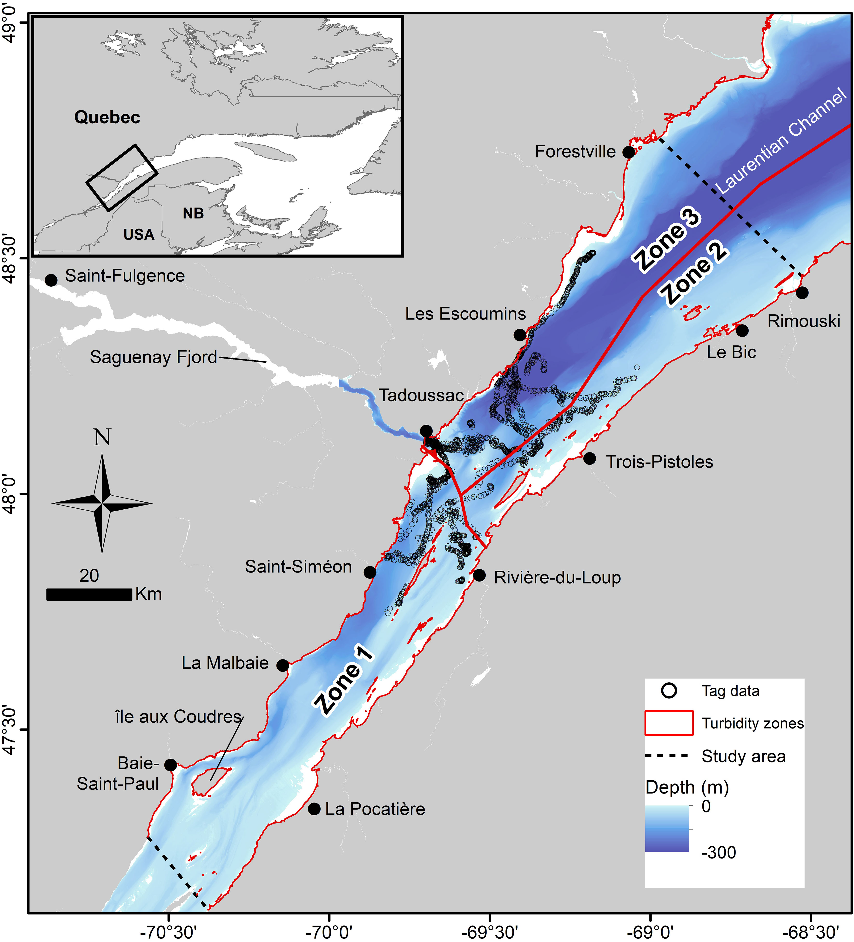
Figure 1 Movement patterns of the 27 St. Lawrence Estuary beluga equipped with archival tags (Tag data) that were retained for dive data analyses. Open circles represent sequential surface intervals for individual whales. Turbidity, estimated using a Secchi disk, increased from Zone 1 to Zone 3, with mid-range turbidity values of 2 m, 5 m, and 8 m, respectively (Kingsley and Gauthier, 2002). Dotted lines represent the limits of the population summer range (Michaud, 1993; Gosselin et al., 2017; St-Pierre et al., 2023).

Beluga habitat

The SLE beluga summer habitat is highly heterogeneous in bottom topography and turbidity. For example, the mouth of the Saguenay Fjord is a few tens of meters deep while 20 km to the north-east, the Laurentian Channel reaches more than 350 m (Figure 1). Turbidity also varies widely between sectors from 1.5 m to 11.6 m, with an average of 4 m during years with no excessive rainwater runoffs (Kingsley and Gauthier, 2002). This heterogeneity is likely to affect beluga availability to a camera or observer, and was accounted for in the current study by dividing the beluga summer habitat into three turbidity zones as per Gauthier (1999): Zone 1 has high turbidity (1.5–2.5 m) and is located in the upstream portion of the SLE (Upper Estuary); Zone 2 is of intermediate turbidity (3.5–6.5 m) and includes the southern half of the downstream portion of the SLE (Lower Estuary); Zone 3 has low turbidity (4.5–11.5 m) and encompasses the northern half of the Lower Estuary (Figure 1). On the assumption that white (adult) beluga can be detected at depths equivalent to Secchi-disk measurements (Kingsley and Gauthier, 2002), mid-range turbidity values were used as thresholds for beluga detection for the three zones (i.e., 2, 5 and 8 m, respectively). It is noteworthy that the relative use of these different zones of turbidity is not uniform among age and sex classes within the SLE beluga population (Michaud, 1993; Ouellet et al., 2021). In general, adult males are less often observed in the high turbidity zone than in the low turbidity one, whereas the opposite is true for adult females with calves and juveniles.

Areas of consistent summer aggregation within each of the three turbidity zones have been identified for SLE beluga using two long-term datasets and different statistical approaches, which yielded similar results (Lemieux Lefebvre et al., 2012; Mosnier et al., 2016). Areas of high density (AHD; 50% kernel density) identified by Mosnier et al. (2016) from aerial survey data were retained for this analysis as they offered a full coverage of the SLE beluga summer range; Lemieux-Lefebvre et al. (2012) identified high residency areas but covered only the core of their summer distribution. The specific functions associated with each of these AHD have not been identified. However, based on the reasonable assumption that foraging most often occurs in areas of AHD, with transit occurring more frequently outside these areas, availability to a passing aircraft should be less in AHD compared to transit areas (i.e., outside of AHDs), and even more so when beluga feed at depth and/or if they tend to remain closer to the surface when transiting. These assumptions are supported by the behaviors observed for SLE beluga inside and outside high residency areas (Lemieux Lefebvre et al., 2018). Availability may also decrease with increasing seafloor depth if beluga dive to the bottom, although the proportion of time an animal is available to a passing aircraft in this case would also depend on recovery time at the surface.

Estimating availability bias

For a given survey, event S represents the occurrence of a group of one or more beluga at or near the surface, and within field of view (McLaren, 1961). For visual surveys, availability a is represented as (S,x), the probability of such an occurrence at perpendicular distance x from the track-line (in m). Availability depends on beluga surface interval and dive durations (in s), and the amount of time a point at or near the water surface at distance x remains within observer view. Surface interval s and dive duration d are treated as a two-state continuous-time Markov process, and are estimated from individually-tracked beluga (Laake et al., 1997), such that:

$\begin{array}{ll}a(S,x)= \frac{s}{s+d}+\frac{d[1-e^{-w(x)/d}]}{s +d}& (1)\end{array}$

Equation 1 is the addition of two ratios or probabilities. The first ratio estimates the mean proportion of time during a dive cycle that an animal spends at the surface or the probability that an animal is at the surface when an aircraft arrives overhead. The second ratio estimates the probability of this animal appearing within an observer field-of-view during the aircraft passing, given the probability it was diving when the aircraft arrived. This second ratio is a function of w(x), the time any location at the surface at distance x remains in the observer view (in s), given the obstructed lateral view forward and backward (angle Ø₁ and Ø₂, respectively in radians), plane speed v (in m s^-1) and perpendicular distance x of the sighting (in m; Forcada et al., 2004; Gómez de Segura et al., 2006), where:

$\begin{array}{ll}w(x)= \frac{x}{v}[\cot ({\varnothing }_1)+\text{cot}({\varnothing }_2)]& (2)\end{array}$

For photographic surveys, only the probability that an animal is at or near the surface when the photo was taken is considered (i.e., first term in Equation 1), making availability necessarily lower for photographic than visual surveys. In this case, availability P is calculated as:

$\begin{array}{ll}P= \frac{s}{s+d}& (3)\end{array}$

Availability adjusted for photo overlap ($\overline{P}$), i.e., for the probability P_D of a beluga being imaged in at least one of two successive photographs, was calculated following Kingsley and Gauthier (2002). This probability P_D was estimated using tag data for the range of intervals between photos recorded during SLE beluga surveys (i.e., 3—19 s, for an achieved photo overlap of 0 to 39%; Lesage et al., 2023; St-Pierre et al., 2023).

Dive data collection

Availability bias for photographic and visual aerial surveys was estimated using high-resolution (0.25 m and 1 s) dive data from 27 beluga from the St. Lawrence Estuary (Mk8 recorders, Wildlife Computers, Redmond, WA). Tagging efforts spanned from June to September 2001—2005, and covered a variety of habitat used by all herd types and segments of the population (Figure 1*; Michaud, 1993; Mosnier et al., 2016; Ouellet et al., 2021). The suction cup attached archival tags were equipped with a 30 g radio transmitter (VHF, Telonics, Mesa, AZ), allowing remote tracking (400—600 m) with minimal effects on behavior (Blane and Jaakson, 1994). Tracking ceased either at dusk, when signal was lost, or when the tag came off. Tracked individuals were geolocated during each surface interval based on the animal’s relative distance (estimated by eye or range finder) and angle from the tracking vessel (using binoculars with compass), for which GPS position was logged every minute. Surface intervals with missing positions were interpolated from the preceding and following surface intervals when within 25 min from each other, i.e., SLE beluga maximum dive time based on tag data (Lemieux Lefebvre et al., 2018)¹.

Dive data analysis

Dive profiles and various statistics, including dive maximum depth and duration, and surface time (post-dive), were extracted using a custom-made program. Zero-offset correction was performed manually using Instrument Helper (Wildlife Computers Inc., Redmond, WA). The first and last dive cycles were removed as they were incomplete. Data was excluded when contact with the animal was lost for > 25 min, during periods outside survey hours (i.e., between dusk and dawn, which varied throughout the summer), or when individuals were in the Saguenay Fjord where counts are uncorrected for availability bias.

A dive was initially defined as any excursion below 0.5 m to capture series of short and shallow dives associated with surface intervals. Dive duration corresponded to the time elapsed between two successive surface intervals. A bout-ending criterion with the maximum likelihood estimation method (MLM) discriminated between dives and surface intervals (Langton et al., 1995; Luque and Guinet, 2007). An optimization algorithm (an extension of limited memory Broyden-Fletcher-Goldfarb-Shanno, or L-BFGS-B; Liu and Nocedal, 1989) was applied as part of the function to identify bouts. The upper and lower bound values were specified following Luque (2007).

Animals can be detected under water before they reach the surface, with detection depth varying with local turbidity. However, although beluga might dip momentarily (0.1—3.6 s on average) below the turbidity threshold during surface intervals and become invisible to a visual observer, these effects on availability are trivial even in the most turbid waters of the SLE, with time-in-view exceeding dip time at virtually all perpendicular distances (Lesage et al., 2023). Consequently, dip time was included as part of surface time for visual surveys, and as part of dive time for photographic surveys given that the latter are based on instantaneous detections.

Statistical analysis

The data set consisted of multiple geolocated dives (including dive and post-dive surface interval) from focally-tracked beluga with associated date, local time, and bathymetry (50 m horizontal resolution; Canadian Hydrographic Service), and location relative to turbidity zones (1, 2, or 3) and to areas of consistent aggregation (inside or outside AHD zones). Data were explored using standard procedures (Zuur et al., 2010) to ensure the absence of outliers in the data, and of collinearity, interaction or dependency (i.e. repeated measurements and spatial) among the observations of seafloor depth, behavior and Zone variables.

Dependency among successive dives when examining availability as a function of covariates was accounted for by including beluga focal ID as a random intercept in generalized additive mixed-effects models (GAMM). The validity of using a GAMM (and not a generalized linear mixed model) was assessed from the effective degree of freedom (edf) of the smooth term, where an edf > 1 indicates a non-linear relationship. A single response variable was considered for photographic surveys, i.e., the proportion of time a beluga was available during a dive cycle [i.e., P in Equation 3], whereas two response variables were considered for visual surveys [i.e., s and d were predicted using two separate GAMMs]. Resulting functions from the GAMMs incorporating each sighting’s location and associated characteristics were used to obtain sighting-specific s and d, then to estimate availability a(S,x) from Equation 1 (visual surveys), or were used to obtain sighting-specific P directly from Equation 3 (photographic surveys). Equation 1 also required information on perpendicular distance. When missing, sightings were georeferenced from the secondary observer data if available; otherwise, they were given a default value of 0 m (i.e., directly underneath the aircraft). Note that this was done only for estimating environmental and behavioral context of the sighting and not for estimating detection functions (details on how sightings with missing perpendicular distance were handled in abundance estimation are provided in St-Pierre et al., 2023). The relationship between residuals from the models using s or d as response variables was examined using scatterplots and Pearson correlation coefficients to ensure none existed and thus, that a multivariate model was not needed, and that incorporating functions for s and d into Equation 1 was appropriate.

Three covariates were considered in the GAMM models: Zone (1, 2, and 3) and location relative to AHD (inside or outside) were included as categorical covariates, whereas seafloor depth was included as a smooth term. Julian date and time-of-the-day were also considered for inclusion, but were ultimately excluded from the models; there were concerns that the uneven coverage of daytime hours due to short deployment times and span of tagging effort over several months would increase the likelihood of a few individuals biasing seasonal and diel effects. Initial models indicated that there were no spatial residual patterns, and we therefore refrained from using models with spatial dependency. Seven models were tested, representing all potential combinations of the three covariates; interactions were not included in the model (Supplementary 2 lists all the models tested). The highly restricted diving depth range used by several of the tagged individuals prevented testing a model with a random intercept and random smooths, i.e., with an overall and an animal-specific depth smoother.

Generalized additive mixed models were used to describe effects from environmental and behavioral features on P, s, and d in a three-step process (Figure 2). First, the potential heterogeneity in beluga surface s and dive times d as a result of the defined covariates was explored without consideration for turbidity, i.e., using 0.5 m as the threshold for defining a dive. These two response variables were continuous and positive; therefore, we used a Gamma GAMM with a log-link function. Thin plate regression splines were used for the smoothers and restricted maximum likelihood (REML) was used to estimate the smoothing parameters (Wood, 2018). The resulting models were defined as follows:

Figure 2

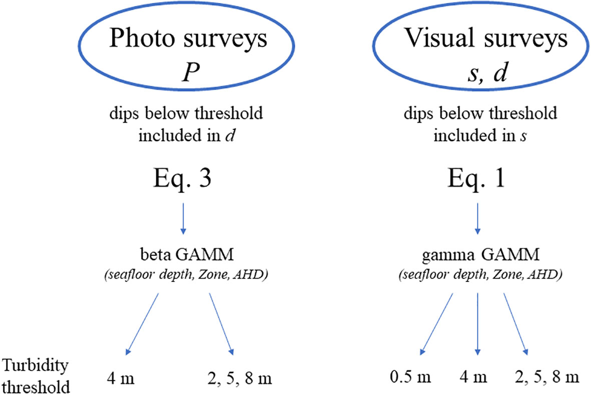
Figure 2 Analytical process for assessing effects from environmental and behavioral correlates on availability P during photographic surveys, and on surface time s and dive time d using generalized additive mixed effects models (GAMM). An example of all the models tested is available in Supplementary 2.

$$d_{ij}or{s}_{ij}\sim Gamma({\mu }_{ij},r)$$

$$E[d_{ij}]orE[s_{ij}]={\mu }_{ij}$$

$$\mathrm{var}[d_{ij}]orvar[s_{ij}]={\mu }_{ij}^2/r$$

$$u_{ij}=\exp (Intercept+Covariate{s}_{ij}+a_i)$$

$$a_i\sim N(0,{\sigma }^2)$$

where d_ij and s_ij are respectively, the estimated diving and surface interval durations for animal i and j^th dive, r is an unknown parameter controlling the variance, and a_i is a random intercept for animal i, which is assumed to be normally distributed with mean 0 and variance σ². This analysis was not conducted for photographic surveys given that time s, spent at the surface above 0.5 m, was generally ≤ 1 second for most dives, resulting in overly small P.

The added effect of turbidity on instantaneous availability P, and on s and d was then examined as a function of the same three covariates but this time, using 4 m as a threshold to define a dive, i.e., the average turbidity for the SLE beluga summer habitat (as in Kingsley and Gauthier, 2002). Given that P is a ratio ranging from 0 to 1, a beta GAMM with a logistic link function was used, such that:

$$P_{ij}\sim beta({\pi }_{ij},\theta )$$

$$E[P_{ij}]={\pi }_{ij}$$

$$\mathrm{var}[P_{ij}]={\pi }_{ij}\ast (1-{\pi }_{ij})/(1+\theta )$$

$$\mathrm{logit}({\pi }_{ij})=Intercept+Covariates+a_i$$

$$a_i\sim N(0,{\sigma }^2)$$

where P_ij is the proportion of time spent at the surface for animal i and jth dive, θ is an unknown parameter controlling the variance, and a_i is a random intercept for animal i, which is assumed to be normally distributed with mean 0 and variance σ².

In a third step, the added effect of location-specific turbidity was examined using a composite file consisting of the data reprocessed with a 2 m, 5 m and 8 m threshold to define a dive, and from which only sightings falling within the corresponding zone of turbidity (either Zone 1, 2 or 3, respectively) were extracted. Again, a beta GAMM was applied to P (photographic surveys), and a gamma GAMMs applied to s and d (visual surveys), to examine effects of the three covariates.

Models were fitted using the mgcv package (v1.8-40; Wood, 2011) in R software (v4.2.2, R Core Team, 2022). The main tool to find the optimal model was the Akaike information criterion (AIC); the simplest model was selected when difference in AIC was< 2. Model assumptions were verified by plotting Pearson residuals against fitted values, and against each covariate in the model and not in the model (Zuur et al., 2009). Spatial dependency of the residuals and the random effect was assessed using variograms (Schabenberger & Pierce, 2002).

Other factors affecting availability bias

The sensitivity of availability bias to survey design (photographic or visual), survey platform (with different field of view), distribution of sightings within the SLE beluga summer range, turbidity threshold, and each covariate was examined using the best model selected based on AIC and two datasets: 1) all photographic surveys conducted from 1990—2019 (n = 11), and 2) replicate visual surveys available from 2005 (n = 14), and 2019 (n = 4) (St-Pierre et al., 2023).

Because detection time varies with field-of-view and perpendicular distance from the aircraft, search patterns of an observer (i.e., limits on searching angles and distance from the aircraft) are expected to affect availability bias. To examine this question, we used the four surveys flown in 2019 with the Twin Otter, i.e., the platform offering the largest field-of-view, and estimated availability bias while varying the obstructed lateral view forward and backward (Ø₁ and Ø₂, respectively) for each sighting (Equation 2).

Estimating corrected group size and abundance

The estimated cluster size for a group seen in a specific location can then be corrected by producing for instance 5000 availability bias estimates (P or a(S, x)) for each sighting according to its specific seafloor depth, Zone, and AHD values by resampling model parameters (including random effects) using posterior simulation (Wood, 2018).

The 5000 P and a(S, x) obtained per sighting can then be used to generate 5000 corrected cluster size estimates $\overline{E}$ from observed group size E, as follows for photographic and visual surveys, respectively:

$\begin{array}{ll}\overline{E}=E·\frac{1}{\overline{P}}or\hspace{0.17em}\overline{E}=E·\frac{1}{a(S,x)}& (4)\end{array}$

These corrected cluster sizes then form the basis for estimating 5000 abundance estimates and associated variance, which can then be used as part of survey data analysis. An example of such an application can be found in St-Pierre et al. (accepted).

Accuracy and precision of abundance estimate and sample size

The sensitivity (i.e., relative precision and accuracy) of survey abundance estimates to the number of replicate surveys conducted was examined using a simulation-based power analysis. We based this analysis on replicate visual surveys conducted during three seasons: 14 surveys within a 29-day window in 2005, 6 surveys within a 16-day period in 2009, and 8 surveys conducted within a 22-day period in 2014 (total surveys = 28) (St-Pierre et al., 2023). Because each set of replicate surveys was conducted over a brief time window, we assumed that underlying “true abundance” remained constant within each year. We ensured that abundance estimates from sequential surveys each year were independent by testing for temporal autocorrelation using a Durbin-Watson test, the results of which were found to be non-significant (P = 0.9974, 0.6911, and 0.7364 for year 2005, 2009 and 2014 respectively). We next developed a simple Bayesian model to estimate the parameters for a process-based simulation model of replicate surveys to use as the basis for the power analysis. Using a process-based model to inform simulations provided several advantages: 1) it allowed us to generate large numbers of “new” survey data sets that would exhibit the same underlying variance structure as observed data sets; 2) we could more reliably extrapolate to smaller or larger numbers of survey replicates; and 3) we could assess the relationship between sample size and accuracy because simulated “true” values would be known (Zielinski and Stauffer, 1996; Arnold et al., 2011; Bellier et al., 2013). We structured the model to reflect two assumptions: 1) uncertainty in survey point estimates and their associated variance estimates are log-normally distributed (Fewster et al., 2009); and 2) variation across years in log abundance, and across surveys in log observer error, is normally distributed and thus appropriately modeled using a hierarchical design (Royle et al., 2007). Based on these assumptions, we define the following parameters: $\overline{\mu }$(the asymptotic median of log-transformed abundance estimates, averaged across years); σ_μ (which determines variation in log-transformed abundance estimates across years); μ_t (the asymptotic median log-transformed abundance estimate for year t); $\overline{\theta }$(the average value of θ_s,t, which is the log of parameter σ_s,t describing uncertainty in the abundance estimate for survey s); ψ (which determines variation in θ_s,t across surveys); β (the average effect of high-altitude surveys on log-transformed abundance estimates); and ϕ (a nuisance parameter allowing for differences between the computed estimation errors and the actual precision of replicate estimates). We assumed μ_t and θ_s,t were normally distributed hierarchical parameters:

$\begin{array}{ll}\begin{array}{l}{\mu }_t\sim normal(\overline{\mu },{\sigma }_{\mu })\\ {\theta }_{s,t}\sim normal(\overline{\theta },\psi )\end{array}& (5)\end{array}$

From the above-described base parameters we derived the estimate for asymptotic “true abundance” for year t using the standard equation for the mean of a log-normally distributed variable:

$\begin{array}{ll}E.tru{e}_t=\exp ({\mu }_t+\raisebox{1ex}{${\sigma }^2$}\!\left/ \!\raisebox{-1ex}{$2$}\right.),\sigma =\exp (\overline{\theta })& (6)\end{array}$

Additional derived parameters included the log uncertainty parameter for survey s in year t (σ_s,t = exp(θ_s,t)), which we converted to the expected estimator variance (V.est_s,t) using the standard equation for computing the variance of a log-normal variable:

$\begin{array}{ll}V.es{t}_{s,t}=[(\exp ({\sigma }_{s,t}^2)-1)·\exp (2·\log (E_{s,t})+{\sigma }_{s,t}^2)]·\varphi & (7)\end{array}$

In Equation 7, E_s,t represents the observed point estimate for survey s in year t, assumed to be drawn from a log-normal distribution:

$\begin{array}{ll}{E}_{s,t}\sim log\_normal({\mu }_t+\beta ·A_{s,t},{\sigma }_{s,t})& (8)\end{array}$

where A_s,t is a switch variable set to 0 for low altitude surveys (i.e., 305 m) and 1 for high altitude surveys (i.e., 457 m). The observed variance estimate for survey s in year t, V_s,t, was similarly assumed to be drawn from a log-normal distribution:

$\begin{array}{ll}{V}_{s,t}\sim log\_normal(\log (V.es{t}_{s,t}),{\sigma }_v)& (9)\end{array}$

where parameter σ_v described uncertainty in variance estimates.

We fit the above-described model to observed data variables E_s,t and V_s,t available from the 28 replicate surveys, using standard MCMC methods. We used R (R Core Team, 2022) and Stan software (Carpenter et al., 2017) to code and fit the model, saving 10,000 samples after a burn-in of 1000 samples. We set vague normal priors for $\overline{\mu },\overline{\theta }$, and β, a vague gamma prior (with mean of 1) for ϕ, and half-Cauchy priors for variance parameters σ_μ, σ_v and ψ (Gelman, 2006). These priors were selected to describe biological feasibility but provide minimal information relative to the observed data, and we ensured posteriors were distinct from priors by graphically comparing distributions. We evaluated model convergence by graphical examination of trace plots from five independent chains and by ensuring that the Gelman-Rubin convergence diagnostic (R-hat) was< 1.01 and the effective sample size (SS_eff) was > 500 for all fitted model parameters. We conducted graphical posterior predictive checking to evaluate model goodness of fit, ensuring that out-of-sample predictive distributions of abundance point estimates and variances were consistent with observed distributions. We also calculated Bayesian-P values (using the sum of Pearson residuals as the test statistic to be compared for observed vs. out-of-sample predicted data), with good model fit indicated by 0.1< Bayesian-P< 0.9. We used model results as the basis for a power analysis using iterated simulations of replicate surveys. Specifically, we drew parameter values from the joint posterior distribution of the fitted model and used these to generate simulated data sets of E_s and V_s by solving Equations 5–9. We created 1000 random data sets for sample sizes ranging from n = 1 to n = 20 replicate surveys. For each random data set, r, for sample size n, we calculated an abundance estimate ( ${\overline{E}}_{r,n}$) as the average of replicate survey point estimates (E_s), and we used the delta method to calculate the associated variance, ${\overline{V}}_{r,n}=(1/n^2)·(\Sigma V_S)$. We expressed the variance in terms of the coefficient of variance (CV), calculated as:

$\begin{array}{ll}C{V}_{r,n}=\raisebox{1ex}{$\sqrt{{\overline{V}}_{r,n}}$}\!\left/ \!\raisebox{-1ex}{${\overline{E}}_{r,n}$}\right.& (10)\end{array}$

We also computed a statistic describing relative accuracy, P.acc_n, which we calculated as the proportion of random point estimates (${\overline{E}}_{r,n}$) that differed by less than 15% from the “true abundance value” for the given simulation (calculated following Equation 6). We graphically examined the relationship between sample size and CV_r,n (reflecting the precision of abundance estimates) and P.acc_n (reflecting the accuracy of abundance point estimates).

Results

Twenty-seven of the 44 tags deployed could be used (one was lost, four recorded no data, three provided data solely in the Saguenay Fjord, and nine were deployed on beluga we lost sight of after tagging). Deployment duration among these 27 tags varied from 0.7 to 29.8 h. Once nighttime activity and other segments of unusable data were removed, there remained an average of 4.5 h of usable data per beluga (total: 134 h), with geolocations spread among the three zones (Figure 1).

Not all individuals visited the three zones, with 9, 8, and 21 out of 27 individuals visiting Zones 1, 2, and 3, respectively. Seafloor depth was unevenly distributed among these zones, being deeper on average in Zone 3 (Figure 1), and also deeper on average outside than inside AHD zones (95 m versus 37 m).

Correlations among variables

Data exploration revealed no specific problems with the data, other than interindividual variability in s and d and irregularity in spatial distribution, which were both expected. There was no relationship between s and d, with d [but not s] increasing with seafloor depth.

Using a 0.5 m threshold to define a dive, d and s were variable among the 27 tagged individuals, averaging 176.6 s (weighted SE = 12.6 s) and 51.6 s (weighted SE = 4.5 s), respectively. Beluga dove on average for similar durations in all three zones of their summer range; however, surface times were approximately 50% longer when in the deeper zone (Zone 3) than when in the other two zones (Supplementary Table 1A).

Overall, mean availability decreased with increasing turbidity. As expected, availability was higher for visual than photographic surveys due to dips below the turbidity threshold being logged as part of surface time for visual surveys, although values became almost identical between photographic and visual surveys at turbidity ≥ 4 m (Supplementary Table 1B).

Dive time

Environmental correlates of beluga dive times were the same regardless of whether effects of turbidity were considered (4-m average or zone-specific) or not (0.5 m) when estimating d. Specifically, variations in dive time were best explained by models including all three covariates, i.e., seafloor depth, Zone, and location relative to AHD (inside or outside) (Supplementary 2). Generally, d increased with seafloor depth down to about 50 m, with mild fluctuations at deeper depths (Figure 3), and was overall longer when belugas were inside AHDs or in Zone 1 (2 m turbidity threshold; the Upper Estuary). In all three models (0.5 m, 4 m, or zone-specific turbidity), a spatial dependency in Pearson residuals was noted up to approximately 400 m. The average net displacement speed for these tagged beluga (5.8 km h^-1; Lemieux Lefebvre et al., 2012) and mean dive durations (1.3—3.3 min depending on dive type; Lemieux Lefebvre et al., 2018) suggest that spatial dependency was greatly reduced beyond 2—3 consecutive dives or for dives performed > 4 min apart.

Figure 3

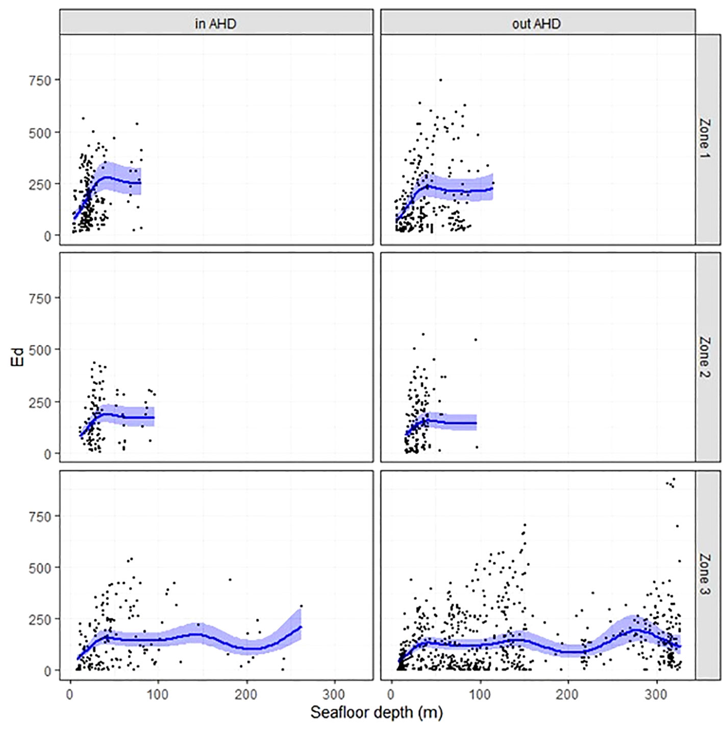
Figure 3 Mean dive time d (black curve) with 95% confidence interval (in blue) as a function of seafloor depth (m), Zone used, and whether animals were inside or outside AHD, and when considering zone-specific turbidity. Turbidity 2, 5 and 8 m correspond to Zones 1, 2 and 3, respectively. Black dots are raw data points.

Surface time

Variations observed in s were generally unrelated to covariates. Only when zone-specific turbidity was taken into account were Zone or seafloor depth slightly improving the fit to the data over the intercept-only model (Supplementary Table 3). However, the depth smoother was non-significant (P-value = 0.34), and the Zone effect arose mainly from a difference in s between the most and least turbid zones of the study area (Zones 1 and 3). Similar to d, there was a mild spatial dependency detected in Pearson residuals for s, also up to approximately 400 m, i.e., within the time frame for completing two consecutive dives.

Instantaneous availability (P)

When P was modulated according to local turbidity, influential covariates included seafloor depth, Zone, and whether animals were inside or outside AHD (Supplementary 4). Generally, instantaneous availability to a photographic survey decreased from Zone 3 to 1, decreased with seafloor depth, and was lower when animals were inside than outside AHDs (Figure 4).

Figure 4

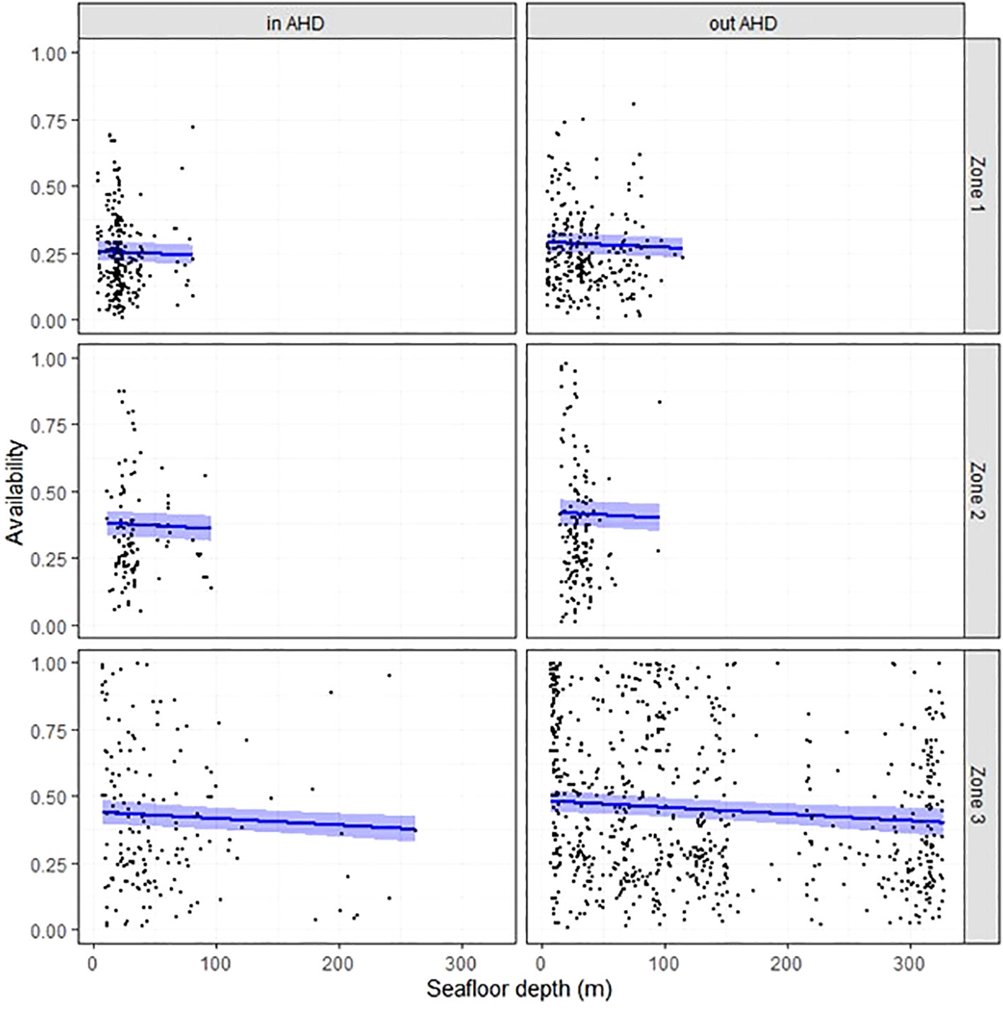
Figure 4 Instantaneous availability P (black curve) with 95% confidence interval (in blue) as a function of seafloor depth (m), Zone used, and whether animals were inside or outside AHD, and when considering zone-specific turbidity. Black dots are raw data points.

Model selection

The residuals from the optimal dive model d were unrelated (correlation ≤ 0.10) to the residuals of the optimal surface model s, confirming that a multivariate model for Equation 1 was unwarranted. Given pronounced differences in turbidity across the study area, models accounting for local turbidity (2, 5 and 8 m) were deemed more appropriate for our datasets than models assuming a uniform turbidity of 4 m. For photographic surveys, the selected model included seafloor depth, Zone and location relative to AHDs, with 26.4% of the deviance explained. For visual surveys, availability was estimated using the model without any covariates for s, and a model including all three covariates for d, which explained respectively 17.8% and 22.6% of the total deviance.

Sensitivity analysis

Beluga availability was on average higher during visual than photographic surveys (Figure 5). Estimates were also associated with a larger variance for visual than photographic surveys, likely as a result of variability in perpendicular distance among individual sightings and thus, variable time-in-view (see Equation 1). Survey platform for conducting visual surveys can also strongly affect availability through their specific angles of obstructed field-of-view: the Twin Otter with a 5°-5° forward-backward obstructed view resulted in a mean availability on average 54% higher (mean of 0.763, SE = 0.10 versus 0.496, SE = 0.007) than the Partenavia or Cessna 337 (mean 0.339, SE = 0.005), which had a 30°-20° forward-backward obstructed field-of-view (Figure 6). Using the 2019 Twin Otter visual survey data with various combinations of forward-backward obstructed field-of-view, our data indicates that the searching pattern of observers within the available field-of-view can have a substantial impact on estimated availability: a change from a 5°-5° to a 45°-45° or 0°-90° forward-backward obstructed field of view reduced mean availability by 43—46% (Figure 6). This analysis also highlights that applying an average availability from tag data a posteriori to mean abundance estimates instead of including this information in Equation 1 along with observed perpendicular distances and realistic field-of-view data, is likely to lead to an underestimation of availability and thus an overcorrection for this bias, especially for survey platforms with a wider field-of-view (Figure 6).

Figure 5

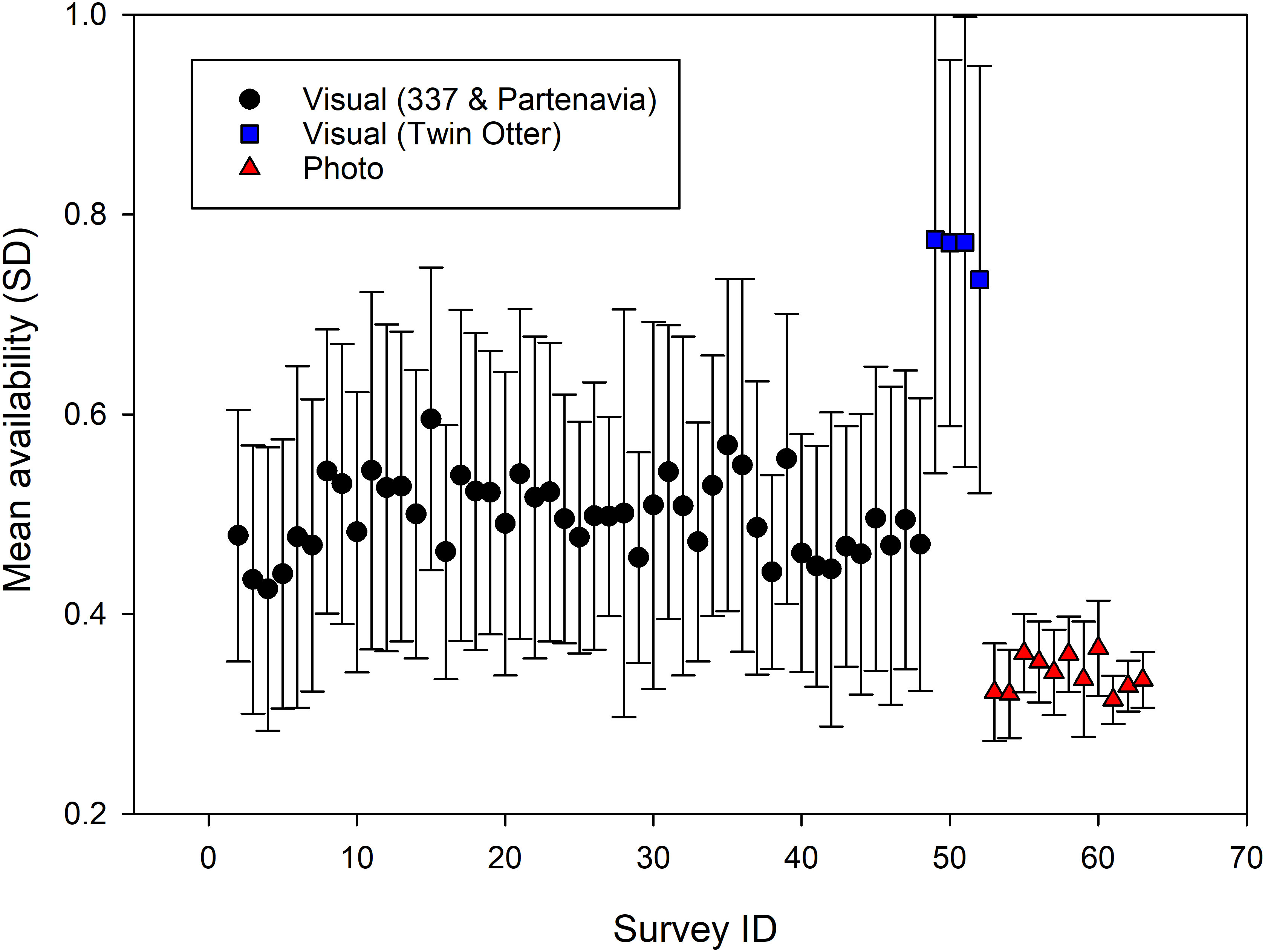
Figure 5 Mean availability for all visual (n = 52) and photographic (n = 11) surveys estimated using the best identified models (i.e., photographic surveys: a model accounting for location-specific turbidity, and including as covariates the seafloor depth, Zone, and location of sightings relative to areas of high densities (AHD); visual surveys: a model which takes into account the observer’s field of view, is estimated using a null model for surface time s, and one accounting for location-specific turbidity and incorporating the above three covariates for dive time d). Standard deviation (SD) is used here to highlight differences in the range of sighting-specific availability among surveys.

Figure 6

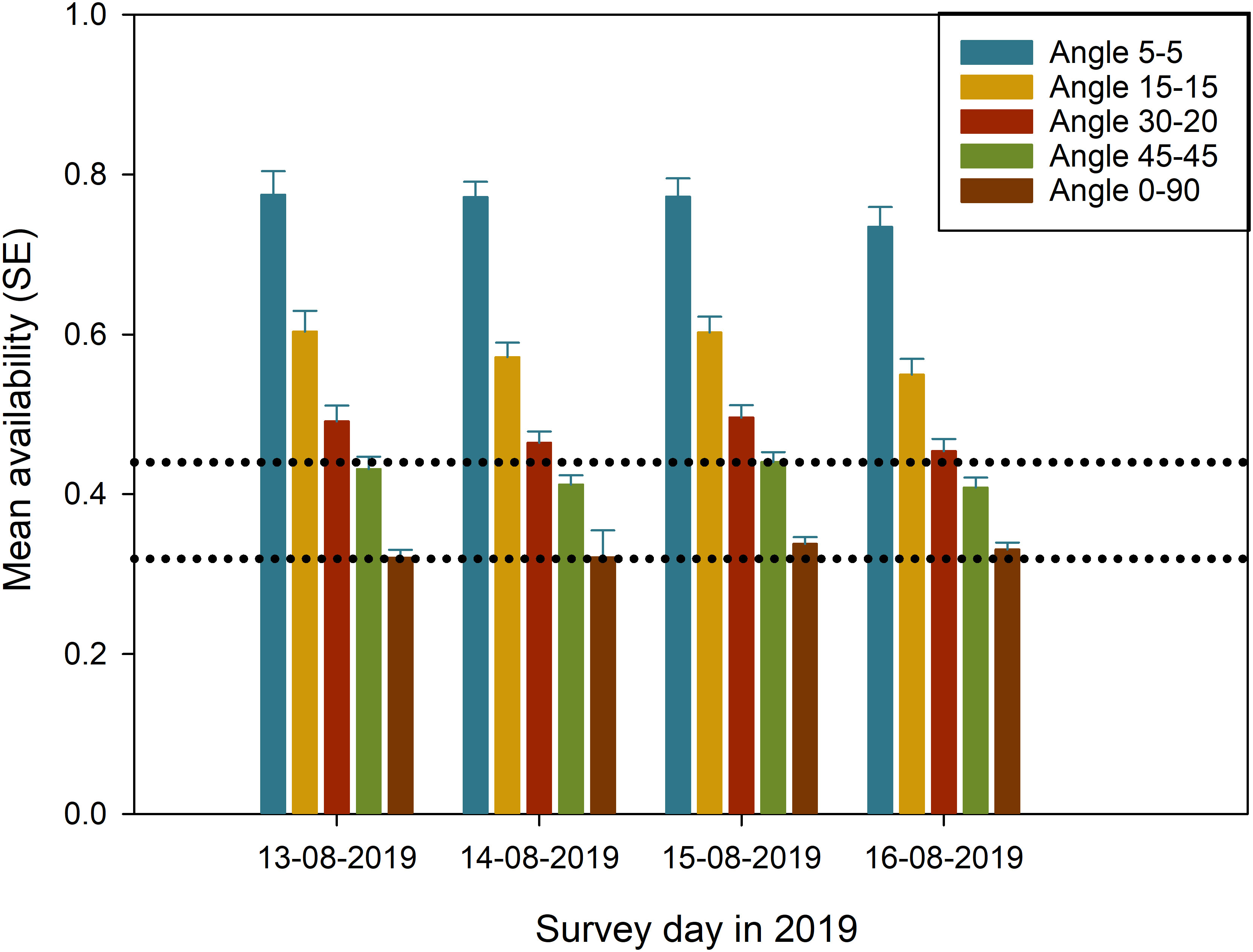
Figure 6 Effect of different combinations of forward-backward obstructed field-of-view on mean availability, illustrated using the best model for estimating availability and the four replicate visual surveys conducted using the Twin Otter in 2019 (St-Pierre et al., 2023). The horizontal dotted lines represent the range of mean availability obtained for the 51 visual surveys, estimated from the 27 tagged beluga while using turbidity thresholds varying from 2 m (lower line) to 8 m (upper line). Standard error (SE) is used here to highlight differences in mean availability among surveys.

Based on photographic survey data, the majority of beluga sightings in the SLE are made in the zone of highest turbidity during summer time: in all but three surveys (all in 2019), between 50 and 75% of the sightings were from Zone 1. This zone is also where mean availability was the lowest (i.e., 0.307 versus 0.363 and 0.399 for Zones 2 and 3, respectively); not accounting for zone effects for SLE would overestimate availability and thus, would lead to an underestimation of abundance.

Mean availability estimates were generally the lowest when all three covariates were included, i.e., the best model selected based on AIC. This was true for both photographic and visual surveys. Accounting for local turbidity (instead of using an average 4-m turbidity across the study area) increased availability by 2.6% and 1.6% on average for photographic and visual surveys, respectively. Adding one covariate at a time to these models revealed that the most influential covariate for both types of surveys was Zone; this variable which corresponds to the latent processes associated with using a specific zone, increased availability by 7.8% relative to turbidity-only (Null) models in the case of photographic surveys, and reduced availability by 3.8% relative to Null models in the case of visual surveys. Seafloor depth changed availability (either positively or negatively) by less than 2% in all but two [visual] surveys (mean: -0.1% and +2.0% relative to the Null models for photographic and visual surveys, respectively). In contrast, sighting’s location relative to AHDs had, to one exception, a consistently negative effect on availability (mean: -1.7 and -2.5% for photographic and visual surveys, respectively).

Overall, accounting for all covariates and local turbidity decreased availability by an average of 6.6% for photographic surveys, i.e., from a mean of 0.363 for the Null model with a 4-m average turbidity (range 0.335—0.381), to a mean of 0.339 for the model with all three covariates and location-specific turbidity (range 0.314—0.366) (Figure 7). Similarly, using the full model for the 14 visual surveys conducted in 2005 decreased availability by an average of 6.0% compared to the Null model using a 4-m average turbidity and no covariates (i.e., from a mean of 0.556 to 0.523). For a fictive population of 1000 individuals, using a 4-m Null model instead of the full model with location-specific turbidity would result on average in an under-estimation of the mean population size by approximately 190 and 115 individuals or 20% and 10%, for photographic and visual surveys, respectively.

Figure 7

Figure 7 Relative contribution of adjustments made to account for behavioral and environmental effects (red bars) on availability bias (blue bar), estimated from the 27 tagged beluga while accounting only for local turbidity and expressed as the correction (multiplier) applied to abundance estimate.

Precision and accuracy of abundance estimates

The Bayesian model examining the sensitivity of abundance estimates to the number of replicate surveys converged well and provided excellent fit to the data, with all R-hat values ≤ 1.01, a mean effective sample size of 2952 (minimum1433), and Bayesian-P values for posterior predictive checks of 0.403 for E_s,t and 0.503 for V_s,t. A summary of estimated model parameters is provided in Supplementary Table 5. Simulations based on this model indicated that the precision of abundance estimates (CV_r,n; Equation 10) decreased with sample size (number of survey reps), while estimation accuracy (P.acc_n) increased with sample size (Figures 8, 9). Because these functional relationships were non-linear, there was a large benefit of conducting more than 1 or 2 survey reps, but a declining benefit of conducting more than 5 to 10 survey reps. A sample size of 5 survey reps provided an estimated CV of 18% on average, while a sample size of 10 provided a CV of 13% (Figure 8). The probability that the resulting point estimate deviated by less than 15% from the true value for a sample size of 5 was 0.65, while the probability that the point estimate deviated by less than 15% from true value for a sample size of 10 was 0.76 (Figure 9).

Figure 8

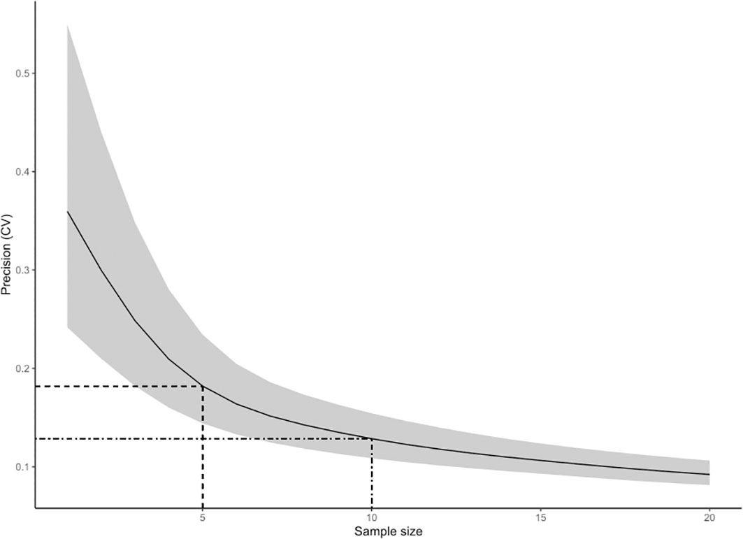
Figure 8 Plot of the precision of abundance estimates as a function of sample size (number of replicate surveys). The solid line indicates the mean expected coefficient of variation (CV) value associated with a given sample size, while the grey shaded band shows the 95% CI of the CV-sample size relationship. The dashed lines show the CV values associated with a sample size of 5 (CV = 18%) and a sample size of 10 (CV=13%).

Figure 9

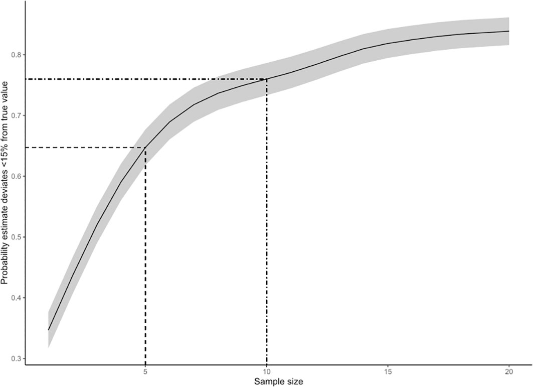
Figure 9 Estimation accuracy (defined as the proportion of simulations where the deviation between estimated abundance and “true abundance” was< 15% of true abundance) plotted as a function of sample size (number of replicate surveys). The solid line indicates the mean expected accuracy associated with a given sample size, while the grey shaded band shows the 95% CI of the accuracy-sample size relationship. The dashed lines show the proportional accuracy associated with a sample size of 5 replicate surveys (P.acc = 65%) and a sample size of 10 (P.acc = 76%).

Discussion

This study provided availability bias estimates for visual and photographic survey designs, and offered a comprehensive analysis of the relative influence of multiple methodological, environmental and behavioral factors on these estimates. Using an exceptional dataset, it also highlighted the large effect that a low number of survey replicates may have on accuracy and precision of abundance estimates.

Factors affecting availability bias

Although diving behavior is expected to vary as a function of habitat type, local depth, season, activity, group size, sex and age class (e.g., Würsig et al., 1984; Stockin et al., 2001; Southall et al., 2005; James et al., 2006; Pollock et al., 2006; Langtimm et al., 2011; Thomson et al., 2012), availability bias estimations are generally based on averages, without consideration for contextual variables (e.g., Barlow et al., 1988; Laake et al., 1997; Skaug et al., 2004; Doniol-Valcroze et al., 2020; Pike et al., 2020). Our results indicate that both dive time and instantaneous availability, but not surface time, were affected by local turbidity, seafloor depth, behavior (i.e., transit versus foraging), and latent processes that were habitat-specific. Our analysis confirmed that dives were longer when animals were inside compared to outside AHDs, consistent with the prediction that these areas are used for behaviors like foraging. However, the impact of adjusting availability bias to account for these effects was relatively minor compared to the influence exerted by survey design (photographic or visual), platform type, and observer search patterns (i.e., time-in-view).

The systematically higher availability bias observed for photographic compared to visual surveys underscores the importance of developing estimates that are specific to survey design (i.e., distinguishing instantaneous from non-instantaneous time-in-view). Using an instantaneous availability bias correction when detection process is non-instantaneous can positively bias abundance estimation (McLaren, 1961). For visual surveys, the strong dependency of availability bias on survey platform and obstructed field-of-view also raised questions about the influence of the search patterns of observers, and how availability and perception biases may counterbalance each other under different conditions. For instance, observers may be instructed to search the entire field-of-view available to them (e.g., St-Pierre et al., 2023) or instead, may be asked to restrict search area near the aircraft within a 0—90 degree forward angle (e.g., Hammond et al., 2013). More groups available at the surface may be missed in the first case, thus generating a higher perception bias. In counterpart, searching a wider field-of-view is likely to lead to a larger number of detections given the increase in detection time with distance from the aircraft. For instance, potential time-in-view within the typical observation distances for SLE beluga surveys (i.e., effective strip half width of ~ 600 m; e.g., Gosselin et al., 2017) can vary from ~ 0 s (on the trackline) to ~ 50 s for a Cessna 337 or Partenavia aircraft, and from 0 to ~ 270 s for a Twin Otter equipped with large bubble windows (Supplementary 2 in Lesage et al., 2023).

With distance sampling, a minimum of 60-80 observations are required to reliably estimate the detection function, and an even larger sample size is required when sampling species with a clumped distribution (Buckland et al., 2001). A basic assumption in distance sampling is that objects on the track line are detected with certainty, i.e., detection probability g(0) is 1.0 (Buckland et al., 2001). When the number of sightings is expected to be low, however, restricting search to an area near the aircraft or within a small angle may reduce the overall sample size, increase availability bias, and amplify the relative influence of individual sightings on the estimated detection function and abundance (Matthews et al., 2017). At high (or intermediate) density, searching efficiently close to the trackline is desirable despite higher availability bias correction, given that densities obtained from the reduced effective-strip-width can be expanded without bias to unsearched areas (Buckland et al., 2001). A potential caveat of such an approach, however, is related to cluster size estimation. At high density, observers continuing to monitor a large field-of-view may start rounding counts and thus be less accurate, or may not use the entirety of the field-of-view prescribed from limitation of the aircraft or specific guidance (Hobbs et al., 2000). Lumping multiple groups together at high density may inflate mean cluster size and associated variance (e.g., St-Pierre et al., 2023). However, this should theoretically be compensated by the encounter rate estimate and variance, and not result in any bias except if rounding or actual searching area is affected as mentioned above. This tendency may be exacerbated at short time-in-view, i.e., when searching within a small angular area near the aircraft. Overall, these findings indicate that decisions about the search area to cover during line-transect visual surveys can have notable impacts on abundance estimates and precision. They emphasize the importance of clearly defining field-of-view and search behavior to be adopted by observers at low and high densities for obtaining an unbiased estimate of availability bias (see Buckland et al., 2001 for strategies).

Availability bias corrections are often applied directly to total abundance as a proportion of time available to the survey platform, without consideration for the variability of time-in-view with perpendicular distance, i.e., not using Equation 1 (e.g., Hammond et al., 2013; Heide-Jørgensen et al., 2016; Marcoux et al., 2016; Pike et al., 2020). Our results further indicate that such an approach is likely to bias abundance estimates by an unknown and variable amount: a uniform but underestimated mean time-in-view would bias availability downward and abundance estimates upwards, whereas the reverse would lead to an underestimation of abundance. Not accounting for the variability in perpendicular distance among sightings when estimating availability will also likely lead to an underestimation of survey variance (McLaren, 1961; Laake et al., 1997).

Previous studies have highlighted the sensitivity of availability correction to turbidity for beluga surveys (e.g., Hobbs et al., 2000; Kingsley and Gauthier, 2002; Marcoux et al., 2016). A previous study of SLE beluga, observing the appearance and disappearance of groups of beluga of various sizes from a hovering helicopter, estimated instantaneous availability at 0.404 for areas with turbidity of 1 to 2 m, and at 0.543 for areas with turbidity > 4 m (Kingsley and Gauthier, 2002). In Cumberland Sound, availability based on daylight satellite telemetry data summarized by 6-h period (i.e., equivalent to instantaneous availability bias) varied from 0.224 to 0.485 for turbidity of 1 to 6 m, increasing abundance estimates by factors of 4.46—2.06 (e.g., Marcoux et al., 2016). Turbidity effects of a similar magnitude were noted in our study (Lesage et al., 2023, Supplementary 4B). However, the tendency of beluga in the SLE to occur in larger numbers in more turbid waters during surveys (Lesage et al., 2023) lowered their overall availability to survey platforms in our study.

Availability in our study was estimated from the behavior of individuals, and not groups as in Kingsley and Gauthier (2002), and was consistently lower (26—42%) than in the latter study. In both studies, data collection required use of an aircraft or vessel. While the helicopter altitude and vessel tracking distance were set to avoid behavioral reactions, a possible effect on beluga cannot be ruled out (Senigaglia et al., 2016). In the Kingsley and Gauthier (2002) study, an overestimation of availability could arise from selecting the first sighted beluga group if these individuals were engaged in more visible behaviors. Maximum group size was also set as the maximum number of beluga seen simultaneously; if not all beluga surfaced synchronously during surface intervals, then true group size was underestimated and visibility overestimated. Kingsley and Gauthier (2002) indicate that a recording session was initiated at the sight of a randomly chosen group, but provided no information as to when a session was terminated. If a session ended with the disappearance of a group and not with the initiation of a new post-dive surface interval, then surface time would be overrepresented relative to total observation time in each session, again biasing availability upwards. Tagging more than one individual in a group, although challenging logistically, or examining drone videos from multiple groups could have been instructive for understanding the synchrony of surface intervals within groups and the link between the probability of detecting a group during visual surveys versus individual behavior.

Availability bias in this study was obtained using 27 individually-tagged beluga. While this sample size is much larger than that of many studies having estimated availability of cetaceans from tag data (e.g., Heide-Jørgensen et al., 2012; Watt et al., 2015b; Matthews et al., 2017), a larger sample size, more evenly distributed sample among zones, and ideally included in a spatial model, would have been desirable. A sensitivity analysis using coastal dolphins suggests that availability is unlikely to have been biased by our sample size, but that an increase in sample size would have reduced variance further (Brown et al., 2023). While beluga tagging effort covered a large portion of the summer distribution of SLE beluga, it did not reach the two extremities of the SLE (Figure 1). There were also few individuals using Zone 3 that were sampled while over the Laurentian Channel where seafloor depth can reach more than 300 m; many whales were in the shallower waters at the head of the Channel. Beluga can reach depths of up to 1 000 m in other areas (Citta et al., 2013) and thus, are not limited by seafloor depth in the SLE. Beluga include benthic prey in their diet in the SLE (Vladykov, 1946; Lesage, 2021), and are expected to feed near the bottom at least in some of the AHD identified (Mosnier et al., 2016). In our study, dive duration increased with seafloor depth, although the effect of seafloor depth or of being in an AHD on availability appeared relatively weak. Given that 13—35% of the beluga may use the deep and clear waters of the Laurentian Channel at any one time (Michaud, 1993; see also Simard et al., 2023), increasing sample size for this region within zone 3 might enhance the relationship between availability and bottom depth and alter modelled estimates of availability. There is currently no information leading us to believe that beluga distribution or habitat use has changed substantially since the tagging study in the early 2000s. However, the extension of the tagging study to more recent years would confirm dive patterns and habitat use have remained consistent over time.

Another caveat of our study is related to not having sampled all age- and sex classes: females with newborn calves were required by research permit to be avoided. This segment of the population may be more available than others to survey platforms (by diving less often or to shallower depth), as suggested by diving records from beluga elsewhere (Heide-Jørgensen et al., 2001), and from other species such as coastal dolphins and North Atlantic right whales (Eubalaena glacialis) (Baumgartner and Mate, 2003; Brown et al., 2023). Not including females with calved in our sample may have biased availability downward.

An experiment in the SLE using grey and white beluga models has determined that white adults can be seen at Secchi-disk depth while grey juveniles can be seen on the film only at 50% or less of Secchi-disk depth (Kingsley and Gauthier, 2002). Similar results were obtained in the Arctic, where grey juveniles could only be seen at depths half that of adults, and dark-grey neonate models, not even at 20% of an adult depth (Richard et al., 1994). This means that grey juveniles might be under-represented on photographs by an unknown amount, leading to an underestimation of abundance. This bias might be less in Zone 3 where young and darker juveniles are less likely to be seen than in Zones 1 and 2 (Michaud, 1993; Ouellet et al., 2021). This aspect could be examined further by looking at differences in diving behavior of grey versus white individuals in the different zones, and by estimating the proportion of these classes in the population at the time surveys are conducted. High contrast imagery is often used during photographic surveys to increase detection of animals that are just below the water surface. For SLE beluga surveys, most animals appear white on such high contrast imagery, limiting its use to estimate the proportion of grey versus white animals in the population.

Precision and accuracy of abundance estimates

Ideally, abundance estimates should be derived from surveys targeting a single species to maximize data quality, and minimize uncertainty around estimates (Buckland et al., 2001), although surveying multiple species instead of focusing on a single species may or may not bias detection probability and abundance estimation depending on animal densities and degree of overlap (Lambert et al., 2019). It is also recommended for abundance estimates to have a precision (CV) of 0.3 or less if used for management advice (International Whaling Commission (IWC), 2003). Given the expectation of a decrease in the coefficient of variation (CV) with the increase in sample size (Kelley, 2007), repeated surveys may be necessary in some cases to increase precision of abundance estimates, and hence achieve greater power to detect an abundance trend (Gerrodette, 1987). However, surveys for marine mammals and cetaceans in particular, are logistically challenging and generally highly onerous. As a result, they are often multi-specific, with the number of replicate surveys being generally limited to one or two per year/season (e.g., Heide-Jørgensen et al., 2016; Doniol-Valcroze et al., 2020; Pike et al., 2020). Overall however, our analysis of an exceptional dataset of 8 to 14 replicate surveys per year conducted over a short period of time suggests that abundance estimates from single surveys, which is the rule for most cetacean surveys (e.g., Hammond et al., 2013; Taylor et al., 2017; Mannocci et al., 2018; Doniol-Valcroze et al., 2020; Pike et al., 2020), can be biased and imprecise. For social odontocetes such as SLE beluga, which occur at low densities with a highly clumped distribution, the results of single surveys may be too imprecise and unreliable as a basis for management advice (Nomani et al., 2012). These findings will be of particular relevance for species with similar distributions, including species of conservation concerns, i.e., that are at low abundance or harvested near maximum sustainable yield (e.g., Wade and DeMaster, 1999). It is also worth noting however, that there is a recognized need to improve the methodologies currently available for incorporating perception bias and sighting-specific availability bias and various other sources of uncertainty into the abundance estimation process. A more integrated approach to variance estimation may help reduce the number of surveys needed to achieve adequate precision and accuracy.

Conclusions

Accounting for behaviour and habitat-related effects on availability of marine mammals to survey platforms can improve accuracy of abundance estimates. Impacts of these factors are often minor relative to those exerted by survey design (photographic or visual), platform type, and observer search patterns (i.e., time-in-view), but may be more substantial when turbidity impairs animal detection during breathing sequences, or when strong behavioural or topographical variability is expected within the surveyed area. It is recommended that availability correction be applied to sightings while accounting for perpendicular distance (i.e., using Equation 1) and not just as a post hoc correction factor to surface abundance indices.

There are benefits and drawbacks to both visual and photographic surveys (reviewed in Hammond et al., 2021). Visual surveys are often associated with a smaller correction for availability than photographic surveys (unless search area is small), but require a much larger correction for perception bias than photographic surveys for which this bias may be negated by repeated photo readings. Photographic surveys are well adapted to census populations expected to be found at high densities; visual surveys may be more appropriate for populations occurring at low or more variable densities (Hammond et al., 2021). For visual surveys, the field-of-view should be adjusted to ensure high detection probability near the track line, even at high density, especially if surveys are not flown in a double-platform configuration to account for perception bias.

For some cetacean species, especially those with highly clumped distributions such as social odontocetes, a single survey may not achieve adequate precision and accuracy for abundance estimation. Replicate surveys can help improve estimation precision and accuracy in such cases: for SLE Beluga we found that 5 survey replicates were generally sufficient to meet management needs, although, this number might be less for other species or if a more integrated approach is adopted for variance estimation.

Data availability statement

The raw data supporting the conclusions of this article will be made available by the authors, without undue reservation.

Ethics statement

The animal study was approved by the Canadian Council on Animal Care/Maurice Lamontagne Institute Review Board. The study was conducted in accordance with the local legislation and institutional requirements.

Author contributions

VL: Conceptualization, Data curation, Formal analysis, Funding acquisition, Investigation, Methodology, Project administration, Supervision, Validation, Writing – original draft, Writing – review & editing. SW: Formal analysis, Funding acquisition, Investigation, Writing – review & editing. AZ: Formal analysis, Methodology, Writing – review & editing. J-FG: Conceptualization, Funding acquisition, Investigation, Methodology, Supervision, Writing – review & editing. MT: Formal analysis, Investigation, Methodology, Writing – review & editing. AM: Formal analysis, Methodology, Writing – review & editing. AS-P: Investigation, Methodology, Writing – review & editing. RM: Funding acquisition, Investigation, Writing – review & editing. DB: Investigation, Methodology, Supervision, Writing – review & editing.

Funding

The author(s) declare financial support was received for the research, authorship, and/or publication of this article. This project was funded by the Species at Risk and Whales Initiative program of Fisheries and Oceans Canada, and through scholarships to S.W. by the National Sciences and Engineering Reseach Council of Canada and the Fonds de recherche du Québec – Nature et technologie.

Acknowledgments

We would like to thank Thomas Doniol-Valcroze, Garry Stenson and Cortney Watt for their inputs on earlier data analysis. We also thank J-F. Ouellet for help with figures. This project was funded by the Species at Risk and Whales Initiative program of Fisheries and Oceans Canada, and through scholarships to SW by the National Sciences and Engineering Reseach Council of Canada and the Fonds de recherche du Québec – Nature et technologie.

Conflict of interest

Author AZ, from Highlands Statistics Ltd., was employed by Fisheries and Oceans Canada. Author MT was employed by the company Nhydra Ecological Consulting.

The remaining authors declare that the research was conducted in the absence of any commercial or financial relationships that could be construed as a potential conflict of interest.

Publisher’s note

All claims expressed in this article are solely those of the authors and do not necessarily represent those of their affiliated organizations, or those of the publisher, the editors and the reviewers. Any product that may be evaluated in this article, or claim that may be made by its manufacturer, is not guaranteed or endorsed by the publisher.

Supplementary material

The Supplementary Material for this article can be found online at: https://www.frontiersin.org/articles/10.3389/fmars.2024.1289220/full#supplementary-material

Footnotes

1. ^ V. Lesage, Fisheries and Oceans Canada, Mont-Joli, QC.

References

Arnold B. F., Hogan D. R., Colford J. M., Hubbard A. E. (2011). Simulation methods to estimate design power: an overview for applied research. BMC Med. Res. Methodol. 11, 94. doi: 10.1186/1471-2288-11-94

PubMed Abstract | CrossRef Full Text | Google Scholar

Barlow J., Oliver C. W., Jackson T. D., Taylor B. L. (1988). Harbor porpoise abundance estimation for California and Washington II. Aerial surveys. Fish. Bull. 86, 433–444.

Google Scholar

Baumgartner M. F., Mate B. R. (2003). Summertime foraging ecology of North Atlantic right whales. Mar. Ecol. Prog. Ser. 264, 123–135. doi: 10.3354/meps264123

CrossRef Full Text | Google Scholar

Bellier E., Monestiez P., Certain G., Chadœuf J., Bretagnolle V. (2013). Reducing the uncertainty of wildlife population abundance: model-based versus design-based estimates. Environmetrics 24, 476–488. doi: 10.1002/env.2240

CrossRef Full Text | Google Scholar

Blane J. M., Jaakson R. (1994). The impact of ecotourism boats on the St Lawrence beluga whales. Environ. Conserv. 21, 267–269. doi: 10.1017/S0376892900033282

CrossRef Full Text | Google Scholar

Brack I. V., Kindel A., Oliviera L. F. B. (2019). Detection errors in wildlife abundance estimates from Unmanned Aerial Systems (UAS) surveys: Synthesis, solutions, and challenges. Methods Ecol. Evol. 9, 1864–1873. doi: 10.1111/2041-210X.13026

CrossRef Full Text | Google Scholar

Bröker K. C. A., Hansen R. G., Leonard K. E., Koski W. R., Heide-Jorgensen M.-P. (2019). A comparison of image and observer based aerial surveys of narwhal. Mar. Mamm. Sci. 35, 1253–1279. doi: 10.1111/mms.12586

CrossRef Full Text | Google Scholar

Brown A. M., Allen S. J., Kelly N., Hodgson A. J. (2023). Using unoccupied aerial vehicles to estimate availability and group size error for aerial surveys of coastal dolphins. Remote Sens. Ecol. Conserv. 9, 340–353. doi: 10.1002/rse2.313

CrossRef Full Text | Google Scholar

Buckland S. T., Anderson D. R., Burnham K. P., Laake J. L., Borchers D. L., Thomas L. (2001). Introduction to Distance Sampling: Estimating Abundance of Biological Populations (Oxford: Oxford University Press).

Google Scholar

Buckland S. T., Anderson D. R., Burnham K. P., Laake J. L., Borchers D. L., Thomas L. (2004). Advanced distance sampling: Estimating abundance of biological populations (Oxford, UK: Oxford University Press).

Google Scholar

Burt M. L., Borchers D. L., Jenkins K. J., Marques T. A. (2014). Using mark recapture distance sampling methods on line transect surveys. Methods Ecol. Evol. 5, 1180–1191. doi: 10.1111/j.1365-2664.2012.02150.x

CrossRef Full Text | Google Scholar

Cardinale B., Primack R., Murdoch J. (2019). Conservation Biology (Oxford: Oxford University Press), 584.

Google Scholar

Carpenter B., Gelman A., Hoffman M. D., Lee D., Goodrich B., Betancourt M., et al. (2017). Stan: A probabilistic programming language. J. Stat. Software 76 (1), 1–32. doi: 10.18637/jss.v076.i01

CrossRef Full Text | Google Scholar

Caughley G. (1974). Bias in aerial survey. J. Wildlife. Manage. 38, 921–933. doi: 10.2307/3800067

CrossRef Full Text | Google Scholar

Citta J. J., Suydam R. S., Quakenbush L. T., Frost K. J., O’Corry-Crowe G. M. (2013). Dive behaviour of Eastern Chukchi beluga whales (Delphinapterus leucas), 1998-2008. Arctic 66, 389–406. doi: 10.14430/arctic4326

CrossRef Full Text | Google Scholar

Dombroski J. R. G., Parks S. E., Nowacek D. P. (2021). Dive behavior of North Atlantic right whales on the calving ground in the Southeast USA. Endang. Species. Res. 46, 35–48. doi: 10.3354/esr01141

CrossRef Full Text | Google Scholar

Doniol-Valcroze T., Gosselin J.-F., Pike D. G., Lawson J. W., Asselin N. C., Hedges K., et al. (2020). Distribution and abundance of the Eastern Canada – West Greenland bowhead whale population based on the 2013 High Arctic Cetacean Survey. NAMMCO. Sci. Publications., 11. doi: 10.7557/3.5315

CrossRef Full Text | Google Scholar

Doniol-Valcroze T., Lesage V., Giard J., Michaud R. (2011). Optimal foraging theory predicts diving and feeding strategies of the largest marine predator. Behav. Ecol. 22, 880–888. doi: 10.1093/beheco/arr038

CrossRef Full Text | Google Scholar

Edwards H. H., Pollock K. H., Ackerman B. B., Reyholds J. E. III, Powell J. A. (2007). Estimation of detection probability in manatee aerial survey at a winter aggregation site. J. Wildlife. Manage. 71, 2052–2060. doi: 10.2193/2005-645

CrossRef Full Text | Google Scholar

Elphick C. S. (2008). How you count counts: The importance of methods research in applied ecology. J. Appl. Ecol. 45, 1313–1320. doi: 10.1111/j.1365-2664.2008.01545.x

CrossRef Full Text | Google Scholar

Fewster R. M., Buckland S. T., Burnham K. P., Borchers D. L., Jupp P. E., Laake J. L., et al. (2009). Estimating the encounter rate variance in Distance Sampling. Biometrics 65, 225–236. doi: 10.1111/j.1541-0420.2008.01018.x

PubMed Abstract | CrossRef Full Text | Google Scholar

Forcada J., Gazo M., Aguilar A., Gonzalvo J., Fernández-Contreras M. (2004). Bottlenose dolphin abundance in the NW Mediterranean: Addressing heterogeneity in distribution. Mar. Ecol. Prog. Ser. 275, 275–287. doi: 10.3354/meps275275

CrossRef Full Text | Google Scholar

Foster M. S. (2012). “Standard techniques for inventory and monitoring,” in Reptile biodiversity: standard methods for inventory and monitoring. Eds. McDiar-mid R. W., Foster M. S., Guyer C., Gibbons J. W., Chernoff N. (Berkeley, California, USA: University of California Press), 205–271.

Google Scholar

Fuentes M. M. P. B., Bell I., Hagihara R., Hamann M., Hazel J., Huth A., et al. (2015). Improving in-water estimates of marine turtle abundance by adjusting aerial survey counts for perception and availability biases. J. Exp. Mar. Biol. Ecol. 471, 77–83. doi: 10.1016/j.jembe.2015.05.003

CrossRef Full Text | Google Scholar

Gauthier I. (1999). Estimation de la visibilité aérienne des bélugas du Saint-Laurent et les conséquences pour l’évaluation des effectifs. MSc thesis. Université du Québec à Rimouski, 104.

Google Scholar

Gelman A. (2006). Prior distributions for variance parameters in hierarchical models. Bayesian Anal. 1 (3), 515–533.

Google Scholar

Gerrodette T. (1987). A power analysis for detecting trends. Ecology 68, 1364–1372. doi: 10.2307/1939220

CrossRef Full Text | Google Scholar

Gómez de Segura A., Tómas J., Pedraza S. N., Crespo E. A., Raga J. A. (2006). Abundance and distribution of the endangered loggerhead turtle in Spanish Mediterranean waters and the conservation implications. Anim. Conserv. 9, 199–206. doi: 10.1111/j.1469-1795.2005.00014.x

CrossRef Full Text | Google Scholar

Gosselin J.-F., Hammill M. O., Lesage V. (2007). Comparison of photographic and visual abundance indices of belugas in the St. Lawrence Estuary in 2003 and 2005. DFO. Can. Sci. Advis. Sec. Res. Doc. 2007/025.

Google Scholar

Gosselin J.-F., Hammill M. O., Mosnier A. (2014). Summer abundance indices of St. Lawrence Estuary beluga (Delphinapterus leucas) from a photographic survey in 2009 and 28 line transect surveys from 2001 to 2009. DFO. Can. Sci. Advis. Sec. Res. Doc. 2014/021.

Google Scholar

Gosselin J.-F., Hammill M. O., Mosnier A., Lesage V. (2017). Abundance index of St. Lawrence Estuary beluga, Delphinapterus leucas, from aerial visual surveys flown in August 2014 and an update on reported deaths. DFO. Can. Sci. Advis. Sec. Res. Doc. 2017/019.

Google Scholar

Gosselin J.-F., Lesage V., Robillard A. (2001). Population index estimate for the beluga of the St Lawrence River Estuary in 2000. DFO. Can. Sci. Advis. Sec. Sci. Advis. Rep. 2001/049.

Google Scholar

Hammond P. S., Francis T. B., Heinemann D., Long K. J., Moore J. E., Punt A. E., et al. (2021). Estimating the abundance of marine mammal populations. Front. Mar. Sci. 8. doi: 10.3389/fmars.2021.735770

CrossRef Full Text | Google Scholar

Hammond P. S., Macleod K., Berggren P., Borchers D. L., Burt M. L., Cañadas A., et al. (2013). Cetacean abundance and distribution in European Atlantic shelf waters to inform conservation and management. Biol. Conserv. 164, 107–122. doi: 10.1016/j.biocon.2013.04.010

CrossRef Full Text | Google Scholar

Heide-Jørgensen M.-P., Hammeken N., Dietz R., Orr J., Richard P. R. (2001). Surfacing times and dive rates for narwhals (Monodon monoceros) and belugas (Delphinapterus leucas). Arctic 54, 284–298. doi: 10.14430/arctic788

CrossRef Full Text | Google Scholar

Heide-Jørgensen M.-P., Hansen R. G., Fossette S., Nielsen N. H., Borchers D. L., Stern H., et al. (2016). Rebuilding beluga stocks in West Greenland. Anim. Conserv. 20, 282–293. doi: 10.1111/acv.12315

CrossRef Full Text | Google Scholar

Heide-Jørgensen M.-P., Laidre K. L., Hansen R. G., Burt M. L., Simon M., Borchers D. L., et al. (2012). Rate of increase and current abundance of humpback whales in West Greenland. J. Cetacean. Res. Manage. 12, 1–14. doi: 10.47536/jcrm.v12i1.586

CrossRef Full Text | Google Scholar

Hiby L. (1999). “The objective identification of duplicate sightings in aerial survey for porpoise,” in Marine Mammal Survey and Assessment Methods. Eds. Garner G. W., Armstrup S. C., Laake J. L., Manly B. F. J., McDonald L. L., Robertson D. G. (Balkema, Rotterdam), 179–189.

Google Scholar

Higdon J. W., Ferguson S. H. (2017). Database of aerial surveys and abundance estimates for beluga and narwhals in the Canadian Arctic. Can. Tech. Rep. Fish. Aquat. Sci. 3211, v + 48.

Google Scholar

Hobbs R. C., Waite J. M., Rugh D. J. (2000). Beluga, Delphinapterus leucas, group sizes in Cook Inlet, Alaska, based on observer counts and aerial video. Mar. Fish. Rev. 62, 46–59.

Google Scholar

Holt R. S., Gerrodette T., Cologne J. B. (1987). Research vessel survey design for monitoring dolphin abundance in the eastern tropical Pacific. Fish. Bull. 85, 435–446.

Google Scholar

Hornby C. A., Hoover C., Iacozza J., Barber D. G., Loseto L. L. (2016). Spring conditions and habitat use of beluga whales Delphinapterus leucas during arrival to the Mackenzie River. Polar. Biol. 39, 2319–2334. doi: 10.1007/s00300-016-1899-9

CrossRef Full Text | Google Scholar

International Whaling Commission (IWC) (2003). International whaling commission. 2003b. Report of the scientific committee. J. Cetacean. Res. Manage. Suppl.) 5, 1–92.

Google Scholar

James M. C., Ottensmeyer C. A., Eckert S. A., Myers R. A. (2006). Changes in diel diving patterns accompany shifts between northern foraging and southward migration in leatherback turtles. Can. J. Zool. 84, 754–765. doi: 10.1139/z06-046

CrossRef Full Text | Google Scholar

Kelley K. (2007). Sample size planning for the coefficient of variation from the accuracy in parameter estimation approach. Behav. Res. Meth 39, 755–766.

Google Scholar

Kingsley M. C. S. (1993). Census, trend and status of the St Lawrence beluga population in 1992. Can. Tech. Rep. Fish. Aquat. Sci. 1938, vi + 17.

Google Scholar

Kingsley M. C. S. (1996). Estimation d’un indice d’abondance de la population de bélugas du Saint-Laurent en 1995. Can. Tech. Rep. Fish. Aquat. Sci. 2117, 42.

Google Scholar

Kingsley M. C. S. (1999). Population indices and estimates for the belugas of the St. Lawrence Estuary. Can. Tech. Rep. Fish. Aquat. Sci. 2266, 27.

Google Scholar

Kingsley M. C. S., Gauthier I. (2002). Visibility of St. Lawrence belugas to aerial photography, estimated by direct observation. NAMMCO. Sci. Publ. 4, 259–270. doi: 10.7557/3.2848

CrossRef Full Text | Google Scholar

Kingsley M. C. S., Hammill M. O. (1991). Photographic census surveys of the St. Lawrence beluga population 1988 and 1990. Can. Tech. Rep. Fish. Aquat. Sci. 1776, 19.

Google Scholar

Laake J. L., Calambokidis J., Osmek S. D., Rugh D. J. (1997). Probability of detecting harbor porpoise from aerial surveys: Estimating g(0). J. Wildlife. Manage. 61, 63–75. doi: 10.2307/3802415

CrossRef Full Text | Google Scholar

Lambert C., Authier M., Dorémus G., Gilles A., Hammond P., Laran S., et al. (2019). The effect of a multi-target protocol on cetacean detection and abundance estimation in aerial surveys. R. Soc. Open Sci. 6, 190296. doi: 10.1098/rsos.190296

PubMed Abstract | CrossRef Full Text | Google Scholar

Langtimm C. A., Dorazio R. M., Stith B. M., Doyle T. J. (2011). New aerial survey and hierarchical model to estimate manatee abundance. J. Wildlife. Manage. 75, 399–412. doi: 10.1002/jwmg.41

CrossRef Full Text | Google Scholar

Langton S. D., Collett D., Sibly R. M. (1995). Splitting behaviour into bouts: A maximum likelihood approach. Behaviour 132, 781–799. doi: 10.1163/156853995X00144

CrossRef Full Text | Google Scholar

Lemieux Lefebvre S., Lesage V., Michaud R., Humphries M. M. (2018). Classifying and combining herd surface activities and individual dive profiles to identify summer behaviours of beluga (Delphinapterus leucas) from the St. Lawrence Estuary, Canada. Can. J. Zool. 96, 393–410. doi: 10.1139/cjz-2017-0015

CrossRef Full Text | Google Scholar

Lemieux Lefebvre S., Michaud R., Lesage V., Berteaux D. (2012). Identifying high residency areas of the threatened St. Lawrence beluga whale from fine-scale movements of individuals and coarse-scale movements of herds. Mar. Ecol. Prog. Ser. 450, 243–257. doi: 10.3354/meps09570

CrossRef Full Text | Google Scholar

Lesage V. (2021). The challenges of a small population exposed to multiple anthropogenic stressors and a changing climate: the St. Lawrence Estuary beluga. Polar. Res. 40, 5523. doi: 10.33265/polar.v40.5523

CrossRef Full Text | Google Scholar

Lesage V., Wing S., Zuur A. F., Gosselin J.-F., Mosnier A., St-Pierre A. P., et al. (2023). Environmental factors and behaviour of St. Lawrence Estuary beluga generate heterogeneity in availability bias for photographic and visual aerial surveys. DFO. Can. Sci. Advis. Sec. Res. Doc. 2023/046.

Google Scholar

Liu D. C., Nocedal J. (1989). On the limited memory method for large scale optimization. Math. Program B. 45, 503–528. doi: 10.1007/BF01589116

CrossRef Full Text | Google Scholar

Loseto L. L., Richard P., Stern G. A., Orr J., Ferguson S. H. (2006). Segregation of Beaufort Sea beluga whales during summer. Can. J. Zool. 84, 1743–1751. doi: 10.1139/z06-160

CrossRef Full Text | Google Scholar

Lowry L. F., Citta J. J., O’Corry-Crowe G., Quakenbush L. T., Frost K. J., Suydam R., et al. (2019). Distribution, abundance, harvest and status of western Alaska beluga whale, Delphinapterus leucas, stock. Mar. Fish. Rev. 81, 54–71. doi: 10.7755/MFR.81.3–4.2

CrossRef Full Text | Google Scholar

Luque S. P. (2007). Diving behaviour analysis in R. R. News 7, 8–14.

Google Scholar

Luque S. P., Guinet C. (2007). A maximum likelihood approach for identifying dive bouts improves accuracy, precision, and objectivity. Behaviour 144, 1315–1332. doi: 10.1163/156853907782418213

CrossRef Full Text | Google Scholar

Mannocci L., Robert J. J., Halpin P., Authier M., Boisseau O., Bradai M. N., et al. (2018). Assessing cetacean surveys through the Mediterranean Sea: a gap analysis in environmental space. Scient. Rep. 8, 3126. doi: 10.1038/s41598-018-19842-9

CrossRef Full Text | Google Scholar

Marcoux M., Young B. G., Asselin N. C., Watt C. A., Dunn J. B., Ferguson S. H. (2016). Estimate of Cumberland Sound beluga (Delphinapterus leucas) population size from the 2014 visual and photographic aerial survey. DFO. Can. Sci. Advis. Sec. Res. Doc. 2016/037.

Google Scholar

Marsh H., Sinclair D. F. (1989). Correcting for visibility bias in strip transect aerial surveys of aquatic fauna. J. Wildlife. Manage. 53, 1017–1024. doi: 10.2307/3809604

CrossRef Full Text | Google Scholar

Martin A. R., Smith T. G. (1999). Strategy and capability of wild belugas, Delphinapterus leucas, during deep, benthic diving. Can. J. Zool. 77, 350–360. doi: 10.1139/z99-129

CrossRef Full Text | Google Scholar

Matthews C. J. D., Watt C. A., Asselin N. C., Dunn J. B., Young B. G., Montsion L. M., et al. (2017). Estimated abundance of the Western Hudson Bay beluga stock from the 2015 visual and photographic aerial survey. DFO. Can. Sci. Advis. Sec. Res. Doc. 2017/061.

Google Scholar

McLaren I. A. (1961). Methods of determining the numbers and availability of ringed seals in the eastern Canadian Arctic. Arctic 14, 162–175. doi: 10.14430/arctic3671

CrossRef Full Text | Google Scholar

Michaud R. (1993). Distribution estivale du béluga du Saint-Laurent; synthèse 1986 à 1992. Rapp. Tech. Can. Sci. Halieut. Aquat. 1906.

Google Scholar

Michaud R. (2005). “Sociality and ecology of the odontocetes,” in Sexual segregation in vertebrates: Ecology of the two sexes. Eds. Ruckstuhl K. E., Neuhaus P. (Cambridge, UK: Cambridge University Press), 303–326.

Google Scholar

Mosnier A. R., Larocque R., Lebeuf M., Gosselin J.-F., Dubé S., Lapointe V., et al. (2016). Définition et caractérisation de l’habitat du béluga (Delphinapterus leucas) de l’estuaire du Saint-Laurent selon une approche écosystémique. Secr. Can. Consult Sci. du. MPO. Doc. rech. 2016/052.

Google Scholar

Mosnier A., Lesage V., Gosselin J.-F., Lemieux Lefebvre S., Hammill M. O., Doniol-Valcroze T. (2010). Information relevant to the documentation of habitat use by St. Lawrence beluga (Delphinapterus leucas), and quantification of habitat quality. DFO. Can. Sci. Advis. Sec. Res. Doc. 2009/098.

Google Scholar

Nomani S. Z., Oli M. K., Carthy R. R. (2012). Line transects by design: The influence of study design spatial, distribution and density of objects on estimates of abundance. Open Ecol. J. 5, 25–44. doi: 10.2174/1874213001205010025

CrossRef Full Text | Google Scholar

Nykänen M., Jessopp M., Doyle T. K., Harman L. A., Cañadas A., Breen P., et al. (2018). Using tagging data and aerial surveys to incorporate availability bias in the abundance estimation of blue sharks (Prionace glauca). PloS One 13, e0203122. doi: 10.1371/journal.pone.0203122

PubMed Abstract | CrossRef Full Text | Google Scholar

Orgeret F., Cox S. L., Weimerskirch H., Guinet C. (2019). Body condition influences ontogeny of foraging behavior in juvenile southern elephant seals. Ecol. Evol. 9, 223–236. doi: 10.1002/ece3.4717

PubMed Abstract | CrossRef Full Text | Google Scholar

Ouellet J.-F., Michaud R., Moisan M., Lesage V. (2021). Estimating the proportion of a beluga population using specific areas from connectivity patterns and abundance indices. Ecosphere 12, e03560. doi: 10.1002/ecs2.3560

CrossRef Full Text | Google Scholar

Pike D. G., Gunnlaugsson T., Mikkelsen B., Halldórsson S. D., Víkingsson G. A., Acquarone M., et al. (2020). Estimates of the abundance of cetaceans in the central North Atlantic from the T-NASS Icelandic and Faroese ship surveys conducted in 2007. NAMMCO. Sci. Publ. 11. doi: 10.7557/3.5269

CrossRef Full Text | Google Scholar

Pirotta E., New L., Marcoux M. (2018). Modelling beluga habitat use and baseline exposure to shipping traffic to design effective protection against prospective industrialization in the Canadian Arctic. Aquat. Conserv.: Mar. Freshw. Ecosyst. 28, 713–722. doi: 10.1002/aqc.2892

CrossRef Full Text | Google Scholar

Pollock K., Marsh H., Lawler I. R., Aldredge M. W. (2006). Estimating animal abundance in heterogeneous environments: An application to aerial surveys for dugongs. J. Wildlife. Manage. 70, 255–262. doi: 10.2193/0022-541X(2006)70[255:EAAIHE]2.0.CO;2

CrossRef Full Text | Google Scholar

R Core Team (2022). R: A language and environment for statistical computing (Vienna, Austria: R Foundation for Statistical Computing). Available at: https://www.R-project.org/.

Google Scholar

Richard P. R., Weaver P. A., Dueck L., Barber D. A. (1994). Distribution and relative abundance of Canadian high Arctic narwhals (Monodon monoceros) in August 1984. Meddr. Gr¢nland. Biosci. 39, 41–50. doi: 10.7146/mogbiosci.v39.142533

CrossRef Full Text | Google Scholar

Royle J. A., Kéry M., Gautier R., Schmid H. (2007). Hierarchical spatial models of abundance and occurrence from imperfect survey data. Ecol. Monogr. 77, 465–481. doi: 10.1890/06-0912.1

CrossRef Full Text | Google Scholar

Schabenberger O., Pierce F. (2002). Contemporary statistical models for the plant and soil sciences (Boca Raton: CRC Press), 760.

Google Scholar

Schreer J. F., Kovacs K. M. (1997). Allometry of diving in air-breathing vertebrates. Can. J. Zool. 75, 339–358. doi: 10.1139/z97-044

CrossRef Full Text | Google Scholar

Schweder T., Øien N., Høst G. (1991). Estimates of the detection probability for shipboard surveys of northeastern Atlantic minke whales, based on a parallel ship experiment. Rep. Int. Whal. Comm. 41, 417–432.

Google Scholar

Seber G. A. F. (1982). The estimation of animal abundance and related parameters (London: Charles Griffin).

Google Scholar

Senigaglia V., Christiansen F., Bejder L., Gendron D., Lundquist D., Noren D. P., et al. (2016). Meta-analyses of whale-watching impact studies: comparisons of cetacean responses to disturbance. Mar. Ecol. Prog. Ser. 542, 251–263. doi: 10.3354/meps11497

CrossRef Full Text | Google Scholar

Simard Y., Giard S., Roy N., Aulanier F., Lesage V. (2023). Mesoscale habitat use by St. Lawrence Estuary beluga over the annual cycle from an acoustic recording network. J. Acoust. Soc. Am. 154, 635–649. doi: 10.1121/10.0020534

PubMed Abstract | CrossRef Full Text | Google Scholar

Skaug H. J., Øien N., Schweder T., Bøthun G. (2004). Abundance of minke whales (Balaenoptera acutorostrata) in the Northeast Atlantic: Variability in time and space. Can. J. Fish. Aquat. Sci. 61, 870–886. doi: 10.1139/f04-020

CrossRef Full Text | Google Scholar

Slooten E., Dawson S. M., Rayment W. J. (2004). Aerial surveys for coastal dolphins: abundance of Hector’s dolphins off the South Island west coast, New Zealand. Mar. Mamm. Sci. 20, 477–490. doi: 10.1111/j.1748-7692.2004.tb01173.x

CrossRef Full Text | Google Scholar

Smith A. J., Higdon J. W., Richard P., Orr J., Bernhardt W., Ferguson S. H. (2017). Beluga whale summer habitat associations in the Nelson River estuary, western Hudson Bay, Canada. PloS One 12, e0181045. doi: 10.1371/journalpone.0181045

PubMed Abstract | CrossRef Full Text | Google Scholar

Southall E. J., Sims D. W., Metcalfe J. D., Doyle J. I., Fanshawe S., Lacey C., et al. (2005). Spatial distribution patterns of basking sharks on the European shelf: preliminary comparison of satellite-tag geolocation, survey and public sightings data. J. Mar. Biol. Assoc. UK. 85, 1083–1088. doi: 10.1017/S0025315405012129

CrossRef Full Text | Google Scholar

Stenson G. B., Hammill M. O., Lawson J. W., Gosselin J.-F. (2014). Estimating pup production of Northwest Atlantic harp seals, Pagophilus groenlandicus, in 2012. DFO. Can. Sci. Advis. Sec. Res. Doc. 2014/057.

Google Scholar

Stockin K. A., Fairbairns R. S., Parsons E. C. M., Sims D. W. (2001). Effects of diel and seasonal cycles on the dive duration of the minke whale (Balaenoptera acutorostrata). J. Mar. Biol. Assoc. UK. 81, 189–190. doi: 10.1017/S0025315401003630

CrossRef Full Text | Google Scholar

St-Pierre A. P., Lesage V., Mosnier A., Tinker M. T., Gosselin J.-F. (2023). Summer abundance estimates for St. Lawrence Estuary beluga (Delphinapterus leucas) from 52 visual line transect surveys and 11 photographic surveys conducted from 1990 to 2022. DFO. Can. Sci. Advis. Sec. Res. Doc. 2023/048.

Google Scholar

Sucunza F., Danilewicz D., Cremer M., Andriolo A., Zerbini A. N. (2018). Refining estimates of availability bias to improve assessments of the conservation status of an endangered dolphin. PloS One 13 (3), e0194213. doi: 10.1371/journal.pone.0194213

PubMed Abstract | CrossRef Full Text | Google Scholar

Taylor B. L., Martinez M., Gerrodette T., Barlow J. (2007). Lessons from monitoring trends in abundance of marine mammals. Mar. Mamm. Sci. 23, 157–175. doi: 10.1111/j.1748-7692.2006.00092.x

CrossRef Full Text | Google Scholar

Taylor B. L., Rojas-Bracho L., Moore J., Jaramillo-Legorreta A., Ver Hoef J. M., Cardenas-Hinojosa G., et al. (2017). Extinction is imminent for Mexico’s endemic porpoise unless fishery bycatch is eliminated. Conserv. Lett. 10, 588–595. doi: 10.1111/conl.12331

CrossRef Full Text | Google Scholar

Thomson J. A., Cooper A. B., Burkholder D. A., Heithaus M. R., Dill L. M. (2012). Heterogeneous patterns of availability for detection during visual surveys: Spatiotemporal variation in sea turtle dive-surfacing behaviour on a feeding ground. Methods Ecol. Evol. 3, 378–387. doi: 10.1111/j.2041-210X.2011.00163.x

CrossRef Full Text | Google Scholar

Vladykov V. D. (1946). “Études sur les mammifères aquatiques,” in IV. Nourriture du marsouin blanc (Delphinapterus leucas) du fleuve et du golfe Saint-Laurent (Department of Fisheries, Province of Quebec), 129.

Google Scholar

Wade P. R., DeMaster D. P. (1999). “Determining the optimum interval for abundance surveys,” in Marine mammal survey and assessment methods. Eds. Garner G. W., Amstrup S. C., Laake J. L., Manly B. J. F., McDonald L. L., Robertson D. G. (the Netherlands: Balkema, Rotterdam), 53–66.

Google Scholar

Watt C. A., Marcoux M., Asselin N. C., Orr J. R., Ferguson S. H. (2015b). Instantaneous availability bias correction for calculating aerial survey abundance estimates for narwhal (Monodon monoceros) in the Canadian High Arctic. DFO. Can. Sci. Advis. Sec. Res. Doc. 2015/044.

Google Scholar

Watt C. A., Marcoux M., Leblanc B., Ferguson S. H. (2015a). Instantaneous availability bias correction for calculating aerial survey abundance estimates for bowhead whales (Balaena mysticetus) in the Canadian High Arctic. DFO. Can. Sci. Advis. Sec. Res. Doc. 2015/046.

Google Scholar

Whitehead H., Weilgart L. (1991). Patterns of visually observable behaviour and vocalizations in groups of female sperm whales. Behaviour 118, 275–296. doi: 10.1163/156853991X00328

CrossRef Full Text | Google Scholar

Williams B. K., Nichols J. D., Conroy M. J. (2002). “Analysis and management of Animal Populations,” in Modeling, Estimation, and Decision Making (San Diego: Academic Press).

Google Scholar

Wood S. N. (2011). Fast stable restricted maximum likelihood and marginal likelihood estimation of semiparametric generalized linear models. J. R. Stat. Soc. B. 73, 3–36. doi: 10.1111/j.1467-9868.2010.00749.x

CrossRef Full Text | Google Scholar

Wood S. N. (2018). Generalized Additive Models: An Introduction with R. 2nd Edition (Boca Raton: Chapman & Hall/CRC).

Google Scholar

Würsig B., Dorsey E. M., Fraker M. A., Payne R. S., Richardson W. J., Wells R. S. (1984). Behavior of bowhead whales, Balaena mysticetus, summering in the Beaufort Sea: surfacing, respiration, and dive characteristics. Can. J. Zool. 62, 1910–1921. doi: 10.1139/z84-281

CrossRef Full Text | Google Scholar

Zielinski W. J., Stauffer H. B. (1996). Monitoring martes populations in California: survey design and power analysis. Ecol. Appl. 6, 1254–1267. doi: 10.2307/2269605

CrossRef Full Text | Google Scholar

Zuur A. F., Ieno E. N., Elphick C. S. (2010). A protocol for data exploration to avoid common statistical problems. Methods Ecol. Evol. 1, 3–14. doi: 10.1111/j.2041-210X.2009.00001.x

CrossRef Full Text | Google Scholar

Zuur A. F., Ieno E. N., Walker N., Saveliev A. A., Smith G. M. (2009). Mixed effects models and extensions in ecology (New York: Springer).

Google Scholar