Estimating three-dimensional current fields in the Yeosu Bay using coastal acoustic tomography system

1 Introduction

1.1 Background

Coastal acoustic tomography (CAT) is an emerging technology designed to monitor coastal environments. This technology evolved from ocean acoustic tomography, which was originally developed by Munk and Wunsch (1979), and has been adapted for coastal applications. Unlike traditional in-situ current measurement methods such as stationary or intermittent sectional observations, CAT can estimate time-varying temperature and current fields using reciprocally transmitted acoustic signals between CAT stations. This approach is cost-effective and provides valuable observational results for many coastal regions (Kaneko et al., 2020).

Research estimating the current field using CAT has primarily focused on calculating the depth-averaged horizontal two-dimensional current field. Park and Kaneko (2001) presented an inverse method for estimating the current field by applying the L-curve method to CAT data. Subsequently, current field measurements were conducted by applying this inverse method to CAT observations among multiple stations (e.g., Yamoaka et al., 2002; Zhu et al., 2012; Zhang et al., 2017). Additionally, research has been conducted to estimate horizontal current fields considering coastal effects using coast-fitting tomographic inversion in semi-enclosed seas (Chen et al., 2020), as well as assimilating CAT observation data into numerical models to reproduce current fields (Park and Kaneko, 2000; Zhu et al., 2021). As the need for three-dimensional (3-D) current field observations in coastal areas has increased, 3-D current fields have been derived by assimilating CAT observation data into a numerical model with unstructured triangular grids (Zhu et al., 2017). However, 3-D current field estimation from inverse analysis rather than from the data assimilation method using a numerical ocean model with a large number of calculations and a complex calculation procedure has not been reported so far. Kaneko et al. (2020) proposed a method for 3-D mapping of the current field from the sound speed deviation data of CAT through a two-step inversion procedure from vertical to horizontal slices. This method is feasible when multi-ray identification of 2^nd or 3^rd rays which pass through multiple layers along the sound transmission path is possible. However, because this is almost impossible in coastal areas, where the distances between stations are short and the water depth is shallow, this method cannot be applied to CAT data.

In this study, we combine an artificial intelligence (AI) model and an empirical orthogonal function (EOF) with an existing inverse method to develop a new 3-D current field estimation method. This method has the advantage of fully reflecting the current pattern of the study area by applying EOF and simultaneously reducing the number of unknowns during inverse analysis, thereby enabling the effective estimation of currents in underdetermined systems with a minimal number of observations. Moreover, by employing a pre-trained AI model, this method allows the rapid estimation of the 2-D current field along the section between two CAT stations using single-ray acoustic observations of CAT. The newly developed method was applied to in-situ CAT data to demonstrate its applicability for continuous current field monitoring using the CAT system in coastal seas.

1.2 Study area

The study area was Yeosu Bay, located in the southern part of the Republic of Korea, as shown in Figure 1. Because Yeosu Bay is characterized by shallow depth, complex coastline, and active ship traffic, there has been a growing need for real-time monitoring of current fields in this region. This region is dominated by tidal currents and shows a typical two-layer structure with opposing flows; the upper-layer currents from the estuarine area flow southward, whereas the lower-layer currents flow northward (Pritchard, 1952; Lee and Kim, 2007).

Figure 1

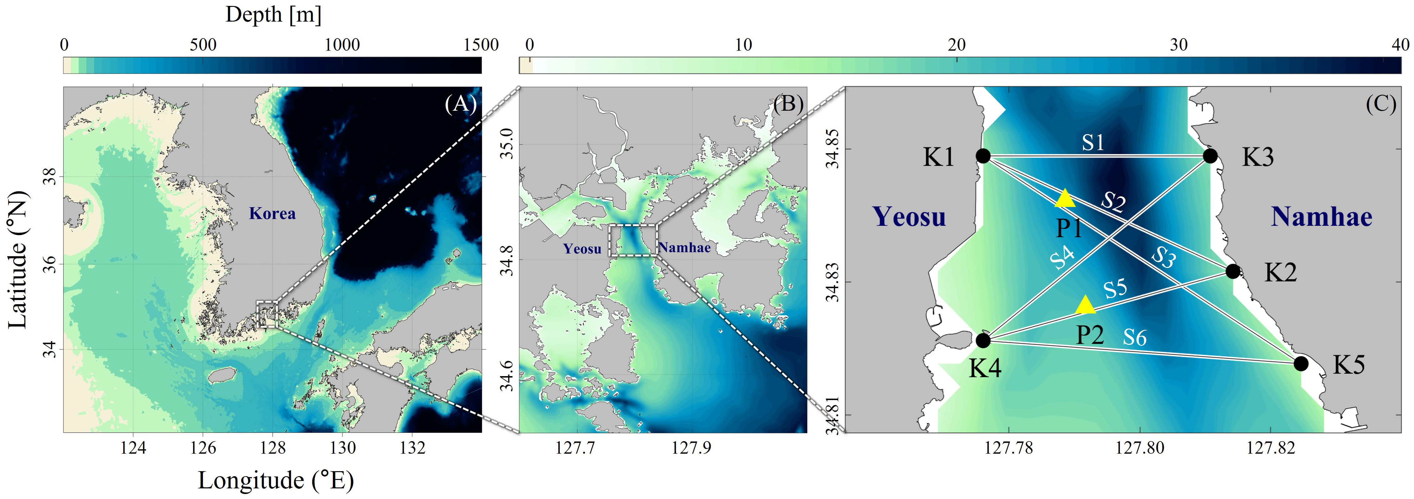
Figure 1 Study area in the Yeosu Bay, Korea. (A) Map of the Korean Peninsula. (B) Map of Yeosu and Namhae located in the South Sea of Korea, including the (C) Yeosu Bay. Black dots in (C) indicate the CAT stations and the lines connected between the CAT stations are paths for acoustic transmission simulation. Yellow triangles in (C) indicate ADCP mooring sites (P1, P2).

In this study, the target area for current field estimation was selected as a channel with a high current velocity in Yeosu Bay (Figure 1C). Six transmission paths were established by designating two stations on the west (Yeosu side) and three stations on the east (Namhae side) and connecting the stations to the west and east, as presented in Figure 1C. The ‘Transmission Path’ S1 is between stations K1 and K3, S2 is between K1 and K2, S3 is between K1 and K5, S4 is between K4 and K3, S5 is between K4 and K2, and S6 is between K4 and K5. Hereinafter, the term ‘path’ follows the definition of ‘Transmission Path.’ The CAT stations obtained through the high-resolution ocean numerical model results coincide with the actual locations where in-situ CAT observations are being conducted. The in-situ observation stations are the land station, except K4 which is located on the barge. This study utilized a numerical ray tracing model to validate the newly developed 3-D current field estimation method. The newly developed method was applied to in-situ CAT data. The locations of the five CAT stations and the two Acoustic Doppler Current Profiler (ADCP) mooring sites are listed in Table 1.

Table 1

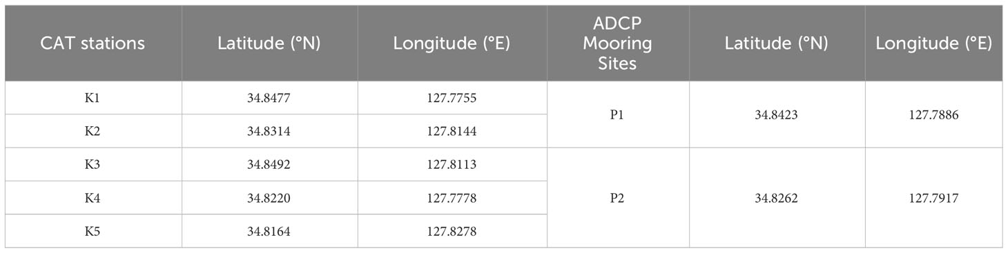
Table 1 Locations of CAT stations and ADCP mooring sites.

2 Data and methods

2.1 Data

The data utilized in this study were data assimilated real-time ocean prediction modeling results from the Korea Operational Oceanography System (KOOS), which was developed by the Korea Institute of Ocean Science and Technology (KIOST). The temporal and spatial resolutions of the data and their durations are summarized in Table 2. The depth, current, sea level, temperature, and salinity results from the KOOS model were used as input data for the Bellhop ray tracing model (Porter, 2011). The current data from the KOOS model were used for the EOF analysis, and the eigenvectors derived from the EOF analysis were used for inverse estimation. Additional information regarding the input data used to train the AI model is presented in Supplementary Figures 1, 2.

Table 2

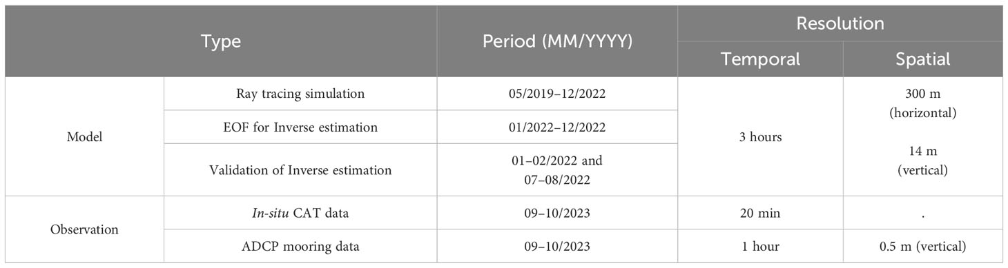
Table 2 Summary of the data used in this study.

The in-situ application of the method was performed from September to October 2023 and validated against the ADCP mooring data at P1 and P2 (Figure 1C). The observation periods are presented in Table 2. The temporal resolutions were 20 min and 1 h, respectively, which are finer than that of the KOOS model; however, because the inverse method was built using the KOOS model, the in-situ application was also performed at 3-hour intervals.

2.2 Methods

In this study, the 3-D current field was estimated using the following three procedures. First, the reciprocal travel time difference (Δt) of each transmission path is computed through the ray tracing simulation. Second, Δt^′ for each layer and path are computed using the AI model, which is trained with Δt. Finally, inverse analysis was applied to each layer, resulting in a 3-D current field consisting of five layers.

2.2.1 Ray tracing simulation

The first step, the ray tracing simulation, uses a numerical ray tracing model ‘Bellhop’ to calculate the reciprocal travel time difference (Δt). The Bellhop model requires the following files as inputs: ‘.bty’, ‘.ati’, ‘.env’, and ‘.ssp’. The ‘.bty’ and ‘.ati’ files contain information on the topography and water level of the simulation path. The ‘.ssp’ file contains the sound speed and current along the transmission path. The sound speed used here was calculated using temperature and salinity using the equation from Del Grosso (1974). The ‘.env’ file contains parameters such as the depth of the source and receiver, number of beams, and launching degree. The Bellhop model uses these input data to output the travel time (t_i) between two stations from the current [u(x,y,z,t)] and sound speed [C(x,y,z,t)].

$${\mathit{\text{t}}}_{\mathit{\text{i}}}={\oint }_{{\mathit{\text{L}}}_{\mathit{\text{i}}}}^{ }\frac{\mathit{\text{ds}}}{\mathit{\text{C}}(\mathit{\text{x}},\mathit{\text{y}},\mathit{\text{z}},\mathit{\text{t}})+\mathit{\text{u}}(\mathit{\text{x}},\mathit{\text{y}},\mathit{\text{z}},\mathit{\text{t}})·\mathit{\text{n}}}$$

If the Bellhop model is performed for both directions, we get the reciprocal travel time (t⁺, t^–) from ‘. ray’ file. The final output of the ray tracing simulation is reciprocal travel time difference (Δt = t⁺– t^–). The ray tracing simulation is performed for each of the six transmission paths to obtain a time series of six reciprocal travel time differences (Δt₁ –Δt₆). Supplementary Figure 1 shows a detailed flowchart including the input and output data of the Bellhop model and the final output. Supplementary Figure 3 shows time series of ray tracing. ‘Calculated v’ is the current made from the ray tracing results, and ‘model v’ is the KOOS model current data. They show similar trends of mean velocity, implying that Δt is mainly affected by velocity along the path.

2.2.2 AI model

In the second process, the range-averaged currents in the five layers in the vertical section of the six transmission paths were obtained using the AI model. The input data for the AI model are presented in Supplementary Table 1, and the data locations are provided in Supplementary Figure 2. The data duration was approximately four years (May 2019 to April 2023), including the period used for training the AI model. The collected data were preprocessed to normalize and enhance their learning ability. The other designs used for training the AI model are presented in Supplementary Table 2. The design of the “training process” is as follows. The “test set” consisted of January–February and July–August 2022, the periods covered by the inverse analysis. During this period, no learning took place, and only real simulations were conducted. For all periods except the “test set,” about 2/3 of the data is “training set,” and the remaining 1/3 is “validation set.” Independent training is conducted for each of the three non-overlapping “validation sets.” The initial values of these models were randomized, and training was performed three times for each model, resulting in nine ensemble model sets. The final model results were obtained by averaging nine ensemble models. This ensemble process provided robust model results. Although the direction-based loss function typically uses the mean squared error (MSE), the model used in this study focuses on learning the upper modes by utilizing the EOF results as learning weights, resulting in the establishment of an optimized direction-based loss function.

The AI model was designed to estimate the principal component (PC) time series of EOF using appropriate AI model layers for input data with different structures and dimensions (see Supplementary Figure 4). To simulate the current caused by the difference in sea level between the southern and northern parts of Yeosu Bay, sea level data were only extracted at the southern and northern boundaries of the domain. Because the two boundaries have different lengths of data (11 and 8 nodes, respectively), a dense layer was utilized to have the same length of nodes, and then applied to a 1-D convolutional long short-term memory (ConvLSTM1D) filter to handle the spatial dimension. The calculation of the sea level difference was not entirely dependent on the neural network, and a subtraction layer was added to directly calculate the difference between the two lines. The dimension of sea level data passed through ConvLSTM1D is compressed from [time, space, feature] to [time, feature]. Ocean data, atmospheric data, and Bellhop model output data have dimensions of [time, feature], resulting in merging with compressed sea level data. The merged data pass through a dense layer and a hyperbolic tangent (nonlinear activation function), and then pass through an LSTM layer that handles the time series. In this procedure, the time dimension was removed, leaving the [feature] dimension. The tidal-current input field consisting of [latitude, longitude, depth, (U, V)] dimensions were passed through the 3-D convolutional layer and compressed into [feature] dimensions. Finally, the layer is merged with the layer that passes through the LSTM and is compressed into three dense layers to obtain the length of the PC time series (1^st–10^th modes) of the EOF. The PC time series estimated using this process was then dot-produced using the eigenvectors obtained from the EOF analysis to obtain the current fields along the six vertical sections.

The validation results are presented in Supplementary Table 3 and Supplementary Figures 5, 6. Supplementary Table 3 shows the average root-mean-squared error (RMSE) of the along-path velocity for the six vertical sections compared with the true value, and Supplementary Figure 5 shows the RMSE fields of the six vertical sections. The bias fields are shown in the same format as in Supplementary Figure 6. The surface layer has a high variability in current and a relatively small number of modeling runs owing to sea level fluctuations, resulting in a high error. Finally, the output of the AI model is the range-averaged current at the five layers in the vertical section of the six transmission paths.

2.2.3 Inverse analysis

The third step is a new method of inverse analysis using EOF. Dividing the distance of each transmission path by the range-averaged current at five layers in the vertical section for the six transmission paths obtained from the AI model, a matrix Y_ik consisting of Δt^′ for each layer and path is obtained as follows:

$${\mathit{\text{Y}}}_{\mathit{\text{ik}}}=\left[\begin{array}{ccc}\text{Δ}{\mathit{\text{t}}}_{\mathbf{11}}^{\mathbf{\text{'}}}& \mathbf{\cdots }& \text{Δ}{\mathit{\text{t}}}_{\mathbf{1}\mathit{\text{k}}}^{\mathbf{\text{'}}}\\ \mathbf{⋮}& \mathbf{\ddots }& \mathbf{⋮}\\ \text{Δ}{\mathit{\text{t}}}_{\mathit{\text{i}}\mathbf{1}}^{\mathbf{\text{'}}}& \mathbf{\cdots }& \text{Δ}{\mathit{\text{t}}}_{\mathit{\text{ik}}}^{\mathbf{\text{'}}}\end{array}\right]$$

where i and k represent the six transmission paths and five layers, respectively. Using this matrix, inverse analysis yields the horizontal current fields for each layer.

The EOF analysis results using the KOOS 3-D current fields are shown in Figure 2. The KOOS model data for Yeosu Bay, which originally comprised 12 horizontal layers, were averaged into five layers. The layers were categorized based on the spatial pattern of the current value deviation over time. 1^st and 2^nd layers show the greatest variation across the domain; therefore, to reflect this, we averaged them and used them as Layer 1 of the inverse analysis. Layers 2, 3, 4, and 5 of the inverse analysis were used by averaging the 3^rd–5^th, 6^th–7^th, 8^th–10^th, and 11^th–12^th layers of the KOOS model, respectively.

Figure 2

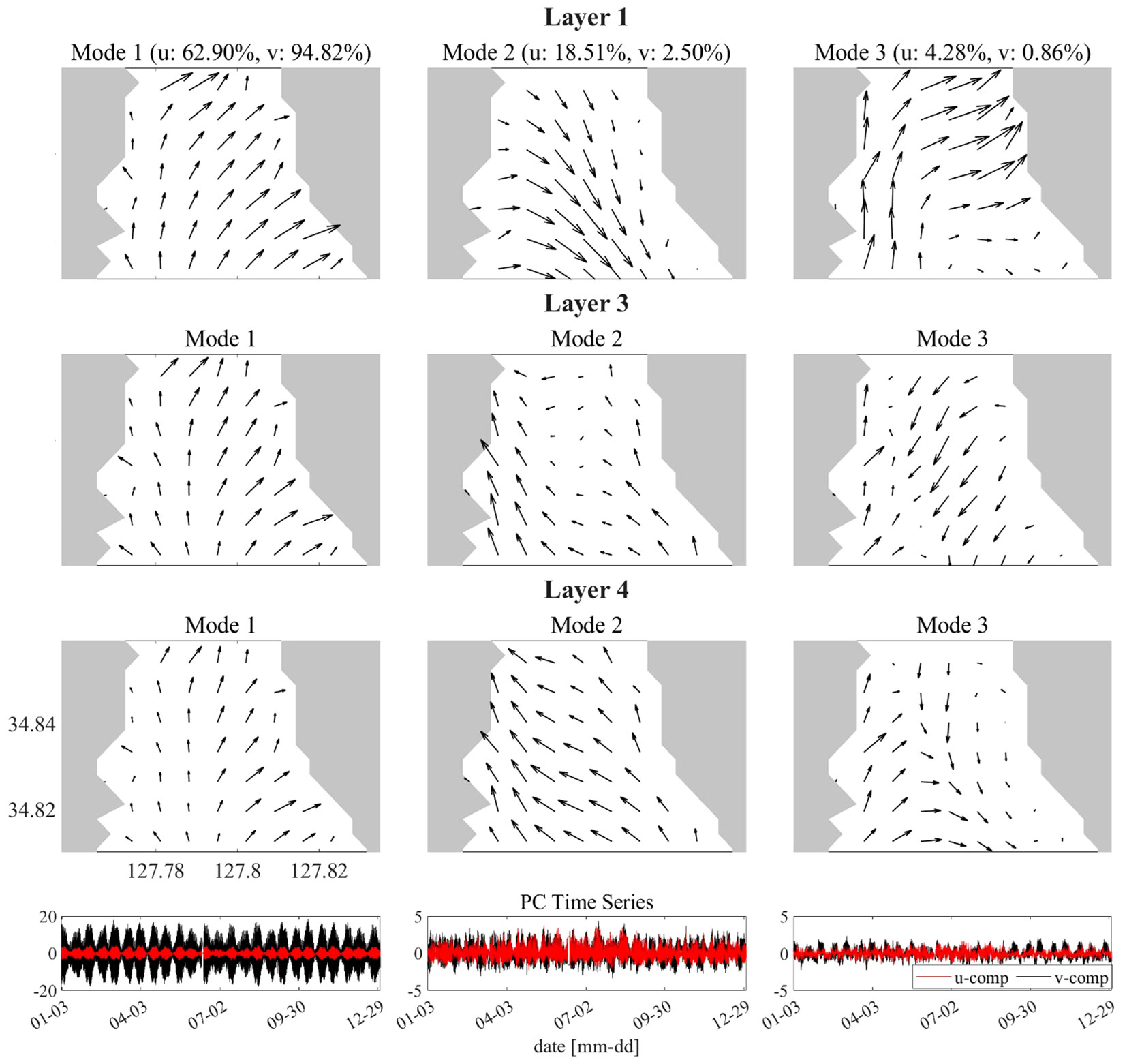
Figure 2 Three-dimensional EOF analysis results. (Rows) Eigenvectors for the first 3 modes (columns from left to right) at Layers 1, 3, and 4 (top three rows). Bottom panels represent time series of the principal components for the first 3 modes for u- (red) and v-components (black).

Figure 2 shows the eigenvector field and PC time series for the first three modes with significant patterns obtained from EOF analysis. The results are presented for layers 1, 3, and 4, representing the upper, middle, and lower layers, respectively. This is characterized by the dominance of north-south reciprocating components in mode 1. The first five modes were used in the ‘E matrix’ of inverse analysis. The five modes explained 90.73% and 98.80% of the u- and v-component variance, respectively. The eigenvectors of the five modes are extracted for each transmission path and layer. Using the extracted vectors, ‘E matrix’ was defined as follows:

$${\mathit{\text{E}}}_{\mathit{\text{ijk}}}=\frac{\mathbf{2}}{{\mathit{\text{C}}}_{\mathbf{0}}^{\mathbf{2}}}{\int }_{\mathbf{0}}^{{\mathbf{R}}_{\mathit{i}}}{\mathit{\text{u}}}_{\mathit{\text{jk}}}\mathit{\text{cos}}{\mathit{\theta }}_{\mathit{\text{i}}}+{\mathit{\text{v}}}_{\mathit{\text{jk}}}\mathit{\text{sin}}{\mathit{\theta }}_{\mathit{\text{i}}} \mathit{\text{ds}}$$

where, i, j and k are the paths, modes, and layers, respectively; R_i is the length of each path; and C₀ is the reference sound speed. θ_i is the angle between each transmission path and the x-axis. Then, E_ijk, Y_ik, the unknown matrix X, and error e have the following relationships:

$$\mathit{Y}=\mathit{E}\mathit{X}+\mathit{e}$$

Applying the L-curve method to this relationship yields the point at which error(e) and solution(X) are optimally balanced (Hansen and O’Leary, 1993; Park and Kaneko, 2001). This inverse analysis for layer 1 (k=1, skipped notation) can be expressed as the following matrix: When this is performed for all five layers, we obtain the X matrix (j*k), which is dot-produced with the eigenvectors to yield a 3-D current field (U_k, V_k) by summing over each mode, as follows:

$${\mathit{\text{X}}}_{\mathit{\text{kj}}}=\left[\begin{array}{c}\begin{array}{cc}{\mathit{\text{a}}}_{\mathbf{11}}\mathbf{\cdots }{\mathit{\text{a}}}_{\mathbf{1}\mathit{\text{j}}}& {\mathit{\text{b}}}_{\mathbf{11}}\mathbf{\cdots }{\mathit{\text{b}}}_{\mathbf{1}\mathit{\text{j}}}\\ {\mathit{\text{a}}}_{\mathbf{21}}\mathbf{\cdots }{\mathit{\text{a}}}_{\mathbf{2}\mathit{\text{j}}}& {\mathit{\text{b}}}_{\mathbf{21}}\mathbf{\cdots }{\mathit{\text{b}}}_{\mathbf{2}\mathit{\text{j}}}\end{array}\\ \begin{array}{cc}\mathbf{⋮}\mathbf{⋮}& \mathbf{⋮}\mathbf{⋮}\\ {\mathit{\text{a}}}_{\mathit{\text{k}}\mathbf{1}}\mathbf{\cdots }{\mathit{\text{a}}}_{\mathit{\text{kj}}}& {\mathit{\text{b}}}_{\mathit{\text{k}}\mathbf{1}}\mathbf{\cdots }{\mathit{\text{b}}}_{\mathit{\text{kj}}}\end{array}\end{array}\right] ,$$

$$U_k=u_{k1}{a}_{k1}+u_{k2}{a}_{k2}+ \cdots +u_{kj}{a}_{kj}, and V_k=v_{k1}{b}_{k1}+v_{k2}{b}_{k2}+ \cdots +v_{kj}{b}_{kj}.$$

3 Results

3.1 Validation of along-path current of KOOS

First, we validated the KOOS model output data used in this study. The shipboard ADCP data observed along the paths between two stations in the domain were used. The shipboard ADCP observation period and the number of transection observations for each path are listed in Table 3. Observations were conducted during both the spring and neap tidal periods. Comparisons of the along-path-averaged velocities between the observations and the KOOS outputs showed highly correlated features, as shown in Figure 3. The RMSE values were 0.09, 0.12, 0.07 m/s, correlation coefficient (R) values were 0.88, 0.78, and 0.95, and p-values were 0.00, 0.01, 0.05 for S2, S3, and S4, respectively. This confirmed that the current field reproduced by the KOOS model was suitable for this study.

Table 3

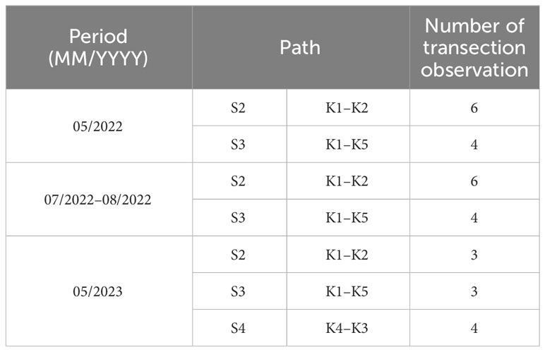
Table 3 Summary of shipboard ADCP observations.

Figure 3

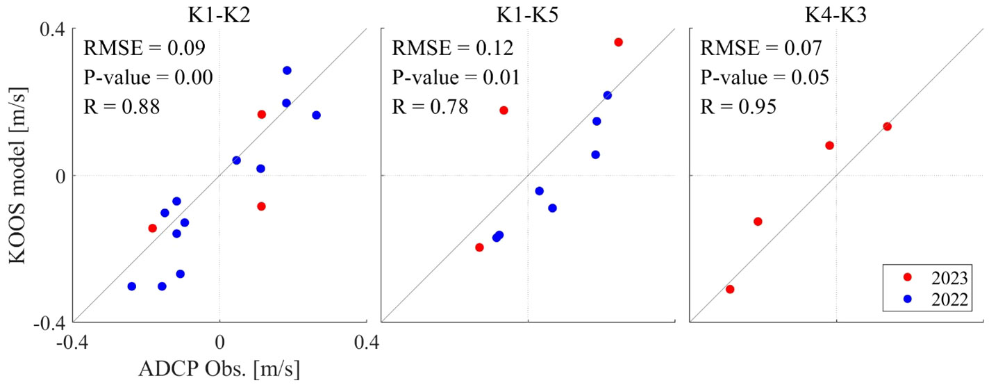
Figure 3 Comparison of along-path averaged velocity between ADCP observations and KOOS model outputs. Blue and red dots indicate ADCP observations carried out in 2022 and 2023, respectively. RMSE, R (correlation coefficient) values, and p-values are calculated for the entire period.

3.2 Validation for three-dimensional current field estimation

3.2.1 Validation for the along-path current velocity

The method presented in Section 2.2 was applied to all five horizontal layers in the domain, resulting in a 3-D current field. The estimated current field was validated by comparison with KOOS outputs. Owing to the characteristics of CAT, sound waves propagating along a path are significantly affected by the along-path current velocity. For this reason, current velocity was converted to the along-path current velocity (u cosθ + v sinθ), which is used in validation. Therefore, S1 (K1–K3) and S6 (K4–K5), which are nearly zonal to the latitude line, were slightly influenced by the north-south components of the current.

Figure 4 shows a comparison between the KOOS and estimated current fields for the along-path current velocity on S4 (K4–K3). Each figure compares the true values with the inverse estimation results using scatter plots and time-series plots. The results are shown for layers 1, 3, and 4 to present the characteristics of the current fields in the upper, middle, and lower layers, respectively. The estimated current field successfully reproduced the tidal variations, including the flood-ebb and spring-neap cycles, for the current velocity of the true values. Table 4 summarizes the average RMSE and R for all six paths and layers 1, 3, and 4. The estimated current field reproduced the KOOS current fields for all paths well, with average RMSE values less than 4 cm/s and average R values exceeding 0.9.

Figure 4

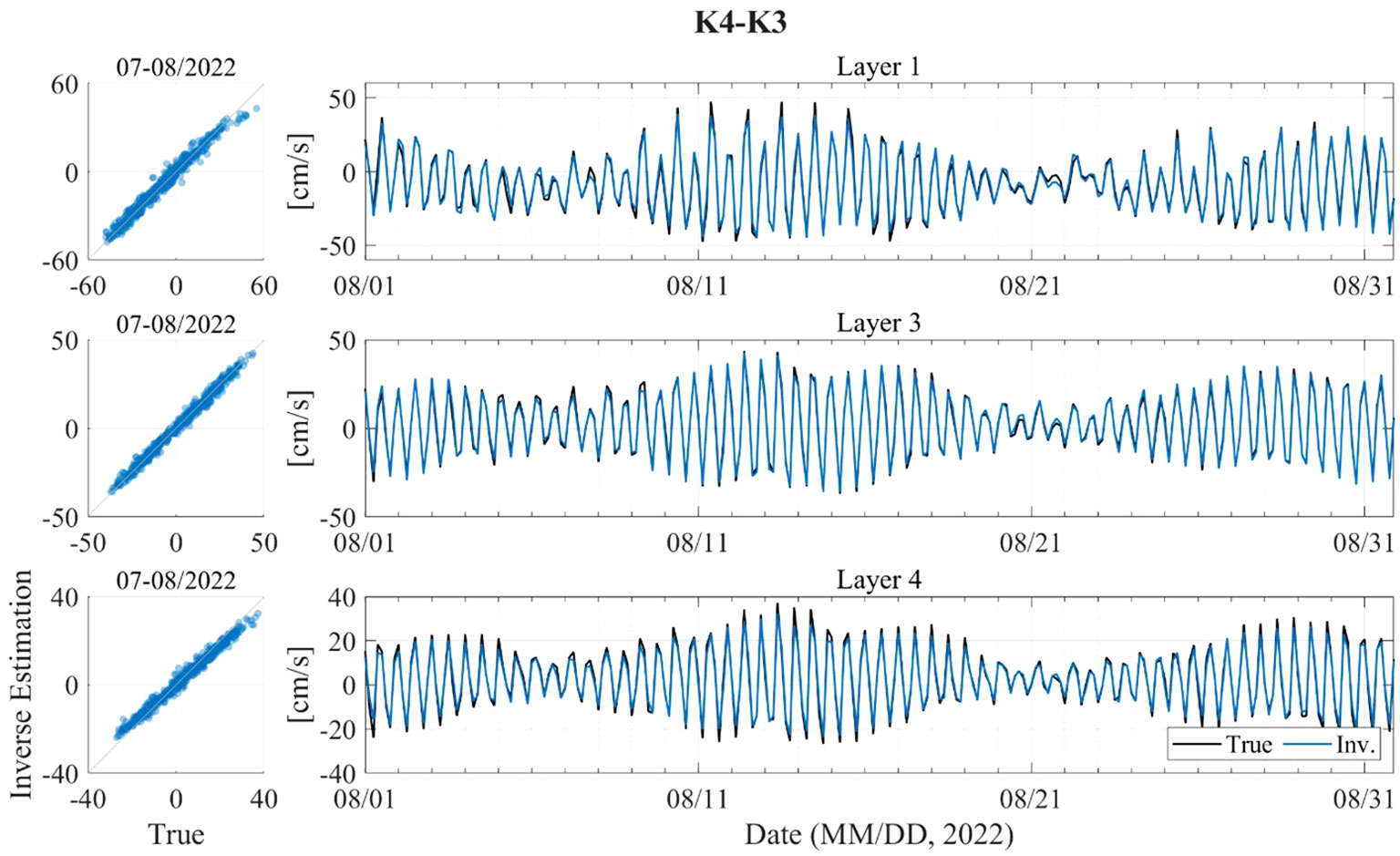
Figure 4 Comparison between the true value (KOOS model outputs, black) and results from the inverse estimation (blue) on S4 (K4–K3).

Table 4

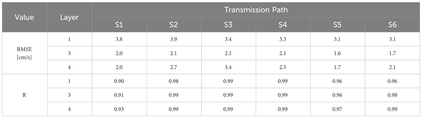
Table 4 RMSE (unit: cm/s) and R (correlation coefficient) values between the true current fields (KOOS model outputs) and inverse estimations.

3.2.2 Vertical and horizontal current fields

Yeosu Bay is dominated by the v-component, and the upper and lower layers sometimes exhibit opposite phases, depending on the tidal phase. This can be observed from snapshots of v-component along the section, which are presented in Figure 5. When comparing the true values in the first column with the estimated current fields in the second column, the two-layer structure is reproduced similarly in the contours in the first row. In addition, the flood tidal period-averaged contours show a northward flow in all five layers, and the ebb tidal period-averaged contours show a southward flow, which is very similar between the estimated and true values. The difference (True - estimation) is higher than -3.8 cm/s and lower than 3.2 cm/s. For the other paths, snapshots are not presented because they show patterns like those of S1 (K1–K3).

Figure 5

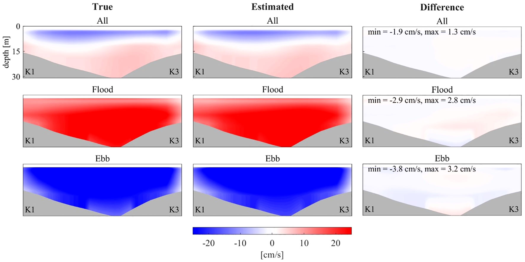
Figure 5 V-component along the section between K1 and K3 averaged (top panels) during July–August 2022, (middle panels) during the flood tidal period, and (bottom panels) during the ebb tidal period. First and second columns represent the true current field from the KOOS model and the results from the inverse estimation, respectively. Third column represents the difference between them (True - Estimation). Gray-shading indicates the sea floor.

Figure 6 shows snapshots of the vector representations of the horizontal current field in each layer. Both the southward and northward current periods produced current fields with low errors across the domain (Figure 6). In addition, the two-layer structure with a southward (northward) current in the upper (lower) layer was reproduced well (Figure 6). Figures 5, 6 present the validation results for the summer season (July and August 2022) when stratification is pronounced and the current structure is relatively complex.

Figure 6

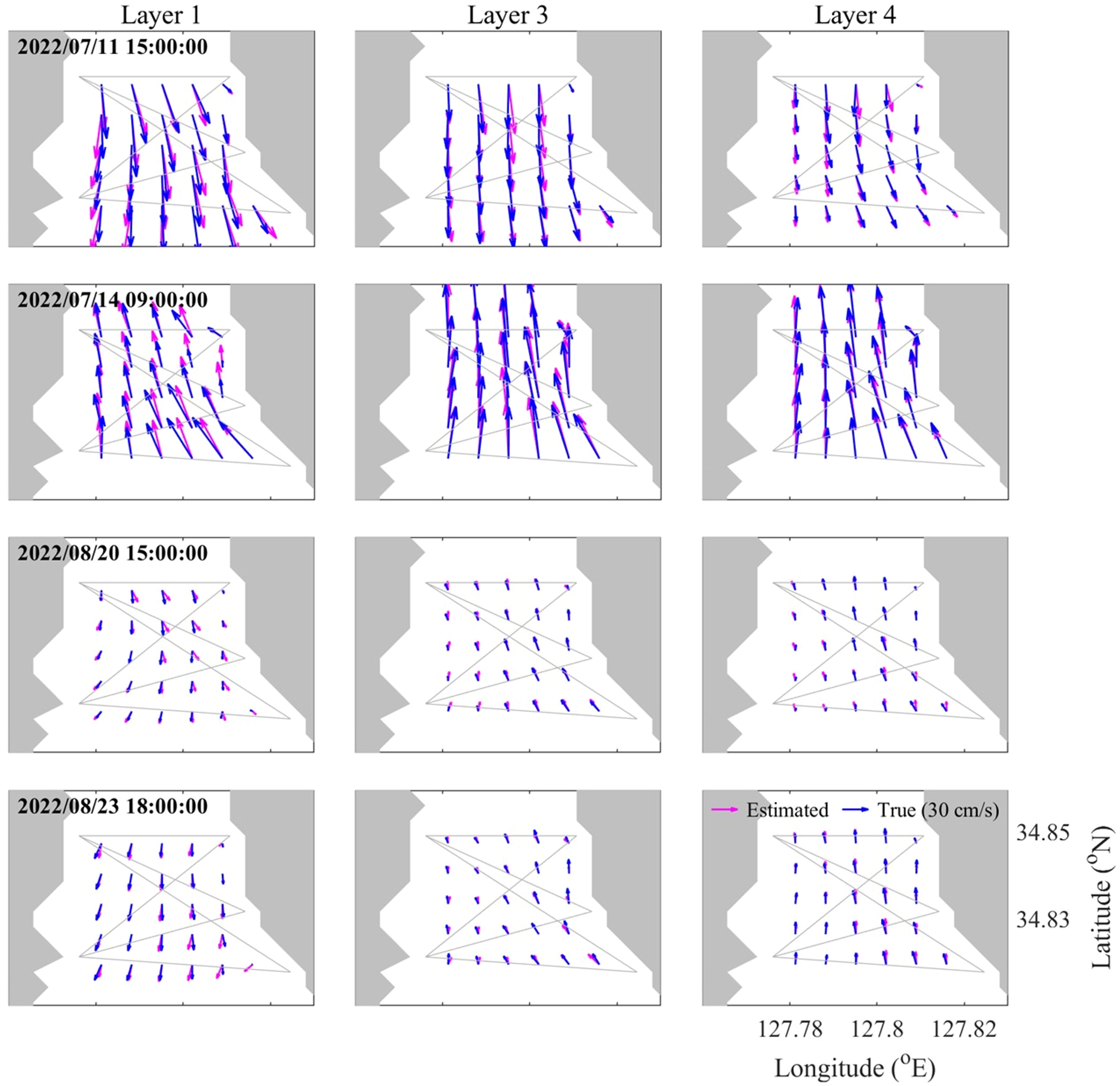
Figure 6 Snapshots of mapped current velocity at Layers 1, 3, and 4. Magenta and blue arrows indicate the results from the inverse estimation and the true value from KOOS model, respectively.

4 Discussion

4.1 RMSE and PVE of three-dimensional current fields

The RMSE fields of the estimated current for each layer during the validation period are shown in Figure 7. The spatially averaged RMSE values for each layer are indicated in parentheses. The error of the u-component is slightly lower than that of the v-component. The errors were somewhat higher in the upper layer than in the middle and bottom layers and were larger in areas where the simulation path did not intersect or at the edges of the domain.

Figure 7

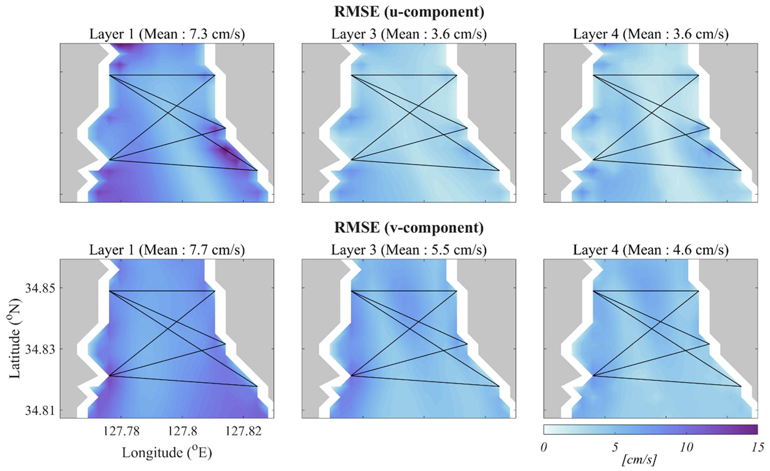
Figure 7 RMSE of u-component and v-component in January, February, July, and August 2022. Black lines indicate simulation paths, and gray-shaded parts are land.

The percent of variance explained (PVE) for each layer indicates the degree to which the estimated current field reproduces the variability compared to the true value. It is calculated using the equation ‘PVE = (1– σ_err²/σ_true²)*100’, where σ_true² and σ_err² represent the variance of the true value and the error (true value – calculated value), respectively. Figure 8 shows the PVE for each layer. The values in each title within the parentheses, expressed as percentages, represent the average PVE values within the domain enclosed by the six simulation paths. The average PVE for the u-component ranged from 49.8% to 68.9%, with approximately 10% variation among the layers. For the v-component, the average PVE ranges from 93.8% to 96.0%, with a variation of approximately 1% among the layers. This result suggests that the higher RMSE in the upper layer compared to the middle and bottom layers can be attributed to the higher current velocity values and variability in the upper layer. The higher PVE for the v-component compared to the u-component is interpreted to be caused by the EOF related to the domain characteristics represented by the simple current pattern in the v-component.

Figure 8

Figure 8 PVE of u-component and v-component in January, February, July, and August 2022. Black lines indicate simulation paths, and gray-shaded parts are land.

4.2 Noise test using the AI model

In contrast to ray-tracing simulations utilizing the Bellhop model, in-situ data may encompass a diverse array of noise. To assess the impact of noise within in-situ data on inverse analysis, a noise test was conducted, artificially introducing noise to the results (Δt) of the ray-tracing simulation. The noise was configured to follow a random normal distribution, and 11 experiments were structured based on varying noise intensities. The application of noise in each experiment is governed by the following equation:

$$\mathit{\Delta }{t}_{\mathit{\sigma }}=\mathit{\Delta }t+N(0,1)*\mathit{\sigma },\mathit{\sigma }=\mathit{\sigma }\text{'}*n$$

Here, n was established based on the maximum, minimum, and mean values derived from the observational results of CAT and the ray-tracing simulation results (Table 5). Table 6 lists the mean values of the RMSE for the along-path current calculated from the AI model noise test. The difference in RMSE between Case 1 (no noise) and Case 7 (noise with a magnitude of 10×σ’) was computed to be less than 1 cm/s. And RMSE difference between Case 1 and Case 11 (noise with a magnitude of 200×σ’) was calculated to be less than 4.4 cm/s. This implies that even with a 20-fold increase in the magnitude of noise, the increase in error was less than 2.2 times. Consequently, the AI model demonstrated the capability of reducing the noise inherent in the observational results of CAT. Therefore, these experiments suggest the feasibility of conducting quality control of CAT data using an AI model.

Table 5

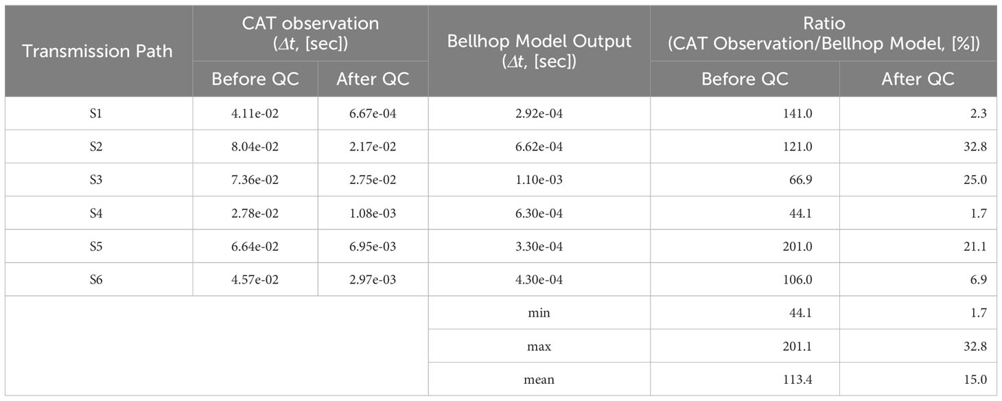
Table 5 CAT observation and Bellhop Model output data used for determining standard deviation (unit: sec, %).

Table 6

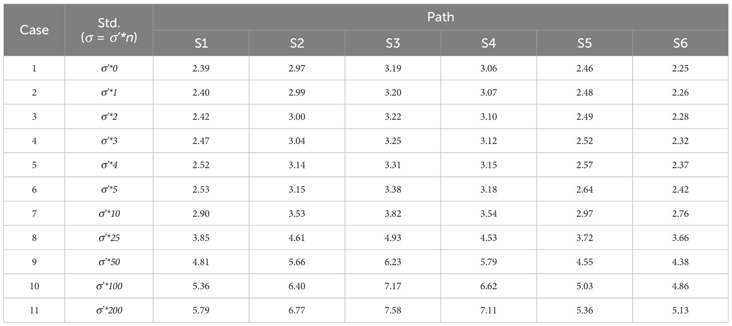
Table 6 RMSE of the along-path-averaged velocity between true value (KOOS model output) and the results from AI model noise test (unit: cm/s).

4.3 Application to in-situ CAT observation

The method in Section 2.2 is applied to in-situ CAT observation data using same method and data except for Δt. Here, the in-situ data were utilized instead of Bellhop outputs. The validation of the estimated current field using in-situ CAT data was performed by comparison with the ADCP mooring data. Each subplot is a scatter plot for each layer and the ADCP mooring site. Note that the station K1 was moved southward (34.8397°N, 127.7748°E) to obtain stable and high quality in-situ observation data. The map in Figure 9 is provided to indicate the relocated K1 station.

Figure 9

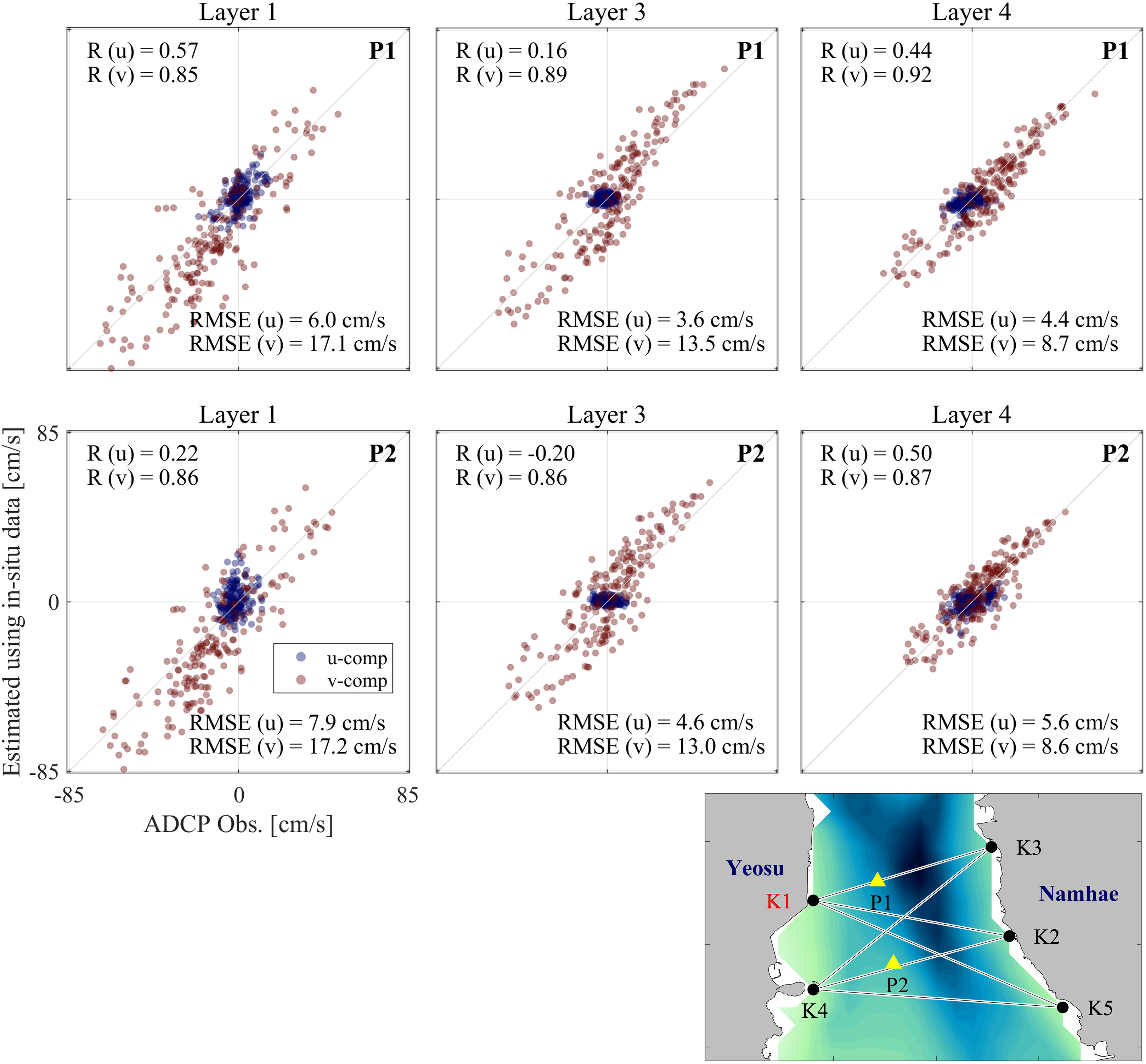
Figure 9 Scatter plots of currents between the observations from ADCP moorings and estimations from the inverse analysis using in-situ CAT data. Upper three panels are for mooring site P1 and lower three panels are for mooring site P2. Columns indicate Layers 1, 3, and 4 from left to right. Correlation coefficient (R) and RMSE values between the observed and estimated zonal and meridional (u and v) currents are shown in each panel. “Light blue and red dots indicate u- and v-components, respectively.”.

The v-component exhibited a lower RMSE and higher correlation coefficient than the u-component, which is attributed to the alignment of the current direction of the v-component with the along-channel direction. Upon examining the KOOS model as of September and October 2022, it was observed that the v-component had a minimum of 3.8 times and a maximum of 9.9 times higher standard deviation in the five layers than the u-component at the nearest grid to P1 and P2, respectively. In contrast, the observed currents at P1 and P2 showed a standard deviation of at least 2.3 times and up to 6.1 times higher for the v-component than for the u-component in the five layers. This indicates a significant deviation between the two components of the current velocity in the KOOS model used to develop the proposed method in this study. These characteristics of the KOOS model output and its spatial resolution of 300 m appear to account for the differences between the components in the validation results. This issue may be addressed in a future study by improving our 3-D current field inverse method by utilizing a high-resolution coastal ocean model with spatial and temporal resolutions of 100 m and 30 min, respectively.

5 Conclusion

In this paper, we propose a new method for estimating the three-dimensional current field by combining AI and inverse methods. Ray-tracing simulations were performed using the Bellhop model, and the range-averaged currents at five layers and six simulation paths were obtained from the AI model. The inverse method is applied to each of the five horizontal layers, resulting a 3-D current fields. The significance of this study can be summarized as follows:

First, the 3-D current field was estimated for the first time by combining AI and inverse methods. The CAT in-situ observations are theoretically capable of identifying rays passing through all layers, but this is challenging in practice, making it difficult to estimate current fields in the vertical sections of the experimental paths. An AI model was employed to obtain the current fields in the vertical sections. Furthermore, applying the EOF of the current fields to the inverse method simplified the coastal boundary condition problem by incorporating the current-field characteristics of the domain through the first five EOF modes.

Second, the noise test of the AI model showed that it can handle the noise generated by the observations; therefore, it is applicable to CAT in-situ observations, which are expected to contain more noisy signals than ray tracing simulations. In fact, after applying the AI model to CAT in-situ observations taken in the domain over a one-month period starting on September 22, 2023, the estimated current fields showed that the along-channel velocity matched well with the ADCP mooring data at the two points inside the domain (R > 0.85). These results suggest that our novel 3-D current field estimation method is applicable to in-situ CAT data in the Yeosu Bay. In addition, since the high-resolution KOOS model outputs are available all around the coastal seas of Korea, its application would be possible to other coastal areas where the CAT system is installed to continuously monitor 3-D current changes.

Data availability statement

The original contributions presented in the study are included in the article/Supplementary Material. Further inquiries can be directed to the corresponding author.

Author contributions

YH: Writing – original draft, Writing – review & editing, Conceptualization, Data curation, Formal analysis, Investigation, Methodology, Validation, Visualization. EL: Data curation, Methodology, Validation, Visualization, Writing – original draft, Writing – review & editing. HS: Data curation, Formal analysis, Writing – review & editing. B-NK: Data curation, Investigation, Writing – review & editing. HH: Data curation, Investigation, Writing – review & editing. YC: Data curation, Investigation, Writing – review & editing. JK: Data curation, Writing – review & editing. JP: Writing – original draft, Writing – review & editing, Conceptualization, Funding acquisition, Methodology, Project administration, Supervision.

Funding

The author(s) declare financial support was received for the research, authorship, and/or publication of this article. This research was funded by the Ministry of Oceans and Fisheries, Korea (grant number 20210642, “Development of 3-D Ocean Current Observation Technology for Efficient Response to Maritime Distress”).

Conflict of interest

The authors declare that the research was conducted in the absence of any commercial or financial relationships that could be construed as a potential conflict of interest.

Publisher’s note

All claims expressed in this article are solely those of the authors and do not necessarily represent those of their affiliated organizations, or those of the publisher, the editors and the reviewers. Any product that may be evaluated in this article, or claim that may be made by its manufacturer, is not guaranteed or endorsed by the publisher.

Supplementary material

The Supplementary Material for this article can be found online at: https://www.frontiersin.org/articles/10.3389/fmars.2024.1362335/full#supplementary-material

References

Chen M., Zhu Z. N., Zhang C., Zhu X. H., Wang M., Fan X., et al. (2020). Mapping current fields in a bay using a coast-fitting tomographic inversion. Sensors 20, 558. doi: 10.3390/s20020558

PubMed Abstract | CrossRef Full Text | Google Scholar

Del Grosso V. A. (1974). New equation for the speed of sound in natural waters (with comparisons to other equations). J. Acoustical Soc. America 56, 1084–1091. doi: 10.1121/1.1903388

CrossRef Full Text | Google Scholar

Hansen P. C., O’Leary D. P. (1993). The use of the L-curve in the regularization of discrete ill-posed problems. SIAM J. Sci. Comput. 14, 1487–1503. doi: 10.1137/0914086

CrossRef Full Text | Google Scholar

Kaneko A., Zhu X. H., Lin J. (2020). Coastal acoustic tomography (Amsterdam, Netherlands: Elsevier). doi: 10.1016/B978-0-12-818507-0.00014-7

CrossRef Full Text | Google Scholar

Lee J. C., Kim J. C. (2007). Current structure and variability in Gwangyang Bay in spring 2006. The Sea: Journal of the korean society of oceanography. 12 (3), 219–224. Available at: http://uci.or.kr/G704-000255.2007.12.3.016.

Google Scholar

Munk W., Wunsch C. (1979). Ocean acoustic tomography: A scheme for large scale monitoring. Deep Sea Res. Part A. Oceanogr. Res. Papers 26, 123–161. doi: 10.1016/0198-0149(79)90073-6

CrossRef Full Text | Google Scholar

Park J. H., Kaneko A. (2000). Assimilation of coastal acoustic tomography data into a barotropic ocean model. Geophys. Res. Lett. 27, 3373–3376. doi: 10.1029/2000GL011600

CrossRef Full Text | Google Scholar

Park J. H., Kaneko A. (2001). Computer simulation of coastal acoustic tomography by a two-dimensional vortex model. J. Oceanogr. 57, 593–602. doi: 10.1023/A:1021211820885

CrossRef Full Text | Google Scholar

Porter M. B. (2011). The bellhop manual and user’s guide: Preliminary draft Vol. 260 (La Jolla, CA, USA: Heat, Light, and Sound Research, Inc.). Tech. Rep.

Google Scholar

Pritchard D. W. (1952). Salinity distribution and circulation in the Chesapeake Bay estuarine system. J. Mar. Res. 11 (2), 106–123. Available at: https://elischolar.library.yale.edu/journal_of_marine_research/763.

Google Scholar

Yamoaka H., Kaneko A., Park J. H., Zheng H., Gohda N., Takano T., et al. (2002). Coastal acoustic tomography system and its field application. IEEE J. Oceanic Eng. 27, 283–295. doi: 10.1109/JOE.2002.1002483

CrossRef Full Text | Google Scholar

Zhang C., Zhu X. H., Zhu Z. N., Liu W., Zhang Z., Fan X., et al. (2017). High-precision measurement of tidal current structures using coastal acoustic tomography. Estuar. Coast. Shelf Sci. 193, 12–24. doi: 10.1016/j.ecss.2017.05.014

CrossRef Full Text | Google Scholar

Zhu X. H., Kaneko A., Wu Q., Zhang C., Taniguchi N., Gohda N. (2012). Mapping tidal current structures in Zhitouyang Bay, China, using coastal acoustic tomography. IEEE J. Oceanic Eng. 38, 285–296. doi: 10.1109/JOE.2012.2223911

CrossRef Full Text | Google Scholar

Zhu Z. N., Zhu X. H., Guo X., Fan X., Zhang C. (2017). Assimilation of coastal acoustic tomography data using an unstructured triangular grid ocean model for water with complex coastlines and islands. J. Geophys. Res.: Oceans 122, 7013–7030. doi: 10.1002/2017JC012715

CrossRef Full Text | Google Scholar

Zhu Z. N., Zhu X. H., Zhang C., Chen M., Wang M., Dong M., et al. (2021). Dynamics of tidal and residual currents based on coastal acoustic tomography assimilated data obtained in Jiaozhou Bay, China. J. Geophys. Res.: Oceans 126, e2020JC017003. doi: 10.1029/2020JC017003

CrossRef Full Text | Google Scholar