 Scott N. Evans
 Nick Konzewitsch
 Renae K. Hovey
 Gary A. Kendrick
 Lynda M. Bellchambers1
- 1Western Australian Fisheries and Marine Research Laboratories, Department of Primary Industries and Regional Development, Government of Western Australia, Perth, WA, Australia
- 2School of Biological Sciences and University of Western Australia (UWA) Oceans Institute, University of Western Australia, Perth, WA, Australia
A spatially explicit understanding of marine benthic habitats is essential for sustainable marine resource management. While advances in remote sensing, acoustic methodologies, geostatistical modelling, and predictive species distribution models have improved our ability to map underwater habitats, selecting the most appropriate approach, particularly in turbid or remote regions, remains challenging. This study was conducted in the protected nursery area of the Exmouth Gulf Prawn Managed Fishery in Western Australia and compared four commonly used “off-the-shelf” mapping techniques. These included satellite remote sensing, acoustic sounding, predictive modelling, and geostatistical interpolation, with each technique evaluated using comprehensive ground-truthing and output confidence matrices. Geostatistical kriging emerged as the most robust method, delivering the highest predictive accuracy, quantifiable confidence, and spatially explicit seasonal habitat maps. These maps delineated submerged aquatic vegetation, including seagrass and macroalgae, at broad spatial scales and captured seasonal shifts in habitat distribution and density. Our findings enhance knowledge of benthic habitats in Exmouth Gulf and underscore that effective marine habitat mapping, particularly in dynamic and turbid environments, cannot rely on remote methods alone. Spatially balanced field data collection at ecologically relevant temporal scales is essential to support sustainable marine resource management.
1 Introduction
In the last decade fisheries management globally has undergone a shift from a target species approach to the more holistic ecosystem based fisheries management (EBFM) that considers the broader ecosystem (Townsend et al., 2019). A key component of EBFM is a spatially explicit understanding of marine benthic habitats, their productivity and relationship with commercially important species (Overly and Lecours, 2024). A lack of comprehensive data on the distribution and abundance of habitat types and their role as essential fish habitats results in knowledge gaps that may limit scientific advice and effective decision making for sustainable fisheries management and marine spatial planning (Moore et al., 2016).
With marine habitats under increasing pressure, from climate change (Abdo et al., 2012; Hickey et al., 2020; Strydom et al., 2020) and coastal development (Orth et al., 2006), there is urgent need to map and monitor habitats to support effective management for the sustainable use of aquatic resources and marine conservation (Brown and Collier, 2008; Cogan et al., 2009; Ware and Downie, 2020; Arenas-Castro and Sillero, 2021). Benthic habitat maps can be used to monitor changes in habitat distribution and condition over time, to assess the effectiveness of management actions and identify emerging threats (Menandro et al., 2022). However, producing habitat maps for large or complex marine environments often remains a challenge due to the submerged nature of these environments and the associated difficulty of data collection (Mumby et al., 2001; Madin and Madin, 2015).
Advances in technology, particularly in remote sensing, acoustic methodologies and geostatistical modelling, have enhanced our ability to map marine habitats (Brown et al., 2011; Smith Menandro and Cardoso Bastos, 2020; McKenzie et al., 2022; Mastrantonis et al., 2024b; Misiuk and Brown, 2024). However, challenges remain to ensure there is an appropriate level of spatial and temporal detail in field data and maps, with the statistical confidence required to inform EBFM (Schultz et al., 2015; Moore et al., 2016; Roelfsema et al., 2020; Ware and Downie, 2020; McKenzie et al., 2022; Mastrantonis et al., 2024b). These challenges often relate less to technical limitations and more to selecting the most suitable approach. While many studies rely on a single approach, due to resource constraints or user preference, greater use of preliminary comparative assessments of techniques tailored to specific fisheries or management areas may reduce the uncertainty of outputs and improve decision making (Lecours, 2017; Bastardie et al., 2021).
Satellite remote sensing, acoustic sounding, geostatistical (interpolation) modelling and predictive modelling are four common marine habitat mapping tools. Satellite remote sensing has a long history in marine habitat mapping. However, remote sensing in aquatic environments can be complex due to water properties such as depth and turbidity (Dahdouh-Guebas, 2002; Franklin, 2010) as well as the presence of diverse habitat types within the resolution of a single pixel (Mastrantonis et al., 2024b). Therefore, validation of unsupervised satellite classifications is essential (Lu and Weng, 2007; Schultz et al., 2015). Machine learning algorithms such as Support Vector Machine, Random Forest (RF), and Artificial Neural Networks (ANN), also enhance the accuracy and efficiency of classification by processing large datasets and extracting complex patterns (Wulder et al., 2022). Advancements in freely available high-resolution imagery and rapid resurvey capabilities make satellite remote sensing a cost-effective tool for managing nearshore habitats. However, its effective use requires outputs that are fit-for-purpose and limitations are assessed and communicated to allow for robust decision making.
Similarly, acoustic sounding (hydroacoustics) has been used to map the marine benthic environment for over five decades by using soundwaves to capture data on seabed features, particularly in deep or turbid environments, where optical methods are not well-suited (Misiuk and Brown, 2024). Recent advances have expanded the use of acoustic sounding to assess submerged aquatic vegetation (SAV), such as dense seagrass meadows and canopy forming macroalgae. However, the discrimination of low-canopy or sparsely distributed vegetation remains a challenge (Gumusay et al., 2019; Kruss et al., 2019).
Species distribution modelling (SDM) is widely used to map habitats in areas where full observational coverage is restricted by turbidity, depth, or remoteness (Robinson et al., 2017; Pickens et al., 2021). Geostatistical interpolation techniques, such as kriging, estimate environmental variables at unsampled locations using principles of spatial autocorrelation, while deterministic methods such as inverse distance weighting (IDW), spline, and natural neighbour, rely on spatial proximity (Shumchenia and King, 2010; Li and Heap, 2014). Kriging is particularly useful due to its ability to incorporate spatial relationships and provide uncertainty estimates (Krige, 1951; Wu & Hung, 2016), Spline interpolation suits variables with gradual spatial changes, and IDW offers simplicity and computational efficiency for homogenous distributions (Wu and Hung, 2016). Predictive machine learning techniques further expand SDM capabilities by modelling complex, non-linear relationships between species occurrences and environmental predictors (Melo-Merino et al., 2020; Misiuk and Brown, 2024). Methods like RF, Maximum Entropy (MaxEnt), ANN, and Boosting are useful in handling large datasets and imbalanced presence/absence data (Phillips et al., 2006; Franceschini et al., 2019; Norberg et al., 2019; Rubbens et al., 2023). Ultimately, the choice between geostatistical and machine learning methods depends on the data, ecological dynamics, and management objectives (Li and Heap, 2014).
Exmouth Gulf is an important marine embayment in Western Australia, valued for its social, ecological and economic significance (Fitzpatrick et al., 2019). However, its remoteness and highly turbid environment create challenges for the collection of benthic habitat information. Previous studies have focused on quantifying the abundance and distribution of broad habitat classes based on their occurrence at specific point locations (McCook et al., 1995; Loneragan et al., 2013; Vanderklift et al., 2016; Cartwright et al., 2023) or collecting discrete data to inform wider bioregional occurrence or genetic connectivity patterns, particularly for seagrasses (McMahon et al., 2017; Evans et al., 2021). However, habitat maps that provide a robust, spatially explicit understanding of the extent of habitat classes relevant to resource management are lacking. With high water turbidity (Cartwright et al., 2023) limiting the effectiveness of satellite-based optical methods, habitat maps produced for Exmouth Gulf have historically relied on different scales of ground truth data (e.g., UVC and tow video), collected at different time points, combined with geostatistical modelling (e.g., IDW, Krige) to estimate the spatial abundance and distribution of habitats (Loneragan et al., 2003; MBS, 2018; DPIRD, 2020). However, these maps have not incorporated confidence statistics, for model development and validation, likely due to the challenges of collecting sufficient ground-truth samples in a remote location. Without confidence statistics, it is difficult to determine whether these methods are fit-for-purpose for the study area, or to evaluate their robustness to support evidence-based management decisions. The aim of this study was to evaluate the suitability of existing cost-effective habitat mapping techniques, focusing on the confidence of their outputs, to identify the best approach for providing a quantitative spatial description of benthic habitats in the Exmouth Gulf Prawn Managed Fishery (EGPMF) nursery area. This information is crucial for fisheries management decisions, particularly concerning EGPMF recruitment patterns (DPIRD, 2020; DPIRD, 2021), while also supporting broader marine resource management within Exmouth Gulf (Fitzpatrick et al., 2019; Sutton and Shaw, 2021).
2 Methods
To aid interpretation, key terms, acronyms and descriptions related to statistical model algorithms and performance metrics used in this study are summarised in Tables 1 and 2.
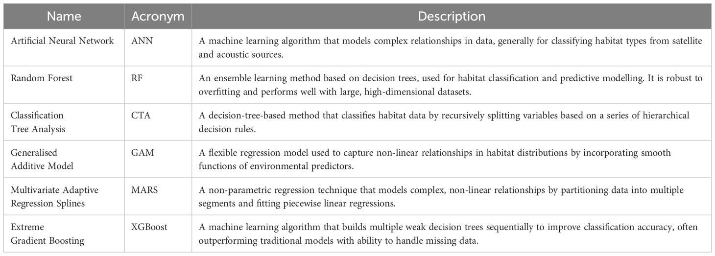
Table 1. Common habitat mapping algorithms.
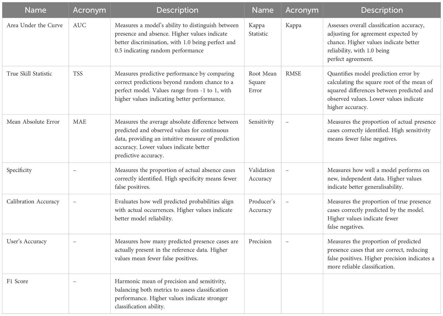
Table 2. Performance (confidence) metrics for model evaluation.
2.1 Study area
Located on the coast of Western Australia (22°0’S, 20'E), the EGPMF nursery area spans 1,139 km² (~29%) of Exmouth Gulf and has been closed to commercial prawn trawl fishing since the 1970’s (Figure 1) (DPIRD, 2020). Water depths are mostly <5m, gradually deepening to 15 m in the west (Figure 1). The area features fringing salt flats, cyanobacterial mats, mangroves and intertidal mudflats which transition into subtidal macroalgae flats, seagrass beds and sand or mud (McCook et al., 1995; Loneragan et al., 2013; DPIRD, 2021). High turbidity is a defining characteristic of Exmouth Gulf, driven by local factors like winds and tides, along with larger-scale oceanographic influences such as ENSO and the Indian Ocean Dipole (Cartwright et al., 2021).
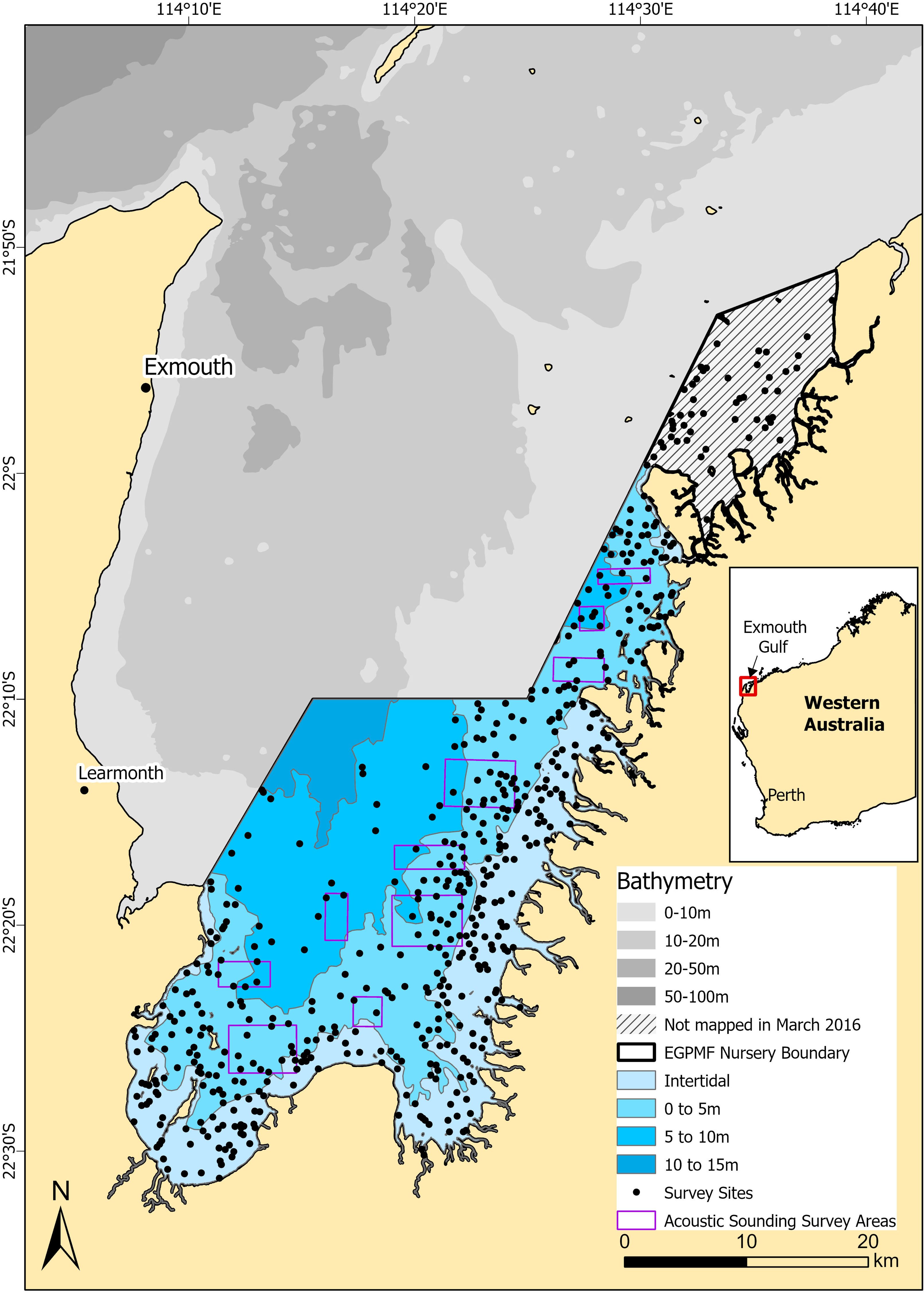
Figure 1. Map of Exmouth Gulf and the Exmouth Gulf Prawn Managed Fishery Nursery Area survey sites.
Exmouth Gulf receives occasional freshwater and associated nutrient inputs, mostly associated with summer tropical low-pressure systems and run off from Cape Range to the west or the eastern arid plains (Lovelock et al., 2011; Fitzpatrick et al., 2019). These sporadic freshwater pulses and high evaporation rates result in inverse estuarine conditions, where salinity is generally highest on the landward edge (Tomczak and Godfrey, 2003; Fitzpatrick et al., 2019). Environmental patterns are characterised by high summer air temperature (mean maximum of 38°C in January), low rainfall (~260 mm/year), high evaporation rates (1700 mm to 3050 mm per annum) and mixed semi-diurnal tides with a maximum range of 3m (Semeniuk, 1985; Fitzpatrick et al., 2019; Australian Bureau of Meteorology, 2022).
2.2 Ground truth habitat data surveys – in water data collection
Ground truthing sites were selected by stratifying the study area into four depth zones: intertidal, 0–5 m, 5–10 m, and 10–15 m (Figure 1), using digitised bathymetry data from the Australian Hydrographic Services (2014). An unsupervised ten-class ISO cluster classification (Jain et al., 1999) was applied to the intertidal and 0–5 m depth zones using ESRI ArcGIS v10.3 Spatial Analyst extension (ESRI, 2011). The 5–10 m and 10–15 m depth zones were excluded from the unsupervised classification due to poor visibility beyond ~5 m in the imagery, which was derived from a single, cloud-free SPOT 6 satellite image (November 4, 2014) during neap high tide and low wind conditions (<15 knots) (Australian Bureau of Meteorology, 2022). Four hundred potential survey sites were then randomly stratified across the intertidal (200 sites) and 0–5 m (200 sites) depth zones, weighted by spatial area of each of the unsupervised ISO cluster classes, with a buffer of 200 m from the edge. Fifty sites were then randomly allocated in the 5–10 m depth zone and 62 sites placed throughout the study area based on local knowledge, resulting in 512 potential sites for the summer 2016 survey. No sites were selected in the 10–15 m depth range as it was expected to lack suitable prawn recruitment habitats. For the winter 2016 survey, 100 additional sites were added to the previously unmapped northern extent of the study area, bringing the total to 612 potential sites (Figure 1).
Surveys were conducted using a tethered drop video system comprised of a georeferenced, live feed GoPro Hero3/3+ camera (wide view, 16:9 aspect ratio, 1080p) mounted on a drop lander system to capture benthic imagery with a 0.2 m2 footprint per drop. The system captured benthic imagery approximately every 5 m along a 50 m transect, for a total of ten static frames per site (2 m2 per site). Surveys took place over two-week periods in March/April (‘summer’) and August/September (‘winter’) 2016, with 455 sites sampled in summer and 539 in winter, ensuring at least three sites per class, per depth range. Habitat images were analysed using Transect Measure© and the CATAMI classification scheme on a 64-point stratified grid, yielding 640 annotated points per site (Althaus et al., 2015; Hill et al., 2018). Mean habitat percentages were calculated, square root transformed and subjected to CLUSTER analysis with SIMPROF (significance level of 1%), in PRIMER v7©. This resulted in five statistically (p<0.05) distinct habitat classes: macroalgae, seagrass, zoanthids, unconsolidated substrate and ‘other’. All vegetated classes were also grouped into a submerged aquatic vegetation (SAV) class, with habitats classified as presence/absence and percent density. These 2016 ground truth habitat datasets represent the most extensive habitat data known to be available for the EGPMF nursery area and provide a baseline and foundation for evaluating habitat classification techniques.
2.3 Habitat mapping techniques - remote sensing
Supervised classification techniques were applied to Landsat-8 (https://www.usgs.gov/landsat-missions/landsat-8) and Sentinel-2 (https://scihub.copernicus.eu/) satellite images for summer (March/April) and winter (August/September) 2016. Selected satellite image scenes were cloud-free and the study area was fully captured within one scene (Table 3).
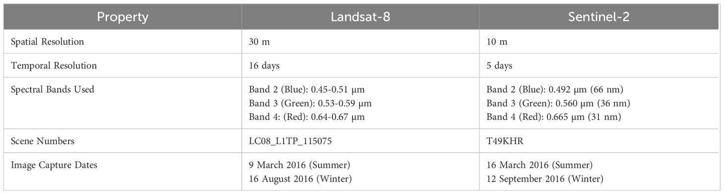
Table 3. Key properties of Landsat-8 and Sentinel-2 satellites used in this study.
Classification focused on mapping SAV presence/absence using ≥10% and ≥25% cover thresholds derived from the 2016 ground-truth datasets. A six-class habitat model was also developed for winter 2016 presence/absence dataset, with classes defined by the dominant vegetated habitat type. The six classes were: seagrass, macroalgae, dominant seagrass with macroalgae, dominant macroalgae with seagrass, sand (100% cover), and ‘SAV other’. Datasets were converted into point feature shapefiles in ArcGIS Pro v2.9 (ESRI, 2023), with a 50m buffer applied to represent transect length.
Image pre-processing for both sensors included atmospheric correction through QGIS using ESA SNAP (Sen2Cor plugin) (Main-Knorn et al., 2017; QGIS Development Team, 2020), clipping to the study area, projection to WGS 84 UTM Zone 50S and the exclusion of artefact-prone bands (e.g., Sentinel-2’s Coastal/Aerosol band). Only blue, green, and red bands were used, as the near-infrared and shortwave infrared were ineffective due to poor water penetration. Sun glint correction was tested on summer Sentinel-2 scene but excluded due to overcorrection issues and no improvement in accuracy.
Classification was conducted in SAGA GIS (v7.5), an open-source system for geospatial analysis and batch processing (Conrad et al., 2015), initially testing multiple algorithms (e.g., Boosted Classification, RF, ANN) on the Landsat-8 summer scene using the ≥25% threshold SAV presence/absence ground-truth dataset. The ANN achieved the highest kappa (0.48) and was used for final classifications on both sensors for both seasons. This involved randomly selecting 80% of ground-truth sites within the ≥10% and ≥25% SAV presence/absence thresholds and six-class datasets for training, with results exported as GeoTIFFs and vectorised as ArcGIS shapefiles. Validation with the remaining 20% of ground-truth sites was tested in the ORFEO Toolbox (Grizonnet et al., 2017) to generate confusion matrices.
2.4 Habitat mapping techniques – acoustic sounding
Acoustic data were collected using a Kongsberg EA400 SBES with a Simrad 38/200 Combi D transducer (38 kHz and 200 kHz) and Hemisphere R131 Differential-GPS. The transducer was mounted on a shallow-draft research vessel away from propeller wash. The SBES was chosen for its “off the shelf” availability, cost-effectiveness, ease of use, and suitability for the shallow study area, given the limited swath coverage of multi-beam echosounders (Gumusay et al., 2019). Surveys were conducted across 10 sites (3–20 km²) over eight days (1st-31st August 2017), focusing on areas ≥2 m deep and likely to contain SAV (Loneragan et al., 2003) (Figure 1). Parallel transects (~250 m apart) were surveyed at 5–6 knots in calm conditions (sea state <0.5 m, wind <12 knots). Data collection parameters included a 1 s−¹ ping rate, 1000W power, and a 0.256 ms pulse length. Water temperature, salinity and pH were measured to calibrate sound speed and absorption coefficients. Depth settings exceeded 2.5 times the maximum study area depth to ensure second echo acquisition.
Data processing in Echoview® v8 used the habitat classification module (Echoview, 2023a), which can extract nine acoustic features (Echoview, 2023b). Gaps in bottom detection were smoothed with a three-sample mean filter and manually validated. Data outside transect lines (e.g., vessel turns) were removed and the feature extraction interval was set to 30 m, aligning with comparable satellite imagery resolution. Principal components analysis indicated depth was not a dominant feature and was excluded to avoid bias. Dominant features, including first bottom length, skewness, and kurtosis, contributed ~50% of variation in PC1. The Calinski-Harabasz criterion was used to select the number of habitat classes by identifying the grouping that showed the clearest separation between classes. Unsupervised classifications were applied to two bottom echo thresholds (-100 dB and -110 dB) for each frequency, resulting in four acoustic classified datasets.
Geospatial analysis of the four classified datasets (-100db/38 kHz, -110db/38 kHz, -100db/200 kHz, -110db/200 kHz) was conducted using indicator kriging interpolation in R (v4.2.1) (Pebesma, 2004; R Core Team, 2023). Data were projected to UTM WGS84 Zone 50S with 80% used for training and 20% for testing accuracy. Variograms were modelled using an exponential approach (Gräler et al., 2016), and kriging predicted the most probable class for each location. Outputs were saved as GeoTIFF for visualisation and the documentation of performance metrics followed Kuhn (2008). To evaluate acoustic classes against habitat data, the winter 2016 ground-truth dataset (categorised as seagrass, macroalgae, and unconsolidated substrate) was used. Habitat occurrence was based on a ≥20% cover threshold. This dataset was overlaid on the acoustic rasters to analyse spatial correlations.
2.5 Habitat mapping techniques – predictive modelling
Predictive habitat modelling was conducted using the BIOMOD2 package (Thuiller et al., 2023) in R v4.2.1 (R Core Team, 2023), with 2016 summer (n=455) and winter (n=539) habitat datasets. Models evaluated macroalgae, seagrass, and combined SAV, the primary benthic habitats in the study area, defining presence/absence using a ≥20% cover threshold to ensure functional accuracy and avoid overfitting observed with lower thresholds. The only spatially comprehensive environmental predictor available for use at a comparable resolution was a 10 m resolution satellite-derived bathymetry (SDB) (Lebrec et al., 2021). Six modelling algorithms were initially tested: GAM, XGBoost, CTA, MARS, RF and ANN (Table 1). A 10-fold cross-validation approach was used to ensure robustness, with 80% of data used for training and 20% for validation. Model performance was assessed using a range of metrics (e.g., Table 2).
GAM, CTA, and MARS showed poor predictive performance and computational inefficiencies, leaving RF, XGBoost, and ANN for further evaluation. No single model excelled across all performance metrics (Table 4). However, RF was selected due to its balanced performance, lower risk of overfitting, and widespread use in habitat assessment. The low kappa values for RF (Table 4) are reflective of the presence/absence single predictor variable and imbalanced data in this study (dominated by unconsolidated substrate), with AUC and TSS likely a better indication of predictive reliability.
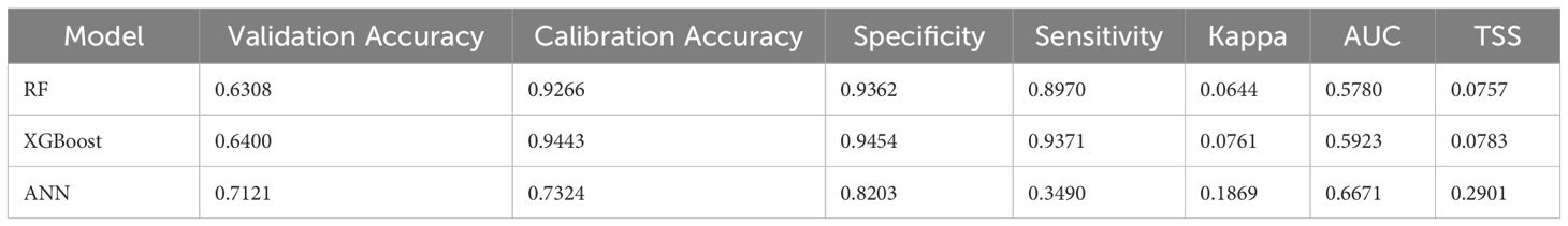
Table 4. Performance metrics geostatistical (Interpolation) modelling.
Individual predictive habitat maps for seagrass, macroalgae and SAV were generated using the R package randomForest (Liaw and Wiener, 2002). Statistically distinct habitat categories (SIMPROF p<0.05) identified from the 2016 habitat datasets for summer (n=455) and winter (n=539) were used to calculate continuous percent composition and binary presence/absence data (with a range of presence thresholds modelled, e.g., ≥10%, ≥20%, ≥30%) to define habitat presence. Depth values from the SDB (Lebrec et al., 2021) were extracted and associated with spatial data points, creating response-predictor datasets. The dataset was split into training (80%) and testing (20%) subsets, with model performance (e.g., Table 2) assessed. Final validated models were applied to predict habitat distribution and cover across the study area, with output rasters visualised and analysed in ArcGIS Pro v2.9. The filter feeder and reef structure classes were excluded due to insufficient occurrence in the ground truth habitat data.
2.6 Habitat mapping techniques – geostatistical (interpolated) modelling
Geostatistical modelling used statistically distinct habitat categories (SIMPROF p<0.05) identified from the 2016 dataset. Unconsolidated substrates were excluded due to their dominance, while vegetated habitats were grouped into seagrass, macroalgae, reef structure (including zoanthids) and filter feeders to ensure ecologically relevant outputs. A continuous dataset was generated by averaging percent composition across 640 points per site for each habitat group. Presence/absence was defined at ≥10% cover. A combined SAV class was also created from all four vegetated classes, at ≥10% combined presence.
Kriging was selected as the preferred geostatistical model due to its ability to model spatial autocorrelation, apply flexible variograms structures, and quantify uncertainty through weighted interpolation (Pebesma, 2004; Gräler et al., 2016; Zarco-Perello and Simões, 2017). Ordinary kriging was used for continuous (% cover) data and indicator kriging for binary (presence/absence) data. Data were processed in R (v4.2.1) using the gstat, sf, terra, and raster packages (R Core Team, 2023). Spatial data were projected to WGS84 UTM Zone 50S and kriging conducted on a 10 m grid using spherical variograms for continuous data and exponential variograms for binary data (Pebesma, 2004). The datasets were randomly split into 80% training and 20% testing data.
Variograms showed a reasonable fit, levelling off at a sill generally within 10,000 m, indicating spatial autocorrelation was limited to that range. However, filter feeder and reef habitats showed no clear spatial structure due to their sparse presence and were excluded from modelling. Fitted variogram parameters (psill, nugget, and range) for seagrass and macroalgae informed the kriging process, producing 10 m raster predictions. Accuracy was assessed using RMSE and MAE (continuous data), and kappa, sensitivity, specificity, precision, F1 score, and AUC for binary data using a 0.5 threshold (Kuhn, 2008). Final kriging rasters for summer and winter 2016 were projected to WGS84 Zone 50S UTM. Combined habitat maps were created using raster reclassification, summarising dominant and mixed habitat types (e.g., seagrass, macroalgae or both). Sites with ≥10% reef or filter feeder (though not modelled) were also shown. Combined continuous predictions were classified as: <10% = absence, 10 to 20% = low, 20 to 40% = medium, and >40% = high.
3 Results
3.1 Comparisons of habitat mapping techniques for Exmouth Gulf
3.1.1 Satellite remote sensing
Classification accuracy metrics varied by sensors and the threshold used to delineate habitat presence (Supplementary Table 1). Using the ≥10% SAV presence threshold, Landsat-8 had the highest accuracy (81.95%, kappa = 0.63) in summer 2016, but dropped in winter (66.04%, kappa = 0.37), with higher rates of false positives observed. Sentinel-2 accuracy for ≥10% SAV presence threshold was more consistent across seasons, ranging from 76.12% (kappa = 0.53) in summer to 73.91% (kappa = 0.48) in winter.
At the ≥25% SAV presence threshold, classification accuracy was more consistent with Landsat-8 showing 81.62% in summer and 77.99% in winter (kappa = 0.54 and 0.49), and Sentinel-2 75.91% in summer to 77.02% in winter (kappa = 0.41 to 0.47). Higher thresholds reduced seasonal variations, though sensor differences remained, likely due to image resolution and environmental factors such as turbidity. While SAV presence thresholds provide moderate to strong accuracy for predicting abundance and distribution, further disaggregation of the habitats to six-class classification for winter 2016, using both ≥10% and ≥25% threshold datasets, showed poor performance overall (Landsat-8: 43.59%, kappa = 0.11; Sentinel-2: 36.94%, kappa = 0.12). While some specific classes achieved high accuracy, such as sand using Landsat-8 (93.44%), most classes were poorly classified highlighting significant limitations of this technique in distinguishing vegetated habitat types in this study area (Supplementary Table 1i, j).
3.1.2 Acoustic sounding
Classification accuracies from indicator kriging applied to the 200 kHz and 38 kHz SBES datasets (using -100 dB and -110 dB thresholds) produced contrasting results. The 200 kHz datasets, each classifying three acoustic classes, showed stronger overall performance, with accuracies between 87% to 93%, precision of 78% to 88%, and kappa values from 0.76 to 0.80, indicating reliable predictions. In contrast, the 38 kHz datasets produced more classes (-100 dB = seven, -110 dB = nine), with a wider accuracy range (67% to 97%), much lower precision (12% to 16%), and kappa values of 0.44 to 0.56, suggesting a higher rate of false positives (Supplementary Table 2a). Although the 200 kHz kriging interpolation produced accurate acoustic classification estimates, spatial intersects with the 2016 winter ground-truth data showed no consistent patterns, with an even distribution of habitat classes across the acoustic classes (Supplementary Table 2b). This suggests that while 200 kHz acoustic data are effective for mapping broad substrate features, it is spatially confined for habitat mapping (Figure 1) and detailed habitat delineation in the study area requires significant supplementary validation and integration with other techniques.
3.1.3 Predictive modelling – Random Forest
Random Forest density models showed moderate predictive accuracy across habitats and seasons. For SAV, summer predictions had an RMSE of 22.4% and MAE of 16.0%, increasing slightly in winter (RMSE: 23.6%, MAE: 18.4%). Macroalgae models performed better in summer (RMSE: 18.6%, MAE: 12.3%) than in winter (RMSE: 22.2%, MAE: 16.7%). Seagrass models were the most accurate, with summer RMSE of 14.0% and MAE of 9.9%, improving further in winter (RMSE: 10.3%, MAE: 7.2%). In comparison, binary models using a ≥20% presence threshold showed high sensitivity but low specificity, limiting their ability to predict absences. Kappa values ranged from -0.07 to 0.11, and AUC scores were generally low, indicating performance near random. For SAV, summer accuracy was 57.1% (sensitivity: 67.8%, specificity: 37.5%, kappa: 0.05, AUC: 0.60), while winter accuracy declined to 48.6% (sensitivity: 57.0%, specificity: 41.0%, kappa: -0.03, AUC: 0.47). Macroalgae models showed moderate accuracy in summer (68.1%) but poor agreement (kappa: -0.07), and worse accuracy in winter at 57.9% (kappa: 0.02). Seagrass models had the highest accuracy, especially in winter (82.2%), but minimal agreement (kappa: 0.003), indicating persistent false positives (Supplementary Table 3). Model performance was influenced by habitat thresholds (≥10% to ≥30%), with lower thresholds increasing sensitivity but inflating false positives, while higher thresholds underrepresented habitat presence.
3.1.4 Geostatistical (interpolation) modelling
Kriging density models showed good predictive accuracy across habitats and seasons. For SAV, RMSE was ~20% and MAE ~14% in both summer and winter. Macroalgae models performed better in summer (RMSE: 13.8%, MAE: 9.5%) than in winter (RMSE: 17.4%, MAE: 12.3%), while seagrass was most accurately predicted, especially in winter (RMSE: 9.4%, MAE: 5.0%) compared to summer (RMSE: 16.3%, MAE: 9.4%). Binary kriging models (≥10% threshold) also performed well. For SAV, summer accuracy was 71.4% (sensitivity: 64.3%, specificity: 78.6%, kappa: 0.43, AUC: 0.77) and winter improved in accuracy (79.2%), specificity (92.7%) and kappa (0.51), with lower sensitivity (54.0%). Summer macroalgae models had 72.5% accuracy and moderate agreement (kappa: 0.41, sensitivity: 83.3%, specificity: 56.8% and precision (73.8%) with winter models improving across all metrics (accuracy: 75.5%, specificity: 83.7%, precision: 83.0%, kappa: 0.51, AUC: 0.85). Seagrass models were stronger in winter (accuracy: 80.9%, sensitivity: 88.6%, precision: 85.4%, kappa: 0.46, AUC: 0.81) than in summer (accuracy: 71.4%, sensitivity: 71.0%, specificity: 72.4%, kappa: 0.40) (Supplementary Table 4).
3.2 Describing and quantifying broad habitats of EGPMF nursery grounds and season changes
Our comparative evaluation supported by a comprehensive training and testing dataset, identified geostatistical modelling as the most robust and practical method for mapping SAV, macroalgae, and seagrass in the EGPMF nursery area. This approach captured seasonal variations using both continuous density and binary presence/absence models. Due to logistic constraints in summer 2016, an ~148.5 km² area in the north was excluded reducing the summer study area to 983.5 km² (Figure 1). However, the full study area of 1139 km² was surveyed for winter 2016. As a result, spatial and temporal comparisons were restricted to the overlapping areas.
3.2.1 Submerged aquatic vegetation
The presence of SAV (>10%) was slightly less spatially extensive during summer (663.1 km²) compared to winter (683 km²) (Figures 2a, b). However, a notable increase in the spatial coverage of dense SAV was evident in winter, with 11.8% of the common extent showing SAV density >40% (Figure 2b), compared to only 4.2% in summer (Figure 2a). While the distribution of the lowest density SAV class (10-20%) remained stable between seasons (22.6% - 22.7%), the proportion of moderate density SAV (20-40%) was greater in summer, at 40.4% compared to 30.7% in winter (Figures 2a, b). This indicates a shift from moderate to high density SAV during the winter months. Binary models also showed an increased abundance in SAV in winter (Figures 2c, d). Overall, the model predicted a slightly lower spatial coverage in summer (520.1 km²) compared to winter (587.3 km²), as would be expected with the applied ≥10% presence threshold. The confidence in SAV density predictions was moderate, with RMSE values of 19.6% and 19.9% for summer and winter, respectively, with the binary models reporting overall accuracies of 71.4% and kappa of 0.43 for summer and 79.2% and 0.51 for winter (see Supplementary Table 4 for full confusion matrices).
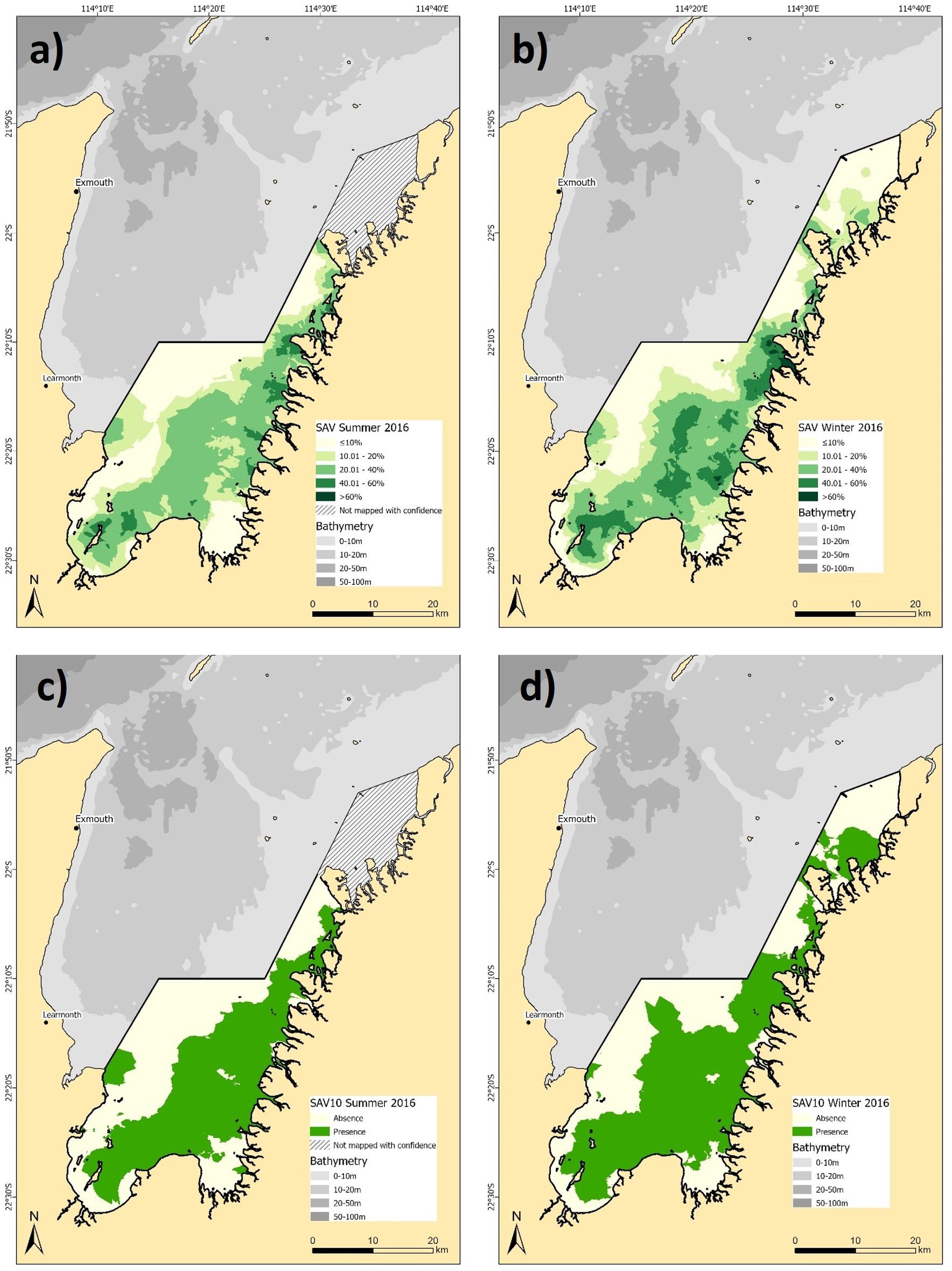
Figure 2. Predicted distribution of submerged aquatic vegetation (SAV) density (a) summer, and (b) winter 2016 and presence/absence for (c) summer, and (d) winter 2016. Note the hashed area in summer 2016 was not mapped with confidence and not included in the seasonal comparison.
3.2.2 Macroalgae
Macroalgae showed seasonal shifts in both density and spatial distribution (Figure 3). Macroalgae distribution across the common extent showed an increase from 446.2 km² in summer (Figure 3a) to 524.5 km² in winter (Figure 3b). Higher density macroalgae areas (>20%) also covered more of the comparable study area in winter compared to summer, with the densest concentrations observed in the southern part of the study area. This indicates substantial seasonal growth of macroalgae during winter. Although, the binary models represented a more conservative estimate of macroalgae distribution in both summer (291.2 km²) and winter (388.8 km²), the overall trends of broader spatial coverage predicted in winter were consistent (Figures 3c, d). The confidence in macroalgae density predictions was moderate to strong, with RMSE values of 16.26% and 9.37% for summer and winter, respectively, while the binary estimates reported overall accuracy of 72.5% and kappa of 0.41 for summer and 75.5% and 0.51 for winter (See Supplementary Table 4 for full confusion matrices).
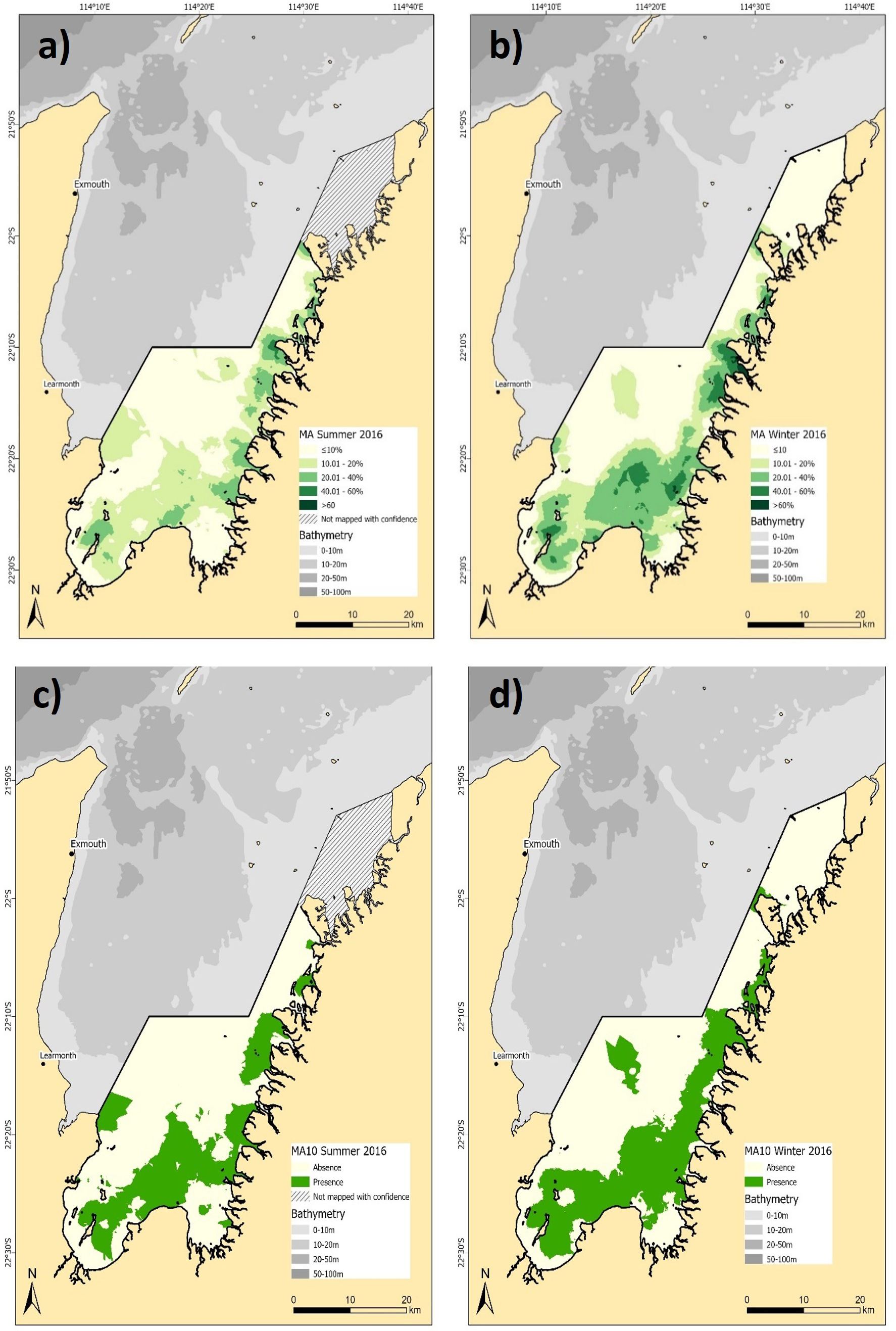
Figure 3. Predicted distribution of macroalgae (MA) density (a) summer, and (b) winter 2016, and, presence/absence for (c) summer, and (d) winter 2016. Note the hashed area in summer 2016 was not mapped with confidence and not included in the seasonal comparison.
3.2.3 Seagrass
Seagrass density and distribution exhibited contrasting dynamics to SAV and macroalgae across the common extent of seasonal habitat mapping, with coverage increasing to 308.4 km² in summer from 209.9 km² in winter (Figures 4a, b). Summer distribution was more widespread, particularly in the southern and eastern areas, while winter coverage remained consistent in the central study area, near Whalebone Island (Figures 4a, b). Density comparisons revealed minimal seasonal changes at the highest density class (20 - 40%) which was similar between seasons (6.74%/66.3 km² in summer; 7.8%/76.3 km² in winter). However, the lower density class (10 - 20%) increased substantially in summer (24.6%/242.1 km²) compared to winter (13.6%/133.7 km²) and was the main driver of the increase in spatial coverage (Figures 4a, b). The more conservative binary models of seagrass distribution estimated a smaller seasonal difference in the total area of seagrass, decreasing only 7.2 km2 between summer (137.1 km2) and winter (129.9 km2) (Figures 4c, d). Seagrass models achieved the highest predictive accuracy of the habitat types, with RMSE values of 16.26% (summer) and 9.37% (winter) for the density models. Binary models showed varying confidence, with the summer model reporting an accuracy of 71.4% and kappa of 0.40, while winter reported 80.2% accuracy and a kappa of 0.46 (See Supplementary Table 4 for full confusion matrices).
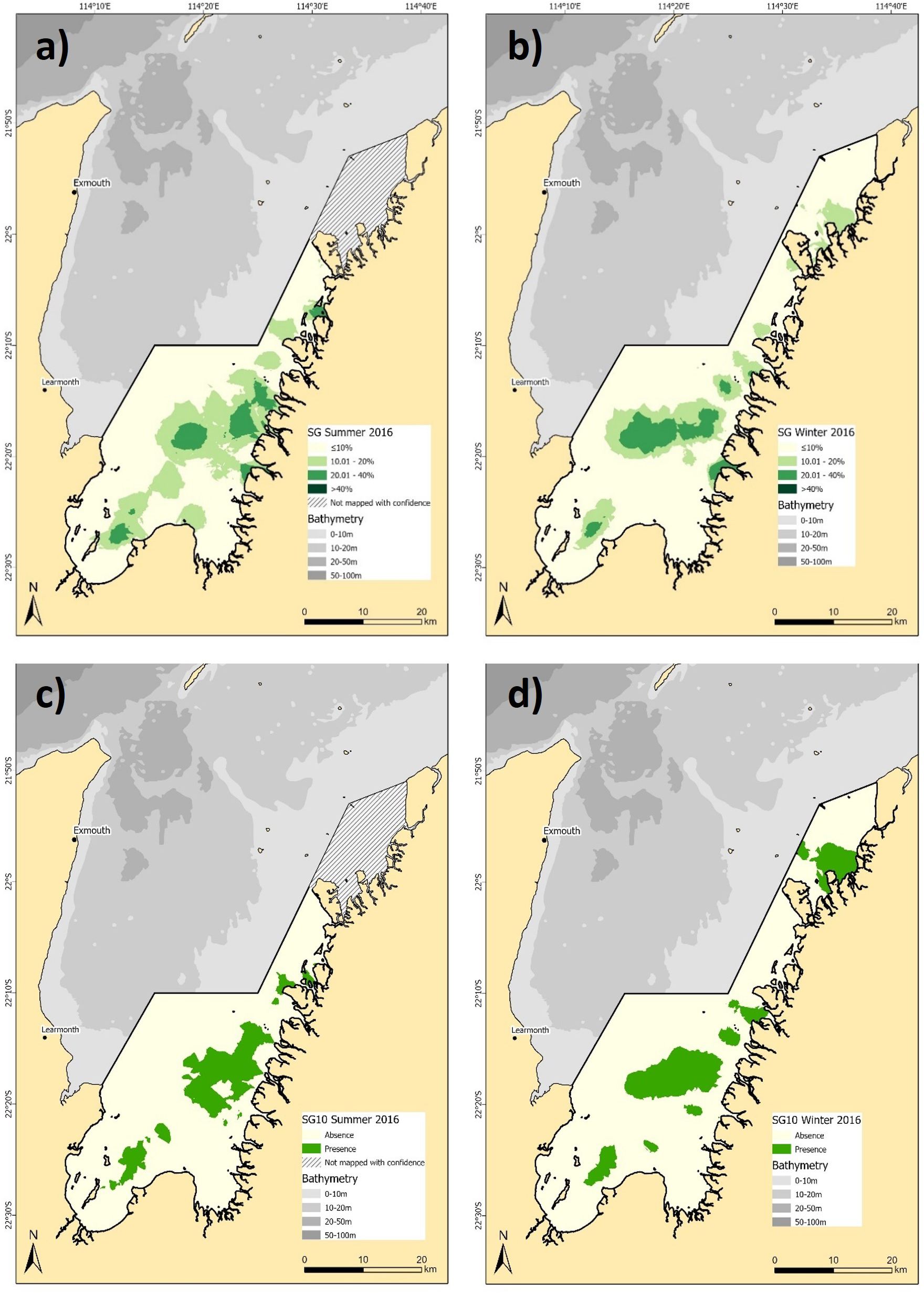
Figure 4. Predicted distribution of seagrass (SG) density (a) summer, and (b) winter 2016, and, presence/absence for (c) summer, and d) winter 2016. Note the hashed area in summer 2016 was not mapped with confidence and not included in seasonal comparisons.
3.2.4 Combined habitat maps for EGPMF nursery grounds
The combined four class binary presence/absence habitat maps (e.g., seagrass, macroalgae, mixed seagrass and macroalgae, and sand) provide a comprehensive view of the spatial and temporal dynamics within the EGPMF nursery grounds (Figure 5). Homogeneous seagrass areas are predominantly found in the central eastern area, covering an estimated area of 92.9 km² (9.5%) in summer (Figure 5a) and 96.4 km² (9.8%) in winter (Figure 5b). Macroalgae also demonstrated high spatial homogeneity, predominantly occupying the southern and eastern nearshore areas of the study area (Figure 5). The extent of macroalgae was estimated to be 247 km² (25.1%) in summer, increasing to 340 km² (34.6%) in winter. Mixed habitats, where seagrass and macroalgae overlap, represent a relatively small proportion of the study area with just 44.2 km² (4.5%) in summer and 52.7 km² (5.4%) in winter (Figures 5a, b). Filter feeders (≥10% abundance) were only observed at six summer ground-truthing sites and five winter sites, with only three reef structure sites (≥10% abundance) observed across both surveys (Figure 5), indicating these habitats are too sparse for robust modelling and are likely sparsely distributed in the study area.
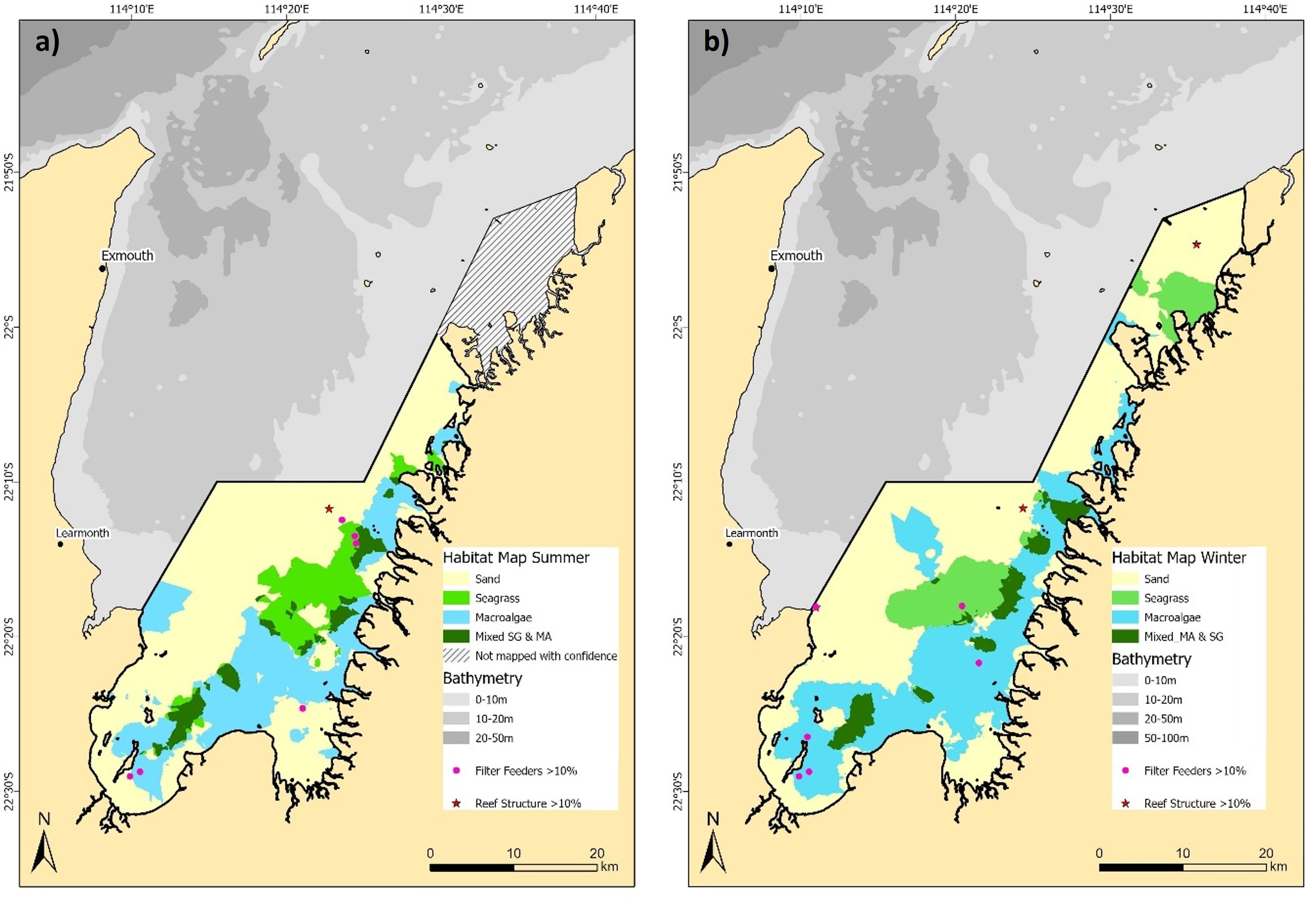
Figure 5. Combined binary (presence/absence) habitat maps for the habitat classes predicted in this study using kriging interpolation for (a) summer, and (b) winter 2016.
Combining the density habitat maps provide more detailed information on the spatial distribution and seasonal dynamics of habitats within the EGPMF nursery grounds (Figure 6), complementing the patterns observed in the binary maps (Figure 5), emphasising that seasonal changes in the study area are primarily driven by shifts in habitat density. In the combined habitat density maps, homogeneous seagrass covers an estimated 131.3 km² of the study area in summer (Figure 6a) and 132.0 km² in winter (Figure 6b). In winter, medium density seagrass accounts for 47 km² (35.6%), with the remaining 85 km² (64.4%) classified as low density, compared to summer, where medium density seagrass covers 28 km² (21.3%) and low density seagrass covers 103 km² (78.7%).
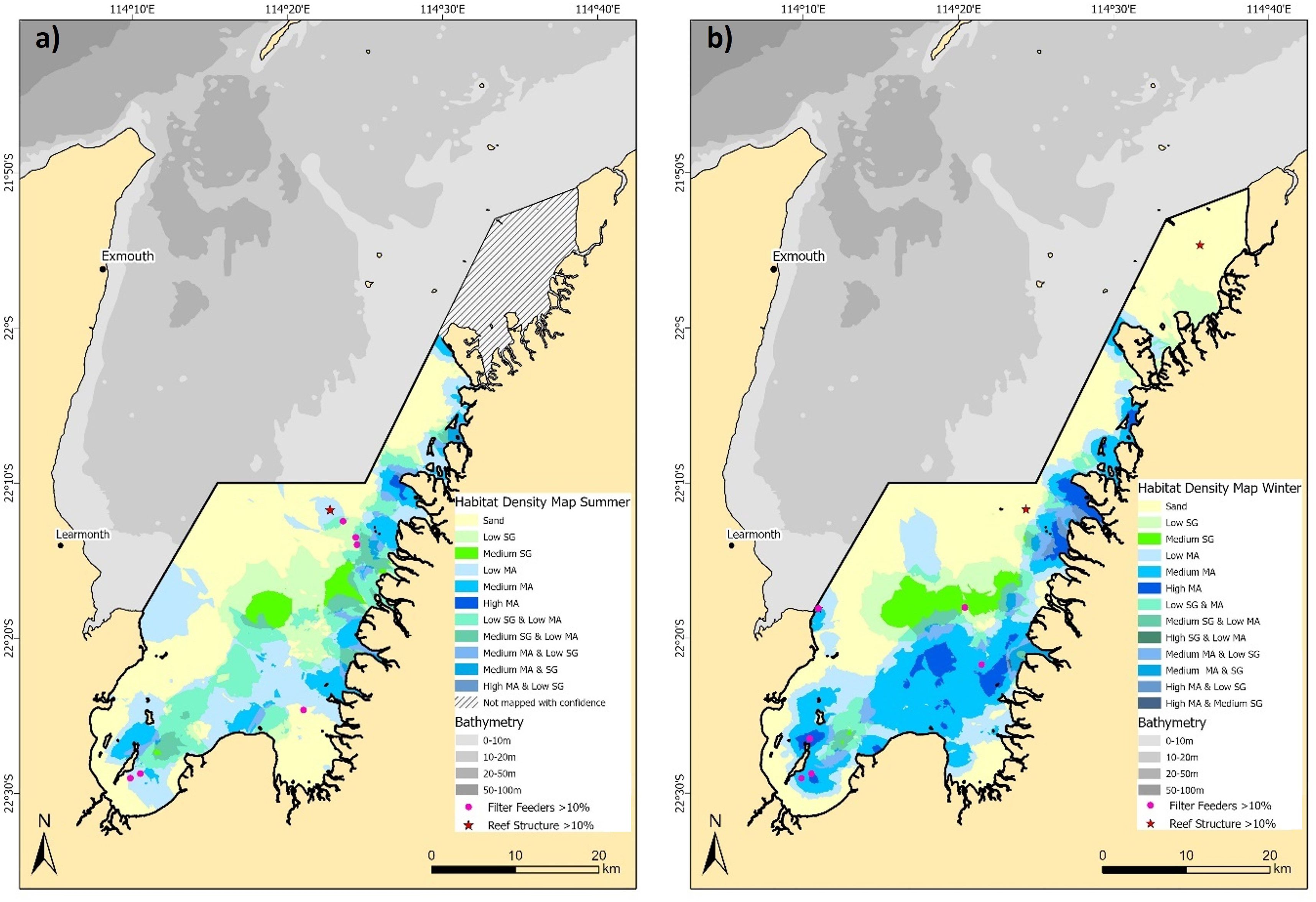
Figure 6. Combined density habitat maps for the habitat classes predicted in this study using kriging interpolation for (a) summer, and (b) winter 2016.
As with the binary estimates of seasonal trends in macroalgae, the density estimates of homogeneous macroalgae shows an increase between summer (276.8 km²) and winter (415.3 km²), particularly in the southeast (Figures 6a, b). The density of homogeneous macroalgae also shifts seasonally, increasing from 0.9% high and 26.5% medium density (remaining 72.6% low density) in summer, to 11.7% high and 51.5% medium density (remaining 36.7% low density) in winter (Figures 6a, b). For overall SAV estimated in the comparable habitat density maps for the summer of 2016 (585 km²), 30.3% (or 177.1 km²) consists of five mixed density assemblage classes, with low-density seagrass/low-density macroalgae (Low SG & Low MA) being the dominant mixed class with 117.3 km² (Figure 6a). Similarly, in winter 2016, the combined SAV estimate of 625 km² includes 16.3% (102.3 km²) of seven mixed density assemblage classes, with low density seagrass/low density macro algae (Low SG & Low MA) again being the dominant mixed class with 37.9 km² (Figure 6b).
This underscores the high degree of homogeneity within the dominant habitat classes and shows increases in both density and distribution of SAV habitats, particularly in the southern and eastern regions of the study area during winter compared to summer.
4 Discussion
4.1 Comparisons of habitat mapping techniques for Exmouth Gulf
Of the four techniques applied, geostatistical kriging was the most robust off-the-shelf method to describe the distribution of benthic habitats in the study area. It demonstrated robust predictive accuracy for both density and presence/absence data, particularly for seagrass and macroalgae. This approach was able to capture spatial patterns with consistent kappa values and high precision, which is essential for supporting evidence-based management (Sharpe et al., 2020; Link and Marshak, 2021; Pennino et al., 2023). Kriging methods are less commonly used for marine habitat mapping due to advancements in remote sensing technology and availability (Malthus and Mumby, 2003; Kutser et al., 2020; Mastrantonis et al., 2024b). Historically, kriging methods have been associated with limitations in predictive accuracy such as sensitivity to uneven data distribution (Legendre and Fortin, 1989). However, given the limitations of satellite remote sensing techniques in turbid environments (McKenzie et al., 2020), our study demonstrated that kriging, combined with spatially balanced data in the modelling process, can result in robust outcomes. By leveraging a spatially comprehensive dataset, kriging was able to effectively capture spatial patterns and reduce uncertainty. This underscores the importance of dataset quality (van der Reijden et al., 2021) and spatial balance in influencing the success of geostatistical models and highlights that with adequate data, kriging remains a valuable tool for marine habitat mapping.
Future developments to enhance the model outputs could incorporate positive outcomes of the other techniques tested, particularly satellite remote sensing and predictive modelling, at a range of scales that may enhance confidence estimates (Diaz et al., 2004; Mastrantonis et al., 2024a; Misiuk and Brown, 2024). Improvements in resolution and the frequency of satellite passes (e.g., 1 to 2 passes per week for Sentinel 2), enables better definition of homogenous habitat categories across large spatial extents in shallow (<5 m) areas by providing a larger repository of imagery to improve the chances of obtaining less turbid, cloud-free imagery (Kuhwald et al., 2022). For example, in our study satellite remote sensing demonstrated strong performance in distinguishing between sand and SAV. The use of ensemble models could further improve certainty of mapped spatial extents (Hossain et al., 2020) However, ensuring compatibility between the model designs and interpretation as well as the quality of training and testing data sets is critical.
Satellite remote sensing offered effective broad scale mapping capabilities for the study area, particularly when ground-truthed using the ≥25% SAV threshold. Both Landsat-8 and Sentinel-2 achieved moderate to high accuracy (75.9% to 81.6%), like other satellite subtidal mapping studies (Rowan and Kalacska, 2021). Yet, underperformed considerably when attempting to further distinguish between habitat like seagrass and macroalgae (kappa <0.12), reflecting challenges in classifying complex habitats from airborne sensors (Wicaksono et al., 2019; Bannari et al., 2022). Off-the-shelf remote sensing tools, while effective for terrestrial landscapes where artefacts such as atmospheric distortion and shadowing are easier to correct, often struggle in aquatic environments due to the dynamic nature of water surfaces, subsurface conditions and depth (Dahdouh-Guebas, 2002; Franklin, 2010). Seasonal variations in turbidity and sensor resolution were shown to influence performance in this study, reducing the reliability of remote sensing for fine scale habitat differentiation compared to the geostatistical modelling approach. These limitations highlight the need for advanced preprocessing techniques and site-specific calibrations to improve classification accuracy in heterogeneous aquatic systems.
Random Forest predictive models also estimated habitat densities of seagrass and SAV well. While they exhibited moderate predictive errors (e.g., RMSE of 10.25% to 23.56% across seasons and habitats), they provided detailed density estimates that complement the geostatistical approach. However, the binary presence/absence models, while achieving high sensitivity, struggled with specificity and false positives. Several factors can contribute to an increase in false positives, including spatial autocorrelation, imbalanced datasets and sampling bias (Legendre and Fortin, 1989; Bradter et al., 2022). The two most likely causes in the current study are the widespread prevalence of suitable conditions, which leads the model to overpredict presence, and the lack of key predictors variables that could improve model specificity. Ephemeral seagrasses that are prevalent in this study area tend to have high spatial and temporal variability, with their distribution often occupying a fraction of suitable habitat available, with processes like dispersal and recruitment influencing distribution within suitable habitat (Hovey et al., 2015). When important environmental or ecological covariates are missing, the model may also struggle to correctly distinguish between suitable and unsuitable habitats, leading to high false positive rates. Incorporating ecologically relevant predictors, such as substrate type, wave energy/hydrodynamics, temperature and benthic light availability, as well as addressing spatial and temporal variability to improve the specificity of predictive models (Fox et al., 2017), will enhance predictive modelling utility for management.
Acoustic sounding at 200 kHz showed promise for mapping broad substrate features, with kappa values reaching 0.80 and high classification accuracy (85% to 93%). This aligns with other studies that showed the 200 kHz distinguishes sediment types and bare substrates from vegetated substrates best (Freitas et al., 2003; Quintino et al., 2010). However, its application for detailed mapping of the sparse benthic biota in the study area was limited by inconsistent alignment with ecological datasets and the high costs associated with surveying such extensive areas. Acoustic mapping generally works better in high density habitats, as dense biological or physical structures (e.g., dense seagrass beds, coral reefs) produce stronger and more consistent acoustic signals that can be more easily differentiated from the surrounding substrate (Gumusay et al., 2019). In contrast, low density habitats often produce weaker or less distinct signals, making it more challenging to interpret the data accurately (Foster et al., 2009). Our findings indicate that while this method effectively detects broad substrate patterns, acoustic sounding alone is insufficient for accurately mapping sparse benthic biota, in part due to the high cost, the need for extensive validation and depth restrictions in this study area.
4.2 Describing and quantifying broad habitats of EGPMF nursery grounds and season changes
While the primary aim of our study was to evaluate ‘off the shelf’ habitat mapping techniques based on confidence matrices to inform EBFM, a valuable by-product was the development of a set of seasonal broad scale habitat maps for the study area. Previous assessments of broadscale habitat abundance and density (McCook et al., 1995; Loneragan et al., 2013; Cartwright et al., 2023), or mapped spatial extents of seagrass (Loneragan et al., 2003), have been both spatial and temporally limited. Our study covered over 50% more area than previously mapped distributions, incorporated seasonal comparisons, and provides estimates of habitat distribution with statistical confidence.
Our study also provided valuable insights into seasonal habitat changes within the EGPMF nursery area. Notably, SAV exhibited greater density and spatial coverage in winter compared to summer. A previous survey of areas within the EGPMF nursery area, which did not make seasonal comparison of macroalgae, found that only 12 of 119 sites surveyed (<10%) had macroalgal cover exceeding 2% in winter (June 1999). However, that study was conducted approximately three months after a category five tropical cyclone which potentially impacted habitat composition (Loneragan et al., 2003). In contrast, our findings, suggest that macroalgae in Exmouth Gulf expand in cooler and more turbid conditions during winter (Cartwright et al., 2021), indicating that macroalgae in Exmouth Gulf may be less affected by turbidity but more sensitive to temperature. However, seagrass was more widely distributed in summer (308.4 km²) than in winter (209.9 km²), with the most notable seasonal shifts occurring at lower densities (10–20%). This contrasts with the previous study which observed a decline in extent from summer to winter (Loneragan et al., 2003). Generally, turbidity within Exmouth Gulf is lower in summer, particularly in the lower Gulf (our study area) (Cartwright et al., 2021). Along with increased sunlight, low turbidity is likely to facilitate seagrass expansion in summer before declining in response to rising turbidity and cooler waters in autumn. As the earlier study was conducted shortly after a cyclone and did not include confidence matrices on the spatial assessments, it is difficult to determine if the observed differences reflect ecological patterns or methodological variation (Loneragan et al., 2003). Disaggregating the environmental drivers of habitat changes (e.g., light, temperature), will further inform fishery and habitat associations for this area.
4.3 Habitat mapping application for management
Our study establishes a valuable baseline for mapping habitat classes relevant to the EGPMF and its nursery area. We also demonstrate the importance of evaluating spatial mapping techniques within the specific context of a study area or fishery resource by incorporating confidence measures to ensure the most reliable spatial outputs are used to inform EBFM (McKee et al., 2021; Davies et al., 2023). For the EGPMF nursery area, while the geostatistical kriging model’s kappa and RMSE values indicate moderate to strong reliability, the observed variance between the presence/absence and percentage density models suggests these spatial maps are best suited for describing broad habitat extents and capturing larger scale shifts. The techniques trialled in this study faced limitations when quantifying the spatial distribution of less common habitats with confidence (e.g., reef and filter feeders) or attempting to disaggregate the broad habitat categories (seagrass and macroalgae) to the genus or species level. Incorporating more rapid analysis of in-situ habitat image data through automated image analysis [e.g (Beijbom et al., 2015; González-Rivero et al., 2020)] may reduce the bottleneck in analysis and allow for the increased collection and evaluation of ground truth habitat data to better inform and validate models. This is critical for improving marine habitat mapping outputs, with improved resolution and associated confidences.
In our study, the ability to disaggregate data across different modelling techniques was also constrained by the limited ecological data available for the study area (Fitzpatrick et al., 2019; Sutton and Shaw, 2021). However, Exmouth Gulf has recently received increased scientific attention, increasing the availability of environmental predictors (Cartwright et al., 2021; Lebrec et al., 2021; Cartwright et al., 2023). With the continued requirement for sustainable management of Exmouth Gulf for a range of users e.g., EGPMF and other commercial, recreational and customary fisheries (Kangas et al., 2015; Banks and McLoughlin, 2017; DPIRD, 2020), conservation sector, and potential industrial development (Sutton and Shaw, 2021), the range of datasets available to inform predictive models will continue to expand. Adopting an iterative approach to integrating these data sources into future habitat mapping could further improve accuracy and enable finer scale and more resolute habitat mapping (Lecours et al., 2015; Bean et al., 2017). This approach would provide a more dynamic and comprehensive framework for habitat assessments, ensuring that management decisions are better informed and more adaptable to changing ecological and socio-economic contexts.
Data availability statement
The raw data supporting the findings of this study are available from the Department of Primary Industries and Regional Development, Western Australia (DPIRD) at www.dpird.wa.gov.au. Access may be granted upon reasonable request, subject to applicable data sharing agreements.
Author contributions
SE: Conceptualization, Data curation, Formal Analysis, Funding acquisition, Investigation, Methodology, Project administration, Resources, Validation, Visualization, Writing – original draft, Writing – review & editing. NK: Conceptualization, Formal Analysis, Investigation, Methodology, Validation, Visualization, Writing – review & editing. RH: Conceptualization, Funding acquisition, Methodology, Supervision, Visualization, Writing – review & editing. GK: Conceptualization, Funding acquisition, Supervision, Writing – review & editing. LB: Conceptualization, Funding acquisition, Project administration, Resources, Supervision, Visualization, Writing – review & editing.
Funding
The author(s) declare that financial support was received for the research and/or publication of this article. This research was supported by the Fisheries Research and Development Corporation (FRDC) on behalf of the Australian Government (Project No. 2015/027). The funder was not involved in the study design, collection, analysis, interpretation of data, the writing of this article or the decision to submit it for publication.
Acknowledgments
The authors acknowledge that this project was supported by funding from the FRDC (2015-027) on behalf of the Australian Government and thank FRDC and DPIRD staff for the administrative support. We are grateful to past and present DPIRD regional service staff for significant logistical support in the Exmouth Gulf Region, as well as past and present DPIRD Aquatic Science and Assessment staff for field and laboratory support. We thank all reviewers, whose input improved the final manuscript.
Conflict of interest
The authors declare that the research was conducted in the absence of any commercial or financial relationships that could be construed as a potential conflict of interest.
Generative AI statement
The author(s) declare that no Generative AI was used in the creation of this manuscript.
Publisher’s note
All claims expressed in this article are solely those of the authors and do not necessarily represent those of their affiliated organizations, or those of the publisher, the editors and the reviewers. Any product that may be evaluated in this article, or claim that may be made by its manufacturer, is not guaranteed or endorsed by the publisher.
Supplementary material
The Supplementary Material for this article can be found online at: https://www.frontiersin.org/articles/10.3389/fmars.2025.1570277/full#supplementary-material
References
Abdo D. A., Bellchambers L. M., and Evans S. N. (2012). Turning up the Heat: Increasing Temperature and Coral Bleaching at the High Latitude Coral Reefs of the Houtman Abrolhos Islands. PloS One 7, e43878. doi: 10.1371/journal.pone.0043878
Althaus F., Hill N., Ferrari R., Edwards L., Przeslawski R., Schönberg C. H. L., et al. (2015). A standardised vocabulary for identifying benthic biota and substrata from underwater imagery: The CATAMI classification scheme. PloS One 10, 1–18. doi: 10.1371/journal.pone.0141039
Arenas-Castro S. and Sillero N. (2021). Cross-scale monitoring of habitat suitability changes using satellite time series and ecological niche models. Sci. Total Environ. 784, 147172. doi: 10.1016/j.scitotenv.2021.147172
Australian Bureau of Meteorology (2022). Climate Data Online. (Melbourne, Australia: Bureau of Meteorology).
Australian Hydrographic Services (2014). Exmouth Gulf and Approaches Nautical Chart (AUS744). (Wollongong, Australia: Australian Hydrographic Office).
Banks R. and McLoughlin K. (2017). Exmouth Gulf Prawn Trawl Fishery, MSC Surveillance Report 1 (MRAG Americas, St Petersburg, Florida, USA: Marine Stewardship Council).
Bannari A., Ali T. S., and Abahussain A. (2022). The capabilities of Sentinel-MSI (2A/2B) and Landsat-OLI (8/9) in seagrass and algae species differentiation using spectral reflectance. Ocean Sci. 18, 361–388. doi: 10.5194/os-18-361-2022
Bastardie F., Brown E. J., Andonegi E., Arthur R., Beukhof E., Depestele J., et al. (2021). A review characterizing 25 ecosystem challenges to be addressed by an ecosystem approach to fisheries management in Europe. Front. Mar. Sci. 7. doi: 10.3389/fmars.2020.629186
Bean T. P., Greenwood N., Beckett R., Biermann L., Bignell J. P., Brant J. L., et al. (2017). A review of the tools used for marine monitoring in the UK: combining historic and contemporary methods with modeling and socioeconomics to fulfill legislative needs and scientific ambitions. Front. Mar. Sci. 4. doi: 10.3389/fmars.2017.00263
Beijbom O., Edmunds P. J., Roelfsema C., Smith J., Kline D. I., Neal B. P., et al. (2015). Towards automated annotation of benthic survey images: variability of human experts and operational modes of automation. PloS One 10, e0130312. doi: 10.1371/journal.pone.0130312
Bradter U., Altringham J. D., Kunin W. E., Thom T. J., O’Connell J., and Benton T. G. (2022). Variable ranking and selection with random forest for unbalanced data. Environ. Data Sci. 1, e30. doi: 10.1017/eds.2022.34
Brown C. J. and Collier J. S. (2008). Mapping benthic habitat in regions of gradational substrata: An automated approach utilising geophysical, geological, and biological relationships. Estuar. Coast Shelf Sci. 78, 203–214. doi: 10.1016/j.ecss.2007.11.026
Brown C. J., Smith S. J., Lawton P., and Anderson J. T. (2011). Benthic habitat mapping: A review of progress towards improved understanding of the spatial ecology of the seafloor using acoustic techniques. Estuar. Coast Shelf Sci. 92, 502–520. doi: 10.1016/j.ecss.2011.02.007
Cartwright P. J., Browne N. K., Belton D., Parnum I., O’Leary M., Valckenaere J., et al. (2023). Long-term spatial variations in turbidity and temperature provide new insights into coral-algal states on extreme/marginal reefs. Coral Reefs 42, 859–872. doi: 10.1007/s00338-023-02393-5
Cartwright P. J., Fearns P. R. C. S., Branson P., Cutler M. V. W., O’leary M., Browne N. K., et al. (2021). Identifying metocean drivers of turbidity using 18 years of modis satellite data: Implications for marine ecosystems under climate change. Remote Sens. (Basel) 13, 3616. doi: 10.3390/rs13183616
Cogan C. B., Todd B. J., Lawton P., and Noji T. T. (2009). The role of marine habitat mapping in ecosystem-based management. ICES J. Marine Sci. 66, 2033–2042. doi: 10.1093/icesjms/fsp214
Conrad O., Bechtel B., Bock M., Dietrich H., Fischer E., Gerlitz L., et al. (2015). System for automated geoscientific analyses (SAGA). Geosci. Model Dev. 8, 1991–2007. doi: 10.5194/gmd-8-1991-2015
Dahdouh-Guebas F. (2002). The use of remote sensing and GIS in the sustainable management of tropical coastal ecosystems. Environ. Dev. Sustain. 4, 93–112. doi: 10.1023/A:1020887204285
Davies S. C., Thompson P. L., Gomez C., Nephin J., Knudby A., Park A. E., et al. (2023). Addressing uncertainty when projecting marine species’ distributions under climate change. Ecography 2023. doi: 10.1111/ecog.06731
Diaz R. J., Solan M., and Valente R. M. (2004). A review of approaches for classifying benthic habitats and evaluating habitat quality. J. Environ. Manage 73, 165–181. doi: 10.1016/j.jenvman.2004.06.004
DPIRD (2020). Ecological Risk Assessment of the Exmouth Gulf Prawn Managed Fishery (Perth, Western Australia: Department of Primary Industries and Regional Development).
DPIRD (2021). Fisheries Management Paper No. 265. Prawn Resource of Exmouth Gulf Harvest Strategy 2021-2026. Version 2.0 (Perth, WA: Department of Primary Industries and Regional Development).
Echoview (2023a). Echoview Habitat Classification Module. Available online at: https://support.echoview.com/WebHelp/_Introduction/Modules/Habitat_Classification.htm?rhhlterm=habitatclassificationmodulemodules&rhsearch=habitatclassificationmodule (Accessed November 15, 2024).
Echoview (2023b). Echoview Bottom Classification Algorithms. Available online at: https://support.echoview.com/WebHelp/Reference/Algorithms/Bottom_Classifcation/Bottom_classification_algorithms.htm (Accessed November 15, 2024).
ESRI (2011). ArcGIS Desktop. (Redlands, California, US: Environmental Systems Research Institute (ESRI)).
ESRI (2023). ArcGIS Pro. (Redlands, California, US: Environmental SystemsResearch Institute (ESRI)).
Evans R. D., McMahon K. M., van Dijk K.-J., Dawkins K., Nilsson Jacobi M., and Vikrant A. (2021). Identification of dispersal barriers for a colonising seagrass using seascape genetic analysis. Sci. Total Environ. 763, 143052. doi: 10.1016/j.scitotenv.2020.143052
Fitzpatrick B., Davenport A., Penrose H., Hart C., Gardner S., Morgan A., et al. (2019). Exmouth Gulf, north Western Australia: A review of environmental and economic values and baseline scientific survey of the south western region (Oceanwise Australia, Exmouth, Western Australia).
Foster G., Walker B. K., and Riegl B. M. (2009). Interpretation of single-beam acoustic backscatter using lidar-derived topographic complexity and benthic habitat classifications in a coral reef environment. J. Coast Res. 10053, 16–26. doi: 10.2112/SI53-003.1
Fox E. W., Hill R. A., Leibowitz S. G., Olsen A. R., Thornbrugh D. J., and Weber M. H. (2017). Assessing the accuracy and stability of variable selection methods for random forest modeling in ecology. Environ. Monit. Assess. 189, 316. doi: 10.1007/s10661-017-6025-0
Franceschini S., Tancioni L., Lorenzoni M., Mattei F., and Scardi M. (2019). An ecologically constrained procedure for sensitivity analysis of Artificial Neural Networks and other empirical models. PloS One 14, e0211445. doi: 10.1371/journal.pone.0211445
Franklin J. (2010). Mapping Species Distributions (Cambridge (UK): Cambridge University Press). doi: 10.1017/CBO9780511810602
Freitas R., Silva S., Quintino V., Rodrigues A. M., Rhynas K., and Collins W. T. (2003). Acoustic seabed classification of marine habitats: studies in the western coastal-shelf area of Portugal. ICES J. Marine Sci. 60, 599–608. doi: 10.1016/S1054-3139(03)00061-4
González-Rivero M., Beijbom O., Rodriguez-Ramirez A., Bryant D. E. P., Ganase A., Gonzalez-Marrero Y., et al. (2020). Monitoring of coral reefs using artificial intelligence: A feasible and cost-effective approach. Remote Sens. (Basel) 12, 489. doi: 10.3390/rs12030489
Gräler B., Pebesma E., and Heuvelink G. (2016). Spatio-Temporal Interpolation using gstat. R J. 8, 204–218. doi: 10.32614/RJ-2016-014
Grizonnet M., Michel J., Poughon V., Inglada J., Savinaud M., and Cresson R. (2017). Orfeo ToolBox: open source processing of remote sensing images. Open Geospatial Data Softw. Standards 2, 15. doi: 10.1186/s40965-017-0031-6
Gumusay M. U., Bakirman T., Tuney Kizilkaya I., and Aykut N. O. (2019). A review of seagrass detection, mapping and monitoring applications using acoustic systems. Eur. J. Remote Sens. 52, 1–29. doi: 10.1080/22797254.2018.1544838
Hickey S. M., Radford B., Roelfsema C. M., Joyce K. E., Wilson S. K., Marrable D., et al. (2020). Between a reef and a hard place: capacity to map the next coral reef catastrophe. Front. Mar. Sci. 7. doi: 10.3389/fmars.2020.544290
Hill N. A., Barrett N., Ford J. H., Peel D., Foster S., Lawrence E., et al. (2018). Developing indicators and a baseline for monitoring demersal fish in data-poor, offshore Marine Parks using probabilistic sampling. Ecol. Indic. 89, 610–621. doi: 10.1016/j.ecolind.2018.02.039
Hossain M. S., Muslim A. M., Nadzri M. I., Teruhisa K., David D., Khalil I., et al. (2020). Can ensemble techniques improve coral reef habitat classification accuracy using multispectral data? Geocarto Int. 35, 1214–1232. doi: 10.1080/10106049.2018.1557263
Hovey R. K., Statton J., Fraser M. W., Ruiz-Montoya L., Zavala-Perez A., Rees M., et al. (2015). Strategy for assessing impacts in ephemeral tropical seagrasses. Mar. Pollut. Bull. 101, 594–599. doi: 10.1016/j.marpolbul.2015.10.054
Jain A. K., Murty M. N., and Flynn P. J. (1999). Data clustering: A review. ACM Comput. Surv. 31, 264–323. doi: 10.1145/331499.331504
Kangas M. I., Sporer E. C., Hesp S. A., Travaille K. L., Moore N., Cavalli P., et al. (2015). Western Australian Marine Stewardship Council Report Series: Exmouth Gulf Prawn Managed Fishery (Perth, Western Australia: Western Australian Department of Fisheries).
Krige D. G. (1951). A statistical approach to some basic mine valuation problems on the Witwatersrand. J. South Afr. Inst. Min. Metall. 52, 119–139. doi: 10.10520/AJA0038223X_4792
Kruss A., Wiktor J., Wiktor J., and Tatarek A. (2019). “Acoustic detection of macroalgae in a dynamic Arctic environment (Isfjorden, West Spitsbergen) using multibeam echosounder,” in 2019 IEEE International Underwater Technology Symposium, UT 2019 - Proceedings (Piscataway (NJ), USA: IEEE). doi: 10.1109/UT.2019.8734323
Kuhn M. (2008). Building predictive models in R using the caret package. J. Stat. Softw. 28, 1–26. doi: 10.18637/jss.v028.i05
Kuhwald K., Schneider von Deimling J., Schubert P., and Oppelt N. (2022). How can Sentinel-2 contribute to seagrass mapping in shallow, turbid Baltic Sea waters? Remote Sens. Ecol. Conserv. 8, 328–346. doi: 10.1002/rse2.246
Kutser T., Hedley J., Giardino C., Roelfsema C., and Brando V. E. (2020). Remote sensing of shallow waters – A 50 year retrospective and future directions. Remote Sens. Environ. 240, 111619. doi: 10.1016/j.rse.2019.111619
Lebrec U., Paumard V., O’Leary M. J., and Lang S. C. (2021). Towards a regional high-resolution bathymetry of the North West Shelf of Australia based on Sentinel-2 satellite images, 3D seismic surveys, and historical datasets. Earth Syst. Sci. Data 13, 5191–5212. doi: 10.5194/essd-13-5191-2021
Lecours V. (2017). On the use of maps and models in conservation and resource management (Warning: results may vary). Front. Mar. Sci. 4. doi: 10.3389/fmars.2017.00288
Lecours V., Devillers R., Schneider D., Lucieer V., Brown C., and Edinger E. (2015). Spatial scale and geographic context in benthic habitat mapping: review and future directions. Mar. Ecol. Prog. Ser. 535, 259–284. doi: 10.3354/meps11378
Legendre P. and Fortin M. J. (1989). Spatial pattern and ecological analysis. Vegetatio 80, 107–138. doi: 10.1007/BF00048036
Li J. and Heap A. D. (2014). Spatial interpolation methods applied in the environmental sciences: A review. Environ. Model. Softw. 53, 173–189. doi: 10.1016/j.envsoft.2013.12.008
Liaw A. and Wiener M. (2002). The R Journal: Classification and regression by randomForest. R J. 2, 18–22.
Link J. S. and Marshak A. R. (2021). Ecosystem-Based Fisheries Management (Oxford: Oxford University Press). doi: 10.1093/oso/9780192843463.001.0001
Loneragan N. R., Kangas M., Haywood M. D. E., Kenyon R. A., Caputi N., and Sporer E. (2013). Impact of cyclones and aquatic macrophytes on recruitment and landings of tiger prawns penaeus esculentus in exmouth gulf, western Australia. Estuar. Coast Shelf Sci. 127, 46–58. doi: 10.1016/j.ecss.2013.03.024
Loneragan N. R., Kenyon R. A., Crocos P. J., Ward R. D., Lehnert S., Haywood M. D. E., et al. (2003). Developing techniques for enhancing prawn fisheries, with a focus on brown tiger prawns (Penaeus esculentus) in Exmouth Gulf. Final Report on FRDC Project 1999/222 (Cleveland: CSIRO Marine Research).
Lovelock C. E., Feller I. C., Adame M. F., Reef R., Penrose H. M., Wei L., et al. (2011). Intense storms and the delivery of materials that relieve nutrient limitations in mangroves of an arid zone estuary. Funct. Plant Biol. 38, 514. doi: 10.1071/FP11027
Lu D. and Weng Q. (2007). A survey of image classification methods and techniques for improving classification performance. Int. J. Remote Sens. 28, 823–870. doi: 10.1080/01431160600746456
Madin J. S. and Madin E. M. P. (2015). The full extent of the global coral reef crisis. Conserv. Biol. 29, 1724–1726. doi: 10.1111/cobi.12564
Main-Knorn M., Pflug B., Louis J., Debaecker V., Müller-Wilm U., and Gascon F. (2017). “Sen2Cor for sentinel-2,” in Image and Signal Processing for Remote Sensing XXIII. Eds. Bruzzone L., Bovolo F., and Benediktsson J. A. (Bellingham (WA): SPIE), 3. doi: 10.1117/12.2278218
Malthus T. J. and Mumby P. J. (2003). Remote sensing of the coastal zone: An overview and priorities for future research. Int. J. Remote Sens. 24, 2805–2815. doi: 10.1080/0143116031000066954
Mastrantonis S., Langlois T., Radford B., Spencer C., de Lestang S., and Hickey S. (2024a). Revealing the impact of spatial bias in survey design for habitat mapping: A tale of two sampling designs. Remote Sens. Appl. 36, 101327. doi: 10.1016/j.rsase.2024.101327
Mastrantonis S., Radford B., Langlois T., Spencer C., de Lestang S., and Hickey S. (2024b). A novel method for robust marine habitat mapping using a kernelised aquatic vegetation index. ISPRS J. Photogramm. Remote Sens. 209, 472–480. doi: 10.1016/j.isprsjprs.2024.02.015
McCook L., Klumpp D., and McKinnon A. (1995). Seagrass communities in Exmouth Gulf, Western Australia: A preliminary survey. J. R Soc. West Aust. 78, 81–87.
McKee A., Grant J., and Barrell J. (2021). Mapping American lobster (Homarus americanus) habitat for use in marine spatial planning. Can. J. Fisheries Aquat. Sci. 78, 704–720. doi: 10.1139/cjfas-2020-0051
McKenzie L. J., Langlois L. A., and Roelfsema C. M. (2022). Improving approaches to mapping seagrass within the great barrier reef: from field to spaceborne earth observation. Remote Sens. (Basel) 14, 2604. doi: 10.3390/rs14112604
McKenzie L. J., Nordlund L. M., Jones B. L., Cullen-Unsworth L. C., Roelfsema C., and Unsworth R. K. F. (2020). The global distribution of seagrass meadows. Environ. Res. Lett. 15, 074041. doi: 10.1088/1748-9326/ab7d06
McMahon K., Hernawan U., van Dijk K., Waycott M., Biffin E., Evans R., et al. (2017). Genetic variability within seagrass of the north west of Western Australia. Report of Theme 5 - Project 5.2 prepared for the Dredging Science Node, Western Australian Marine Science Institution (Perth, Western Australia).
Melo-Merino S. M., Reyes-Bonilla H., and Lira-Noriega A. (2020). Ecological niche models and species distribution models in marine environments: A literature review and spatial analysis of evidence. Ecol. Modell. 415, 108837. doi: 10.1016/j.ecolmodel.2019.108837
Menandro P. S., Lavagnino A. C., Vieira F. V., Boni G. C., Franco T., and Bastos A. C. (2022). The role of benthic habitat mapping for science and managers: A multi-design approach in the Southeast Brazilian Shelf after a major man-induced disaster. Front. Mar. Sci. 9. doi: 10.3389/fmars.2022.1004083
Misiuk B. and Brown C. J. (2024). Benthic habitat mapping: A review of three decades of mapping biological patterns on the seafloor. Estuar. Coast Shelf Sci. 296, 108599. doi: 10.1016/j.ecss.2023.108599
Moore C., Drazen J. C., Radford B. T., Kelley C., and Newman S. J. (2016). Improving essential fish habitat designation to support sustainable ecosystem-based fisheries management. Mar. Policy 69, 32–41. doi: 10.1016/j.marpol.2016.03.021
Mumby P. J., Chisholm J. R. M., Clark C. D., Hedley J. D., and Jaubert J. (2001). A bird’s-eye view of the health of coral reefs. Nature 413, 36–36. doi: 10.1038/35092617
Norberg A., Abrego N., Blanchet F. G., Adler F. R., Anderson B. J., Anttila J., et al. (2019). A comprehensive evaluation of predictive performance of 33 species distribution models at species and community levels. Ecol. Monogr. 89, e01370. doi: 10.1002/ecm.1370
Orth R. J., Carruthers T. J. B., Dennison W. C., Duarte C. M., Fourqurean J. W., Heck K. L., et al. (2006). A global crisis for seagrass ecosystems. Bioscience 56, 987–996. doi: 10.1641/0006-3568(2006)56[987:AGCFSE]2.0.CO;2
Overly K. E. and Lecours V. (2024). Mapping queen snapper (Etelis oculatus) suitable habitat in Puerto Rico using ensemble species distribution modeling. PloS One 19, e0298755. doi: 10.1371/journal.pone.0298755
Pebesma E. (2004). Multivariable geostatistics in S: the gstat package. Comput. Geosci. 30, 683–691. doi: 10.1016/j.cageo.2004.03.012
Pennino M. G., Rehren J., Tifoura A., Lojo D., and Coll M. (2023). New approaches to old problems: how to introduce ecosystem information into modern fisheries management advice. Hydrobiologia 850, 1251–1260. doi: 10.1007/s10750-022-05083-5
Phillips S. J., Anderson R. P., and Schapire R. E. (2006). Maximum entropy modeling of species geographic distributions. Ecol. Modell. 190, 231–259. doi: 10.1016/j.ecolmodel.2005.03.026
Pickens B. A., Carroll R., Schirripa M. J., Forrestal F., Friedland K. D., and Taylor J. C. (2021). A systematic review of spatial habitat associations and modeling of marine fish distribution: A guide to predictors, methods, and knowledge gaps. PloS One 16, e0251818. doi: 10.1371/journal.pone.0251818
Quintino V., Freitas R., Mamede R., Ricardo F., Rodrigues A. M., Mota J., et al. (2010). Remote sensing of underwater vegetation using single-beam acoustics. ICES J. Marine Sci. 67, 594–605. doi: 10.1093/icesjms/fsp251
R Core Team (2023). R: A language for Statistical Computing (Vienna, Austria: R Foundation for Statistical Computing).
Robinson N. M., Nelson W. A., Costello M. J., Sutherland J. E., and Lundquist C. J. (2017). A systematic review of marine-based species distribution models (SDMs) with recommendations for best practice. Front. Mar. Sci. 4. doi: 10.3389/fmars.2017.00421
Roelfsema C. M., Kovacs E. M., Ortiz J. C., Callaghan D. P., Hock K., Mongin M., et al. (2020). Habitat maps to enhance monitoring and management of the Great Barrier Reef. Coral Reefs 39, 1039–1054. doi: 10.1007/s00338-020-01929-3
Rowan G. S. L. and Kalacska M. (2021). A review of remote sensing of submerged aquatic vegetation for non-specialists. Remote Sens. (Basel) 13, 623. doi: 10.3390/rs13040623
Rubbens P., Brodie S., Cordier T., Destro Barcellos D., Devos P., Fernandes-Salvador J. A., et al. (2023). Machine learning in marine ecology: an overview of techniques and applications. ICES J. Marine Sci. 80, 1829–1853. doi: 10.1093/icesjms/fsad100
Schultz S. T., Kruschel C., Bakran-Petricioli T., and Petricioli D. (2015). Error, power, and blind sentinels: the statistics of seagrass monitoring. PloS One 10, e0138378. doi: 10.1371/journal.pone.0138378
Semeniuk V. (1985). Development of mangrove habitats along ria shorelines in north and northwestern tropical Australia. Vegetatio 60, 3–23. doi: 10.1007/BF00053907
Sharpe L. M., Hernandez C. L., and Jackson C. A. (2020). Prioritizing Stakeholders, Beneficiaries, and Environmental Attributes: A Tool for Ecosystem-Based Management. Ecosystem-Based Management, Ecosystem Services and Aquatic Biodiversity (Cham: Springer International Publishing), 189–211. doi: 10.1007/978-3-030-45843-0_10
Shumchenia E. J. and King J. W. (2010). Comparison of methods for integrating biological and physical data for marine habitat mapping and classification. Cont. Shelf Res. 30, 1717–1729. doi: 10.1016/j.csr.2010.07.007
Smith Menandro P. and Cardoso Bastos A. (2020). Seabed mapping: A brief history from meaningful words. Geosci. (Basel) 10, 273. doi: 10.3390/geosciences10070273
Strydom S., Murray K., Wilson S., Huntley B., Rule M., Heithaus M., et al. (2020). Too hot to handle: Unprecedented seagrass death driven by marine heatwave in a World Heritage Area. Glob. Chang. Biol. 26, 3525–3538. doi: 10.1111/gcb.15065
Sutton A. L. and Shaw J. L. (2021). Cumulative Pressures on the Distinctive Values of Exmouth Gulf. First draft report to the Department of Water and Environmental Regulation by the Western Australian Marine Science Institution (Perth, Western Australia: Western Australian Marine Science Institution).
Thuiller W., Georges D., Gueguen M., Engler R., Breiner F., Lafourcade B., et al. (2023). Package “biomod2” Title Ensemble Platform for Species Distribution Modeling (Vienna Austria: Comprehensive R Archive Network (CRAN)), Vol. 135.
Tomczak M. and Godfrey J. S. (2003). Regional oceanography: an introduction (Daya Publishing House; Delhi, India: Daya books).
Townsend H., Harvey C. J., deReynier Y., Davis D., Zador S. G., Gaichas S., et al. (2019). Progress on implementing ecosystem-based fisheries management in the United States through the use of ecosystem models and analysis. Front. Mar. Sci. 6. doi: 10.3389/fmars.2019.00641
Vanderklift M., Bearham D., Haywood M., Lozano-Montes H., McCallum R., McLaughlin J., et al. (2016). Natural dynamics: understanding natural dynamics of seagrasses of the north west of Western Australia. Report of Theme 5 - Project 5.3 prepared for the Dredging Science Node (Perth, Western Australia: Western Australian Marine Science Institution).
van der Reijden K. J., Govers L. L., Koop L., Damveld J. H., Herman P. M. J., Mestdagh S., et al. (2021). Beyond connecting the dots: A multi-scale, multi-resolution approach to marine habitat mapping. Ecol. Indic. 128, 107849. doi: 10.1016/j.ecolind.2021.107849
Ware S. and Downie A.-L. (2020). Challenges of habitat mapping to inform marine protected area (MPA) designation and monitoring: An operational perspective. Mar. Policy 111, 103717. doi: 10.1016/j.marpol.2019.103717
Wicaksono P., Fauzan M. A., Kumara I. S. W., Yogyantoro R. N., Lazuardi W., and Zhafarina Z. (2019). Analysis of reflectance spectra of tropical seagrass species and their value for mapping using multispectral satellite images. Int. J. Remote Sens. 40, 8955–8978. doi: 10.1080/01431161.2019.1624866
Wu Y.-H. and Hung M.-C. (2016). Comparison of Spatial Interpolation Techniques Using Visualization and Quantitative Assessment (London (UK): Applications of Spatial Statistics, InTech). doi: 10.5772/65996
Wulder M. A., Roy D. P., Radeloff V. C., Loveland T. R., Anderson M. C., Johnson D. M., et al. (2022). Fifty years of Landsat science and impacts. Remote Sens. Environ. 280, 113195. doi: 10.1016/j.rse.2022.113195
Keywords: marine habitat mapping, confidence statistics, Exmouth Gulf, remote sensing, machine learning, EBFM
Citation: Evans SN, Konzewitsch N, Hovey RK, Kendrick GA and Bellchambers LM (2025) Selecting the best habitat mapping technique: a comparative assessment for fisheries management in Exmouth Gulf. Front. Mar. Sci. 12:1570277. doi: 10.3389/fmars.2025.1570277
Received: 03 February 2025; Accepted: 24 April 2025;
Published: 22 May 2025.
Edited by:
Francois Bastardie, Technical University of Denmark, DenmarkReviewed by:
Jessica Garcia, University of Corsica Pascal Paoli, FranceRobert Mzungu Runya, Marine Institute, Ireland
Copyright © 2025 Evans, Konzewitsch, Hovey, Kendrick and Bellchambers. This is an open-access article distributed under the terms of the Creative Commons Attribution License (CC BY). The use, distribution or reproduction in other forums is permitted, provided the original author(s) and the copyright owner(s) are credited and that the original publication in this journal is cited, in accordance with accepted academic practice. No use, distribution or reproduction is permitted which does not comply with these terms.
*Correspondence: Scott N. Evans, c2NvdHQuZXZhbnNAZHBpcmQud2EuZ292LmF1