Automated denoising techniques for sea surface temperature and salinity data from opportunity vessels: application to the Ocean Globe Race 2023-2024

Ever more often, opportunity vessels are used to provide in-situ sea surface temperature and salinity data. In particular, sailing vessels participating in oceanic races are often utilized, as they usually cover remote areas not reached by commercial vessels, such as the southern oceans. The received signal from temperature and salinity sensors -especially the latter- is often disturbed either by bubbles, due to strong turbulent flows, or by non-renewal of the water in contact with the sensor. Until now, only manual methods have been successfully used to filter this data, since no automated procedure has been developed. In this paper, we present (i) a sensor housing to be placed on the keel, designed to reduce the aforementioned physical issues, and (ii) an automatic filtering method to override the manual procedure. The physical system was mounted on the historic sailboat Pen Duick VI and has served to collect data along the Ocean Globe Race route (2023-2024). This initiative was a collaboration between the crew of the boat, the Institute of Marine Sciences (ICM-CSIC) in Barcelona, and the Laboratoire d’Océanographie Physique et Spatiale (Ifremer). The housing for sensors consisted of a 3D-printed hydrodynamic support, designed to reduce drag. The automated filtering approach was based on wavelet denoising techniques and simple moving averages. The results are presented in an open dataset and show that procedure yielded good performance in identifying and rejecting outliers, while operating with far greater speed than manual filtering. The method is intended to become a standard procedure for similar in-situ datasets, and an open-source software is provided for this purpose. This work is a step forward in oceanographic data processing and aims to provide a tool with a wide range of applications.

1 Introduction

On 8 September 1973, 17 yachts and 167 crew members departed from Portsmouth, United Kingdom, to complete what was about to become the first-ever round-the-world sailing race: the Whitbread Round the World Race. Since that historic edition, the race has been held every three or four years, evolving under different names, including the Volvo Ocean Race (2001-2018) and currently, The Ocean Race. These regattas have always pushed the limits of human and technological endurance, serving as a testing ground for innovation in boat design, engineering, and navigation.

While technological advancements have led to the development of increasingly sophisticated and efficient sailing vessels, some boats from the early editions remain highly capable of undertaking global voyages. Recognizing their enduring value was conceived the Ocean Globe Race (OGR), to allow these classic yachts to sail around the world once again. Its first edition commenced in September 2023, and a second edition is planned for 2027.

From an oceanographic perspective, these long-distance sailing races represent unique opportunities for collecting in-situ data in some of the most remote and least-sampled areas of the world’s oceans, particularly the Southern Ocean Chapman et al. (2020). The high-latitude regions covered by these regattas are crucial for understanding ocean-climate interactions, yet they remain severely undersampled due to access difficulties and harsh conditions. In-situ measurements collected by vessels participating in these long-distance sailing races contribute to valuable datasets for validating satellite observations, improving climate models, and enhancing our understanding of ocean dynamics in these extreme and remote environments Behncke et al. (2024); Landschützer et al. (2023); Tanhua et al. (2020).

The use of racing yachts as vessels of opportunity in oceanography involves significant challenges regarding data quality control and processing. Measurements of sea surface temperature (SST) and sea surface salinity (SSS) collected from these platforms are frequently affected by instrumental noise arising from two primary issues: (i) the formation of air bubbles due to high-speed turbulent flows around the sensor, and (ii) the lack of continuous renewal of water in contact with the sensor, leading to stagnation induced errors. Until now, manual filtering techniques have been the primary method for correcting such disturbances, limiting the scalability and efficiency of data processing. During the 2010s, efforts have been made to use automatic denoising techniques (Gourrion et al. (2020) and references therein).

Building on previous oceanographic initiatives in global sailing races, the present study integrates lessons learned from over a decade of experience in equipping regatta vessels with oceanographic sensors. The first successful deployment of scientific instrumentation on a competitive sailing yacht occurred in 2011 through a collaboration between the Barcelona World Race (BWR-2011) organizers, the Institute of Marine Sciences (ICM-CSIC), and the Maritime Catalan Forum (FMC). A MicroCAT (SBE-37) temperature and conductivity sensor, alongside an XCAT transmitter, enabled real-time transmission of sea surface data, demonstrating that scientific measurements could be collected without interfering with navigation or race performance Salat et al. (2013). This success led to continued sensor deployments in subsequent races, including the Barcelona World Race 2014-2015 (BWR-2015) and the Vendée Globe Race 2020-2021 (VGR-2020/2021) Umbert et al. (2022). All these experiences provided valuable high-resolution in-situ SST and SSS datasets along remote oceanic routes and served to validate satellite products in the Southern Ocean. Recent work by Hernani et al. (2025) highlighted the ability of regatta sailboats to collect high-resolution SST and SSS data across the Southern Ocean during the last decade, identifying significant interannual variability and linking observed changes to major climate drivers such as the El Nino–Southern˜ Oscillation (ENSO) and the Southern Annular Mode (SAM).

The present study describes two key innovations to address the above mentioned challenges: (i) the development of a sensor housing system to be mounted on the keel of the vessel, designed to minimize bubble formation and water stagnation effects, and (ii) the implementation of a fully automated filtering method to replace manual data processing. The newly designed hydrodynamic sensor housing was deployed on the historic sailing vessel Pen Duick VI during the Ocean Globe Race 2023-2024, in collaboration with the Institute of Marine Sciences (ICM-CSIC) in Barcelona and the French Institute for Research and Exploitation of the Sea (IFREMER).

2 Data

2.1 Course of the 2023 Ocean Globe Race

SST and SSS data were collected along the race course followed by Pen Duick VI in the 2023 Ocean Globe Race, starting in Southampton (UK) on September 10, 2023, and ending on April 16, 2024, at the same harbor. The race consisted of four legs around the globe, from which only legs 2, 3, and 4 have been considered in the present data collection, as no water samples were collected in the first leg to check for possible salinity drifts (see Figure 1). On these three legs, the sensor took one measure per minute, resulting in 215,343 pairs of raw temperature and salinity (see Table 1).

Figure 1

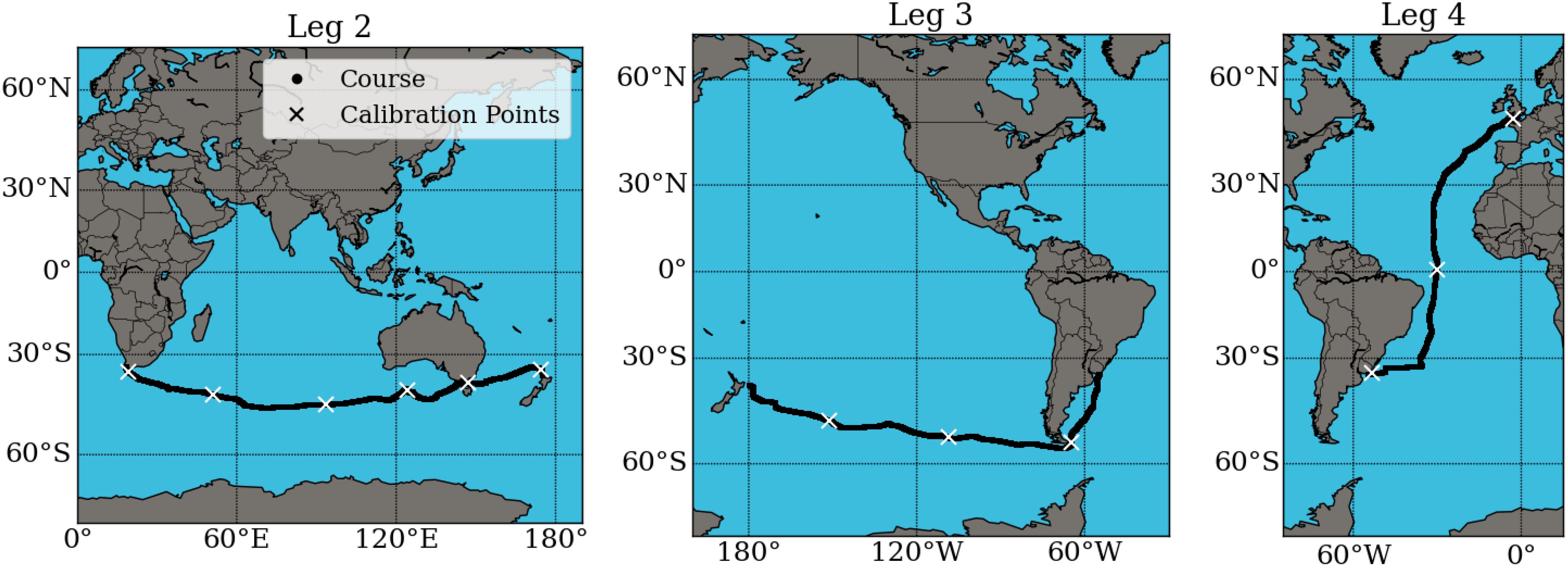
Figure 1. Ship course during Legs 2, 3, and 4 of the race, with water sampling points marked along the route.

Table 1

Table 1. Summary of the Ocean Globe Race 2023–2024 legs with corresponding dates, harbors, and number of salinity/temperature measurements collected.

2.2 Sensor

Data collection was conducted using an NKE STPS300 data logger, which measures temperature, conductivity, and pressure. This instrument has a range of optimal performance for depths up to 300 m and is powered by an internal battery. It operates within a temperature range of -5 to 35 °C with an accuracy of 0.05 °C. The conductivity sensor has a measurement range of 0 to 70 mS/cm and an accuracy of 0.05 mS/cm, which gives an accuracy of 0.10 in practical salinity. Calibration of the sensor is conducted following each battery replacement, to maintain measurement accuracy. The most recent battery replacement and associated calibration were performed in January 2021. Water samples were collected during the race course to allow posterior salinity data correction. The sensor was installed on the keel of Pen Duick VI in September 2023. Geospatial data were provided by the onboard external GPS. Data collection was performed at a sampling frequency of one sample per minute.

2.3 Samples for salinity corrections

To assess possible biases in salinity data, along the course of Legs 2, 3, and 4, seawater samples were collected at specific control points. Their locations were meant to be regularly distributed over distance. However the exact locations mainly depended on the possibilities of the crew in a racing context. Furthermore, the number of sampling points was limited by the storage space available on board.

At each control point, three 250 ml plastic flasks of seawater were collected and stored for post-cruise salinity analysis at the Laboratoire d’Océanographie Physique et Spatiale - UMR 6523 IFREMER, using a Portasal LOPS-E salinometer. Given that plastic containers are not standard in high-precision oceanographic sampling protocols, several precautions were taken to preserve sample quality: each flask was thoroughly rinsed with sample water prior to collection and then filled carefully to minimize headspace. The bottles were sealed with their original caps and additionally secured using Teflon tape and electrical tape to enhance hermetic sealing. Samples were stored in the coolest, darkest available location on board to minimize temperature fluctuations and evaporation. This being said, given our target accuracy of 0.1 in practical salinity in the context of this global-scale study, any potential impact from contamination or evaporation is considered negligible. In Table 2, the average value from every triple measure (S_ref) and the corresponding standard deviation (STD) are shown. These triple measure values are taken as S reference for the control points.

Table 2

Table 2. Salinity measurements from water samples taken during the PenDuick VI cruise.

2.4 Sensor housing

Previous studies involving in-situ measurements of temperature and salinity commonly installed the sensors inside the hull of the ship, in the box housing the articulation of the swing keel. Although this box was open and below the waterline, ensuring good renewal of the water, it was exposed to bubbles in rough weather and may remain even dry in heeling or upwind sailing situations Umbert et al. (2022). Since the renewal of water in contact with the sensor is a critical factor, in the present work, the sensor is placed on top of the keel bulb, therefore outside the hull and in direct contact with the seawater (Figure 2). This configuration avoids issues related to the water intake system and ensures continuous water renewal.

Figure 2

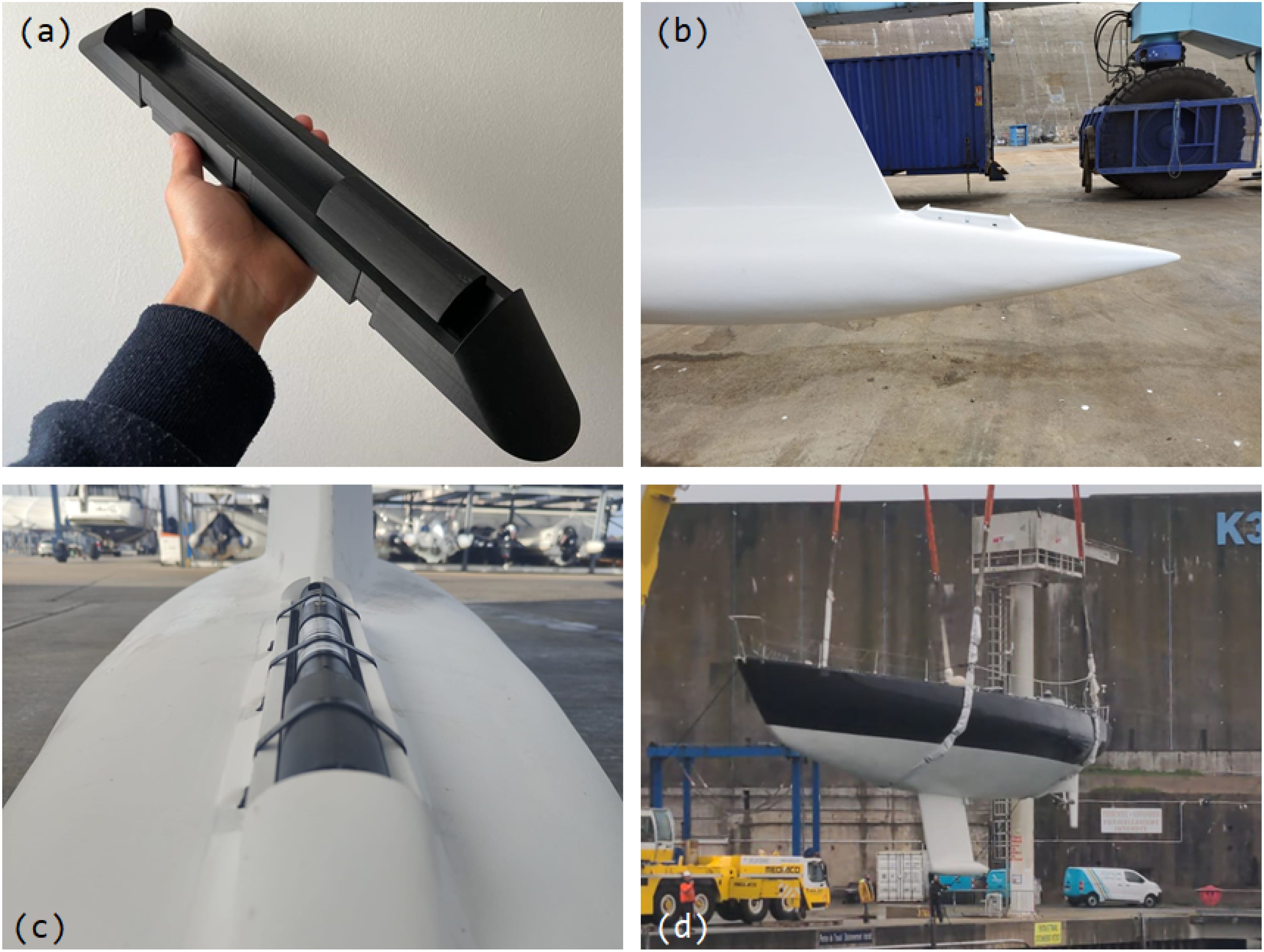
Figure 2. (a) 3D printed sensor housing. (b, c) Sensor housing location in the keel of the sailboat. (d) Pen Duick VI hull shape.

For this purpose, the new sensor housing design must avoid as much as possible having any mechanical impact on the hull of the sailing vessel. Given that the boat will be used for racing purposes, the objective is to interfere as little as possible with its performance and to minimize the increase of its hydrodynamic resistance. At the same time, the housing must protect the sensor to ensure that it remains undamaged in the event of a collision with an object, while also ensuring that the flow reaching the sensing cell remains unobstructed. The sensor has been installed directly on top of the keel bulb using a custom-designed support structure developed to accommodate the specific sensor in use. The housing was manufactured using 3D printing, a particularly advantageous fabrication method for applications requiring unique and custom-made components. This approach significantly reduces costs compared to the use of other materials or modifications to existing products. Moreover, 3D printing minimizes waste, as the material is directly formed into the final product, ensuring an efficient and sustainable manufacturing process.

The 3D model of the designed housing includes designated areas for bolting it to the vessel hull, as well as recesses to accommodate ties that secure the sensor. The design enables easy removal and re-installation of the sensor for cleaning or maintenance without detaching the housing from the hull. The dimensions of the support structure are 450 x 90 x 50 mm. The ends of the housing have been contoured to minimize hydrodynamic resistance (Figure 2). The location is behind the keel fin to reduce the impact probability with floating objects. In this position, the sensor is submerged at a depth ranging from 2.5 to 3.5 meters, which helps reduce the presence of foam and ensures more accurate measurements.

3 Methodology

3.1 Data filtering

Raw data from opportunity vessels is commonly noisy and needs filtering. For this kind of data, the process has historically been done through plotting the time series and manually suppressing outliers. In this section, an automation of this process is presented, for which software has been developed.

3.1.1 General procedure

The method uses the following standard quality control (QC) flags: 0 for no QC performed, 1 for good data, 2 for probably good data, 3 for probably bad data, 4 for bad data, and 6 for harbor data¹.

First, the data is parsed so that only points labeled with QC< 3 are considered. Then two kinds of denoising processes are followed: wavelet denoising (WD) and moving average denoising (AD), the two of them detailed in the following subsections. Both WD and AD take as input a time series and produce a new one, which has the same number of points and is a less noisy representation of the input.

After each denoising process (WD or AD), a quality control is applied to the original data following this principle: the more the original data points differ from the corresponding value in the denoised time series, the “worse” it is their assigned QC flag. When various rounds of (denoising + QC) are applied, each round only works with data labeled with QC< 3, as a result of all previous rounds. It is also respected that none of the quality controls can be “improved” by any of these steps, that is, QC at step n must be greater than or equal to the QC at step n − 1. In this way, at every round, denoising happens on a subset of the data considered in the previous step.

Let δ_ibe the distance between the i-th value in the original data and the corresponding value in the denoised representation. For comparing the two time series and setting QC labels, three thresholds t₁,t₂,t₃ are set so that, for every index i:

$$\begin{array}{cccc}if& t_3\le {\delta }_i& \to & QC=4,\\ if& t_2<{\delta }_i\le t_3& \to & QC=3,\\ if& t_1<{\delta }_i\le t_2& \to & QC=2,\\ if& {\delta }_i<t_1& \to & QC=1,\end{array}$$

The particular values of these thresholds shall depend on the nature of the signal and the intended accuracy. For the present set of data, the values that were used are:

$$[t_1,t_2,t_3]=[0.02,0.05,0.1](°\text{C})\hspace{1em}\hspace{0.17em}\text{for}\hspace{0.17em}\text{temperature},$$

$$[t_1,t_2,t_3]=[0.007,0.015,0.05]\hspace{1em}\hspace{0.17em}\text{for}\hspace{0.17em}\text{salinity}.$$

In the present study, the threshold t₂—both for temperature and salinity—plays a more critical role than t₁ and t₃, as it defines the boundary between points that would be included in a filtered product and those who would be excluded.

The choice of t₂ takes into account that the boat’s speed ranged from 3 to 15 knots for over 95% of the time, and that measurements were recorded at a frequency of one per minute. Based on this information, visual criteria from the plots were considered, with the expectation that the filtering would behave similarly to a manual selection based on experience (Umbert et al., 2022).

Already having set t₂, t₁ and t₃ are set in a more qualitative way for this study. They define, respectively, the boundary for a set of data that is very likely to be good and a set of data that is very likely to be bad. More objective methods for setting up the thresholds will be implemented in further versions of the algorithm. However, it must be noted that in the provided code the values of the thresholds are to be set by the user, leaving this choice to their knowledge about the dataset.

3.1.2 Wavelet denoising with scikit-image

Wavelet denoising is performed using tools from the scikit-image Python package. This method allows us to reduce high-frequency noise in the data while preserving important features such as trends and abrupt changes.

The signal is first normalized between 0 and 1 to standardize the scale and improve the efficiency of the denoising process. The wavelet transform is then applied using the Symlet 8 (sym8) wavelet, which is a symmetric wavelet well suited for smooth signal processing. The number of decomposition levels is determined based on the length of the time series, with a maximum of three levels, ensuring sufficient depth while avoiding over-decomposition in shorter sequences.

The denoised representation is produced using the VisuShrink method, a thresholding technique that assumes the noise follows a Gaussian distribution and applies a universal threshold. Soft thresholding is used, meaning wavelet coefficients are shrunk toward zero rather than set to zero, which results in a smoother reconstructed signal Merry (2005); Addison (2002); Truchetet (1998).

The denoised signal has the same length as the input and reflects a less noisy representation of the original time series. WD is followed by the quality control process described above.

3.1.3 Moving average denoising

Moving average denoising takes a time series as input and produces a new one where every value is the average of its two closest points and itself. Let x_ibe the i-th value from data series, then the i-th value of the output is:

$${\text{AD}}_i=\frac{1}{3}(x_{i-1}+x_i+x_{i+1})$$

The interest of this technique is that, similarly to wavelet denoising, it preserves steep trends. Furthermore, because we are only averaging over three points, it can preserve relatively sharp edges.

3.1.4 The need to combine wavelet denoising and average denoising

In the testing of the denoising methods, WD shows better adaptation to the nature of the original signal than AD, having a good performance for filtering points that are outliers but remain relatively close to the line drawn by the data. However, the outliers that differ more significantly from the data line are sometimes reached by the WD representation, resulting in not being labeled with QC ∈{3,4}.

To address this issue while preserving the qualities of the WD method, AD is introduced. Applying one or more rounds of AD on top of WD, effectively labels with QC ∈{3,4} these remaining outliers, while not causing significant data loss.

In this case study, temperature was filtered with WD and one round of AD, while salinity was filtered with WD and two rounds of AD.

3.2 Salinity bias correction

Salinity biases are computed by comparing the data from water sample triplets (Table 2) with the values recorded by the sensor. Since the water sample collection took about three minutes to be done, an average over three consecutive points is considered for the sensor value, only taking data with QC ∈{1,2} after the filtering. The next step is to calculate Δ = S − S_ref for each control point (Table 3). In this case study, no significant trends can be seen either in the time distribution of the biases or with temperature. Therefore, salinity data correction is done considering the mean value of the differences as a constant bias with an imprecision computed imposing 95% confidence, assuming a normal distribution of the error.

Table 3

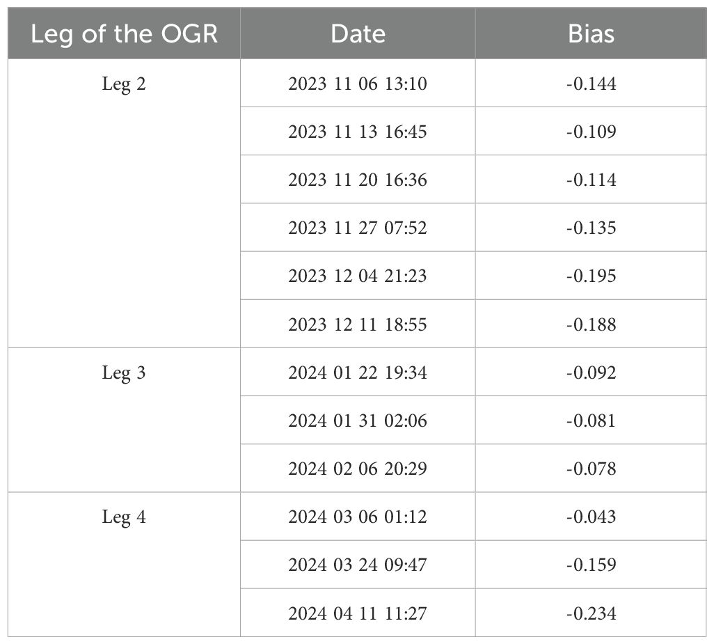
Table 3. Differences between sensor data and salinity references obtained by sampling at control points during the PenDuick VI cruise.

4 Results

In this section, the results of the work are presented, both in terms of methodology performance and oceanographic data. Firstly, the denoising process is discussed, showing the algorithm behavior on a sample dataset; secondly, the denoising results are presented for Legs 2, 3, and 4; thirdly, the bias analysis and correction are discussed; and lastly, the final data output is presented and analyzed.

4.1 Data filtering performance

This subsection considers a data sample with noise episodes from Leg 4, ranging from 2 April 2024, 10:25 to 3 April 2024, 03:46 (UTC times and one measure per minute). The following figures show the denoising process for both temperature and salinity, considering the aforementioned time interval and a “zoom in”, ranging from 2 April 2024, 21:45 to 3 April 2024, 01:27. Salinity data correspond to the practical salinity calculated from temperature and conductivity data according to the PSS-78 scale.

Figure 3 shows on the left part of the interval an episode of measurements where the noise is little enough not to trigger quality controls greater than 1. As noise appears in the signal, it is shown how those points that differ significantly from the WD or the AD denoise lines are labeled with greater QC values. In this figure, most of them remain probably good data (QC=2, in green) and some are labeled as probably bad data (QC=3, in pink).

Figure 3

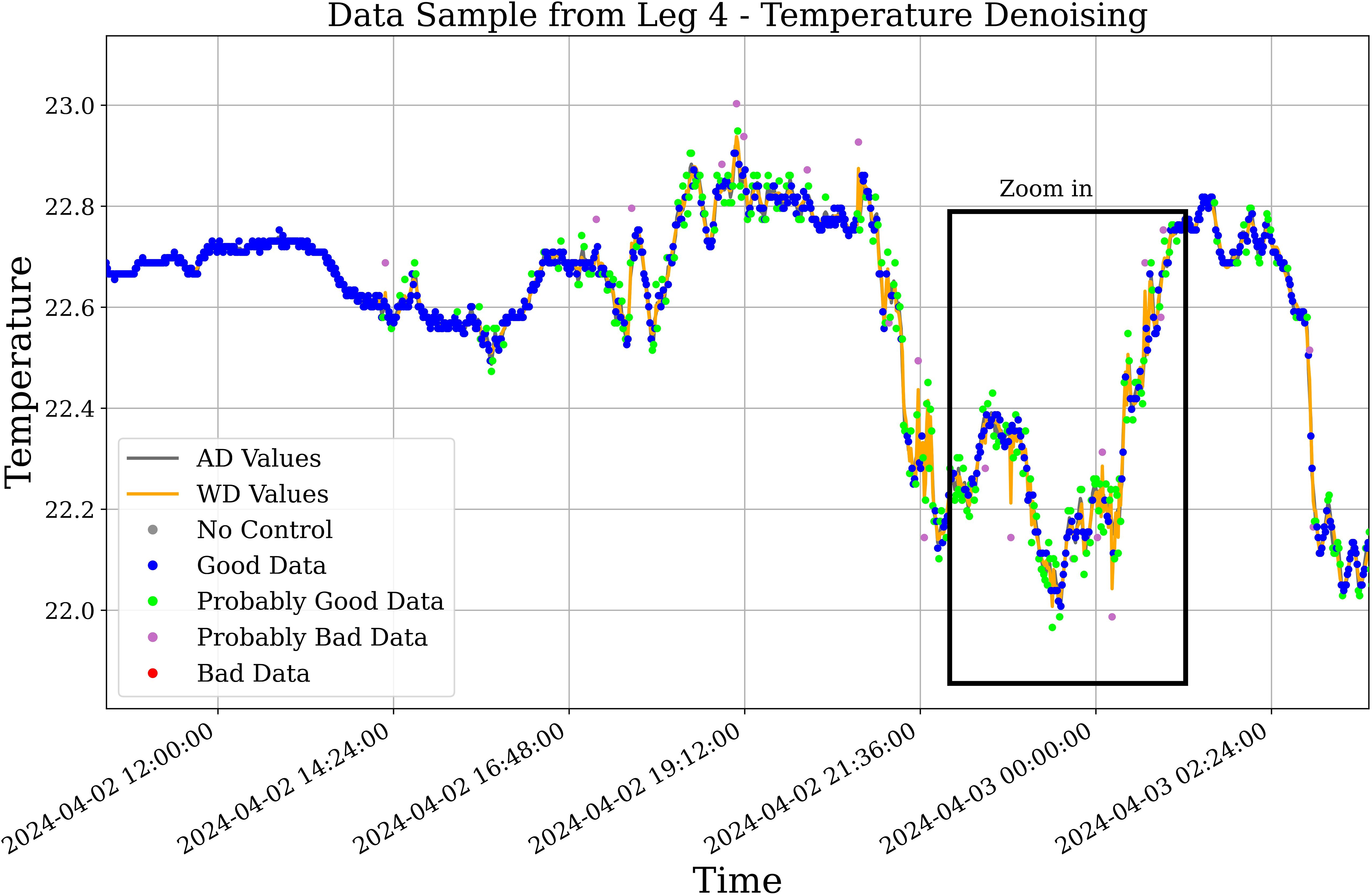
Figure 3. Denoising process on a temperature data sample with noisy episodes from leg 4. WD values are shown in orange. AD values after one iteration are plotted in gray, but are hidden beneath the WD line, see Figure 4 for a better visualization.

With one iteration of AD, the algorithm follows these filtering steps: (a) the WD values are computed, (b) these values are compared to the original data and QC labels are set, (c) AD values are computed for points that still satisfy QC< 3, and (d) these values are compared to the original data again and QC labels are set in a non-decreasing way. Recall that thresholds in use for temperature are [t₁,t₂,t₃] = [0.02,0.05,0.1] (°C).

Figure 4 presents a narrow window of time from this same data sample to better show the denoised values. The plot illustrates how the WD values have a higher tendency to reach the outliers than the AD values, as mentioned in Subsection 3.1. However, in the combination of both denoising methods, close to manual performance is achieved in filtering outliers.

Figure 4

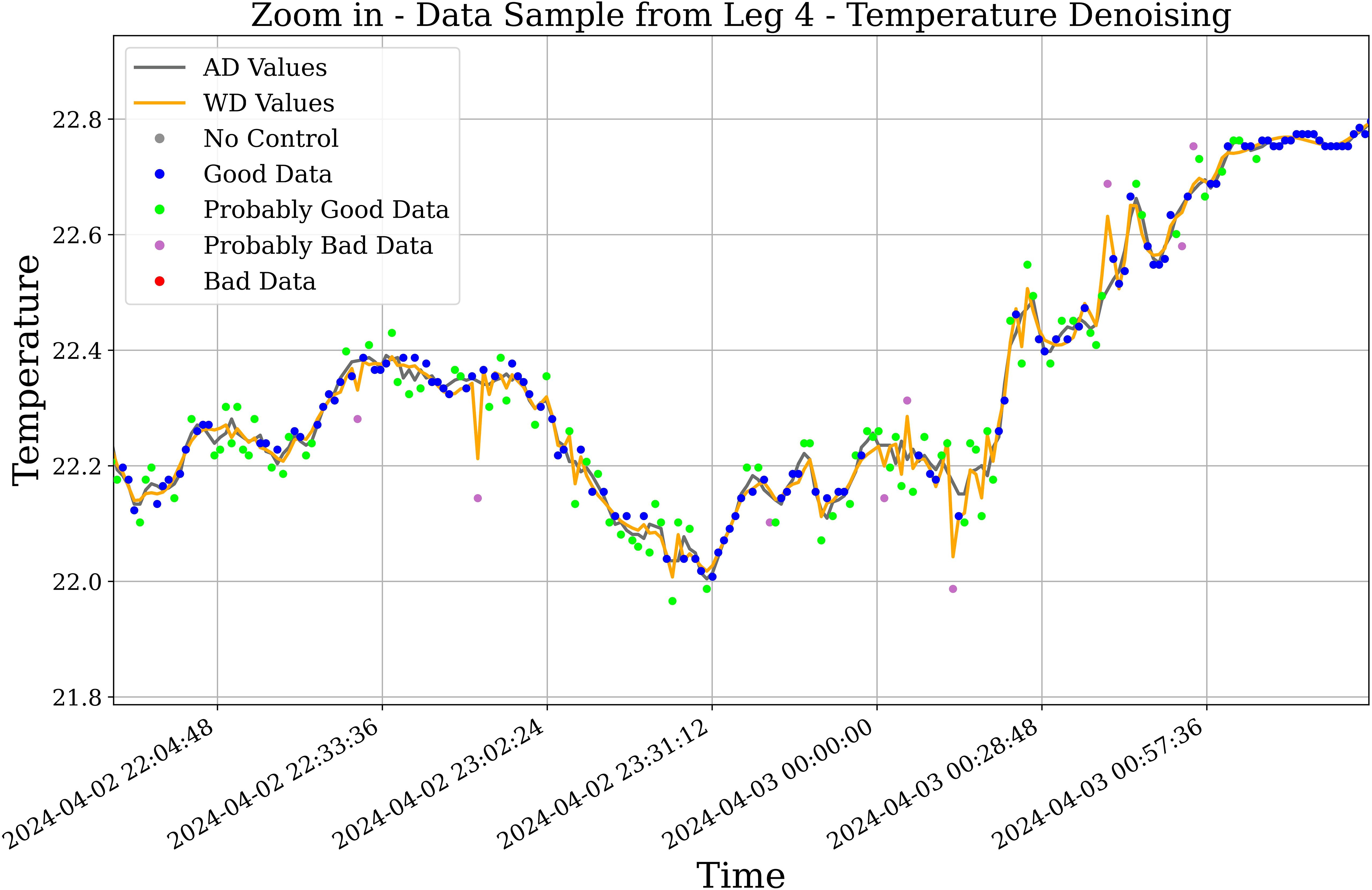
Figure 4. Zoom in from Figure 3. Denoising process on a temperature data sample with noisy episodes from leg 4. WD values are shown in orange and AD values after one iteration are shown in gray.

In Figure 5, we present the corresponding salinity data of the time interval from Figure 3 (temperature). The downwards spikes show a typical noisy behavior of this sort of salinity data Umbert et al. (2022), which is successfully filtered by the algorithm, as these points are labeled with QC = 3 (pink) or QC = 4 (red). Recall that thresholds in use for salinity are [t₁,t₂,t₃] = [0.007,0.015,0.05]. Note that some of these distant outliers are being labeled as probably bad, even when they fall far apart from the main signal feature. This can be easily addressed by shifting t₃ toward t₂. However, being t₂ the most relevant threshold to the study, it was chosen not to do so in order to better show the behavior of the algorithm.

Figure 5

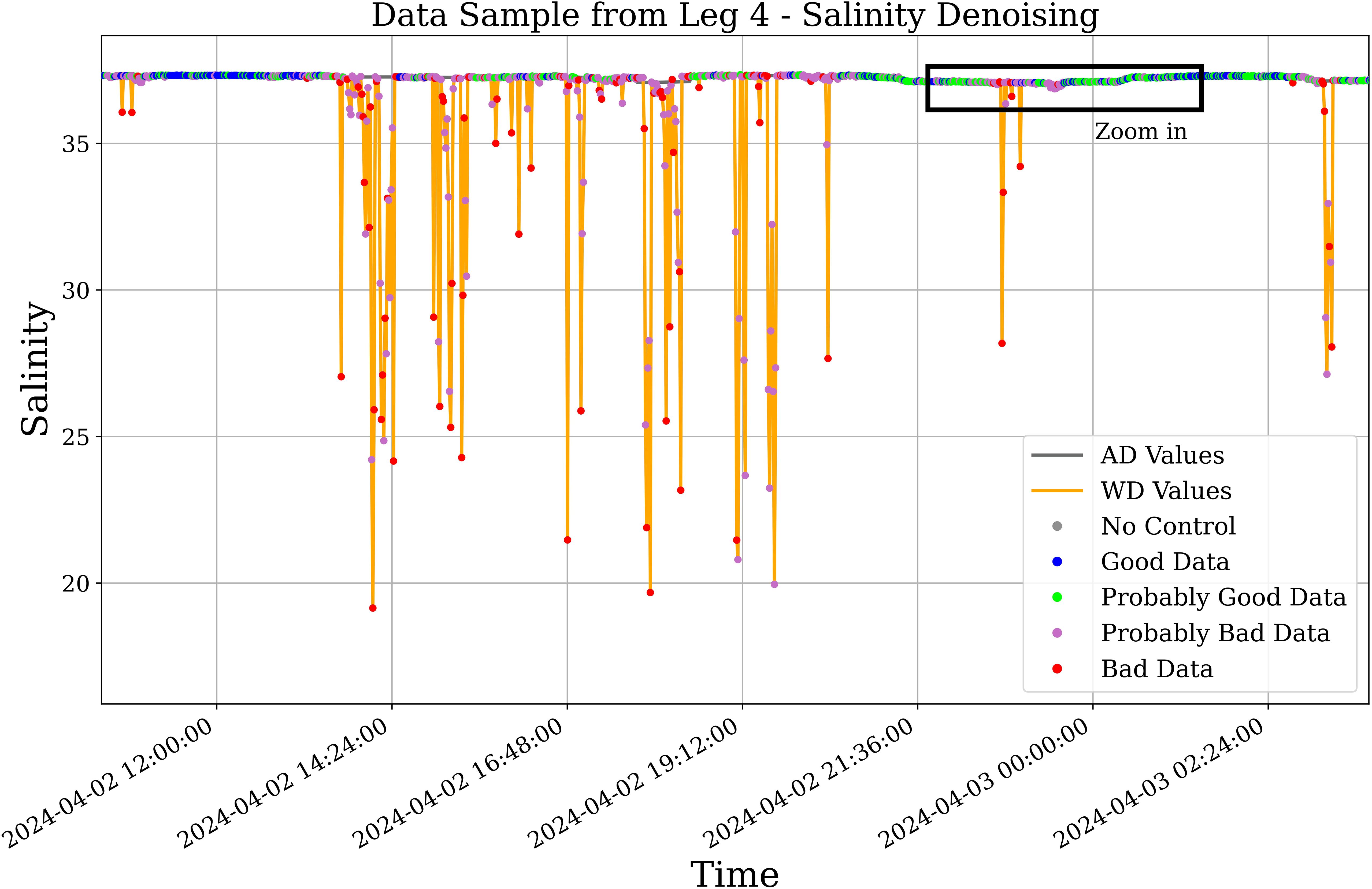
Figure 5. Denoising process on a salinity data sample with noisy episodes from leg 4 corresponding to Figure 3 time interval. WD values are shown in orange, and AD values after two iterations are shown in gray. The downward spikes are characteristic of this type of data, typically caused by air bubbles going through the conductivity sensor.

Also recall that in the case of salinity, two rounds of AD were needed, resulting in the following steps of processing: (a) the WD values are computed, (b) these values are compared to the original data and QC labels are set, (c) AD values are computed for points with QC< 3 (first round of AD), (d) these values are compared to the original data and QC labels are set in a non-decreasing way, (e) AD values are produced with the remaining data with QC< 3 (second round of AD), and (f) these values (from second AD round) are compared to the original data and QC labels are set in a non-decreasing way.

The plots for salinity are shown as AD values, the ones resulting from the second round of AD denoising together with those points that were involved in round 1 but not in round 2, that is, the points that were already labeled as “bad” or “probably bad” in round 1.

Figure 6 presents salinity data on the same time window as Figure 4. It provides a clear example of how WD tends to reach distant outliers. The plot also shows how the presence of such an outlier induces oscillation on the surrounding WD values. Therefore, even if a high percentage of these points is still being labeled as “bad” or “probably bad” through WD, AD has shown to be valuable in cleaning the remaining outliers.

Figure 6

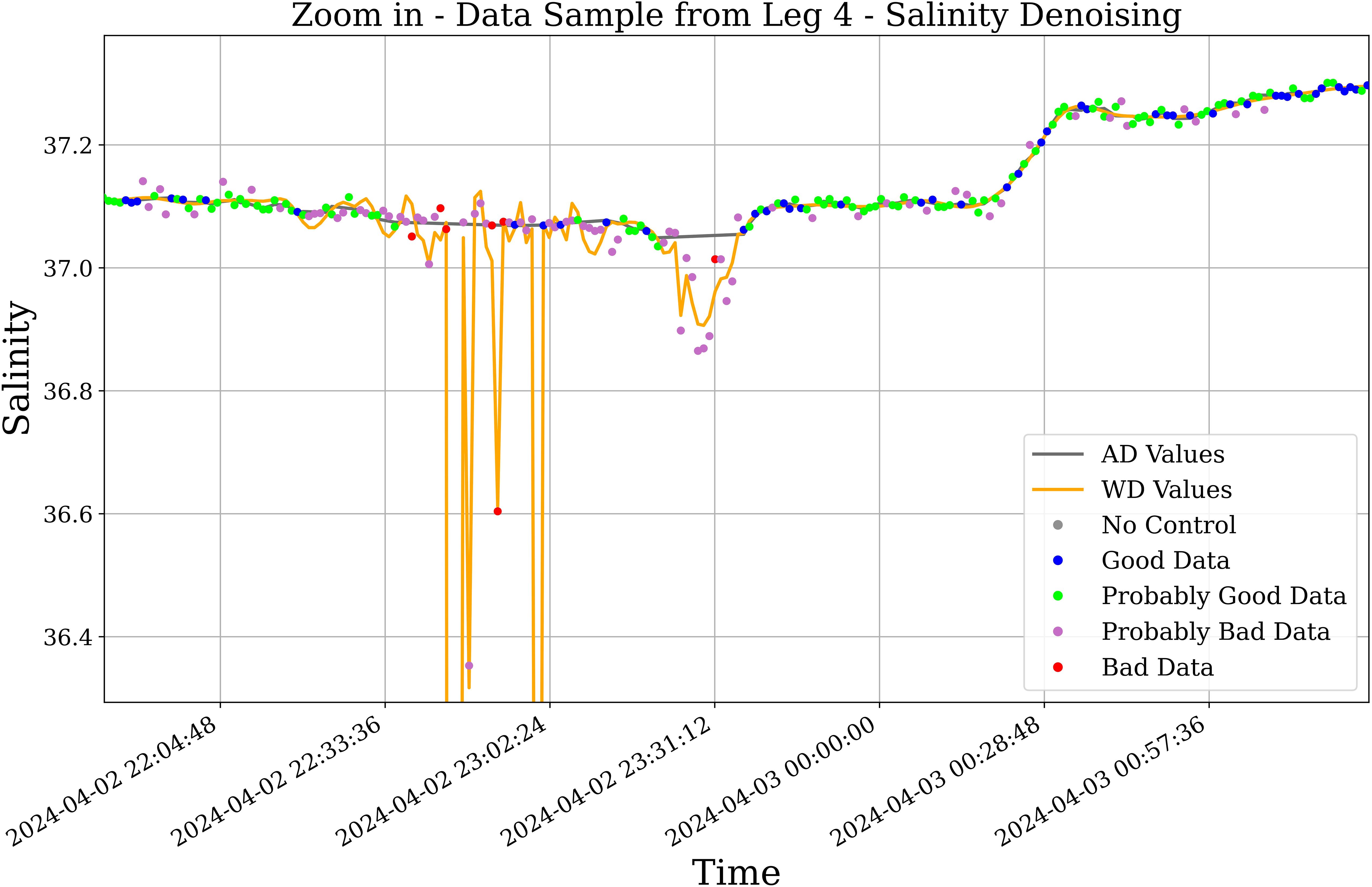
Figure 6. Zoom in from Figure 5. Denoising process on a salinity data sample with noisy episodes from leg 4. WD values are shown in orange, and AD values after two iterations are shown in gray.

4.2 Data filtering on Legs 2, 3, and 4

This subsection presents a set of figures showing a global view of how the algorithm worked on Legs 2, 3, and 4 (Figures 7–13). The thresholds that were used are presented together with the percentages of each quality flag.

Figure 7

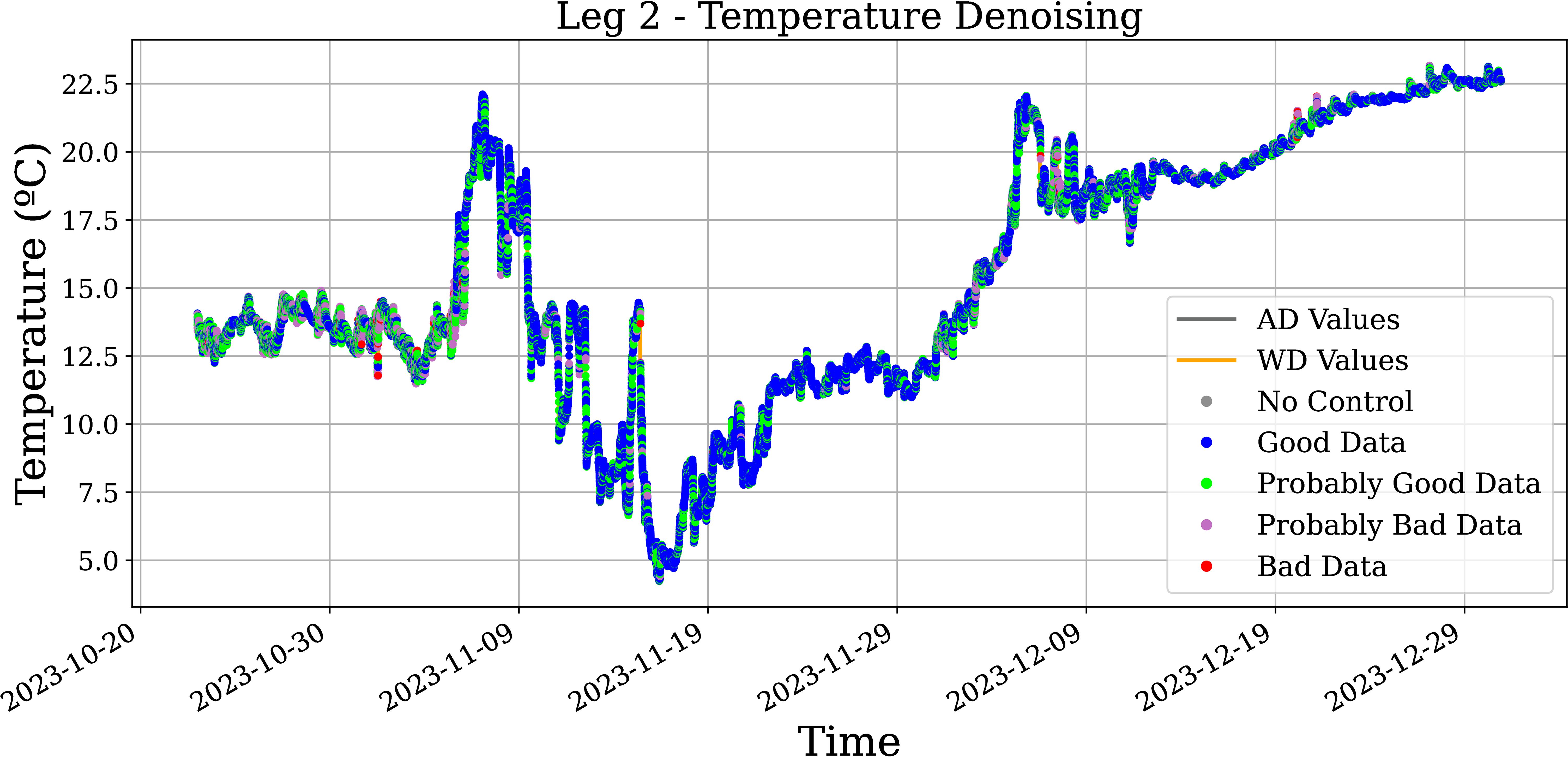
Figure 7. Temperature data during Leg 2 of the race, with WD and AD filtering applied. The table shows the settings of the filtering method and the percentages of quality control labels in the output.

Figure 8

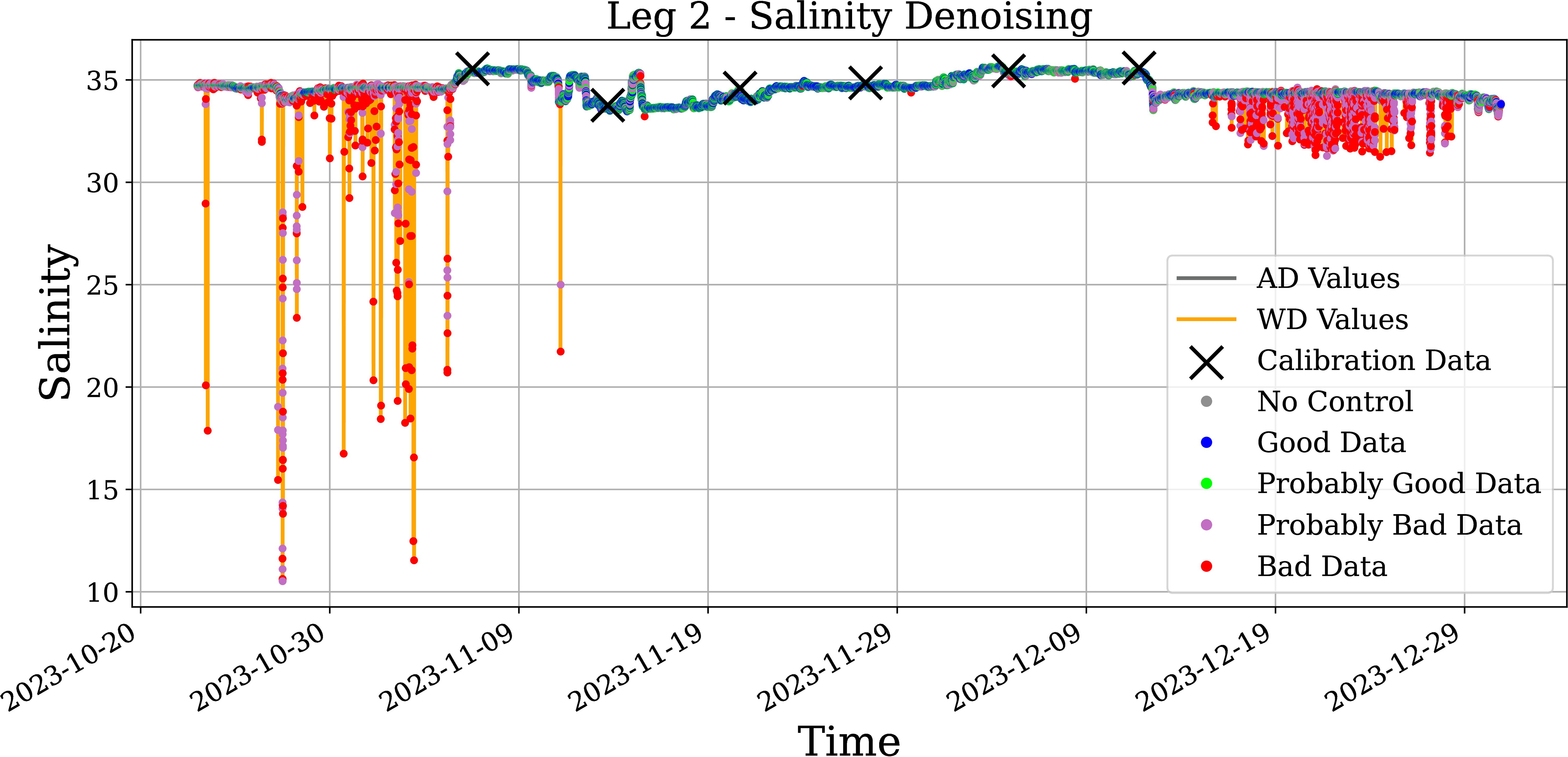
Figure 8. Salinity data during Leg 2 of the race, with WD and AD filtering applied. The table shows the settings of the filtering method and the percentages of quality control labels in the output.

Figure 9

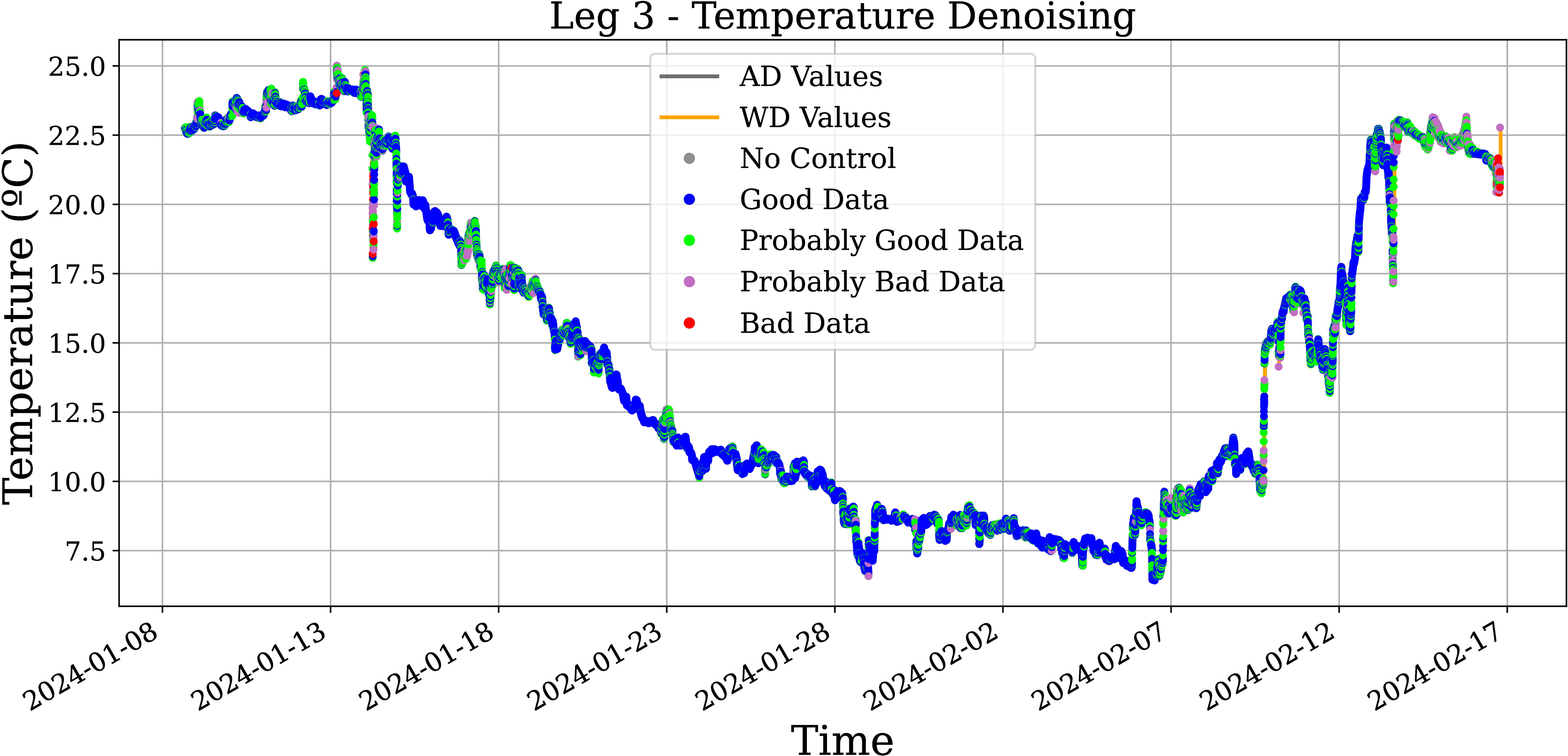
Figure 9. Temperature data during Leg 3 of the race, with WD and AD filtering applied. The table shows the settings of the filtering method and the percentages of quality control labels in the output.

Figure 10

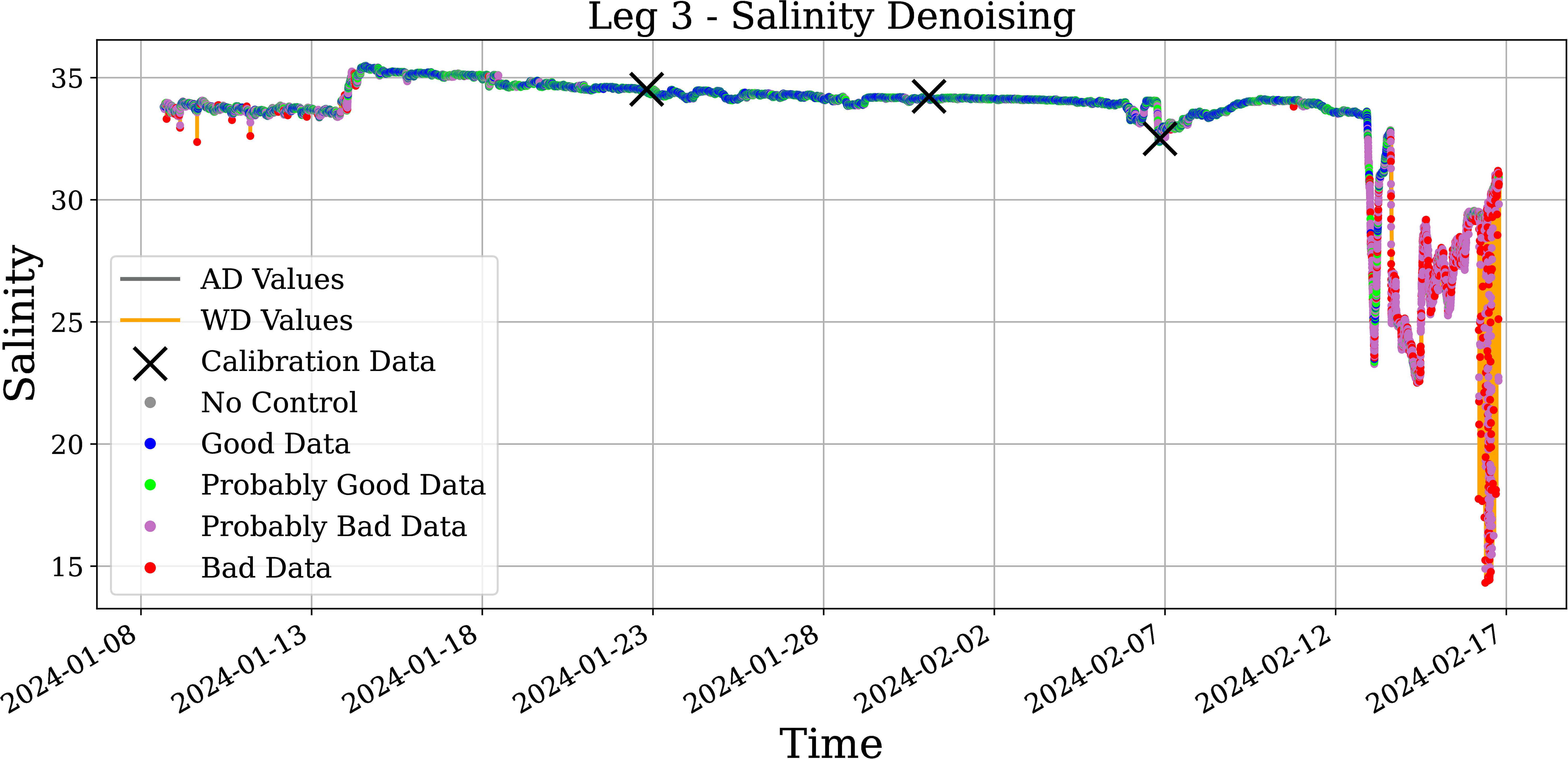
Figure 10. Salinity data during Leg 3 of the race, with WD and AD filtering applied. The table shows the settings of the filtering method and the percentages of quality control labels in the output.

Figure 11

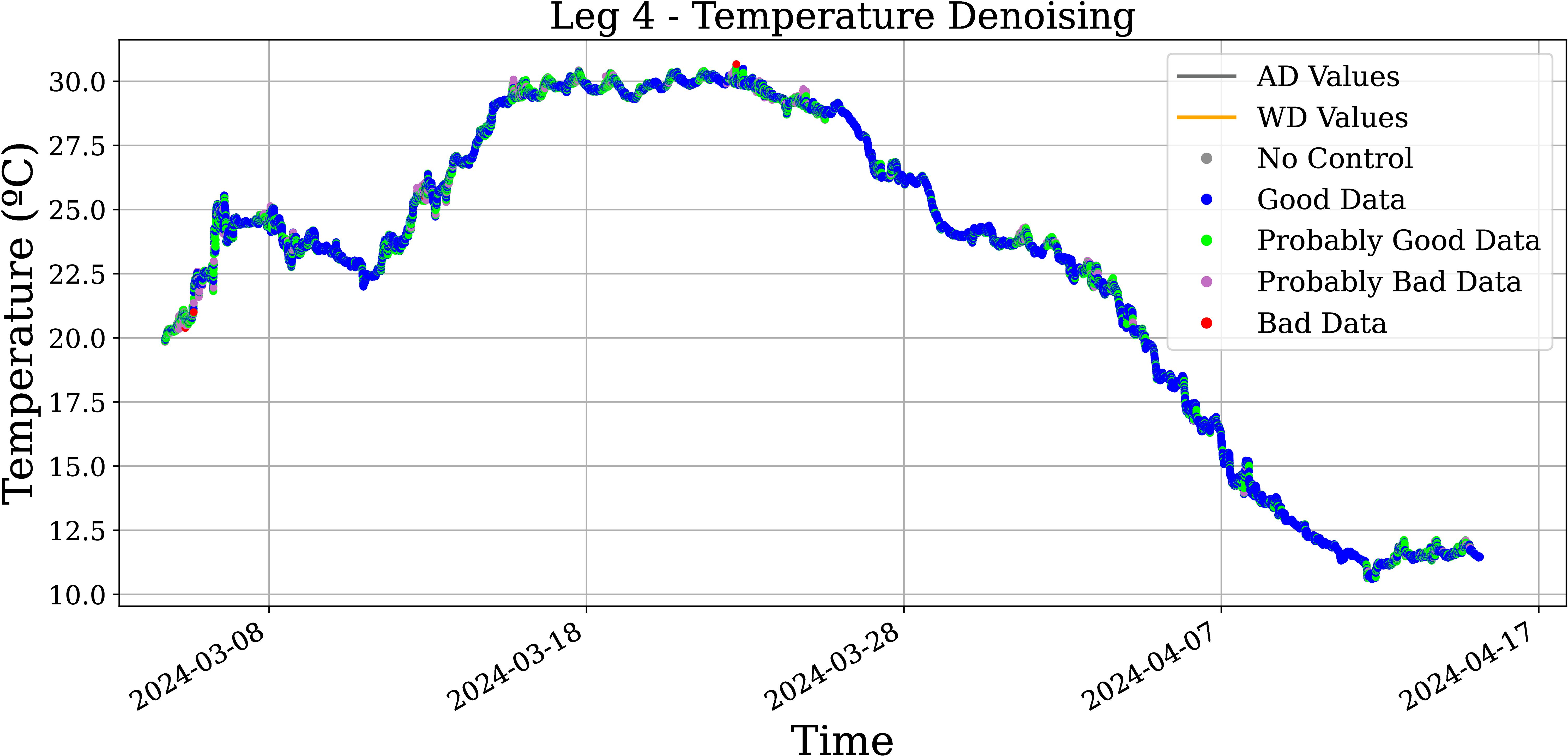
Figure 11. Temperature data during Leg 4 of the race, with WD and AD filtering applied. The table shows the settings of the filtering method and the percentages of quality control labels in the output.

Figure 12

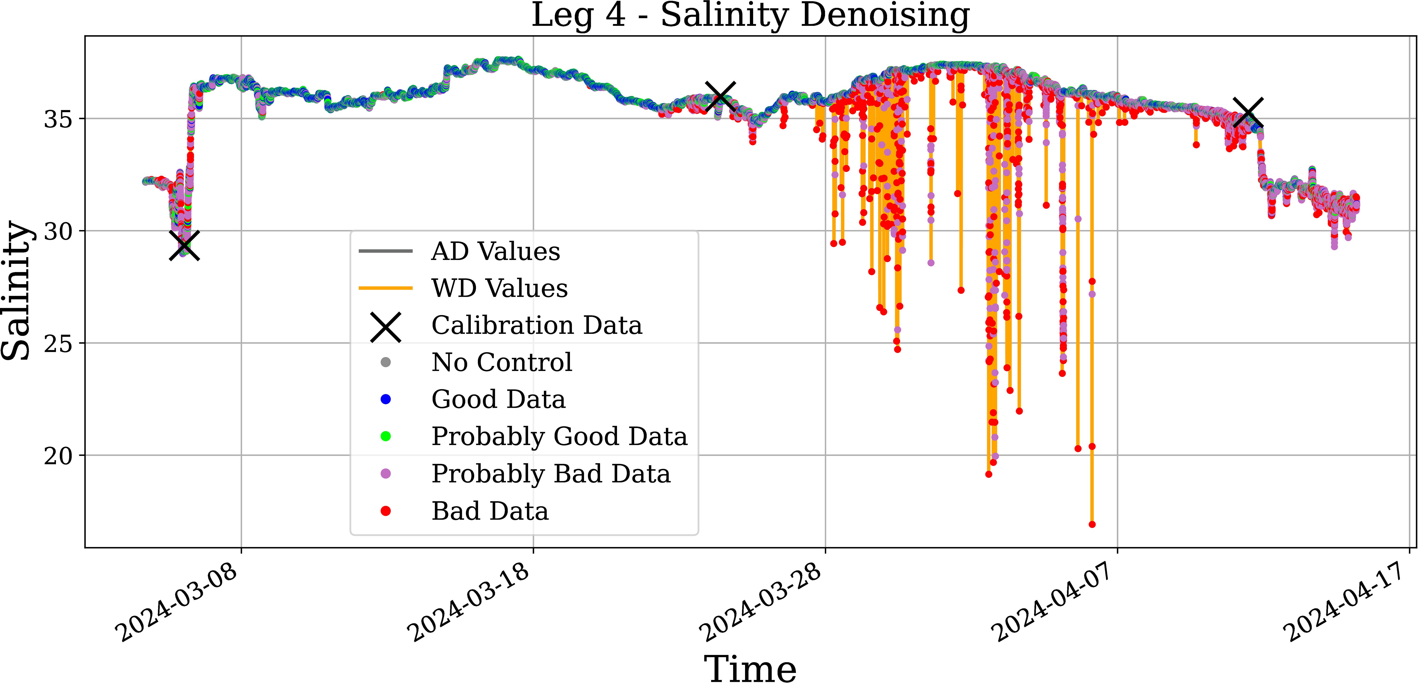
Figure 12. Salinity data during Leg 4 of the race, with WD and AD filtering applied. The table shows the settings of the filtering method and the percentages of quality control labels in the output.

Figure 13

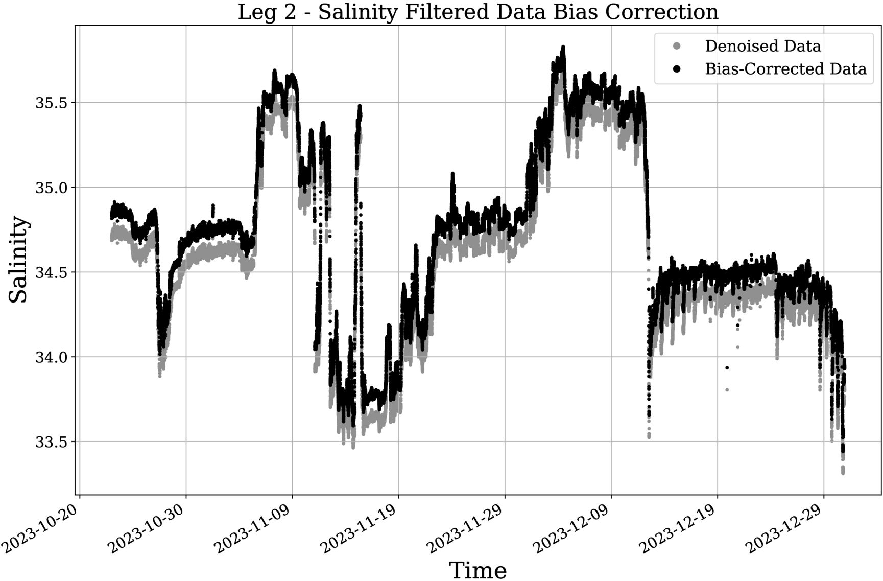
Figure 13. Leg 2 filtered data from denoising (gray) and final data (black) with a +0.130 bias correction.

4.3 Salinity bias analysis

Table 3 shows the resulting biases from water samples for all Legs. It also shows how the sensor was under-measuring salinity at all times, recording the less biased results in Leg 3 and showing the greatest bias value -in absolute terms- at the end of Leg 4.

As described in subsection 3.2, the bias is taken as the mean value from Table 3, which is −0.127. Imposing a 95% confidence, an imprecision of 0.115 is obtained for this value. Therefore, all salinity data are to be shifted +0.13 and to be considered with ±0.1 precision.

4.4 Oceanographic observations

The filtered sea surface salinity and temperature (Figure 14) maps reveal distinct hydrographic structures as the vessel navigates the Subantarctic Zone during Legs 2 and 3. South of 40°S, along the path of the Antarctic Circumpolar Current, clear gradients in both T and S are observed, especially in the Pacific and Indian sectors.

Figure 14

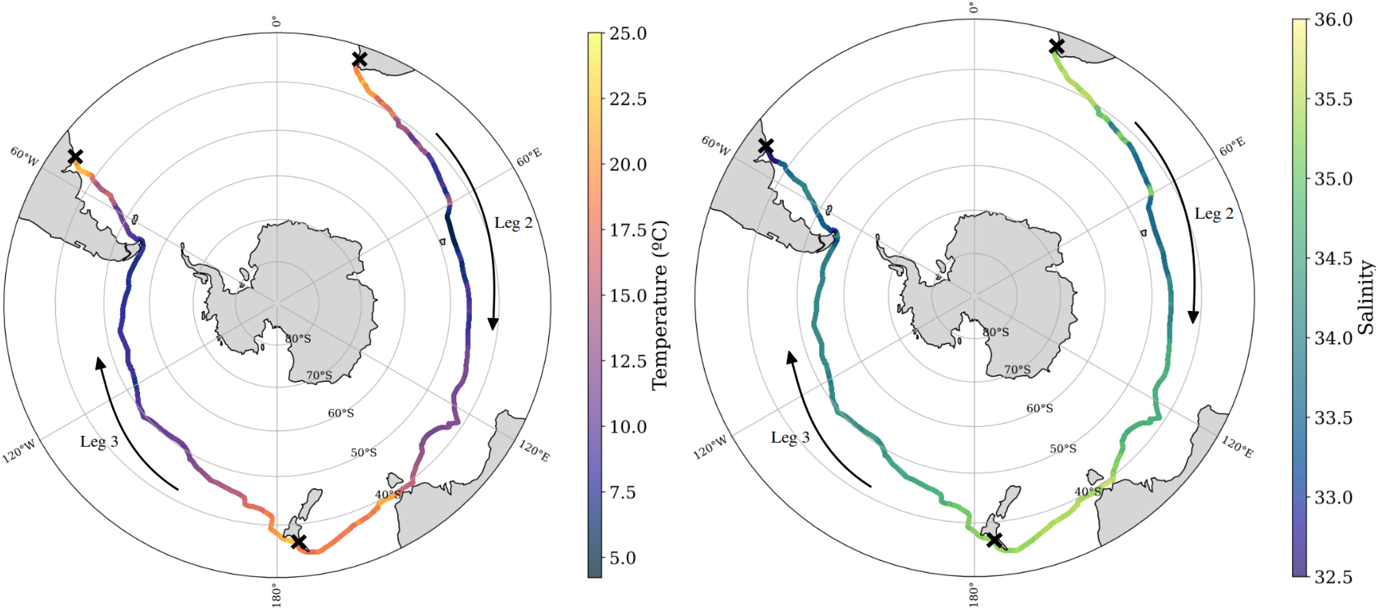
Figure 14. Temperature (left) and salinity (right) along Leg 2 (Nov 5 – Dec 28, 2023) and Leg 3 (Jan 14 – Feb 27, 2024).

Salinity values range from approximately 33.5 to 35.5, showing a freshening trend near 50–60°S (likely due to Antarctic surface waters and precipitation influence) and increasing sharply north of the Subantarctic Front (SAF), where subtropical waters dominate Chapman et al. (2020). The temperature distribution follows a similar pattern, with colder waters (5–10°C) near 60°S and warmer values (up to 20°C) closer to 40°S, marking the transition across the SAF and Subtropical Front (STF).

The temperature (left panel; Figure 15) and salinity (right panel; Figure 15) distributions along leg 4 reveal a clear latitudinal gradient consistent with large-scale oceanographic structures in the Atlantic Ocean.

Figure 15

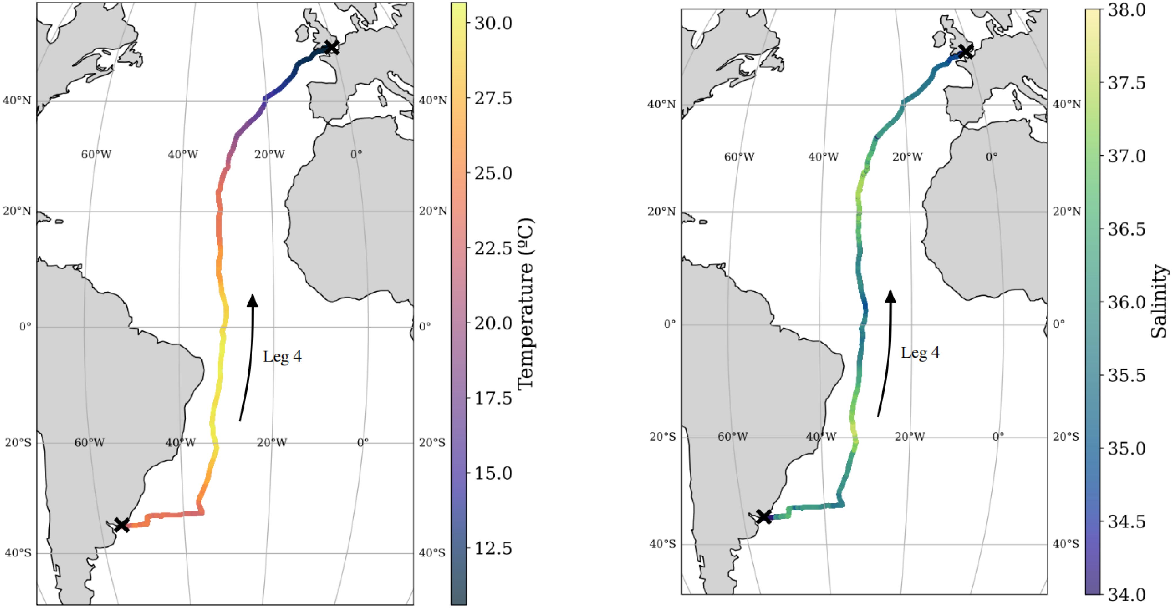
Figure 15. Temperature (left) and salinity (right) along Leg 4 (Mar 5 – Apr 16, 2024).

Surface temperature ranges from approximately 11.5°C in the north (near 40°N) to over 30°C in the tropics, reflecting the transition from temperate waters of the North Atlantic to the equatorial warm pool. Salinity, in turn, ranges from about 34 to 38, with the highest values located between 10°N and 30°N, associated with Subtropical Surface Waters, where evaporation exceeds precipitation. Fresher waters are observed near the equator and south of 20°S, possibly influenced by river outflow or rainfall.

5 Discussion

Traditional approaches to filtering sea surface temperature and salinity data collected from vessel-based platforms often rely on threshold-based criteria or simple statistical techniques to identify and remove outliers [e.g., Bushnell et al. (2019); U.S. Integrated Ocean Observing System (IOOS) (2020)]. While these methods can be effective in removing gross errors due to bubbles, water stagnation, or sensor lags, they often lack adaptability in dynamic ocean environments and may fail to capture more subtle, transient anomalies. In this study, we proposed an automated filtering method that builds on these classical approaches but incorporates a more robust and systematic framework to improve data quality, particularly in the challenging context of data collected from racing yachts.

In this study, we have gone beyond conventional filtering by incorporating methodologies drawn from image processing, specifically wavelet-based denoising techniques applied in one dimension [e.g., Merry (2005); Truchetet (1998)]. These methods, which are particularly effective at isolating multi-scale structures, allowed us to better capture the fine-scale variability in SST and SSS time series while minimizing the influence of instrumental noise.

While the proposed automated filtering method successfully improves data quality by mitigating noise caused by bubble formation and water stagnation, certain limitations remain. The algorithm relies on predefined thresholds and statistical techniques that may not fully adapt to highly dynamic oceanic conditions, particularly under relatively low measurement frequencies. In extreme weather events or regions with strong currents, transient anomalies in temperature and salinity could still be misclassified as noise if the measuring frequency is not high enough, potentially leading to data loss. Additionally, the method assumes uniform sensor performance across different vessel speeds and sea states, which may not always hold true. Future refinements should incorporate adaptive filtering techniques that dynamically adjust to environmental variability, improving robustness in challenging conditions.

The filtering approach developed in this study has the potential to be applied beyond the Ocean Globe Race dataset. Similar denoising methodologies could enhance data quality in other vessel-based oceanographic programs, such as ferry-based monitoring networks, autonomous surface vehicles, and research cruises. The technique could also be adapted for use in low-cost sensor deployments on commercial ships, expanding data collection capabilities in under-sampled ocean regions. By refining and validating this approach across multiple platforms, the method could contribute to the standardization of automated filtering procedures for vessels of opportunity within global ocean observing networks.

The ability to obtain high-quality in-situ SST and SSS measurements from non-traditional observation platforms has significant implications for oceanographic research. Improved datasets contribute to better calibration and validation of satellite-derived products, reducing uncertainties in global climate monitoring. Additionally, high-resolution data from racing yachts provide new insights into small-scale ocean processes, including sub-mesoscale eddies and boundary layer interactions, which are often underrepresented in coarse-resolution climate models. The development of automated filtering techniques also supports the broader effort to integrate machine learning and artificial intelligence into oceanographic data processing, paving the way for more efficient and scalable ocean monitoring solutions.

6 Conclusion

The present study presents a robust and systematic method to filter SST and SSS data collected from vessels of opportunity, particularly in the demanding conditions of ocean racing. By integrating wavelet-based denoising techniques, the approach effectively reduces noise while preserving fine-scale oceanographic variability.

The method presented in this manuscript advances the field by showing that automated data denoising techniques can achieve manual-level performance while significantly improving processing speed. The system is more efficient because it reduces costs and provides similar filtering standards. Although some limitations remain under particular conditions, the method offers a valuable step toward standardized, automated processing of in-situ ocean data.

Its potential application across diverse platforms highlights its relevance for enhancing global ocean observing systems and improving the validation of satellite products. The continued refinement and expansion of these methodologies will enhance observational capacity in climate-sensitive and remote ocean regions, strengthening global efforts to monitor the changing global ocean.

Data availability statement

The datasets generated and analyzed in this study are available at https://doi.org/10.20350/digitalCSIC/17202. The source code used for data processing and denoising is available at https://doi.org/10.20350/digitalCSIC/17203 (see the README file).

Author contributions

NW-P: Software, Investigation, Writing – review & editing, Writing – original draft, Formal analysis, Resources, Visualization, Methodology, Data curation, Validation, Supervision, Conceptualization, Project administration. OC-S: Investigation, Resources, Writing – review & editing, Writing – original draft, Methodology, Conceptualization. MU: Writing – review & editing, Funding acquisition, Conceptualization, Investigation, Writing – original draft, Supervision, Resources, Validation, Visualization, Project administration, Methodology. NH: Visualization, Resources, Writing – original draft, Project administration, Conceptualization, Validation, Data curation, Investigation, Writing – review & editing, Supervision. JS: Writing – review & editing, Supervision, Writing – original draft, Formal analysis, Conceptualization, Validation. TR: Conceptualization, Writing – original draft, Methodology, Data curation, Investigation, Funding acquisition, Resources, Writing – review & editing, Project administration.

Funding

The author(s) declare that financial support was received for the research and/or publication of this article. N. Werner and M. Umbert are funded by the ERC-2024-StG FRESH-CARE (Grant Agreement: 101164517). O. Carrasco-Serra is funded by the grant FPU-UPC, from the Universitat Politècnica de Catalunya with the collaboration of Banco de Santander. This work was supported by grant CEX2024-001494-S, funded by AEI (10.13039/501100011033).

Acknowledgments

Our sincere thanks go to Marie Tabarly for offering us the opportunity to mount the sensor on Pen Duick VI’s keel, and to Arnaud Pennarun for his skilled craftsmanship in attaching and painting the sensor housing. We gratefully acknowledge Eng. Pol Umbert for procuring and delivering the sampling flasks to the vessel in Cape Town, which made it possible to collect water samples for the correction of salinity data. We also thank Gerard Martinez for his contribution in 3D printing the sensor housing. We extend our appreciation to Eloїse Le Bras, Julia Joly, and Tom Napper, members of the crew, for their commitment to collecting salinity water samples and for diligently maintaining the NKE sensor throughout the entire regatta.

Conflict of interest

The authors declare that the research was conducted in the absence of any commercial or financial relationships that could be construed as a potential conflict of interest.

The handling editor FM declared a past co-authorship with the author MU.

Generative AI statement

The author(s) declare that no Generative AI was used in the creation of this manuscript.

Publisher’s note

All claims expressed in this article are solely those of the authors and do not necessarily represent those of their affiliated organizations, or those of the publisher, the editors and the reviewers. Any product that may be evaluated in this article, or claim that may be made by its manufacturer, is not guaranteed or endorsed by the publisher.

Supplementary material

The Supplementary Material for this article can be found online at: https://www.frontiersin.org/articles/10.3389/fmars.2025.1602092/full#supplementary-material

Footnotes

1. ^ Harbour data are typically identified based on vessel speed and may be valuable for analysis; however, this aspect is not addressed in the present study.

References

Addison P. S. (2002). The illustrated wavelet transform handbook: introductory theory and applications in science, engineering, medicine and finance (New York: Taylor & Francis). doi: 10.1201/9781420033397

Crossref Full Text | Google Scholar

Behncke J., Landschützer P., and Tanhua T. (2024). enA detectable change in the air-sea CO2 flux estimate from sailboat measurements. Sci. Rep. 14, 3345. doi: 10.1038/s41598-024-53159-0

PubMed Abstract | Crossref Full Text | Google Scholar

Bushnell M., Waldmann C., Seitz S., Buckley E., Tamburri M., Hermes J., et al. (2019). enQuality assurance of oceanographic observations: standards and guidance adopted by an international partnership. Front. Mar. Sci. 6. doi: 10.3389/fmars.2019.00706

Crossref Full Text | Google Scholar

Chapman C. C., Lea M.-A., Meyer A., Sallée J.-B., and Hindell M. (2020). enDefining Southern Ocean fronts and their influence on biological and physical processes in a changing climate. Nat. Climate Change 10, 209–219. doi: 10.1038/s41558-020-0705-4

Crossref Full Text | Google Scholar

Gourrion J., Szekely T., Killick R., Owens B., Reverdin G., and Chapron B. (2020). enImproved statistical method for quality control of hydrographic observations. J. Atmospheric Oceanic Technol. 37, 789–806. doi: 10.1175/JTECH-D-18-0244.1

Crossref Full Text | Google Scholar

Hernani M., Werner-Pelletier N., Umbert M., Hoareau N., Olivé-Abelló A., and Salat J. (2025). enInter-annual hydrographic changes in the Southern Ocean: Analysis of Vendee´ Globe and Barcelona World Race data. (Cambridge, UK: Cambridge University Press).

Google Scholar

Landschützer P., Tanhua T., Behncke J., and Keppler L. (2023). enSailing through the southern seas of air–sea CO2 flux uncertainty. Philos. Trans. R. Soc. A: Mathematical Phys. Eng. Sci. 381, 20220064. doi: 10.1098/rsta.2022.0064

PubMed Abstract | Crossref Full Text | Google Scholar

Merry R. J. E. (2005). englishWa velet theory and applications: a literature study (Eindhoven, The Netherlands: Eindhoven University of Technology).

Google Scholar

Salat J., Umbert Ceresuela M., Ballabrera-Poy J., Fernaádez P., Salvador K., and Martínez J. (2013). enThe Contribution of the Barcelona World Race to improved ocean surface information. A validation of the SMOS remotely sensed salinity. Contributions to Sci. 9, 89–100. doi: 10.2436/20.7010.01.167

Crossref Full Text | Google Scholar

Tanhua T., Gutekunst S. B., and Biastoch A. (2020). enA near-synoptic survey of ocean microplastic concentration along an around-the-world sailing race. PloS One 15, e0243203. doi: 10.1371/journal.pone.0243203

PubMed Abstract | Crossref Full Text | Google Scholar

Truchetet F. (1998). Ondelettes pour le signal numérique, vol. 17 (Paris, France: éditions Hermès, Paris) 156.

Google Scholar

Umbert M., Hoareau N., Salat J., Salvador J., Guimbard S., Olmedo E., et al. (2022). enThe contribution of the vendée globe race to improved ocean surface information: A validation of the remotely sensed salinity in the sub-antarctic zone. J. Mar. Sci. Eng. 10, 1078. doi: 10.3390/jmse10081078

Crossref Full Text | Google Scholar

U.S. Integrated Ocean Observing System (IOOS) (2020). Manual for real-time quality control of in-situ temperature and salinity data version 2.1: a guide to quality control and quality assurance of in-situ temperature and salinity observations (Silver Spring, Maryland, USA: U.S. IOOS Program Office). doi: 10.25923/x02m-m555

Crossref Full Text | Google Scholar