Anomaly detection as vision-based obstacle detection for vehicle automation in industrial environment

1 Introduction

Automated driving on public roads still faces technical and legal challenges. However, on company premises driver-less vehicles already exist. Automated Guided Vehicles (AGV) are able to drive safely by using laser scanners as protective devices. For automating newly produced cars on the company premises of the car manufacturer, it is necessary to use the basic sensor setup for obstacle detection (Wenning et al., 2020). As ultrasonic parking sensors alone do not provide the reliability required for full automation, we look for an additional obstacle detection mechanism. From the year 2022, it will be mandatory to equip all cars with at least a mono camera for the required vehicle functionalities (European Commission, 2019). Thus, automated car logistics on company premises could be realized without additional sensors, if a computer vision algorithm guarantees the required reliability.

Vision-based obstacle detection is an often regarded research area. There have been proposals that use the direct comparison to a reference image (Mukojima, 2016), proposals that use the optical flow (Klappstein, 2008) and many more developments with the rise of deep neural networks. While the classic approaches, that do not use neural networks, lack robustness, many deep-learning based approaches are limited to objects that have been present in the data set used for training. Approaches that generate depth from camera images (Almalioglu et al., 2019; Feng and Gu, 2019) or perform semantic segmentation (Badrinarayanan et al., 2017) require vast amounts of labeled training data, accounting for high development costs.

The use case of factory-automated cars calls for a reliable, vision-based obstacle detection, that can be trained on-site with few training images. This differentiates the task of this paper from the classic automated driving, where large amounts of training data are needed to abstract for complex new situations.

The lower visual complexity on company premises and the well-known vehicle path motivates us to reinterpret the obstacle detection task as an anomaly detection. This approach has the advantage that it can be taught using only the normal environment, which is the path without any obstacles, cf. Figure 1. During operation of the automated vehicle, the algorithm compares the perceived environment to the learned normality model and stops the motion when recognizing any significant deviation. The proposed method makes labeling unnecessary and reduces the amount of training to a fraction. The paper investigates this concept on an application-specific data set.

FIGURE 1

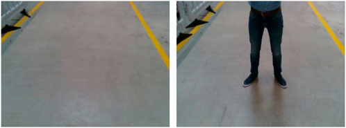
FIGURE 1. Camera view without human obstacle used during training and with human obstacle.

The paper is structured as follows: In the next chapter, we show related work from the field of anomaly detection. Subsequently, we show the classifier design and introduce the data set. Chapter 4 describes the test vehicle and implementation details. After evaluating the approach on the data set in chapter 5, we put it into perpective by comparing the performance to a semantic segmentation. After the summary, future work for a reliable vision-based obstacle detection is discussed.

2 Related work

A wide range of work deals with the task of obstacle detection using only a monocamera. Given the fact that we interpret the task of obstacle detection as anomaly detection (AD), we limit this chapter to current techniques of binary classification with the aim of identifying samples in data that are different from the norm (Chandola et al., 2009), also referred to as novelty, outlier or change detection.

2.1 Learning from scratch

A popular architecture to learn feature representations for an AD task are autoencoders (AE). AE compress input images to a lower embedding and then scale them up to their original dimension, cf. Figure 2. Here, the AE is trained in a semi-supervised manner using only images without anomalies. Anomalous images cannot be reconstructed properly since the algorithm was not confronted with the objects during training. The approach was used in (Bergmann, 2018) and (Haselmann et al., 2018). Following the same idea, (Minematsu et al., 2018), and (Sabokrou et al., 2018) use a Generative Adversarial Network (GAN) instead of an AE.

FIGURE 2

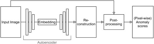
FIGURE 2. AD-architecture using deep autoencoders.

This approach has two drawbacks. The required post-processing increases model complexity, and the decoder part of the AE inherently adds an overhead.

(Andrews et al., 2016; Lawson et al., 2017; Sarafijanovic-Djukic and Davis, 2019) eliminate these downsides by using an AE as a feature extractor in combination with a shallow classifier like a Support Vector Machine (SVM) to classify the learned embedding. Approaches that share the characteristic of this architecture, presented in Figure 3, are called hybrid approaches. In these approaches, the two components are trained independently, but it is also possible to jointly optimize the deep feature extractor and the shallow classifier (Ergen et al., 2017).

FIGURE 3

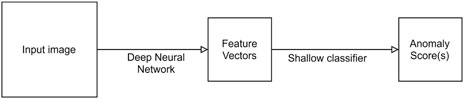
FIGURE 3. General architecture of a deep hybrid approach.

2.2 Transfer learning

Training a deep neural network from scratch requires a large amount of data, which is one of the main disadvantages. In Transfer learning, training data and test data are drawn from a different distribution.

Transfer learning for an AD task can be realized using the deep hybrid approach. A pre-trained deep neural network used as feature extractor is paired with a shallow classifier that is trained in the application domain. Rippel et al. (Rippel et al., 2020) show promising results using the state-of-the-art image classifier EfficientNet (Tan and Le, 2019) trained on ImageNet (Russakovsky et al., 2015). Their approach to use a multivariate Gaussian (MVG) with the Mahalanobis distance as classifier outperforms other methods on an industrial data set. Rippel et al. show that features extracted by EfficientNet that contribute the least to the variance in normal data are highly discriminative in the AD task. Learning these features from scratch would be difficult. Thus, they eliminate the need to train the deep feature extractor by retaining its performance.

Christiansen et al. (2016) firstly use an AD approach as obstacle detection. They analyse different layers of a pre-trained AlexNet (Krizhevsky et al., 2012) and VGG (Simonyan and Zisserman, 2014) as feature extractor in combination with different traditional classification algorithms like Singlevariate Gaussian (SVG), MVG, k-Nearest Neighbour (k-NN) and Gaussian Mixture Models (GMM). They validate the algorithms in the application of an autonomous vehicle in an agricultural environment.

Their work DeepAnomaly implies that good results are possible using a moving camera, including all the difficulties like changing dynamic backgrounds and motion blur. Christiansen et al., however, evaluate their model on a mostly uniform grassland, which is visually not as complex and cluttered as the inside of a factory.

Another interesting approach using a hybrid AD model with a pre-trained feature extractor is presented by Bouindour et al. (Bouindour et al., 2019). They try to detect anomalous motion using a static surveillance camera. Therefore, the neural network C3D extracts spatiotemporal features. The shallow classification used by Bouindour et al. is a so-called balanced distribution (BD) that was purpose-built for the task of distinguishing real anomalies from rare normal events. Here, a sample is only added to the balanced distribution if its Mahalanobis distance is above a certain threshold. The downsides of the balanced distribution in comparison to a simple Gaussian distribution is the increased computation time necessary to construct it, especially when considering large training data sets.

Table 1 sums up the key features of the related work. The obstacle detection for vehicle automation in industrial environments is characterized by a moving camera and an inhomogeneous background. Moreover it needs a state-of-the-art feature extractor and anomaly model.

TABLE 1

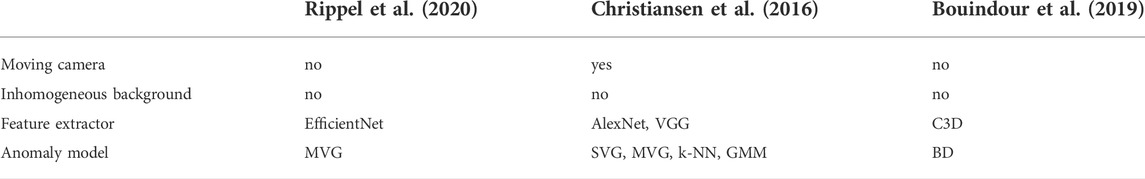
TABLE 1. Key features of related work.

2.3 Need for research

A deep hybrid anomaly detection seems to be a promising approach for obstacle detection. Christiansen et al. show this in an agricultural setting using rather outdated neural networks as feature extractor. Considering the exceptional results using a pre-trained state-of-the-art deep neural network (Rippel et al., 2020), it seems possible to apply the anomaly detection approach in the more complex factory environment. The balanced distribution suggested by Bouindour et al. could further increase the performance.To this end, we test the deep hybrid anomaly detection approach on an application-specific data set, that has not been addressed before. It combines the moving camera with the inhomogeneous factory background. Besides providing the proof of concept as an obstacle detection in factory automation, we test state-of-the-art feature extractors, MobileNet and ResNet, which have not been used in related work yet. Moreover, we compare anomaly models from the related work, SVG and MVG, with the Balanced Distribution from Bouindour et al.. The best performing combination is analysed regarding its reliability in the application.

3 Methods

This paper’s research goal is to test the anomaly detection approach in the use case of vehicle automation in industrial environments. Therefore, we make use of latest anomaly detection components, that are described in this section. Following requirements can be derived from the use case:

• Safety: According to relevant safety standards, the obstacle detection’s failure rate p shall be 10^–7 < p < 10^–6 per hour. (Wenning et al., 2020).

• Robustness: To assure an economic operation the false detection rate should be less than 10^–4 per hour.

• Performance: The obstacle detection must run in real time on standard vehicle computing hardware. Since the computing performance significantly depends on the implementation on special-purpose hardware, it is not analyzed in this paper.

• Velocity: The vehicle drives with 1 m/s. Similarly to AGVs, this corresponds to a safety zone of 1–2 m in front of the car. The algorithm must detect the obstacle in this distance to have sufficient time to stop the car.

• Economy: Automating the addressed use case generates a single-digit profit (€). This implies on the one hand that no additional hardware can be used, which is the motivation to use the monocamera. On the other hand, it requires low development costs. Therefore, we set up the requirement that the anomaly detection shall be trained in a one-time trip of the vehicle.

3.1 Classifier design

In this paper, we will follow the method of a deep hybrid anomaly detection. Figure 4 shows the classifier’s architecture consisting of a pre-trained deep neural network used as feature extractor and a shallow classifier referred to as anomaly model.

FIGURE 4

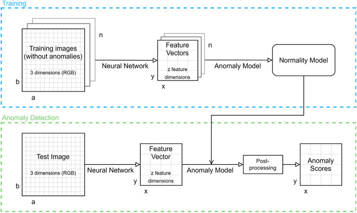
FIGURE 4. General classifier architecture.

During offline training, n anomaly free images with width a and height b are used as input. Depending on the specific neural network, they are transformed into n feature maps consisting of x × y feature vectors with dimension z. These feature vectors are also referred to as patches. The anomaly model will then make use of these feature vectors to create a model of normality.

When testing an input image for an anomaly, the same neural network is applied to extract a feature map. These features are then compared to the normality model resulting in an anomaly score per patch.

The result of comparing the feature map output of the deep neural network with the previously created normality model is an array of anomaly scores of the same dimensions x × y. Due to the stochastic characteristics of neural networks, the output includes noise. It can be eliminated by applying a Gaussian filter with a variance of σ = 1, which blurs the anomaly scores in both image dimensions. The filtered anomaly scores are the algorithms output. By defining a threshold, a binary classification normal/anormal can be derived for each patch.

3.2 Feature extractor

The overview of state-of-the-art methods already showed that deep neural networks can be used as very potent and general feature extractors, even when used in a transfer learning setting for a classification task they were not trained for (Rippel et al., 2020). For this paper, two different deep neural networks at different layers are compared. For better reproducibility, pre-trained network weights are utilized, which are publicly available.

3.2.1 ResNet50V2

Due to their popularity in many different machine learning tasks, different ResNet (He et al., 2016a; He et al., 2016b) variants will also be considered. The ResNet was the first extremely deep neural network architecture that circumvents the problem of vanishing gradients by introducing so-called skip connections. For this paper, the very popular ResNet50V2 is chosen. It consists of 50 layers which are organized in five blocks where the outputs of the last three blocks are examined as feature extractors. Convolutional neural networks are usually tested using the same image resolution, which was also used to train the network. In the case of the ResNet–and many other networks pretrained on ImageNet–this resolution is 224 × 224 pixels. But most deep learning frameworks allow using different resolutions, which simply results in a larger feature map output. This could be useful for more accurately localizing an anomaly. To test this effect, the same ResNet50V2 was used with the intended resolution of 224 × 224 pixels and also 449, ×, 449 pixels.

3.2.2 MobileNetV2

MobileNetV2 (Howard et al., 2017; Sandler et al., 2018) as the name suggests, is a neural network architecture specifically designed to be lightweight enough for execution on mobile devices. Even though the factory use case would theoretically allow handing over the obstacle detection task to a low-latency server (Wenning et al., 2020), fast algorithm that could also run on the vehicle itself is preferred. MobileNetV2 delivers excellent results for ImageNet classification, while still being very fast, and it is a popular choice for mobile computer vision tasks. In total, seven different layers of a MobileNetV2 pre-trained on ImageNet are being examined.

3.3 Anomaly model

The second part of a deep hybrid anomaly detection is a shallow classifier that creates a model of normality in semi-supervised training and then calculates an anomaly score for each new sample. Using this score and a threshold, a sample can be classified as anomalous or normal. Chapter 2.2 already introduced many hybrid AD approaches utilizing different shallow classifiers. Single and multivariate Gaussian showed good results and are therefore used in our application. However, the true distribution of the data in the deep feature space is unknown. The performance of the resulting classifiers give an indication of the extent to which the assumption is fulfilled.

3.3.1 Single variate Gaussian

To create the normality model, the mean and variance for each feature dimension is calculated separately, and correlations between dimensions are not considered. The anomaly measure is then a simplified Mahalanobis distance ${\mathcal{M}}_{\mathit{SVG}}$, which is also sometimes referred to as standardized Euclidean distance.

$\begin{array}{ll}\hfill {\mathcal{N}}_{\mathit{SVG}}\left(x\mid \mu ,{\sigma }^2\right)& =\frac{1}{{\left(2\pi {\sigma }^2\right)}^{1/2}}\exp \left\{-\frac{1}{2{\sigma }^2}{\left(x-\mu \right)}^2\right\}\hfill \\ \hfill {\mathcal{M}}_{\mathit{SVG}}\left(\mathit{x}\mid \mathit{\mu },{\mathit{\sigma }}^2\right)& =\sqrt{\sum _{i=1}^D\frac{{\left(x_i-{\mu }_i\right)}^2}{{{\sigma }_i}^2}}\hfill \end{array}(1)$

3.3.2 Multivariate gaussian

More recent research by (Rippel et al., 2020), however, favors the use of a multivariate Gaussian over a simple SVG in a hybrid AD setting. While they do not consider the computation time, the results obtained using an MVG are significantly superior to an SVG. Creating the MVG is very similar to the SVG, but instead of calculating a separate variance for each feature dimension, one covariance matrix is estimated and the real Mahalanobis distance ${\mathcal{M}}_{\mathit{MVG}}$ is used during anomaly detection.

$\begin{array}{ll}\hfill {\mathcal{N}}_{\mathit{MVG}}\left(\mathit{x}\mid \mathit{\mu },{\mathit{\sigma }}^2\right)& =\frac{1}{{\left(2\pi \right)}^{\frac{D}{2}}|\mathbf{\Sigma }{|}^{\frac{1}{2}}}\exp \left\{-\frac{1}{2}{\left(\mathit{x}-\mathit{\mu }\right)}^T{\mathit{\Sigma }}^{-1}\left(\mathit{x}-\mathit{\mu }\right)\right\}\hfill \\ \hfill {\mathcal{M}}_{\mathit{SVG}}\left(\mathit{x}\mid \mathit{\mu },\mathit{\Sigma }\right)& =\sqrt{{\left(\mathit{x}-\mathit{\mu }\right)}^T{\mathit{\Sigma }}^{-1}\left(\mathit{x}-\mathit{\mu }\right)}\hfill \end{array}(2)$

3.3.3 Balanced distribution

This paper is focusing on the use case of classifying images or image segments into the categories “contains anomaly” or “contains no anomaly”. This wording already indicates that an anomaly is far less common than no anomaly and is thus not represented in the sample data to the same degree. This unequal distribution could result in the wrong classification of rare normal events as anomaly, just because they are rare and not proportionally represented in the normal distribution. To overcome this limitation of a simple Gaussian distribution, a balanced distribution can be used (Bouindour et al., 2019). The balanced distribution is initialized by first selecting N samples from the training data and calculating the parameters for a Gaussian distribution μ and σ². Then, a subsequent sample x is only added to the balanced distribution if its Mahalanobis distance is above a certain threshold α. After adding a sample, the parameters of the Gaussian are recalculated. Having considered each sample in the training data, the balanced distribution is pruned using a threshold η ⋅ α to eliminate redundant elements among the first N samples. Classification is done in the same way, using the Mahalanobis distance of a sample and the balanced distribution to assign it to one of the classes. The algorithm is shown in Figure 5.

FIGURE 5

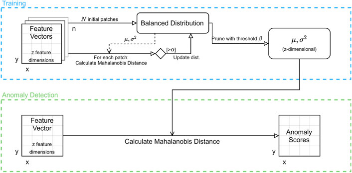
FIGURE 5. Balanced Distribution algorithm for anomaly detection.

Originally, the balanced distribution uses an estimated covariance matrix Σ and the Mahalanobis distance internally, similar to a multivariate Gaussian. To speed up the calculation, we use a simplified version using only the variance σ². Note that this simplification is only used for the decision which patches should be part of the normality model. Our tests have shown that using the faster SVG internally is powerful enough to prevent the grey floor from appearing too often in the modelled data.

In contrast to the single and multivariate Gaussian classifiers, the balanced distribution has three parameters that need to be chosen. In accordance with Bouindour et al., they are selected such that the balanced distribution consists of only 10% of features provided in the training. Using an initial number of N = 500 feature vectors, an empirical assessment showed that this is achieved with a learning threshold α set to the mean of Mahalanobis distances from a simple SVG model combined with a pruning parameter of η = 0.5.

3.4 Labels and metrics

To be able to compare the developed algorithms not only among each other but also to those from the literature, defining different labels and accompanying metrics is necessary, cf. Figure 6.

FIGURE 6

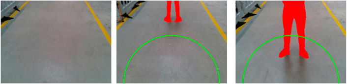
FIGURE 6. Different types of labels: Per-pixel labels in red, per-frame labels using the semicircle: “do not stop” (left), “Not considered in per-frame metric” (middle) and “Stop” (right).

3.4.1 Per-pixel

To evaluate an anomaly detection algorithm in terms of background subtraction, the anomalies in the data set need to be labeled per-pixel. An algorithm will then be judged by its ability to correctly classify each pixel. As the output of a classifier can have a lower resolution than the input image, the labels need to be down-sampled as well such that they match the output resolution of the classifier. Knowing exactly where an anomaly is located within an image is not necessary for the use case but it could enable more sophisticated methods like comparing the location of the obstacle to the planned trajectory and acting accordingly. Taking a look at per-pixel classification also enables a comparison with different background subtraction and per-pixel anomaly detection algorithms from the literature.

3.4.2 Per-frame

The actual output of the classifier should directly signal whether the vehicle needs to stop or not. The two classes the data set needs to be split into is “stop” and “do not stop”. Labeling this quite unspecific criterion is challenging as it requires some judgement by the labeler. To assist in an optimal labeling process, the following criteria are used:

I) Every image with an anomaly in a semicircle covering the bottom half of the image is labeled “stop”. The semicircle corresponds to AGV’s safety zone for obstacle detection.

II) When there is no anomaly in the image, it is labeled “do not stop”.

III) The images that do not fall in either category, for example images with an anomaly outside the semicircle, are not considered in this metric.

4 Implementation

The described AD methods shall be applied to the use case of an obstacle detection in an industrial environment. Publicly available data sets often address the use case of automated driving on public roads. Therefore, we record use case-specific images with a demonstrator vehicle.

4.1 Demonstrator vehicle

We chose Kate small AGV (Schmidt, 2020) as vehicle platform, cf. Figure 7. Laser scanners enable precise localization. A top-mounted aluminum rack holds an Intel RealSense D435 camera at a height of 1.55 m, approximately where windshield cameras are located. The camera’s angle of 35° enables capturing a wide field of floor in front of the vehicle–up to a distance of 6 m. Since the vehicle’s velocity is around 1 m/s, a distance of 1–2 m would be sufficient to trigger the brake in time.

FIGURE 7

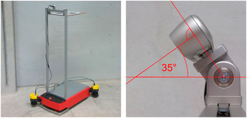
FIGURE 7. Vehicle platform Kate and the mounting of the camera.

4.2 Reference data set

The data set was recorded in the ramp-up factory of RWTH Aachen University. The images contain usual obstacles that can be found in industrial environments, cf. Figure 8. In the training run, certain objects, i.e. barriers, floor markings and barrier chains, can be found at the edge of the path and are then placed as an obstacle on the path during testing. Since the appearance is already known from the training phase, it becomes challenging to detect them as obstacles. The training fraction is recorded in a one-time trip of the vehicle. Thus, the AGV visits each location of the path only once. In the testing phase, roughly the same locations are revisited, making it possible to learn the environment “by heart”.The limited amount of training data, provided in Table 2, reflects the challenge to learn the task of obstacle detection with low costs for labeling and data acquisition.

FIGURE 8

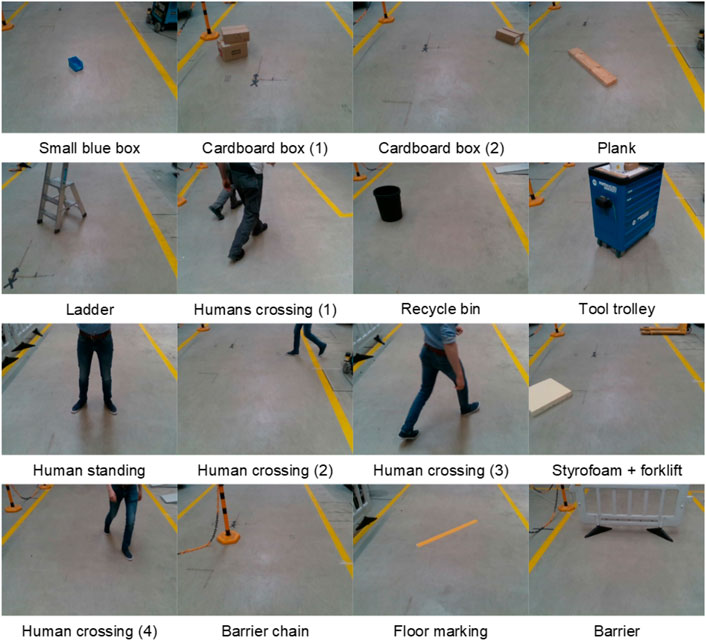
FIGURE 8. Extract from data set showing examples of obstacles in an industrial environment.

TABLE 2

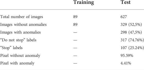
TABLE 2. Data set overview.

4.3 Labels

Different metrics with the accompanying labels were established in chapter 3.4. Per-pixel labels were generated manually at the full image resolution and then down-sampled for each individual deep neural network to match the respective output resolution. Labels for the per-frame metric were also assigned using the full image resolution with the semicircle criterion. Table 2 provides an overview of the data set composition. Training and test data is split such that the training covers the images of only one run down the path without any obstacle.

4.4 Classifier implementation

The deep feature extractors of the hybrid approach were implemented using TensorFlow 2.1. Python and NumPy were used for implementation of the shallow classifier. The neural networks were evaluated on a NVIDIA TITAN Xp graphics card with 12 GB of memory and all other calculations using an Intel Core i7-6850K CPU with 40 GB of RAM. The neural networks use pre-trained weights. The classifier’s configuration is described in Methods and Evaluation Section.

5 Evaluation

The values used for the model comparison of the anomaly detectors are the area under the receiver operating characteristics curve (AUROC), the area under the precision-recall curve (AUPRC) and the maximum f1-score. These three metrics are threshold-independent and allow an implementation-specific threshold selection to balance false positives (FP) and false negatives (FN). Another benefit of using these values is the comparability to other AD models from the literature.In addition to these more general performance metrics, the false positive rate (FPR) at a very low false negative rate (FNR) is also examined since in the obstacle detection use case, false negatives (not detecting an actual obstacle) are far more critical than false positives (unnecessarily stopping the vehicle).

5.1 Per-pixel metric

Many parameter combinations have been tested using a grid search. However, we confine ourselves to presenting the best performing models in Table 3.

TABLE 3

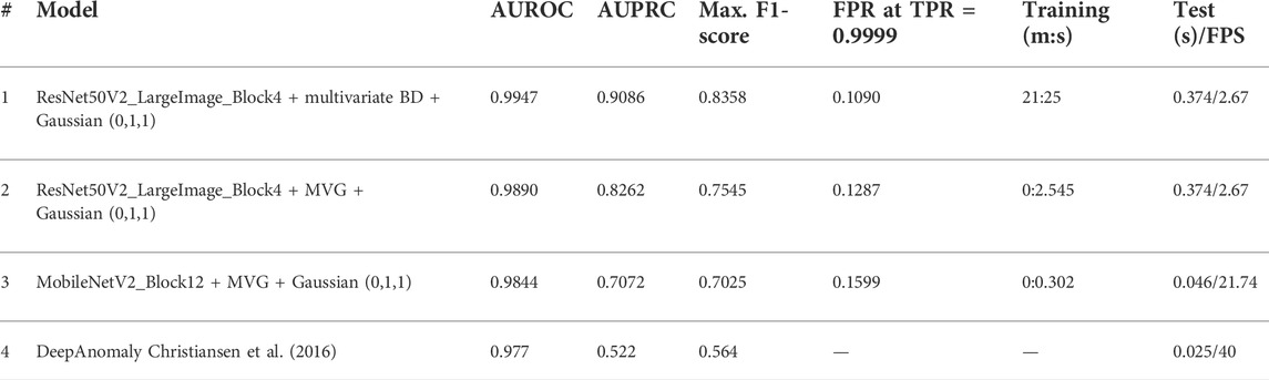
TABLE 3. Results for per-pixel classification and quantitative comparison to related work.

Model # 2 (ResNet50V2 cut at level 4 and blurred with a Gaussian in both spatial dimensions) has not only the smallest FPR but also exceeds in all other metrics using the full training data set.

Model # 3 relies on features from MobileNetV2 and achieves a very good FPR as well while being over 7 times faster. This results in about 22 frames per second (FPS), which is slightly faster than the frame rate of the camera, allowing the vehicle to process each frame before a new one is captured.

The best-performing model # 1 was trained by reducing the training data set from 20,025 to 2,314 patches with the balanced distribution approach. The resulting detector performs better for background objects, which were also present during training and should thus not be classified anomalous. A possible interpretation for this is that the normality distribution is skewed and the few patches of background objects are outnumbered by patches showing only the ground during training.

Model # 4 shows the work of Christiansen et al. as a comparison to the state of the art. They use a similarly specific custom data set and analogous methods. The maximum f1-score of 0.564 reported by them is significantly lower than the one achieved in this work (0.8358). This can be attributed to the more sophisticated neural network for feature extraction (ResNet vs. AlexNet) and the more powerful shallow classifier (multivariate balanced distribution vs. SVG) used in this work. The post-processing with a simple Gaussian blurring is also unique to this work and further improves the results (0.7583 without post-processing).

An inspection of the individual misclassifications in Figure 9 reveals that many of the still existing false negatives are actually due to imperfect labels or shadows. Per-pixel labels are not always ideal, which is the reason for most of the false negatives in the test data set. Some areas like shadows are hard to label because there is no clear objective for them. A shadow, while being a visual anomaly, does not represent an obstacle that needs to be avoided. Many publicly available data sets instead ignore the classification of shadows and do not count them as false positives or false negatives.

FIGURE 9

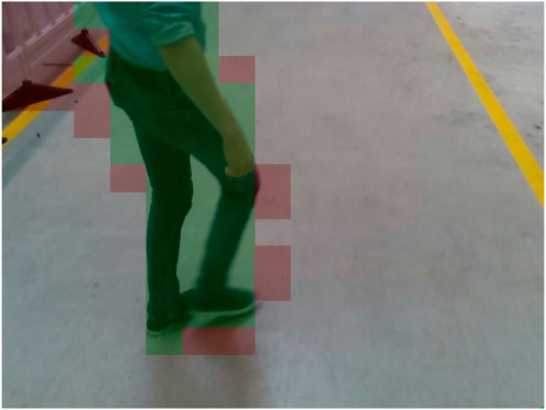
FIGURE 9. Correct detection of a human crossing the autonomous vehicles’ path with few false positives around the contour and in the background.

Figure 10 confirms that the multivariate Gaussian classifier outperforms the univariate Gaussian. The graphs show that both models can be improved by reducing the number of patches according to the balanced distribution.

FIGURE 10

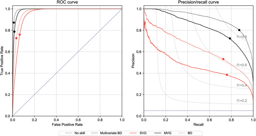
FIGURE 10. ROC (left) and PR (right) plots regarding the per-pixel metric of anomaly models using ResNet50V2 (large image, level 4) features and a Gaussian filter for postprocessing. The dot on the graph marks the threshold of maximum f1-score.

5.2 Per-frame metric

For the analysis of the anomaly detection in the per-frame metric model # three is chosen, since it already reaches perfect classification on the test data set. Perfect classification in this case means that each anomaly in a semicircle covering the lower half of the image is correctly detected and that there is no false alarm when there is no anomaly in the image at all. This is a promising result but it also raises some concerns and requires a more in-depth review.

In Figure 11 the model’s anomaly score is plotted over the successive frames of the test data set. Using a threshold of 17, the graph shows that all instances of humans as obstacles are detected with great confidence. Even small parts like an arm or shoes are detected. The fact that each frame is classified correctly draws interest to the images that are closest to the threshold. The peak at frame 80 for instance almost crosses the threshold, but actually contains no anomaly. This can be attributed to the fact that the automated vehicle took a slightly different path during training with the result that the barrier in the top left corner of frame 80 can only be seen partially. The same applies for the peaks around frame 40, 320, and 420, where the tool trolley on the side is more prominent than during training. More training data that better covers the complete operating environment could thus improve these edge cases and make selecting a robust threshold easier. As the MVG already achieves the highest possible scores for the per-frame metric, a multivariate balanced distribution is not considered. It should be noted that the multivariate balanced distribution does improve the per-pixel metric significantly and could also be used here to increase the margin where 100% classification accuracy is achieved. This could make choosing the right threshold a lot easier and increases the robustness of the classifier. The anomaly with the lowest score is the yellow line that was already discussed for the per-pixel metric.

FIGURE 11

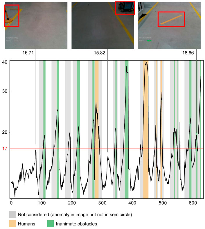
FIGURE 11. Per-frame anomaly scores (logarithmic scale) for the complete test sequence with a selection of interesting frames. Using a threshold of 17, each image is labeled correctly.

A possible point of critique could be the choice of the per-frame labels as introduced in section 3.4, because it discards many images with anomalies in them as “not considered”. These are also displayed in Figure 11 using a gray background. It can be observed that these images would at times be classified as anomalous, at other times as normal. This is actually the predicted behavior and it is compliant with the specific use case of obstacle detection, which has to focus first and foremost on safety. The classifier detects every instance of an obstacle close to the vehicle (using the semicircle criterion) and correctly classifies images with no obstacle as normal. The cases in between where an obstacle is at the top border, for example, are not relevant for the use case, because the vehicle can continue to drive until the obstacle is close. Stopping too early, on the other hand, is also allowed since this could only increase safety. If the obstacle cannot be seen anymore (a human leaves the view for example), the vehicle would continue driving. The only downside could be a slightly reduced availability because of unnecessary stops.

6 Comparison with classic approaches

To compare the anomaly detection’s performance with a semantic segmentation, the U-Net architecture by Ronneberger et al. (Ronneberger et al., 2015) is trained for obstacle detection. Since the amount of training data is not sufficient for a supervised learning from scratch, we add simulated data from a virtual factory environment, which was built in Unreal Engine four for this purpose. Thus, we generate 15.000 images. Data augmentation helps bridging the gap between real and simulated data.

This way the U-Net is able to segment all objects from the drivable path in the real world testing data. Applying the per-frame metric, the algorithm achieves a maximum f1-score of 0.85. This comparison shows that the anomaly detection is nearly as powerful as the semantic segmentation in the obstacle detection use case, although only 89 images instead of 15.000 images are used for training. While training the semantic segmentation requires ground truth segmentation labels for all the training data, the anomaly detection does not require any labeling. Looking at the practical application, generating training data by setting up a simulation environment or labeling images by hand generates high costs. The anomaly detection enables engineers to train the algorithm by using data from only one run.

7 Summary and future work

In this paper, we addressed the use case of vision-based obstacle detection for automated vehicles in industrial environments. Since supervised learning methods require huge amounts of labeled training data, we interpreted the task as a visual anomaly detection. On a specially recorded use case specific data set, the deep-hybrid approach shows good classification results. Due to the used pre-trained neural networks, we can limit the training phase to 89 images. Analysing the anomaly detection in a per-frame metric, we show that every human obstacle would be detected reliably even though some misclassifications occur in the per-pixel metric. For obstacle detection in a use case with limited complexity, the anomaly detection approach is on par with a semantic segmentation, which has been trained on 15.000 labeled images. The anomaly detection approach is therefore a low-cost alternative for obstacle detection. Using state-of-the-art neural networks for data processing, it offers a complex image understanding, which can be as robust as classic approaches, e.g. a semantic segmentation. The shallow classifier, however, limits the output complexity. As a consequence, the anomaly detection can only differentiate two classes and has a lower resolution of object boundaries.

In future work, the classification could be further improved if objects’ positions would be explicitly considered in the classification of image patches. Thus, a barrier in front of the vehicle would be different to one at the side of the path.To bring the algorithm into application, a verification of the requirements is needed. To address functional safety, it is necessary to assess the effects of environmental influences like illumination changes. Additional data from the field can be used to provide a statistical proof of safety.

Data availability statement

The original contributions presented in the study are included in the article/supplementary material, further inquiries can be directed to the corresponding author.

Author contributions

MW Conceptualization, Writing, Methodology, Software, Data Curation; TA Writing—Review; PB Funding Acquisition, Resources.

Funding

The development and testing of automated vehicle logistics is carried out within the framework of the AIMFREE research project (funding code: 01MV19002A). The project is funded by the German Federal Ministry of Economics and Energy (BMWi) in the guideline for a joint funding initiative to promote research and development in the field of electromobility and is supported by the project management agency Deutsches Zentrum für Luft-und Raumfahrt e.V. (DLR-PT).

Conflict of interest

The authors declare that the research was conducted in the absence of any commercial or financial relationships that could be construed as a potential conflict of interest.

Publisher’s note

All claims expressed in this article are solely those of the authors and do not necessarily represent those of their affiliated organizations, or those of the publisher, the editors and the reviewers. Any product that may be evaluated in this article, or claim that may be made by its manufacturer, is not guaranteed or endorsed by the publisher.

References

Almalioglu, Y., Saputra, M. R. U., Gusmão, P. P. B. d., Markham, A., and Trigoni, N. (2019). “Ganvo: Unsupervised deep monocular visual odom-etry and depth estimation with generative adversarial networks,” in International Conference on Robotics and Automation (ICRA), 5474–5480.

CrossRef Full Text | Google Scholar

Andrews, J., Morton, E., and Griffin, L. (2016). Detecting anomalous data using auto-encoders. Int. J. Mach. Learn. Comput. 6 (1), 21. doi:10.18178/ijmlc.2016.6.1.565

CrossRef Full Text | Google Scholar

Badrinarayanan, V., Kendall, A., and Cipolla, R. (2017). SegNet: A deep convolutional encoder-decoder architecture for image segmentation. IEEE Trans. Pattern Anal. Mach. Intell. 39 (12), 2481–2495. doi:10.1109/tpami.2016.2644615

PubMed Abstract | CrossRef Full Text | Google Scholar

Bergmann, P. (2018). Improving unsupervised defect segmentation by applying structural similarity to autoencoders, arXiv:1807.02011

Google Scholar

Bouindour, S., Snoussi, H., Hittawe, M. M., Tazi, N., and Wang, T. (2019). An on-line and adaptive method for detecting abnormal events in videos using spatio-temporal ConvNet. Appl. Sci. 9 (4), 757. doi:10.3390/app9040757

CrossRef Full Text | Google Scholar

Chandola, V., Banerjee, A., and Kumar, V. (2009). Anomaly detection: A survey. ACM Comput. Surv. 41 (3), 1–58. doi:10.1145/1541880.1541882

CrossRef Full Text | Google Scholar

Christiansen, P., Nielsen, L. N., Steen, K. A., Jørgensen, R. N., and Karstoft, H. (2016). DeepAnomaly: Combining background subtraction and deep learning for detecting obstacles and anomalies in an agricultural field. Sensors 16 (11). doi:10.3390/s16111904

PubMed Abstract | CrossRef Full Text | Google Scholar

Ergen, T., Mirza, A. H., and Kozat, S. S. (2017). Unsupervised and semi-super-vised anomaly detection with LSTM neural networks. arXiv:1710.09207

Google Scholar

European Commission (2019). Regulation of the European parliament and of the council. The European Parliamant, Brussels: European Union: PE-CONS 82/19.

Google Scholar

Feng, T., and Gu, D. (2019). Sganvo: Unsupervised deep visual odometry and depth estimation with stacked generative adversarial networks. IEEE Robot. Autom. Lett. 4 (4), 4431–4437. doi:10.1109/lra.2019.2925555

CrossRef Full Text | Google Scholar

Haselmann, M., Gruber, D. P., and Tabatabai, P. (2018). Anomaly detection using deep learning based image completion” in 17th IEEE International Conference on Machine Learning and Applications (ICMLA), 1237.

He, K., Zhang, X., Ren, S., and Sun, J. (2016a). “Deep residual learning for image recognition,” in IEEE Conference on Computer Vision and Pattern Recognition (CVPR), 770–778.

CrossRef Full Text | Google Scholar

He, K., Zhang, X., Ren, S., and Sun, J. (2016b). “Identity mappings in deep residual networks,” in European Conference on Computer Vision, 630–645.

CrossRef Full Text | Google Scholar

Howard, A. G., Zhu, M., Chen, B., Kalenichenko, D., Wang, W., Weyand, T., et al. (217). MobileNets: Efficient convolutional neural networks for mobile vision applications”, arXiv:1704.04861

Google Scholar

Klappstein, J. (2008). Optical-flow based detection of moving objects in traffic scenes, dissertation. Heidelberger Dokumentenserver. doi:10.11588/heidok.00008591

CrossRef Full Text | Google Scholar

Krizhevsky, A., Sutskever, I., and Hinton, G. E. (2012). ImageNet classification with deep convolutional neural networks. Adv. Neural Inf. Process. Syst. 60 (6), 1097–1105. doi:10.1145/3065386

CrossRef Full Text | Google Scholar

Lawson, W., Bekele, E., and Sullivan, K. (2017). “Finding anomalies with generative adversarial networks for a patrolbot,” in IEEE Conference on Computer Vision and Pattern Recognition Workshops (CVPRW), 12–13.

CrossRef Full Text | Google Scholar

Minematsu, T., Shimada, A., Uchiyama, H., Charvillat, V., and Taniguchi, R. i. (2018). Reconstruction-based change detection with image completion for a free-moving camera. Sensors 18 (4), 1232. doi:10.3390/s18041232

PubMed Abstract | CrossRef Full Text | Google Scholar

Mukojima, H. (2016). “Moving camera background-subtraction for obstacle detection on railway tracks,” in IEEE International Conference on Image Processing (ICIP), 3967.

CrossRef Full Text | Google Scholar

Rippel, O., Mertens, P., and Merhof, D. (2020). Modeling the distribution of normal data in pre-trained deep features for anomaly detection. arXiv:2005.14140

Google Scholar

Ronneberger, O., Fischer, P., and Brox, T. (2015). U-Net, : Convolutional networks for biomedical image segmentation. arXiv:1505.04597

Google Scholar

Russakovsky, O., Deng, J., Su, H., Krause, J., Satheesh, S., Ma, S., et al. (2015). ImageNet large scale visual recognition challenge. Int. J. Comput. Vis. 115 (3), 211–252. doi:10.1007/s11263-015-0816-y

CrossRef Full Text | Google Scholar

Sabokrou, M., Khalooei, M., Fathy, M., and Adeli, E. (2018). “Adversarially learned one-class classifier for novelty detection,” in IEEE Conference on Computer Vision and Pattern Recognition (CVPR), 3379–3388.

CrossRef Full Text | Google Scholar

Sandler, M., Howard, A., Zhu, M., Zhmoginov, A., and Chen, L.-C. (2018). “MobileNetV2: Inverted residuals and linear bottlenecks,” in IEEE Conference on Computer Vision and Pattern Recognition (CVPR), 4510–4520.

CrossRef Full Text | Google Scholar

Sarafijanovic-Djukic, N., and Davis, J. (2019). Fast distance-based anomaly detection in images using an inception-like autoencoder. Switzerland: Springer, 493–508.

CrossRef Full Text | Google Scholar

Schmidt, A. (2020). Kate — götting KG. [Online]. Available at: https://www.goetting-agv.com/kate (accessed Jun, 17, 2020).

Google Scholar

Simonyan, K., and Zisserman, A. (2014). Very deep convolutional networks for large-scale image recognition. arXiv:1409.1556

Google Scholar

Tan, M., and Le, Q. V. (2019). “EfficientNet: Rethinking model scaling for convolutional neural networks,” in International Conference on Machine Learning (ICML). arXiv:1905.11946.

Google Scholar

Wenning, M., Kawollek, S., and Kampker, A. (2020). Automated driving for car manufacturers’ vehicle logistics. A. T. - Autom. 68 (3), 222–227. doi:10.1515/auto-2019-0087

CrossRef Full Text | Google Scholar