Objectification of intracochlear electrocochleography using machine learning

Introduction: Electrocochleography (ECochG) measures inner ear potentials in response to acoustic stimulation. In patients with cochlear implant (CI), the technique is increasingly used to monitor residual inner ear function. So far, when analyzing ECochG potentials, the visual assessment has been the gold standard. However, visual assessment requires a high level of experience to interpret the signals. Furthermore, expert-dependent assessment leads to inconsistency and a lack of reproducibility. The aim of this study was to automate and objectify the analysis of cochlear microphonic (CM) signals in ECochG recordings.

Methods: Prospective cohort study including 41 implanted ears with residual hearing. We measured ECochG potentials at four different electrodes and only at stable electrode positions (after full insertion or postoperatively). When stimulating acoustically, depending on the individual residual hearing, we used three different intensity levels of pure tones (i.e., supra-, near-, and sub-threshold stimulation; 250–2,000 Hz). Our aim was to obtain ECochG potentials with differing SNRs. To objectify the detection of CM signals, we compared three different methods: correlation analysis, Hotelling's T² test, and deep learning. We benchmarked these methods against the visual analysis of three ECochG experts.

Results: For the visual analysis of ECochG recordings, the Fleiss' kappa value demonstrated a substantial to almost perfect agreement among the three examiners. We used the labels as ground truth to train our objectification methods. Thereby, the deep learning algorithm performed best (area under curve = 0.97, accuracy = 0.92), closely followed by Hotelling's T² test. The correlation method slightly underperformed due to its susceptibility to noise interference.

Conclusions: Objectification of ECochG signals is possible with the presented methods. Deep learning and Hotelling's T² methods achieved excellent discrimination performance. Objective automatic analysis of CM signals enables standardized, fast, accurate, and examiner-independent evaluation of ECochG measurements.

1. Introduction

Electrocochleography (ECochG) measures electrical potentials generated by the inner ear in response to acoustic stimulation. In patients with cochlear implant (CI), using the implanted electrode, these potentials can be picked up directly from the inner ear. The technique is increasingly used to monitor the inner ear function during and after implantation. Research groups were able to correlate changes in the ECochG signal with traumatic events during implantation (1–6).

In order to assess ECochG potentials (either intra or postoperatively), the analysis is most commonly performed by visual inspection, which is currently the gold standard. Therefore, the interpretation is heavily relying on the expertise of the examiner. This entails several problems: i) a high level of experience is needed to interpret the signals correctly. Thus, inexperienced clinicians and researchers are unable to exploit the technique; ii) the examiner determines whether or not an ECochG response is present, which may result in a lack of reproducibility; iii) longitudinal comparisons are hampered as the assessment is not absolutely identical. iv) research groups use different types of analysis, which makes the comparability of clinical findings and study results difficult or impossible (4, 7–12); v) due to the inconsistent assessment, patients with a poor signal-to-noise ratio (SNR) are often not reported. However, in order to draw correct conclusions, all measurements should be reported (13, 14); and vi) the analysis of ECochG signals is complex, which makes immediate judgment difficult. This is, of course, a prerequisite when an instant assessment is required (e.g., in the operating theater).

ECochG itself is an umbrella term for different electrophysiological signal components of the inner ear (i.e., the cochlear microphonic, CM, the auditory neurophonic, ANN, the compound action potential, CAP, the summating potential, SP). These signal components can be highlighted by measurements with different acoustic polarities (condensation, CON and rarefaction, RAR). The difference potential (DIF) is calculated by subtracting the CON and RAR polarities. The DIF response mainly represents the CM signal (15). In addition, the sum highlights the summating potential (SUM), which mainly represents the ANN (16). However, CM and ANN potentials cannot be isolated, especially at high stimulation levels and low frequencies (17). In intra and postoperative recordings, most commonly the CM/DIF signal is used as it is the largest and most robust signal component (18). For this reason, in this article, we will limit the analysis to the CM/DIF signal. Even though the CM/DIF signal is the strongest potential, there are some things to keep in mind. The amplitude of the signal is in the microvolt range and varies greatly between individuals. While certain patients show large amplitudes, in others, the potentials are very small, resulting in a poor SNR. Furthermore, the morphology and latency of the CM/DIF signal might vary significantly depending on the remaining intact hair cells (19–21). These factors (i.e., poor SNR, different wave morphology) must be taken into account when analyzing ECochG potentials.

For the reasons given above, an automated and objective evaluation would be highly desirable. This would standardize and significantly simplify the analysis of the signals and make it independent of the examiner. For ECochG signals, an approach using Fast Fourier Transform (FFT) has been proposed (18, 22–24). However, this method is not always applicable, especially for short signals, since they do not have a stationary period and adjacent frequencies cannot be accurately distinguished. For other electrophysiological signals, objectified analyses have become established in clinical practice. For example, for auditory brainstem responses (ABR), correlation analysis is used (25, 26). In the evaluation of cortical auditory evoked potentials (CAEP), Hotelling's T² test has yielded a sensitivity at least comparable to that of visual inspection (27–29). In other medical disciplines (i.e., identification of cardiac arrhythmias in electrocardiograms, ECGs), deep learning (DL) strategies could be successfully implemented (30–33).

The aim of this study was to automate and objectify the analysis of CM/DIF signals in ECochG recordings. The employed method should i) be comparable to visual analysis, (ii) allow the interpretation of intra- and postoperative ECochG signals by clinicians and researchers who do not have much experience in the field, (iii) allow immediate feedback, (iv) should be replicable by other clinical and research centers, (v) allow reproducible comparison of longitudinal data (since the same analysis is performed).

2. Materials and methods

This prospective cohort study was conducted in accordance with the Declaration of Helsinki and was approved by the local institutional review board (KEK-BE 2016-00887 and 2019-01578). All participants gave written informed consent before participation.

2.1. ECochG data

We performed ECochG measurements in 36 subjects (n = 41 ears). All subjects used a Med-El implant (MED-EL, Austria). Pure tone audiograms were performed in a certified acoustic chamber with a clinical audiometer (Interacoustics, Denmark). Hearing thresholds were collected either immediately preoperatively or, in the case of postoperative measurements, on the same day as the ECochG measurement. We obtained pure tone air conduction hearing thresholds in dB hearing level (HL) at 125, 250, 500, 750, 1,000, 1,500, 2,000, and 4,000 Hz using either headphones or plug-in earphones. Pure tone averages (PTAs) were calculated as the mean hearing threshold at 125, 250, 500, and 1,000 Hz. PTAs and patient demographics are shown in Table 1.

TABLE 1

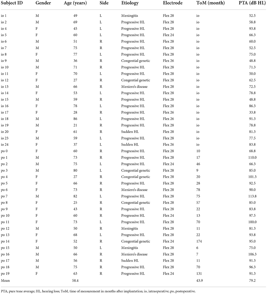
Table 1. Demographic of included subjects.

We recorded ECochG potentials using the Maestro Software (version 8.03 AS and 9.03 AS, MED-EL, Austria). The system setup was identical to our previous study (10). We measured ECochG potentials at electrodes 1, 4, 7, and 10 (with electrode 1 at the tip) and only at a stable electrode position (i.e., either intraoperatively after completed electrode insertion or in a postoperative setting). When stimulating, depending on the individual hearing threshold, we used three different intensity levels: supra-threshold level (5 dB below discomfort level), near-threshold level (10 dB above hearing threshold), and sub-threshold level (10 dB below hearing threshold). Thereby, the acoustic amplitude level was restricted as shown in Table 2. Our aim was that not all stimulations would elicit an ECochG response and that, depending on the stimulation level, the SNR was different. As an acoustic stimulus, we used pure tones with settings shown in Table 2. ECochG potentials were recorded with two polarities (i.e., CON, and RAR). For each ECochG response, we recorded 100 epochs per polarity. The two polarities were subtracted to form the CM/DIF signal.

TABLE 2

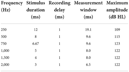
Table 2. Settings for acoustic stimulation and maximum possible acoustic stimulation level (maximum amplitude).

2.2. Preprocessing of ECochG signals

As preprocessing, we used the following steps: i) if present, removal of stitching artifacts, ii) application of a Gaussian weighted averaging method to increase the SNR and exclude uncorrelated epochs from further analysis, and iii) a 2nd order, forward-backward filtered Butterworth bandpass filter (cutoff frequencies 10 Hz / 5 kHz for visual analysis, and 100 Hz / 5 kHz for objective evaluation methods). To increase the SNR in our ECochG recordings, we calculated the Gaussian weighted epochs S_GE(i) as described by Davila et al. (34) and Kumaragamage et al. (35). We used the following equation:

$\begin{array}{l}{S}_{GE(i)}={\displaystyle \sum _{l=-2}^2}(e^{-\left[0.5{(\frac{l}{\sigma ·(5-1)/2})}^2\right]}·S_{E(i+l)})\end{array}$

whereas, l is the index number, starting from –2 to 2 that accounts for five epochs S_E averaged under the Gaussian window, and i is the index number of the epochs in S_E. The SD of the Gaussian window σ was set to 0.4. Each Gaussian weighted epoch S_GE(i) was then correlated with the mean of all epochs S_approx. S_GE(i) with a correlation less than –0.2 were excluded to form the final ECochG response S. If more than 10% of epochs had to be removed, only the 10 worst correlated were discarded. Finally, we calculated the SNR using the +/- averaging method (36).

2.3. Visual analysis

ECochG data were visually analyzed by three examiners with extensive experience in the field. The goal was to have a labeled data set that was used i) to train and test the objective algorithms, and ii) to obtain a benchmark for evaluating the accuracy, specificity, and sensitivity of the objective detection methods. Using Labelbox (37), the data were presented to the examiners as a subplot with six individual graphs representing i) the DIF response, ii) the SUM response, iii) the CON and RAR responses, and iv-vi) their individual FFT traces (an example is shown in the Supplementary material). Each examiner had to assess 4133 ECochGs with the question if a CM/DIF response was present or not (dichotomous question). Thereby, we used a blinded design in which the investigators did not discuss the assessment to avoid bias in the individual assessment. Signals classified as CM/DIF response by two examiners (and noise by one examiner) were presented a second time to all three examiners (to minimize volatility errors). Only ECochG signals that were finally considered valid responses by all three investigators were classified as responses. These were used as ground truth for the objective classification. We used Fleiss' kappa to compare the raters. Fleiss' kappa is a measure of agreement between multiple raters in classifying items (38).

2.4. Objective detection methods

We included the following objective detection methods: i) Hotelling's T² test, ii) correlation analysis, and iii) a DL convolutional neural network (CNN). To train and evaluate our objective analysis, we benchmarked these methods against the visual analysis of the three experts.

The dataset was divided into two parts: 70% for training and 30% for testing purposes. We used the training subset to train and validate the models. For training, both features (ECochG signals) and labels (ground truth determined by the examiners) were provided. The test set was used to evaluate the performance of the model. Here, only features were provided. The predictions of the model were then compared to the labels.

2.4.1. Hotelling's T² test

Based on Hotelling's T² method described by Golding et al. and Chesnaye et al. for objective detection of CAEP signals, we adapted the method to ECochG signals (27, 29). The Hotelling's T² test for one sample is a multivariate extension of the Student's t-test (39, 40). With Hotelling's T² test, we can test the null hypothesis (H0) whether Q features are statistically different from Q hypothesized values.

In our case, the ECochG recordings were the features and the hypothesized values were noise. The ECochG recordings were divided into Q windows along the time axis called 'time-voltage-means' (TVMs). The mean value was taken from each Q-window, resulting in the following N × Q voltage matrix V:

$\begin{array}{l}V=\left[\begin{array}{ccc}{v}_{11}& \dots & v_{1Q}\\ ⋮& \ddots & ⋮\\ v_{N1}& \dots & v_{NQ}\\ \end{array}\right]\end{array}$

Where N was the number of epochs and v_ij the j^th voltage means from the i^th epoch. The corresponding hypothetical values (noise) were an array of size 1 × Q filled with zeros. The noise was zero because the expected mean value of an ECochG signal should be zero due to the bandpass filtering. The number of used TVMs resulted in a down sampling, illustrated in Figure 1.

FIGURE 1

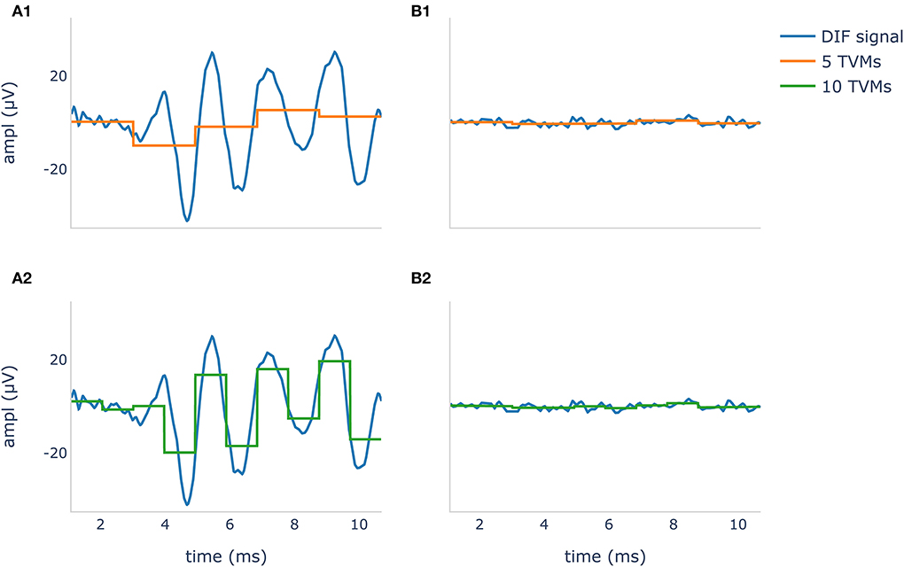
Figure 1. Difference potential (DIF) curves in blue show a recognizable CM/DIF signal (A1,A2) and noise with no visible CM/DIF component (B1, B2) in response to a 500 Hz stimulus. The orange curve in (A1,B1) shows 5 time-voltage-means (TVMs), and the green curve in (A2,B2) shows 10 TVMs used to calculate Hotelling's T² test. It is evident that in this example, an increase of the TMVs leads to better mapping of the CM/DIF signal with higher accuracy.

We performed the calculations using a python (v 3.9.7) script and the hotellings function from the spm1d module (v 0.4) (41, 42). As significance level α, we used 0.01 to tune the number of voltage means Q for each acoustic stimulus frequency individually. The optimal number of TVMs for the Hotelling T² test was calculated based on the maximum accuracy. For this purpose, the number of TVMs was successively increased in steps of five from 5 to 195 and the Hotelling's T² test was calculated on the training set.

2.4.2. Correlation analysis

Our correlation algorithm is based on the method of Wang et al. which explores the correlation of ABR signals (26). The correlation procedure relies on the repeatability of the similarity of two waveforms. The degree of similarity can be quantified by calculating the Pearson correlation coefficient. A positive correlation close to one reflects the presence of a response, while a zero correlation shows the absence of response (25).

In our calculations, we treated the two polarities (CON/RAR) separately and finally averaged the correlation coefficients. The two polarities were separate, treated as they evolve inversely (which is caused by condensation and rarefaction phased acoustic stimuli). The procedure is shown in Figure 2. Finally, we fitted a logistic regression model based on the correlation coefficients.

FIGURE 2

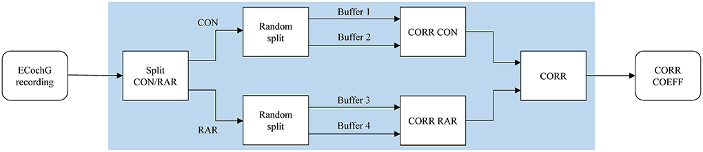
Figure 2. The correlation analysis handles CON and RAR recordings separately and proceeds as follows: (i) the ECochG recordings are divided into CON and RAR; (ii) CON and RAR are each divided into two randomly arranged buffers of the same size (Buffers 1–4, 50 epochs each); (iii) the Pearson correlation coefficients for CORR CON and CORR RAR are calculated from buffer 1 and 2 and buffer 3 and 4, respectively; (iv) CORR is calculated from the mean of CORR CON and CORR RAR. Since CORR depends on the subdivision of buffers, steps ii–iv (shaded area) are repeated 100 times and averaged to get the final correlation coefficient CORR COEFF. CON, condensation; RAR, rarefaction; CORR, correlation; COEFF, coefficient.

2.4.3. Deep learning

Our DL classification approach was based on the method used to automatically identify cardiac arrhythmia in ECG signals. Several DL approaches to cardiac arrhythmia detection have been proposed in the literature (30–33). Among them, time frequency scalograms using continuous wavelet transform (CWT) and AlexNet showed convincing results (32, 33). AlexNet is a large convolutional neural network (CNN) containing about 6,50,000 neurons and 60 million parameters. It consists of five convolutional layers, and three fully connected layers and is optimized for image classification (43).

Time frequency scalogram images for the classifier were generated from our dataset using CWT and the Python module PyWavelets (44). In this process, a Morlet wavelet shrinks and expands to map the signals into a time-frequency scalogram. We chose the Morlet wavelet because it offers a good compromise between spatial and frequency resolution (33, 45). We normalized the scalograms and compressed them to a dimension of 224 × 224 × 3 for width, height, and depth (red, green, blue). ECochG DIF traces and their wavelet transformation are shown in Figure 3.

FIGURE 3

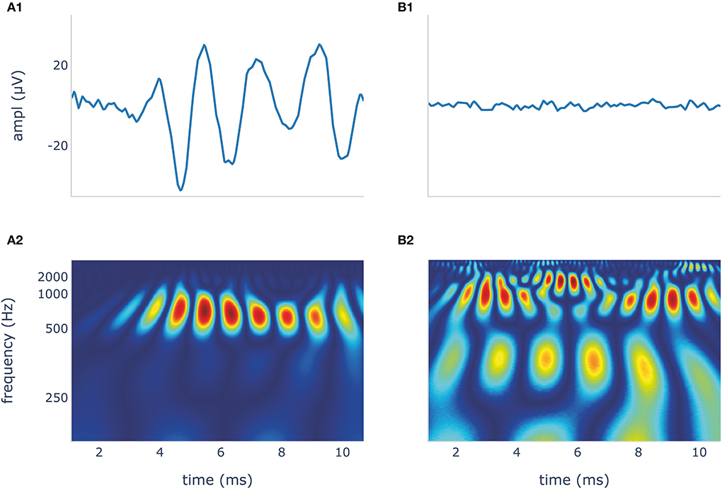
Figure 3. The blue DIF curves (A1,B1) show a recognizable CM/DIF signal (A1) and noise with no visible CM/DIF component (B1), respectively, in response to a 500 Hz stimulus. Their corresponding time frequency scalograms generated using continuous wavelet transformation (CWT) are shown in (A2,B2). These scalograms were then used to train and test the deep learning algorithm. DIF, difference; CM, cochlear microphonic.

We used PyTorch (v 1.11.0) and the pre-trained (on the ImageNet database) AlexNet loaded from torchvision (v 0.6.0) to take advantage of the already good classification properties (46, 47). We substituted the last two classifiers of the AlexNet for binary classification output. The rest of the network was left exactly as it was during initialization. Stochastic gradient descent with momentum was used to train the model. The mini-batch size was 8 and the maximum epoch was 25 with the learning rate being 1e-4, and a momentum of 0.9. We used 10-fold cross-validation to detect overfitting. We then trained the model with the full training set to increase model performance.

2.5. Statistical analysis

We used accuracy, sensitivity, and specificity to evaluate our algorithms. The algorithms were compared using the area under the receiver operating characteristic (ROC) curve, also known as the area under the curve (AUC). We used a one-sided DeLong test with a confidence level of 0.95 using the roc.test function of the pROC package (v 1.18.0) with R (v 4.1.2) (48, 49).

3. Results

3.1. ECochG recordings and preprocessing

Gaussian weighted averaging significantly increased the mean SNR from 2.50 dB (standard deviation, SD, 2.39) to 4.18 dB (SD 1.86) as demonstrated by the one-tailed paired-samples t-test (p < 0.001). In total, 4133 DIF signals were labeled visually by the three experts. Labeling took between 13.5 and 15 h (on average, 12 s per signal). In contrast, objective analysis using the algorithms took less than 25 ms per signal (the duration was determined on a notebook XPS 13 9360 (Dell, Round Rock, TX, USA) and does not include the training time of the algorithms, which was substantially longer).

3.2. Visual analysis

The Fleiss' kappa value of the agreement for the examiners and all stimulation frequencies are shown in Table 3. Results demonstrated a substantial to almost perfect agreement among the examiners (50). Particularly, for the mid-frequencies (500 Hz – 1 kHz), the examiners were very much in agreement. This agreement was a little lower for the lowest (i.e., 250 Hz) and the two highest frequencies (i.e., 1,500 and 2,000 Hz), but still substantial. However, between the three examiners, there was a systematic discrepancy in the visual assessment. The false-positive rates (FPRs) for examiners 1, 2, and 3 were 0.110, 0.068, and 0.032, respectively. That is examiner 1 still considered signals with a lot of noise as valid responses, whereas examiner 3 only accepted clearer neurophysiological traces.

TABLE 3

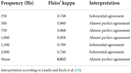
Table 3. Fleiss' kappa among all three examiners.

Table 4 shows an overview of the stimulation frequencies, the stimulation levels, the SNR, and the number of signals where the experts identified a CM/DIF response. For frequencies of 500 Hz and above, when stimulated at supra-threshold level, a clear CM/DIF component was found in 53.3%.

TABLE 4

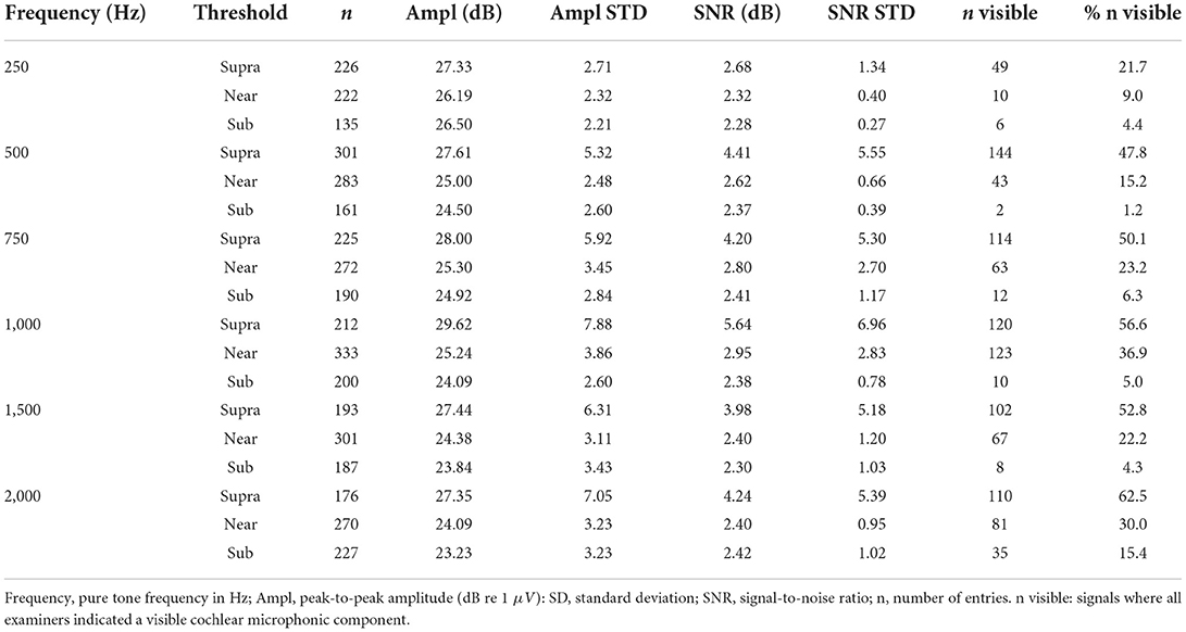
Table 4. Overview of the stimulation frequencies, the individual intensities, and the SNR.

For all frequencies, the supra-threshold stimulation showed the largest amplitudes (p < 0.001, one-tailed paired-samples t-test), the biggest SNR (p < 0.001) as well as the most visible signals. Near-threshold stimulation showed larger amplitudes (p < 0.001), and bigger SNR (p < 0.001) than sub-threshold stimulation. However, this was not the case for 250 Hz stimulation amplitudes (p = 0.104). Regarding visual analysis, near-threshold levels showed significantly more visible CM/DIF responses than sub-threshold levels, except at 250 Hz. At this frequency, we identified the same number of responses for near-threshold and sub-threshold levels.

3.3. Comparison of objectification methods

All objectification methods presented in Table 5 showed good performance in detecting CM/DIF responses (51). The ROC curves of the objectification methods for all mixed frequencies are shown in Figure 4. The DL method performed best (AUC = 0.97, accuracy = 92%), followed closely by Hotelling's T² test (AUC = 0.96, accuracy = 91%). Statistically, this difference was not significant (p = 0.14). In contrast, the correlation analysis method underperformed as a classifier (AUC = 0.85; accuracy = 83%). This difference was statistically significant (DL p < 0.001; Hotelling's T² test p < 0.001). Table 5 shows the performance of the algorithms for all frequencies.

TABLE 5

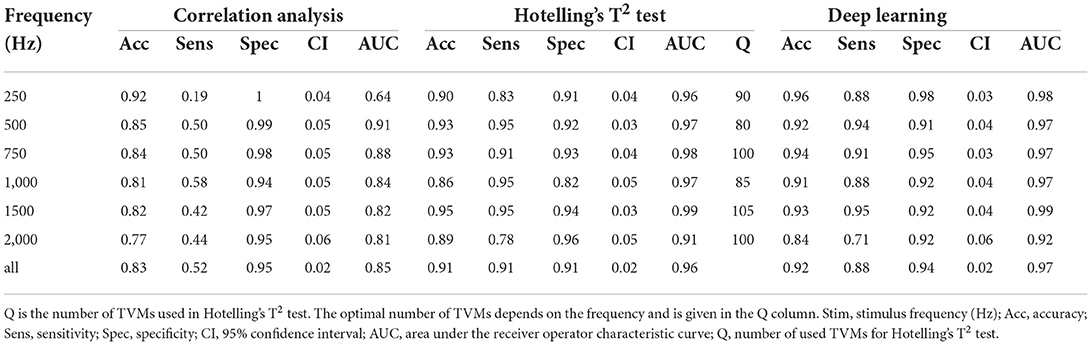
Table 5. Performance of objectification methods.

FIGURE 4

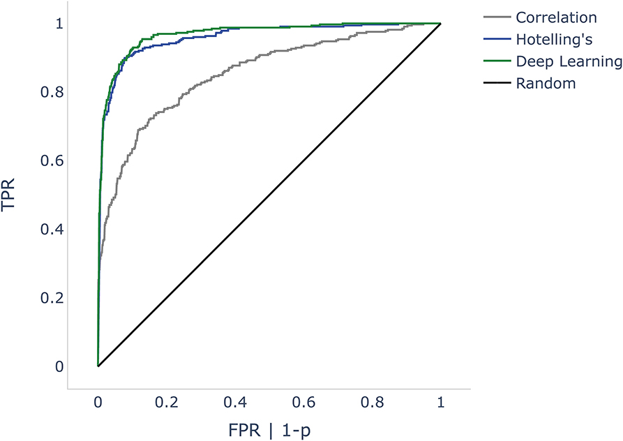
Figure 4. ROC curves comparing correlation analysis, Hotelling's T² test, and deep learning (DL) methods. The false positive rate (FPR) is the dependent variable (x-axis) in the DL and correlation algorithms. As Hotelling's T² test does not specify probabilities, we used p-values instead. Since p is inversely proportional to probabilities, we mapped 1-p. The black line shows a random classifier. ROC, receiver operator characteristic; p, p-value.

4. Discussion

This study demonstrates that it is possible to objectively and automatically determine whether a CM/DIF response is present or not. All three algorithms investigated showed very good to excellent discrimination performance. Especially Hotelling's T² test and the DL method revealed excellent results (mean accuracy was 91 and 92% with an AUC of 0.96 and 0.97, respectively).

4.1. Preprocessing

ECochG traces are usually displayed as averaged signals (both, intra,- and postoperatively). During signal recordings, noisy epochs can affect the signal quality and reduce SNR (34). In addition, there are large inter-individual differences. While some patients show very prominent potentials, in others the signal amplitude is small (1, 3, 10, 12, 52). If ECochG is to be used routinely in the operating room and postoperative setting, however, all patients (including those with small signals) must be analyzed. In our cohort, the previously described Gaussian weighted averaging method (34, 35) showed a substantial increase in SNR of ECochG signals of all frequencies. Our calculations improved the mean SNR by 1.68 dB. Kumarange et al. were able to improve the SNR by 3.5 dB. However, they used extracochlear ECochG recordings, whereas we measured from inside the cochlea.

4.2. Visual analysis

In our study, the visual evaluation of the data was carried out by three independent examiners who have many years of experience in this field. Per recording, it took them 12 s on average to judge if a signal was present or not. In contrast, with the described computer algorithms, the evaluation was available after a few milliseconds. This time span may not sound like much. But it is crucial, especially in the intraoperative real-time setting, where immediate decisions must be made to prevent possible inner ear injury.

Regarding the visual analysis, the agreement of the three examiners was very good, especially in the frequency range between 500 and 1,000 Hz. Disagreements occurred mainly in borderline cases with low SNRs (another reason why the SNR needs to be improved, if possible). The agreement among the experts was still substantial, but lower 250 Hz and for the two highest frequencies (i.e., 1,500 and 2,000 Hz). At 250 Hz, among all measured intracochlear ECochG, the SNR was the lowest (also refer to Table 4) (8). For the two highest frequencies, in some cases, it was difficult to distinguish between natural signal fluctuations and reproducible CM/DIF signal components.

It is important to note that a low SNR can affect the waveform morphology. In our data, e.g., CON and RAR responses did not evolve in opposite directions to each other, or there was a change in the usual morphology (e.g., the characteristic frequency of the CM/DIF signal was too low, or the ECochG traces had an irregular shape). This resulted in one examiner detecting a CM/DIF response while the other detected only noise. In our analysis, we found that the overall agreement was high, but one expert was rather cautious and another more tolerant in his assessment. This issue can be addressed by using an automated, quantitative and objective evaluation method, as suggested by our study. This allows for a uniform evaluation of the signals, which simplifies the comparison between individuals and different implantation centers or even makes it possible in the first place.

The analysis of the three stimulation levels showed that supra-threshold stimulation most frequently elicited a visually present CM/DIF signal. In addition, the SNR (except at 250 Hz) was substantially higher compared to the near- and sub-threshold levels. With supra-threshold stimulation, in our cohort, for the frequencies 500 Hz and above, a clear CM/DIF response was detected in 53.3% of cases. This implies that in a significant proportion of cases, no clear response could be detected. Additionally, this is despite the fact that most of the measurements took place in a postoperative setting and patients had a measurable residual hearing on the day of examination. However, it should be noted that the PTA of our study population shows a large variance and was, in some individuals, above 90 dB (compare Table 1). Consequently, the stimulus intensity was not always equally above the hearing threshold. In addition, recordings were measured from 4 different electrodes. For many subjects, ECochG responses were not visible at all electrodes. In literature, the situation regarding the prevalence of CM/DIF responses when stimulating above the hearing threshold is controversial. While some authors have found a close correlation between hearing threshold and CM/DIF signal threshold (11), other scientists have not found a clear relationship (1, 2, 8, 9, 12, 22, 23). Based on our data (refer to Table 4), we must assume that this correlation is both level- and frequency-dependent. For near-threshold and sub-threshold simulations, we detected significantly fewer visually detectable ECochG signals. Interestingly, the sub-threshold stimulation also showed CM/DIF responses in some cases (9, 23). Especially at 2,000 Hz, this finding was more pronounced.

4.3. Comparison of the objectification methods

In our study, DL with CNN AlexNet on time-frequency scalogram plots using CWT showed the best discrimination performance. The advantage of this method is that the morphology of the electrophysiological signal is taken into account. Similar to visual inspection, our algorithm was able to identify the CM/DIF response in the time-frequency scalograms shown in Figure 3. Another advantage of DL is its independence from preprocessing steps of ECochG signals (e.g., filtering). We trained our network with both, filtered and unfiltered data and could observe an almost identical accuracy of 90%.

Hotelling's T² test showed the highest sensitivity of our tested algorithms. This high sensitivity is also known from other research (27–29). However, in order to achieve good results with the Hotelling T² method, the signal must be free of artifacts and baseline wander. Both signal phenomena occur in ECochG measurements and must be addressed by using preprocessing steps. Furthermore, an optimal length of the TVMs must be defined. This is a trade-off; if the TVMs are too long, they contain the natural fluctuation of the ECochG signal (e.g., peaks and valleys). This results in TVMs with zero amplitude (similar to noise). If the TVMs are too short, the robustness and thus the test sensitivity decreases (overfitting) (29, 39).

Finally, the correlation analysis gave good objectivity to our data, although it did not reach the performance of the other two methods. It should be noted that signal artifacts can also have a high correlation and thus reduce the accuracy of this method. Such artifacts arise, e.g., from stitching or other unwanted effects (25). To overcome this, one could try to eliminate artifacts with more elaborate techniques or correlate only segments that are not affected.

In summary, the DL algorithm and Hotelling's T² test are very well suited for the objective assessment of ECochG signals; we achieved a high accuracy with both approaches. By using one of these methods, we can evaluate CM/DIF signals independently of the expertise of the examiner. In this article, we focused on the methodology itself with the question of whether a CM/DIF response was present or not. In the next step, further calculations could be included. For example, the evolution of amplitude or latency during electrode insertion. Furthermore, the advantages of the methodology are the immediate result as well as the reproducibility, which allows the comparison i) between individuals, ii) between different implant centers as well as iii) of longitudinal data. Finally, an automated ECochG assessment tool would pave the way for future standardized and widespread use in the clinical setting.

4.4. Limitations

Our data set was limited to 4133 ECochG recordings. Additional signals would further improve the methodology, increase the generalization of our models and reduce overfitting. Moreover, the data were visually reviewed by three experts. If more experts were incorporated into the algorithm, this may also refine the evaluation. Systemic noise can hamper the use of objective algorithms. In particular, the correlation analysis and Hotelling's T² test were found to be vulnerable. The DL method on the other hand was less dependent on data preprocessing and less sensitive to noise interference.

We have applied our methodology only when the electrode position was stable. In the next step, the objectification methods must also be tested during insertion, i.e., when the electrode is in motion. Furthermore, in the current study, we restricted ourselves to the CM/DIF signal. However, the methodology could also be used for the other signal components (i.e., ANN/SUM, CAP, SP). The combination of different data features is also advisable (4, 53) and must be evaluated in a future study.

5. Conclusion

Objectification of ECochG signals is possible with the methods presented in this paper. Our DL algorithm and Hotelling's T² test achieved a high accuracy to detect CM/DIF responses that had previously been identified by three ECochG experts. Objective automatic analysis of CM/DIF signals enables standardized, fast, accurate, and examiner-independent evaluation of ECochG measurements.

Data availability statement

The raw data supporting the conclusions of this article will be provided by the authors upon request.

Ethics statement

The studies involving human participants were reviewed and approved by the Cantonal Ethics Committee of Bern (BASEC ID 2019-01578). Written informed consent to participate in this study was provided by the participants' legal guardian/next of kin.

Author contributions

KS performed the measurement, wrote the software and article, and labeled and analyzed the data. WW analyzed the data and provided interpretive analysis and critical revision. AD labeled the data. CR, MC, and GM provided interpretive analysis and critical revision. SW designed the experiment, analyzed the data, labeled the data, and provided interpretive analysis and critical revision. All authors contributed to the article and approved the submitted version.

Funding

This study was partly funded by the Department of Otorhinolaryngology, Head and Neck Surgery at the Inselspital Bern, the Clinical trials unit (CTU) research grant, and the MED-EL company. GM was supported by the Swiss National Science Foundation #320030_173081. The authors declare that this study received funding from MED-EL Germany. The funder was not involved in the study design, collection, analysis, interpretation of data, the writing of this article or the decision to submit it for publication.

Acknowledgments

The authors would like to thank Marek Polak and his team from MED-EL, Austria, for their support.

Conflict of interest

The authors declare that the research was conducted in the absence of any commercial or financial relationships that could be construed as a potential conflict of interest.

Publisher's note

All claims expressed in this article are solely those of the authors and do not necessarily represent those of their affiliated organizations, or those of the publisher, the editors and the reviewers. Any product that may be evaluated in this article, or claim that may be made by its manufacturer, is not guaranteed or endorsed by the publisher.

Supplementary material

The Supplementary Material for this article can be found online at: https://www.frontiersin.org/articles/10.3389/fneur.2022.943816/full#supplementary-material

References

1. Campbell L, Kaicer A, Sly D, Iseli C, Wei B, Briggs R, et al. Intraoperative real-Time cochlear response telemetry predicts hearing preservation in cochlear implantation. Otol Neurotol. (2016) 37:332–8. doi: 10.1097/MAO.0000000000000972

PubMed Abstract | CrossRef Full Text | Google Scholar

2. Dalbert A, Pfiffner F, Hoesli M, Koka K, Veraguth D, Roosli C, et al. Assessment of cochlear function during cochlear implantation by extra- and intracochlear electrocochleography. Front Neurosci. (2018) 12:18. doi: 10.3389/fnins.2018.00018

PubMed Abstract | CrossRef Full Text | Google Scholar

3. Weder S, Bester C, Collins A, Shaul C, Briggs RJ, O'Leary S. Toward a better understanding of electrocochleography: analysis of real-time recordings. Ear Hear. (2020) 41:1560–7. doi: 10.1097/AUD.0000000000000871

PubMed Abstract | CrossRef Full Text | Google Scholar

4. Weder S, Bester C, Collins A, Shaul C, Briggs RJ, O'Leary S. Real Time monitoring during cochlear implantation: increasing the accuracy of predicting residual hearing outcomes. Otol Neurotol. (2021) 42:E1030–6. doi: 10.1097/MAO.0000000000003177

PubMed Abstract | CrossRef Full Text | Google Scholar

5. Bester C, Weder S, Collins A, Dragovic A, Brody K, Hampson A, et al. Cochlear microphonic latency predicts outer hair cell function in animal models and clinical populations. Hear Res. (2020) 398:108094. doi: 10.1016/j.heares.2020.108094

PubMed Abstract | CrossRef Full Text | Google Scholar

6. Bester C, Collins A, Razmovski T, Weder S, Briggs RJ, Wei B, et al. Electrocochleography triggered intervention successfully preserves residual hearing during cochlear implantation: results of a randomised clinical trial. Hear Res. (2021) 20:108353. doi: 10.1016/j.heares.2021.108353

PubMed Abstract | CrossRef Full Text | Google Scholar

7. Sijgers L, Pfiffner F, Grosse J, Dillier N, Koka K, Röösli C, et al. Simultaneous intra- and extracochlear electrocochleography during cochlear implantation to enhance response interpretation. Trends Hear. (2021) 25: 2331216521990594. doi: 10.1177/2331216521990594

PubMed Abstract | CrossRef Full Text | Google Scholar

8. Haumann S, Imsiecke M, Bauernfeind G, Büchner A, Helmstaedter V, Lenarz T, et al. Monitoring of the inner ear function during and after cochlear implant insertion using electrocochleography. Trends Hear. (2019) 23:2331216519833567. doi: 10.1177/2331216519833567

PubMed Abstract | CrossRef Full Text | Google Scholar

9. Dalbert A, Pfiffner F, Röösli C, Thoele K, Sim JH, Gerig R, et al. Extra- and intracochlear electrocochleography in cochlear implant recipients. Audiol Neurootol. (2015) 20:339–48. doi: 10.1159/000438742

PubMed Abstract | CrossRef Full Text | Google Scholar

10. Schuerch K, Waser M, Mantokoudis G, Anschuetz L, Wimmer W, Caversaccio M, et al. Performing intracochlear electrocochleography during cochlear implantation. J Vis Exp). (2022) 8:e63153. doi: 10.3791/63153

PubMed Abstract | CrossRef Full Text | Google Scholar

11. Koka K, Saoji AA, Litvak LM. Electrocochleography in cochlear implant recipients with residual hearing: comparison with audiometric thresholds. Ear Hear. (2017) 38:e161–7. doi: 10.1097/AUD.0000000000000385

PubMed Abstract | CrossRef Full Text | Google Scholar

12. Campbell L, Kaicer A, Briggs R, O'Leary S. Cochlear response telemetry: intracochlear electrocochleography via cochlear implant neural response telemetry pilot study results. Otol Neurotol. (2015) 36:399–405. doi: 10.1097/MAO.0000000000000678

PubMed Abstract | CrossRef Full Text | Google Scholar

13. Yin LX, Barnes JH, Saoji AA, Carlson ML. Clinical utility of intraoperative electrocochleography (ECochG) during cochlear implantation: a systematic review and quantitative analysis. Otol Neurotol. (2021) 42:363–71. doi: 10.1097/MAO.0000000000002996

PubMed Abstract | CrossRef Full Text | Google Scholar

14. Schuerch K, Waser M, Mantokoudis G, Anschuetz L, Caversaccio M, Wimmer W, et al. Increasing the reliability of real-time electrocochleography during cochlear implantation: a standardized guideline. Eur Arch Otorhinolaryngol. (2022) 1:1–11. doi: 10.1007/s00405-021-07204-7

PubMed Abstract | CrossRef Full Text | Google Scholar

15. Dallos P, Cheatham MA, Ferraro J. Cochlear mechanics, nonlinearities, and cochlear potentials. J Acoust Soc Am. (2005) 55:597. doi: 10.1121/1.1914570

PubMed Abstract | CrossRef Full Text | Google Scholar

16. Snyder RL, Schreiner CE. The auditory neurophonic: basic properties. Hear Res. (1984) 15:261–80. doi: 10.1016/0378-5955(84)90033-9

PubMed Abstract | CrossRef Full Text | Google Scholar

17. Forgues M, Koehn HA, Dunnon AK, Pulver SH, Buchman CA, Adunka OF, et al. Distinguishing hair cell from neural potentials recorded at the round window. J Neurophysiol. (2014) 111:580–93. doi: 10.1152/jn.00446.2013

PubMed Abstract | CrossRef Full Text | Google Scholar

18. Fitzpatrick DC, Campbell AT, Choudhury B, Dillon MP, Forgues M, Buchman CA, et al. Round window electrocochleography just before cochlear implantation: relationship to word recognition outcomes in adults. Otol Neurotol. (2014) 35:64–71. doi: 10.1097/MAO.0000000000000219

PubMed Abstract | CrossRef Full Text | Google Scholar

19. Kim JS, Tejani VD, Abbas PJ, Brown CJ. Postoperative electrocochleography from hybrid cochlear implant users: an alternative analysis procedure. Hear Res. (2018) 370:304–15. doi: 10.1016/j.heares.2018.10.016

PubMed Abstract | CrossRef Full Text | Google Scholar

20. Polak M, Lorens A, Walkowiak A, Furmanek M, Skarzynski PH, Skarzynski H. In vivo basilar membrane time delays in humans. Brain Sci. (2022) 12:400. doi: 10.3390/brainsci12030400

PubMed Abstract | CrossRef Full Text | Google Scholar

21. Lorens A, Walkowiak A, Polak M, Kowalczuk A, Furmanek M, Skarzynski H, et al. Cochlear microphonics in hearing preservation cochlear implantees. J Int Adv Otol. (2019) 15:345. doi: 10.5152/iao.2019.6334

PubMed Abstract | CrossRef Full Text | Google Scholar

22. Imsiecke M, Büchner A, Lenarz T, Nogueira W. Psychoacoustic and electrophysiological electric-acoustic interaction effects in cochlear implant users with ipsilateral residual hearing. Hear Res. (2020) 386:107873. doi: 10.1016/j.heares.2019.107873

PubMed Abstract | CrossRef Full Text | Google Scholar

23. Krüger B, Büchner A, Lenarz T, Nogueira W. Amplitude growth of intracochlear electrocochleography in cochlear implant users with residual hearing. J Acoust Soc Am. (2020) 147:1147–62. doi: 10.1121/10.0000744

PubMed Abstract | CrossRef Full Text | Google Scholar

24. Krüger B, Büchner A, Lenarz T, Nogueira W. Electric-acoustic interaction measurements in cochlear-implant users with ipsilateral residual hearing using electrocochleography. J Acoust Soc Am. (2020) 147:350. doi: 10.1121/10.0000577

PubMed Abstract | CrossRef Full Text | Google Scholar

25. Arnold SA. Objective versus visual detection of the auditory brain stem response. Ear Hear. (1985) 6:144–50. doi: 10.1097/00003446-198505000-00004

PubMed Abstract | CrossRef Full Text | Google Scholar

26. Wang H, Li B, Lu Y, Han K, Sheng H, Zhou J, et al. Real-time threshold determination of auditory brainstem responses by cross-correlation analysis. iScience. (2021) 24:103285. doi: 10.1016/j.isci.2021.103285

PubMed Abstract | CrossRef Full Text | Google Scholar

27. Golding M, Dillon H, Seymour J, Carter L. The detection of adult cortical auditory evoked potentials (CAEPs) using an automated statistic and visual detection. doi: 10.3109/14992020903140928

PubMed Abstract | CrossRef Full Text | Google Scholar

28. Dun BV, Carter L, Dillon H. Sensitivity of cortical auditory evoked potential detection for hearing-impaired infants in response to short speech sounds. Audiol Res. (2012) 2:e13. doi: 10.4081/audiores.2012.e13

PubMed Abstract | CrossRef Full Text | Google Scholar

29. Chesnaye MA, Bell SL, Harte JM, Simonsen LB, Visram AS, Stone MA, et al. Efficient detection of cortical auditory evoked potentials in adults using bootstrapped methods. Ear Hear. (2020) 42:574–83. doi: 10.1097/AUD.0000000000000959

PubMed Abstract | CrossRef Full Text | Google Scholar

30. Sodmann P, Vollmer M, Nath N, Kaderali L. A convolutional neural network for ECG annotation as the basis for classification of cardiac rhythms. Physiol Meas. (2018) 39:104005. doi: 10.1088/1361-6579/aae304

PubMed Abstract | CrossRef Full Text | Google Scholar

31. Xiong Z, Nash MP, Cheng E, Fedorov VV, Stiles MK, Zhao J. ECG signal classification for the detection of cardiac arrhythmias using a convolutional recurrent neural network. Physiol Meas. (2018) 39:094006. doi: 10.1088/1361-6579/aad9ed

PubMed Abstract | CrossRef Full Text | Google Scholar

32. Mashrur FR, Roy AD, Saha DK. Automatic identification of arrhythmia from ECG using AlexNet convolutional neural network. In: 2019 4th International Conference on Electrical Information and Communication Technology, EICT. Khulna (2019). doi: 10.1109/EICT48899.2019.9068806

PubMed Abstract | CrossRef Full Text | Google Scholar

33. Aqil M, Jbari A. Continuous Wavelet Analysis and Extraction of ECG Features. Springer Nature (2021).

Google Scholar

34. Davila CE, Mobin MS. Weighted averaging of evoked potentials. IEEE Trans Biomed Eng. (1992) 39:338–45. doi: 10.1109/10.126606

PubMed Abstract | CrossRef Full Text | Google Scholar

35. Kumaragamage CL, Lithgow BJ, Moussavi ZK. Investigation of a new weighted averaging method to improve SNR of electrocochleography recordings. IEEE Trans Biomed Eng. (2016) 63:340–7. doi: 10.1109/TBME.2015.2457412

PubMed Abstract | CrossRef Full Text | Google Scholar

36. Drongelen WV. Signal Processing For Neuroscientists. Elsevier (2018). doi: 10.1016/C2010-0-65662-8

CrossRef Full Text | Google Scholar

37. Labelbox. Labelbox (2022). Available online at: https://labelbox.com

38. Fleiss JL. Measuring nominal scale agreement among many raters. Psychol Bull. (1971) 76:378–82. doi: 10.1037/h0031619

CrossRef Full Text | Google Scholar

39. Hotelling H. The generalization of student's ratio. In: Kotz S, Johnson NL, editors. Breakthroughs in Statistics. Springer Series in Statistics. New York, NY: Springer (1992). p. 54–65.

Google Scholar

40. Rencher AC. Methods of multivariate analysis. Methods Mult Anal. (2002) 2:0471271357. doi: 10.1002/0471271357

CrossRef Full Text

41. Rossum GV, Drake FL. Python 3 Reference Manual. Scotts Valley, CA: CreateSpace (2009). doi: 10.5555/1593511

CrossRef Full Text | Google Scholar

42. Pataky T,. spm1d. (2021). Available online at: https://spm1d.org/.

43. Krizhevsky A, Sutskever I, Hinton GE. ImageNet classification with deep convolutional neural networks. Commun ACM. (2017) 60:84–90. doi: 10.1145/3065386

CrossRef Full Text

44. Lee GR, Gommers R, Waselewski F, Wohlfahrt K, O'Leary A. PyWavelets: a python package for wavelet analysis. J Open Source Softw. (2019) 4:1237. doi: 10.21105/joss.01237

CrossRef Full Text | Google Scholar

45. Mallat S. A wavelet tour of signal processing (2009). doi: 10.1016/978-0-12-374370-1.X0001-8

CrossRef Full Text | Google Scholar

46. Paszke A, Gross S, Massa F, Lerer A, Bradbury J, Chanan G, et al. PyTorch: An Imperative Style, High-Performance Deep Learning Library. Vancouver, BC: Curran Associates, Inc. (2019). doi: 10.5555/3454287.3455008

CrossRef Full Text | Google Scholar

47. Deng J, Dong W, Socher R, Li LJ, Li K, Fei-Fei L. Imagenet: a large-scale hierarchical image database. In: 2009 IEEE Conference on Computer Vision and Pattern Recognition. Miami, FL: IEEE (2009). p. 248–55.

Google Scholar

48. R Core Team. R: A Language and Environment for Statistical Computing. Vienna: R Core Team (2018).

Google Scholar

49. Robin X, Turck N, Hainard A, Tiberti N, Lisacek F, Sanchez JC, et al. pROC: an open-source package for R and S+ to analyze and compare ROC curves. BMC Bioinform. (2011) 12:77. doi: 10.1186/1471-2105-12-77

PubMed Abstract | CrossRef Full Text | Google Scholar

50. Landis JR, Koch GG. The measurement of observer agreement for categorical data. Biometrics. (1977) 33:174. doi: 10.2307/2529310

PubMed Abstract | CrossRef Full Text | Google Scholar

51. Hosmer DW, Lemeshow S, Sturdivant RX. Applied Logistic Regression. 3rd ed. Hoboken, NJ: John Wiley & Sons (2013).p. 1–510.

Google Scholar

52. Dalbert A, Sijgers L, Grosse J, Veraguth D, Roosli C, Huber A, et al. Simultaneous intra- and extracochlear electrocochleography during electrode insertion. Ear Hear. (2021) 42:414–24. doi: 10.1097/AUD.0000000000000935

PubMed Abstract | CrossRef Full Text | Google Scholar

53. Fontenot TE, Giardina CK, Fitzpatrick DC. A model-based approach for separating the cochlear microphonic from the auditory nerve neurophonic in the ongoing response using electrocochleography. Front Neurosci. (2017) 11:592. doi: 10.3389/fnins.2017.00592

PubMed Abstract | CrossRef Full Text | Google Scholar