Analysis of the Precision of Variable Flip Angle T1 Mapping with Emphasis on the Noise Propagated from RF Transmit Field Maps

In magnetic resonance imaging, precise measurements of longitudinal relaxation time (T₁) is crucial to acquire useful information that is applicable to numerous clinical and neuroscience applications. In this work, we investigated the precision of T₁ relaxation time as measured using the variable flip angle method with emphasis on the noise propagated from radiofrequency transmit field ($B_1^{+}$) measurements. The analytical solution for T₁ precision was derived by standard error propagation methods incorporating the noise from the three input sources: two spoiled gradient echo (SPGR) images and a $B_1^{+}$ map. Repeated in vivo experiments were performed to estimate the total variance in T₁ maps and we compared these experimentally obtained values with the theoretical predictions to validate the established theoretical framework. Both the analytical and experimental results showed that variance in the $B_1^{+}$ map propagated comparable noise levels into the T₁ maps as either of the two SPGR images. Improving precision of the $B_1^{+}$ measurements significantly reduced the variance in the estimated T₁ map. The variance estimated from the repeatedly measured in vivo T₁ maps agreed well with the theoretically-calculated variance in T₁ estimates, thus validating the analytical framework for realistic in vivo experiments. We concluded that for T₁ mapping experiments, the error propagated from the $B_1^{+}$ map must be considered. Optimizing the SPGR signals while neglecting to improve the precision of the $B_1^{+}$ map may result in grossly overestimating the precision of the estimated T₁ values.

Introduction

Measurement of the longitudinal relaxation time (T₁) of a sample is of paramount importance as evidenced by the fact that methods for its measurement appeared soon after the invention of NMR (Drain, 1949; Hahn, 1949). In MRI T₁ mapping is widely used because it provides insight into the microstructure of brain tissue (Harkins et al., 2016) and can act as a biomarker of myelination (Dick et al., 2012; Lutti et al., 2013; Sereno et al., 2013). Hence, numerous T₁ mapping methods are available (Kingsley, 1999). Although, typically taken as the gold standard, the inversion recovery approach is very time consuming (Stikov et al., 2015). Instead, the combination of multiple three dimensional (3D) spoiled gradient echo (SPGR) (Haase et al., 1986) images with short repetition times, variable flip angles (VFA) (Christensen et al., 1974; Fram et al., 1987) and appropriate spoiling (Zur et al., 1991; Ganter, 2006) offers a means of obtaining whole brain T₁ maps in clinically feasible times (Deoni et al., 2005; Helms et al., 2008).

Several factors affect the accuracy and/or precision of T₁ measurements obtained via the VFA method (Wang et al., 1987; Deoni et al., 2004; Preibisch and Deichmann, 2009; Schabel and Morrell, 2009; Helms et al., 2011; Wood, 2015). In particular, the bias introduced by the spatial inhomogeneity of the radiofrequency (RF) transmit field ($B_1^{+}$) is a well-known source of error (Stikov et al., 2015). Numerous methods exist for obtaining a $B_1^{+}$ map (Insko and Bolinger, 1993; Cunningham et al., 2006; Jiru and Klose, 2006; Dowell and Tofts, 2007; Yarnykh, 2007; Lutti et al., 2010; Sacolick et al., 2010; Nehrke and Börnert, 2012) and incorporating this into the T₁ mapping pipeline has been shown to improve the accuracy of the estimated value of the T₁ relaxation times (Venkatesan et al., 1998; Deoni, 2007; Helms et al., 2008; Lutti et al., 2013; Liberman et al., 2014). However, the precision of the $B_1^{+}$ map and how this diminishes the precision of the estimated T₁ values has not been thoroughly addressed, especially not in vivo. Recently, a systematic comparison of the precision of different $B_1^{+}$ mapping methods was performed by Pohmann and Scheffler (2013). They reported the uncertainty in the measurements of the $B_1^{+}$ maps and found that the error could be up to approximately 30% for 3D variants. The results of their simulations and phantom experiments agreed well, but they did not investigate the precision of the $B_1^{+}$ mapping methods in vivo (expected to produce higher uncertainty) nor its impact on the estimated T₁ relaxation times.

To further understand and quantify the effect of uncertainty (i.e., random variability) in $B_1^{+}$ maps on the precision of T₁ mapping, a theoretical framework that can be applied in vivo and that considers the measurement uncertainty not only in the SPGR signals but also in the $B_1^{+}$ maps is needed. Hence the aims of this paper are:

a) To theoretically investigate, within the clinically-feasible VFA approach, the propagation of noise from $B_1^{+}$ measurements to the estimated T₁ values and compare this to the error propagated from the SPGR data.

b) To verify that these theoretical estimates are valid for in vivo neuroimaging experiments.

c) To show that decreasing the variability in $B_1^{+}$ measurements can dramatically increase the precision of estimated T₁ values.

Materials and Methods

Theory

Before proceeding with the theoretical framework for analyzing T₁ precision, two terms, accuracy and precision, have to be defined clearly. Accuracy represents how close, on average, the measured value is to the true value and is often dependent on the level of systematic error present in the measurement. The deviation of the average measured value from the true value due to the systematic error is termed bias. On the other hand, precision represents how close the values from the repeated measurements are to each other and will depend on multiple factors, e.g., the sensitivity of the measurement device. Thus, the precision is a measure of uncertainty in the measurement irrespective of the true value. Figure 1A shows examples of measurements that are both accurate and precise, which is the target measurement scenario. Measurements can also be accurate but imprecise (Figure 1B), inaccurate but precise (Figure 1C), and neither accurate nor precise (Figure 1D). To collect a single data point with the hope that it is close to the true value, both accuracy and precision are important.

FIGURE 1

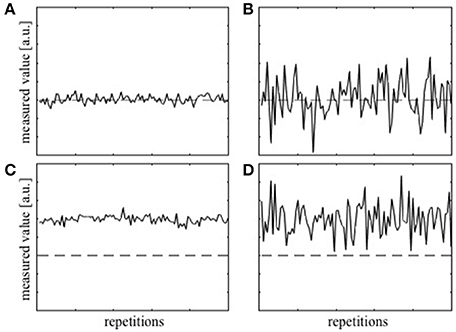
Figure 1. Simulation of repeatedly measured data with (A) high accuracy and high precision, (B) high accuracy, but low precision, (C) low accuracy and high precision, and (D) low accuracy and low precision. The dashed lines represent the true value.

If the transverse magnetization is adequately spoiled before each RF pulse the SPGR signal amplitude is a function of T₁, equilibrium magnetization (M₀), effective transverse relaxation time ($T_2^{*}$), and imaging parameters, i.e., the repetition time (TR), flip angle α and echo time (TE) (Fram et al., 1987)

$\begin{array}{ll}S=Asin\left(\alpha \right)\frac{1-exp\left(-\text{TR}/T_1\right)}{1-cos\left(\alpha \right)·exp\left(-\text{TR}/T_1\right)}& (1)\end{array}$

where $A=S_{0}exp\left(-\text{TE}/T_2^{*}\right)$. Here S₀ is defined as M₀ multiplied by the receive gain of the system and the receive coil sensitivity. Recently, rational approximation of the SPGR signal for small flip angles and short TR was suggested, which provides a simpler form of Equation (1) (Helms et al., 2008),

$\begin{array}{ll}S\cong A\alpha \frac{\text{TR}/T_1}{{\alpha }^2/2+\text{TR}/T_1}& (2)\end{array}$

By acquiring two SPGR signals, S₁ and S₂, at two different flip angles, α₁ and α₂, T₁ estimates can be obtained with a simple algebraic expression (Helms et al., 2008),

$\begin{array}{ll}{T}_1=2\text{TR}\frac{S_1/{\alpha }_1-S_2/{\alpha }_2}{S_2{\alpha }_2-S_1{\alpha }_1}& (3)\end{array}$

Since the VFA method relies on the flip angle dependency of the SPGR signal for T₁ estimation, a correction for $B_1^{+}$ inhomogeneities is necessary in order to obtain unbiased T₁ estimates. The spatially dependent $B_1^{+}$ correction factor, denoted as f_B1, can be determined by normalizing the $B_1^{+}$ map such that 1 is the nominal flip angle. By multiplying α₁ and α₂ by f_B1 in Equation (3) the $B_1^{+}$ bias corrected T₁ equation can be obtained (Helms et al., 2008),

$\begin{array}{ll}{T}_1=2\text{TR}\frac{S_1/{\alpha }_1-S_2/{\alpha }_2}{S_2{\alpha }_2-S_1{\alpha }_1}\frac{1}{f_{B1}^2}& (4)\end{array}$

Measurement of a $B_1^{+}$ map and inclusion of the correction factor, f_B1, in Equation [4] is intended to ensure the accuracy of the T₁ estimates (Stikov et al., 2015). This correction is assumed to correspond to going from Figure 1C to Figure 1A. However, unless the precision of the $B_1^{+}$ map is high, the actual correction may correspond to going from Figure 1D to Figure 1B, or worse going from Figure 1C to Figure 1B thereby lowering the precision of the T₁ estimate.

In the general VFA case, an expression for the variance of the estimated T₁ (${\sigma }_{T_1}^2$) can be calculated for a set of SPGR signals (S₁, S₂, …, and S_N) measured with N different flip angles and a $B_1^{+}$ map (f_B1) (Bevington and Robinson, 2003). Assuming statistically independent measurements of each signal the variance in the T₁ estimate is

$\begin{array}{ll}{\sigma }_{T_1}^2={\displaystyle \sum _{i=1}^N}\left({\sigma }_{S_i}^2{\left(\frac{\partial T_1}{\partial S_i}\right)}^2\right)+{\sigma }_{f_{B1}}^2{\left(\frac{\partial T_1}{\partial f_{B1}}\right)}^2& (5)\end{array}$

where σ_Si and σ_fB1 are the noise levels in S_i and f_B1 respectively. For the VFA T₁ mapping technique proposed by Helms et al. (2008) only two SPGR signals are acquired (N = 2) and T₁ is calculated from Equation (4). Hence the variance of the estimated T₁ propagated from a $B_1^{+}$ map expressed by the second term in Equation (5) is determined by the noise in a $B_1^{+}$ map (σ_fB1) and the partial derivative term which can be obtained from Equation (4):

$\begin{array}{ll}\frac{\partial T_1}{\partial f_{B1}}=\frac{4\text{TR}}{f_{B1}^3}·\frac{S_2{\alpha }_1-S_1{\alpha }_2}{a_1{\alpha }_2\left(S_2{\alpha }_2-S_1{\alpha }_1\right)}& (6)\end{array}$

The T₁ variance propagated from the two SPGR signals can be determined in the same way by the partial derivative terms with respect to S_i:

$\begin{array}{ll}\frac{\partial T_1}{\partial S_1}=\frac{2\text{TR}}{f_{B1}^2}·\frac{S_2\left({\alpha }_2^2-{\alpha }_1^2\right)}{{\alpha }_1{\alpha }_2{\left(S_2{\alpha }_2-S_1{\alpha }_1\right)}^2}& (7)\end{array}$

$\begin{array}{ll}\frac{\partial T_1}{\partial S_2}=\frac{2\text{TR}}{f_{B1}^2}·\frac{-S_1\left({\alpha }_2^2-{\alpha }_1^2\right)}{{\alpha }_1{\alpha }_2{\left(S_2{\alpha }_2-S_1{\alpha }_1\right)}^2}& (8)\end{array}$

Each partial derivative term in Equations (6–8) is a weighting factor for the noise in the corresponding input signal (i.e., S₁, S₂, and f_B1) in Equation (5).

MR Data Collection

Data were collected on four adult volunteers using a 3T MRI scanner (Achieva Platform, Philips Healthcare, Best, The Netherlands). Four different experiments were performed. The first two experiments involved all four volunteers and the input variable f_B1 was repeatedly measured either with small (Experiment 1) or with large spoiler gradients (Experiment 2) to assess two different levels of variance in the $B_1^{+}$ measurements. On one of the volunteers, the other two input variables, S₁ and S₂, were also repeatedly measured (Experiments 3 and 4 respectively) to assess their variances and compare them with the variance introduced by the $B_1^{+}$ measurements.

Before each measurement the scanner performed a full preparatory phase of shimming, center frequency determination and RF transmit power calibration. The repeated measurements approach adopted here captured all noise sources, e.g., thermal/physiological noise, scanner stability, etc. In summary, the four different experiments were designed as follows:

Experiment 1: one S₁, one S₂, and six $B_1^{+}$ maps with small spoiler gradients.

Experiment 2: one S₁, one S₂, and six $B_1^{+}$ maps with large spoiler gradients.

Experiment 3: six S₁, one S₂, and one $B_1^{+}$ map with large spoiler gradients.

Experiment 4: one S₁, six S₂, and one $B_1^{+}$ map with large spoiler gradients.

The 3D SPGR sequence had 0.8 mm isotropic voxels, TR/TE1/TE2/TE3 = 25.0/4.6/11.5/18.3 ms, sensitivity encoding (SENSE) (Pruessmann et al., 1999) factor = 2.0, and scan time = 11.6 min. The SPGR images acquired at three different echo times were averaged to increase the signal-to-noise ratio (SNR) (Helms et al., 2008). The S₁ and S₂ images were acquired with the nominal flip angles of α₁ = 6° and α₂ = 20° respectively, resulting in images with predominantly proton-density (PD) weighting or T₁ weighting. The $B_1^{+}$ maps were acquired at 4.0 mm isotropic resolution using the actual flip angle imaging (AFI) method (Yarnykh, 2007) with either small (A_G1/A_G2=45.33/761.2 mT.ms/m and TR1/TR2/TE = 20/100/2.2 ms) or large (A_G1/A_G2=931.8/1971.0 mT.ms/m, TR1/TR2/TE = 46/138/2.2 ms) spoiler gradients. A_G1 and A_G2 are the spoiler gradient areas on one axis for the interleaved acquisitions with TR1 and TR2, respectively. A nominal flip angle of 60° was used for this AFI $B_1^{+}$ map. To match the scan time (5.2 min) of the AFI acquisitions, the protocol using large spoilers also used a SENSE factor of 1.7. The six repetitions were chosen with consideration of the subject's ability to stay still during the measurements. To ascertain that six repetitions were adequate for a reliable estimate of the variability of input signals, variance was also calculated from the first three, first four and first five repetitions separately. The variance distribution converged after five measurements indicating that the estimate was stable and valid (data not shown).

Data Analysis

All images (S₁, S₂, and the $B_1^{+}$ map) were aligned to the first PD weighted image (i.e., the first of the six S₁ in Experiment 3) using rigid body registration as implemented in SPM8 (Wellcome Trust Centre for Neuroimaging, UCL, UK). The $B_1^{+}$ maps were aligned by using the transformation matrix obtained in the alignment of the corresponding short TR AFI image to the first PD weighted image. Data were evaluated in two different ways to compare the T₁ variances estimated from the in vivo measurements and the theoretical framework:

Experimental variance evaluation: Using Equation (4) six T₁ maps were calculated for each of Experiments 1–4. The voxel-wise variance across these six T₁ maps was then calculated. With this approach, the experimental noise level in the T₁ map, σ_T1,exp, was obtained.

Theoretical variance evaluation: The voxel-wise variance of the repeated S₁, S₂, or $B_1^{+}$ scans (i.e.,${\sigma }_{S_1}^2$, ${\sigma }_{S_2}^2$, or ${\sigma }_{f_{B1}}^2$) was calculated and inserted into the theoretical noise propagation framework [Equations (5–8)], while assuming zero variance for the other two input signals. For example, in Experiment 1 we assumed ${\sigma }_{S_1}^2={\sigma }_{S_2}^2=0$ and evaluated ${\sigma }_{T_1}^2$ by multiplying ${\sigma }_{f_{B1}}^2$ (obtained from the repeated in vivo experiments) by the square of the expression given in Equation (6). ${\sigma }_{T_1}^2$ was similarly evaluated for Experiments 2–4. σ_T1 calculated by this approach is the theoretically-predicted voxel-wise noise level in the T₁ map and is denoted by σ_T1,theo.

Subsequently, coefficient of variation (CV = 100 × standard deviation / mean) maps were calculated to ease comparison of results across Experiments 1–4. Note that CV is inversely proportional to SNR.

The PD weighted image (S₁) was segmented using SPM8 to extract the gray matter (GM) and white matter (WM) segments, which were subsequently thresholded at 0.9 (i.e., 90% probability of belonging to the respective tissue types). The resulting GM and WM masks were used to extract voxel-wise values from the three input images, the T₁ maps and the corresponding CV maps. The median and interquartile range (IQR) of the CV values were then calculated for each tissue type independently.

Results

Example images used to calculate T₁ maps in the work described here, namely two SPGR images (S₁ and S₂) and a $B_1^{+}$ map (in this case with large spoiler gradients) are shown in Figure 2 along with the resulting T₁ map.

FIGURE 2

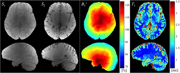
Figure 2. The SPGR images with two different flip angles (S₁ and S₂ in arbitrary units), the $B_1^{+}$ map (in the percentage of nominal flip angle), and the estimated T₁ map (in seconds) are shown from left to right.

Figure 3 provides the results of both methods of variance estimation for Experiments 1–2. Column 1 shows the CV maps calculated from the variance across the repeated $B_1^{+}$ measurements, i.e., ${\sigma }_{f_{B1}}^2$, with small (Figure 3a) and large (Figure 3e) spoiler gradients. The experimental and theoretical evaluations of the noise level in the T₁ map propagated from the variance in the $B_1^{+}$ map (i.e., σ_T1,exp and σ_T1,theo) are shown in column 2 and 3 respectively. Increased spoiling resulted in improved precision of the $B_1^{+}$ maps (compare Figure 3a with Figure 3e), which in turn reduced the variance of the T₁ estimates both experimentally and theoretically (compare Figure 3b with Figure 3f and Figure 3c with Figure 3g). Column 4 shows the percentage difference map between the experimentally-measured (σ_T1,exp) and the theoretically-predicted (σ_T1,theo) noise levels in T₁. In general the discrepancy between σ_T1,exp and σ_T1,theo was small. For Experiment 1 (small spoiler), the mean discrepancies (average of absolute percentage difference values) were 1.97 and 1.44% in GM and WM respectively. For Experiment 2 (large spoiler) these mean discrepancies were reduced to 0.52 and 0.46% respectively. The discrepancy maps (Figures 3a,h) show that, if the noise in the input signal is small, the theoretical prediction works better. This is expected from Equation (5).

FIGURE 3

Figure 3. CV maps of (a,e) the six f_B1 acquired with small and large spoiler gradients in Experiments 1 and 2, (b,f) the noise of the measured T₁ maps (Experimental variance evaluation), and (c,g) the theoretically-predicted noise in the T₁ map from the second term in Equation (5), i.e., $100·{\sigma }_{f_{B1}}·\left(\partial T_1/\partial f_{B1}\right)/{\widehat{T}}_1$ (Theoretical variance evaluation). (d,h) The percentage difference maps between experimentally-measured and theoretically-predicted noise in T₁ estimates. All CV maps shown were calculated by the equations shown in the corresponding gray boxes multiplied by 100. Here, ${\widehat{f}}_{B1}$ and ${\widehat{T}}_1$ represent the means across six f_B1 and corresponding T₁ maps respectively.

Figure 4 shows the results of Experiments 3 and 4 where S₁ and S₂ were measured repeatedly as a comparison to the repeated acquisitions of the $B_1^{+}$ maps. Figure 4a,e show the CV maps across the repeated measurements of S₁ and S₂ (i.e., PD-weighted and T₁-weighted signal respectively). The results of Experimental and Theoretical variance evaluations and the percentage difference map between them are shown in Figures 4b–d,f–h respectively. The mean discrepancies between σ_T1,exp and σ_T1,theo in GM/WM were 0.62/0.37% and 3.03/1.73% for Experiments 3 and 4 respectively. The larger discrepancy between theory and experiment in Experiment 4 (Figure 4h) compared to Experiment 3 (Figure 4d) could be attributed to the larger input noise in the repeated S₂ measurements (Figure 4e) than in the repeated S₁ measurements (Figure 4a). Nonetheless, the fact that the overall discrepancies are small (column 4 of Figures 3, 4) demonstrates the validity of the theoretical framework presented in Equations (5–8) for estimating the variance in T₁ maps measured in vivo.

FIGURE 4

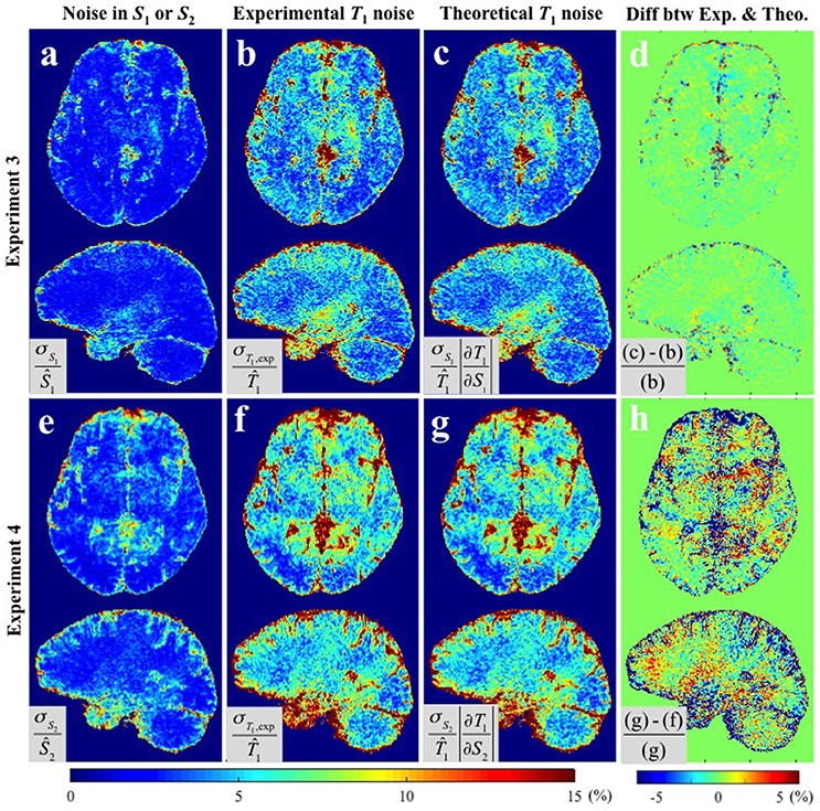
Figure 4. CV maps (a,e) of the input images in Experiments 3 and 4 (S₁ and S₂ respectively), (b,f) the experimentally obtained variability in the estimated T₁ maps using Experimental variance evaluation, and (c,g) the theoretically-predicted T₁ noise from the first term in Equation (5), i.e., $100·{\sigma }_{S_1}·\left(\partial T_1/\partial S_1\right)/{\widehat{T}}_1$ and $100·{\sigma }_{S_2}·\left(\partial T_1/\partial S_2\right)/{\widehat{T}}_1$ respectively (Theoretical variance evaluation). (d) The percentage difference between (b) and (c). (h) The percentage difference between (f) and (g). Results are shown separately for Experiment 3 (a–d) and Experiment 4 (d–h). All CV maps shown were calculated by the equations shown in the corresponding gray boxes multiplied by 100. Ŝ₁, Ŝ₂, and ${\widehat{T}}_1$ in gray boxes denote the average values of six S₁, S₂, and corresponding T₁ maps respectively.

Histograms of the CV maps for GM and WM are shown in Figure 5 from the voxel-wise variance in the input images (solid lines), CV maps obtained with Experimental variance evaluation (dashed lines) or Theoretical variance evaluation (circles) for Experiments 1–4. The histogram of the theoretically-predicted CV values agreed well with that of the experimentally-calculated CV values. Note that the histograms for Experiment 2 (cyan) shifted toward lower CV values and sharpened significantly compared to those for Experiment 1 (red), indicating that the T₁ precision was greatly improved by the increased spoiler gradients, across the entire brain. Except for the distributions from Experiment 1 with small spoiler gradients (solid red) where neither of the distributions from GM nor WM is symmetric, the distributions of CV values in WM are closer to the normal distribution than those in GM.

FIGURE 5

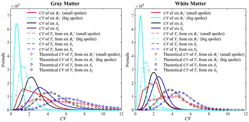
Figure 5. The histograms of CV values for Experiments 1–4 inside GM (left) and WM (right). The solid lines, dashed lines, and circles represent the CV of the six input images, the experimental CV of T₁ calculated from the six input images (Experimental variance evaluation), and the theoretically-predicted CV of T₁ (Theoretical variance evaluation) respectively. The histograms for Experiments 1–4 are shown with red, cyan, black and blue colors, respectively.

Median and IQR values were used to quantitatively summarize the CV histograms given that they were not all normally distributed. Table 1 shows the results for Experiments 1 and 2 on four different subjects and Table 2 for Experiments 3 and 4 on one subject. These results indicate that the noise in S₁, S₂, and f_B1 propagated similarly into the T₁ maps, such that the CV approximately doubled between the input signals and the calculated T₁ maps. Also, the CV values of the T₁ maps calculated via Experimental and Theoretical variance evaluations were similar in both GM and WM. As noted previously, the CV values decreased dramatically going from Experiment 1 with small spoiler to Experiment 2 with large spoiler. This was the case for subjects 1–3 (see Table 1). For subject 4, however, the CV values did not decrease (gray cell background in Table 1). This was likely due to instability in the RF transmit chain and it demonstrates the validity of the theoretical framework for different sources of error.

TABLE 1

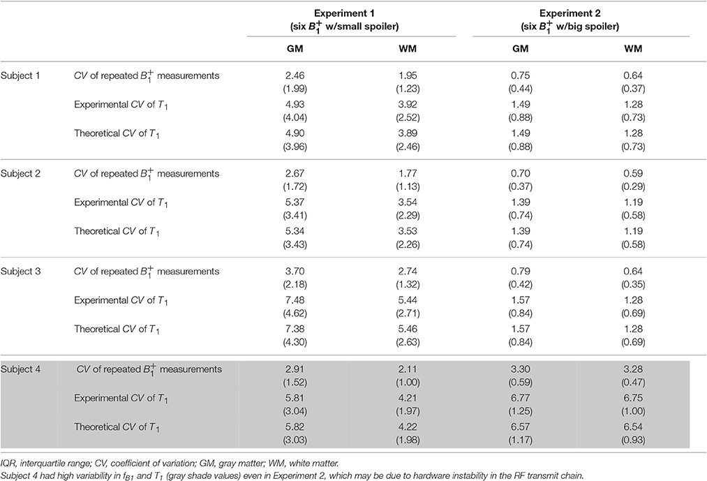
Table 1. Median and (IQR) of CV values inside GM and WM for Experiments 1–2.

TABLE 2

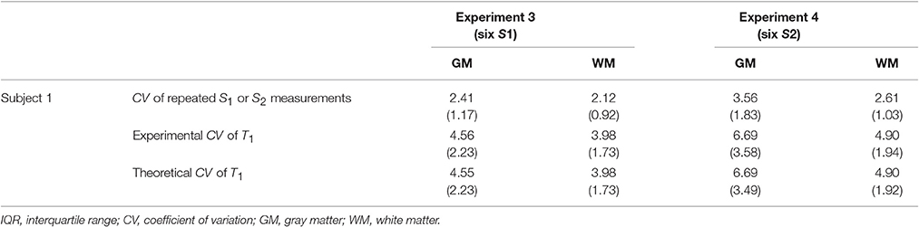
Table 2. Median and IQR of CV values inside GM and WM for Experiments 3–4.

Discussion

Using the VFA method, the precision of T₁ relaxation time measurements depends not only on the SNR of the SPGR images but, crucially, also on the error propagated from the $B_1^{+}$ map that is used to correct the bias caused by spatial inhomogeneity in the achieved flip angle. The precision of the $B_1^{+}$ map is often overlooked as a source of uncertainty in T₁ measurements. Here we have derived analytical solutions for the error propagated to the T₁ relaxation time estimates (Equations 5–8). This analysis indicates that the three signal sources (the two SPGR images with different flip angles and the $B_1^{+}$ map) propagate noise into the T₁ estimates to approximately the same degree, with the CV approximately doubling between each of the three signal sources and the T₁ estimate (Tables 1, 2). By examining two distinct noise levels in the B₁⁺ maps (by manipulating the degree of spoiling), we could show that the precision of the T₁ map can be greatly improved by increasing the precision of the $B_1^{+}$ mapping procedure.

We have experimentally validated the analytical framework by performing repeated experiments to estimate the voxel-wise variance of the T₁ maps. We found overall agreement between the theoretical predictions (σ_T1,theo) and the experimental measures (σ_T1,exp), especially when the input noise, and accordingly T₁ noise, is small as in Experiments 2 and 3. For example, Figure 4d shows discrepancy of less than 1% inside GM and WM and relatively high discrepancy only in voxels containing cerebrospinal fluid (CSF), which we attribute to the fact that CSF has a significantly longer T₁ than GM and WM, for which the VFA sequence was optimized. With higher input noise the discrepancy between theory and measurement tended to increase (Figures 3d, 4h). This is because Equation (5) predicts the propagated error correctly only when σ_Si and σ_fB1 are small enough that the constant slope approximation (i.e., constant partial derivative) is valid over the ranges of σ_Si and σ_fB1 in the S_i/f_B1 vs. T₁ graph. Nonetheless, in the range of experimentally measured noise from our in vivo experiments, the discrepancies were small inside both GM and WM.

Subject 4 had high variability in f_B1 and therefore in the estimated T₁, even in Experiment 2, which used big spoiler gradients to minimize the variance. This may be due to one of the parameters associated with the determination of the RF transmit voltage, which were observed to fluctuate more across the six $B_1^{+}$ acquisitions in subject 4 than across the acquisitions from the other three subjects. This fluctuation might be due to hardware instability in the RF transmit chain. The necessity to keep the RF transmit voltage constant for reliable quantification of T₁ has been reported previously in Lutti and Weiskopf (2013). Therefore, it is reasonable to consider the RF transmit instability as a reason behind the reduced precision of the repeated $B_1^{+}$ map acquisitions in this case. This observation demonstrates that not only the acquisition method, e.g., degree of spoiling used, but also the hardware settings need to be considered when optimizing the precision of $B_1^{+}$, and by extension T₁, measurements.

The CV maps from Experiment 1 had asymmetric left-right distributions as shown in Figures 3a–c for subject 1. While three out of four subjects manifested asymmetric distributions, one of them showed a strong pattern of left-right symmetry (data not shown), indicating that the spatial distribution of precision is subject-specific. This may be due to susceptibility effects from the air-tissue interface, how well the shimming procedure can correct for local field distortions, positioning of the subject in the scanner and interaction with the transmit field. We also found that the histograms of CV values in GM did not tend to be normally distributed compared to those in WM. This may be due to the fact that more GM voxels suffer partial volume effects with CSF and the VFA acquisition was optimized for the T₁ values of GM/WM not the significantly longer T₁ of CSF. The non-normal distributions in the histograms from Experiment 1 for both GM and WM show that the $B_1^{+}$ maps with small spoiler gradients are dominated by noise sources other than thermal noise.

Because the transmit RF field map is smoothly varying, a commonly recommended practice for reducing noise in $B_1^{+}$ maps is spatial smoothing. It must be noted however that systematic offset in a given image cannot be corrected by spatial smoothing. As an example see Figure 6 where the 6 $B_1^{+}$ maps from Experiment 1 were smoothed by a 3D Gaussian kernel with standard deviation of 4 × 4 × 4 mm³. It is evident from the profile extracted from the white line in Figure 6a that spatial smoothing of the 6 individual $B_1^{+}$ maps separately leaves a systematic offset uncorrected (Figures 6c,d). In such cases, when thermal noise does not dominate the error sources but the systematic offset is random in the different repetitions, a more appropriate procedure is averaging multiple acquisitions. Although, repeated measurement of the $B_1^{+}$ map requires additional time, it is usually still the more efficient way to proceed because high-resolution SPGR images take significantly longer to acquire (in our case more than twice as long). This recommendation is further supported by our finding that the $B_1^{+}$ maps propagate approximately the same error as either of the two SPGR images.

FIGURE 6

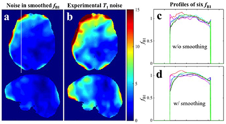
Figure 6. Spatial smoothing effects in Experiment 1 with small spoiler gradients. (a) CV map of the six f_B1 after smoothing. (b) CV map of the six T₁ maps estimated with the six smoothed f_B1 (Experimental variance evaluation). (c,d) Profiles along the white line in (a) for the six original f_B1 maps and six smoothed f_B1 maps respectively.

When optimizing T₁ mapping protocols, previous work has focused mainly on optimizing acquisition parameter settings, most notably the flip angles used to acquire the SPGR images, that minimize uncertainty in the measured T₁ value (Weiss et al., 1980; Wang et al., 1987; Schabel and Morrell, 2009; Helms et al., 2011; Wood, 2015). Although bias resulting from the spatial non-uniformity of the transmit RF transmit field is also well known and is commonly corrected by incorporating a $B_1^{+}$ map into the calculations (Helms et al., 2008; Yarnykh, 2010; Lutti et al., 2013; Stikov et al., 2015), the precision with which the $B_1^{+}$ map is obtained is typically ignored. Pohmann and Scheffler compared the precision of several $B_1^{+}$ mapping methods and found widely varying results depending on the method used and the nominal flip angle to be measured (Pohmann and Scheffler, 2013). Our results further demonstrate the necessity to consider the precision of $B_1^{+}$ mapping when using these to correct bias in the T₁ relaxation time maps. Rather than the assumed high precision estimate of T₁ (Figure 1A), one may arrive at a result that on the average is correct but may also have a high level of uncertainty (Figure 1B). This will have the greatest impact in vivo where there are more sources of noise (e.g., physiologically driven noise) and will reduce the detectable effect size in both cross-sectional and longitudinal studies in which T₁ measurements are used as a biomarker (Lutti et al., 2013).

In this study we used the AFI method for $B_1^{+}$ mapping, which was proposed and optimized by Yarnykh (Yarnykh, 2007, 2010) and has been shown to perform comparatively well (Pohmann and Scheffler, 2013). From Experiments 1–2, we showed that increasing spoiler gradients makes the estimation of T₁ not only more accurate as previously reported (Yarnykh, 2010) but also more precise due to the complete spoiling of the transverse magnetization. Pohmann and Scheffler (2013) found that for a 60° nominal flip angle their implementation of the AFI method had an uncertainty of 3° (5%) in simulations and 4° (7.5%) in phantom experiments. The CV of approximately 3% in the $B_1^{+}$ map that we observed in vivo (Tables 1, 2) is in line with these findings, and may even underestimate the $B_1^{+}$related variance that can be expected to propagate into common T₁ mapping protocols from the map. However, the theoretical framework presented here makes no assumption on the choice of $B_1^{+}$ mapping approach. These findings are equally applicable, regardless of the $B_1^{+}$ mapping method used or how it was optimized to have high precision.

In both the in vivo experimental variance (Experimental variance evaluation) and the theoretical framework (Theoretical variance evaluation) we considered the noise propagating from the three input signals separately (Equations 5–8 and Experiments 1–4). This provides a convenient way in which to compare the effect of the three noise sources on the uncertainty of the final T₁ map. In practice, however, the errors propagating from the three sources are summed (Equation 5). Although CVs for the averaged SPGR signals and the $B_1^{+}$ maps were similar in our in vivo experiments, the precision of $B_1^{+}$ maps can vary significantly depending on the $B_1^{+}$ mapping approach (see for example Figure 6 in Pohmann and Scheffler, 2013), which shows that in phantom measurements some of the $B_1^{+}$ mapping methods, especially the 2D variants, can suffer higher uncertainty for certain acquisition parameter sets). Therefore, neglecting the uncertainty in the $B_1^{+}$ map can lead to significant erroneous overestimation of the precision of the calculated T₁ value.

Also note that including more than two SPGR images with more than two different flip angles for the T₁ estimation may even lead to the increased variability in T₁ since the noise from the additional SPGR images is additive to the total variance in T₁ (${\sigma }_{T_1}^2$) according to Equation (5). This is also reflected by the fact that previous evaluations of uncertainty within the VFA regime conclude that when acquiring additional images the optimal approach is to acquire at the same flip angle and average (Wang et al., 1987; Helms et al., 2011).

To assess the uncertainty in the measurements of SPGR images and $B_1^{+}$ maps we performed repeated in vivo experiments for each of the input images. In such an approach, the uncertainty in each variable includes all sources, e.g., thermal noise, scanner instability, scanner drift, physiological noise and the test/re-test variability (e.g., differences in the optimized shim currents, or power amplifier calibration etc.), whereas usually only the thermal noise components are considered (Cheng and Wright, 2006). Had we simply estimated the thermal noise component by extracting the standard deviation of pixels in the background the theoretically-predicted uncertainty (Theoretical variance evaluation) would have seriously underestimated the uncertainty found in the in vivo T₁ relaxation time measurement (Experimental variance evaluation). In addition we would have confounds due to the Rician noise distribution of magnitude images and the image reconstruction scheme chosen (Constantinides et al., 1997).

A wide array of methods exists for measuring the T₁ relaxation time (Kingsley, 1999). A recently proposed method (Helms et al., 2008) was chosen here because it has been broadly used (Dick et al., 2012; Sereno et al., 2013; Callaghan et al., 2014) and optimized (Helms et al., 2011). However, our findings regarding the dependence of the precision of the T₁ measurement on the level of uncertainty in the $B_1^{+}$ map is not expected to be unique to this method of T₁ relaxation time measurement.

We conclude that when estimating the uncertainty of T₁ mapping methods, the error propagated from the $B_1^{+}$ map must also be considered. Optimizing the SPGR signals while neglecting to improve the precision of the $B_1^{+}$ map will result in a significant underestimation of the final uncertainty in the calculated T₁ relaxation time. Maximizing the precision of the adopted $B_1^{+}$ mapping approach is crucial for studies using T₁ as an imaging biomarker, which require high sensitivity (minimum variance), e.g., to investigate subtle differences in the micro-architectural organization of the brain.

Ethics Statement

This study was carried out in accordance with the recommendations of The Kantonale Ethics Komitee (i.e., regional ethics committee) of Zurich with written informed consent from all subjects. The protocol was approved by The Kantonale Ethics Komitee.

Author Contributions

YL, MC, and ZN designed the study; YL and ZN acquired the data; MC provided software for data analysis; YL, MC, and ZN analyzed data, interpreted the results and wrote the manuscript.

Conflict of Interest Statement

The authors declare that the research was conducted in the absence of any commercial or financial relationships that could be construed as a potential conflict of interest.

Acknowledgments

The Wellcome Trust Centre for Neuroimaging is supported by core funding from the Wellcome Trust 091593/Z/10/Z. ZN and YL were supported by the Swiss National Science Foundation (grant number: 31003A_166118).

References

Bevington, P. R., and Robinson, D. K. (2003). Data Reduction and Error Analysis for the Physical Sciences. Boston, MA: McGraw-Hill.

Google Scholar

Callaghan, M. F., Freund, P., Draganski, B., Anderson, E., Cappelletti, M., Chowdhury, R., et al. (2014). Widespread age-related differences in the human brain microstructure revealed by quantitative magnetic resonance imaging. Neurobiol. Aging. 35, 1862–1872. doi: 10.1016/j.neurobiolaging.2014.02.008

PubMed Abstract | CrossRef Full Text | Google Scholar

Cheng, H. L., and Wright, G. A. (2006). Rapid high-resolution T(1) mapping by variable flip angles: accurate and precise measurements in the presence of radiofrequency field inhomogeneity. Magn. Reson. Med. 55, 566–574. doi: 10.1002/mrm.20791

PubMed Abstract | CrossRef Full Text | Google Scholar

Christensen, K. A., Grant, D. M., Schulman, E. M., and Walling, C. (1974). Optimal determination of relaxation times of fourier transform nuclear magnetic resonance. Determination of spin-lattice relaxation times in chemically polarized species. J. Phys. Chem. 78, 1971–1977. doi: 10.1021/j100612a022

CrossRef Full Text

Constantinides, C. D., Atalar, E., and McVeigh, E. R. (1997). Signal-to-noise measurements in magnitude images from NMR phased arrays. Magn. Reson. Med. 38, 852–857. doi: 10.1002/mrm.1910380524

PubMed Abstract | CrossRef Full Text | Google Scholar

Cunningham, C. H., Pauly, J. M., and Nayak, K. S. (2006). Saturated double-angle method for rapid B1+ mapping. Magn. Reson. Med. 55, 1326–1333. doi: 10.1002/mrm.20896

PubMed Abstract | CrossRef Full Text | Google Scholar

Deoni, S. C. (2007). High-resolution T1 mapping of the brain at 3T with driven equilibrium single pulse observation of T1 with high-speed incorporation of RF field inhomogeneities (DESPOT1-HIFI). J. Magn. Reson. Imaging 26, 1106–1111. doi: 10.1002/jmri.21130

PubMed Abstract | CrossRef Full Text | Google Scholar

Deoni, S. C., Peters, T. M., and Rutt, B. K. (2004). Determination of optimal angles for variable nutation proton magnetic spin-lattice, T1, and spin-spin, T2, relaxation times measurement. Magn. Reson. Med. 51, 194–199. doi: 10.1002/mrm.10661

PubMed Abstract | CrossRef Full Text | Google Scholar

Deoni, S. C., Peters, T. M., and Rutt, B. K. (2005). High-resolution T1 and T2 mapping of the brain in a clinically acceptable time with DESPOT1 and DESPOT2. Magn. Reson. Med. 53, 237–241. doi: 10.1002/mrm.20314

PubMed Abstract | CrossRef Full Text | Google Scholar

Dick, F., Tierney, A. T., Lutti, A., Josephs, O., Sereno, M. I., and Weiskopf, N. (2012). In vivo functional and myeloarchitectonic mapping of human primary auditory areas. J. Neurosci. 32, 16095–16105. doi: 10.1523/JNEUROSCI.1712-12.2012

PubMed Abstract | CrossRef Full Text | Google Scholar

Dowell, N. G., and Tofts, P. S. (2007). Fast, accurate, and precise mapping of the RF field in vivo using the 180 degrees signal null. Magn. Reson. Med. 58, 622–630. doi: 10.1002/mrm.21368

PubMed Abstract | CrossRef Full Text | Google Scholar

Drain, L. E. (1949). A direct method of measuring nuclear spin-lattice relaxation times. Pro. Phys. Soc. Sect. A. 62:301. doi: 10.1088/0370-1298/62/5/306

CrossRef Full Text | Google Scholar

Fram, E. K., Herfkens, R. J., Johnson, G. A., Glover, G. H., Karis, J. P., Shimakawa, A., et al. (1987). Rapid calculation of T1 using variable flip angle gradient refocused imaging. Magn. Reson. Imaging 5, 201–208. doi: 10.1016/0730-725X(87)90021-X

PubMed Abstract | CrossRef Full Text | Google Scholar

Ganter, C. (2006). Steady state of gradient echo sequences with radiofrequency phase cycling: analytical solution, contrast enhancement with partial spoiling. Magn. Reson. Med. 55, 98–107. doi: 10.1002/mrm.20736

PubMed Abstract | CrossRef Full Text | Google Scholar

Haase, A., Frahm, J., Matthaei, D., Hanicke, W., and Merboldt, K. D. (1986). FLASH imaging. Rapid NMR imaging using low flip-angle pulses. J. Magn. Reson. 67, 258–266. doi: 10.1016/0022-2364(86)90433-6

CrossRef Full Text | Google Scholar

Hahn, E. L. (1949). An accurate nuclear magnetic resonance method for measuring spin-lattice relaxation times. Phys. Rev. 76:145. doi: 10.1103/PhysRev.76.145

CrossRef Full Text | Google Scholar

Harkins, K. D., Xu, J., Dula, A. N., Li, K., Valentine, W. M., Gochberg, D. F., et al. (2016). The microstructural correlates of T1 in white matter. Magn. Reson. Med. 75, 1341–1345. doi: 10.1002/mrm.25709

PubMed Abstract | CrossRef Full Text | Google Scholar

Helms, G., Dathe, H., and Dechent, P. (2008). Quantitative FLASH MRI at 3T using a rational approximation of the ernst equation. Magn. Reson. Med. 59, 667–672. doi: 10.1002/mrm.21542

PubMed Abstract | CrossRef Full Text | Google Scholar

Helms, G., Dathe, H., Weiskopf, N., and Dechent, P. (2011). Identification of signal bias in the variable flip angle method by linear display of the algebraic ernst equation. Magn. Reson. Med. 66, 669–677. doi: 10.1002/mrm.22849

PubMed Abstract | CrossRef Full Text | Google Scholar

Insko, E. K., and Bolinger, L. (1993). Mapping of the radiofrequency field. J. Magn. Reson. Ser. A 103, 82–85. doi: 10.1006/jmra.1993.1133

CrossRef Full Text | Google Scholar

Jiru, F., and Klose, U. (2006). Fast 3D radiofrequency field mapping using echo-planar imaging. Magn. Reson. Med. 56, 1375–1379. doi: 10.1002/mrm.21083

PubMed Abstract | CrossRef Full Text | Google Scholar

Kingsley, P. B. (1999). Methods of measuring spin-lattice (T1) relaxation times: an annotated bibliography. Concepts. Magn. Reson. 11, 243–276. doi: 10.1002/(SICI)1099-0534(1999)11:4<243::AID-CMR5>3.0.CO;2-C

CrossRef Full Text | Google Scholar

Liberman, G., Louzoun, Y., and Ben Bashat, D. (2014). T1 mapping using variable flip angle SPGR data with flip angle correction. J. Magn. Reson. Imaging 40, 171–180. doi: 10.1002/jmri.24373

PubMed Abstract | CrossRef Full Text | Google Scholar

Lutti, A., Dick, F., Sereno, M. I., and Weiskopf, N. (2013). Using high-resolution quantitative mapping of R1 as an index of cortical myelination. Neuroimage 93, 176–188. doi: 10.1016/j.neuroimage.2013.06.005

PubMed Abstract | CrossRef Full Text | Google Scholar

Lutti, A., Hutton, C., Finsterbusch, J., Helms, G., and Weiskopf, N. (2010). Optimization and validation of methods for mapping of the radiofrequency transmit field at 3T. Magn. Reson. Med. 64, 229–238. doi: 10.1002/mrm.22421

PubMed Abstract | CrossRef Full Text | Google Scholar

Lutti, A., and Weiskopf, N. (2013). “Optimizing the accuracy of T1 mapping accounting for RF non-linearities and spoiling characteristics in FLASH imaging,” in Proceedings of the 21st Annual Meeting of ISMRM. (Utah, UT).

Nehrke, K., and Börnert, P. (2012). DREAM - A novel approach for robust, ultrafast, multislice B1 mapping. Magn. Reson. Med. 68, 1517–1526. doi: 10.1002/mrm.24158

PubMed Abstract | CrossRef Full Text | Google Scholar

Pohmann, R., and Scheffler, K. (2013). A theoretical and experimental comparison of different techniques for B1 mapping at very high fields. NMR Biomed. 26, 265–275. doi: 10.1002/nbm.2844

PubMed Abstract | CrossRef Full Text | Google Scholar

Preibisch, C., and Deichmann, R. (2009). Influence of RF spoiling on the stability and accuracy of T1 mapping based on spoiled FLASH with varying flip angles. Magn. Reson. Med. 61, 125–135. doi: 10.1002/mrm.21776

PubMed Abstract | CrossRef Full Text | Google Scholar

Pruessmann, K. P., Weiger, M., Scheidegger, M. B., and Boesiger, P. (1999). SENSE: sensitivity encoding for fast MRI. Magn. Reson. Med. 42, 952–962. doi: 10.1002/(SICI)1522-2594(199911)42:5<952::AID-MRM16>3.0.CO;2-S

PubMed Abstract | CrossRef Full Text | Google Scholar

Sacolick, L. I., Wiesinger, F., Hancu, I., and Vogel, M. W. (2010). B1 mapping by bloch-siegert shift. Magn. Reson. Med. 63, 1315–1322. doi: 10.1002/mrm.22357

PubMed Abstract | CrossRef Full Text | Google Scholar

Schabel, M. C., and Morrell, G. R. (2009). Uncertainty in T1 mapping using the variable flip angle method with two flip angles. Phys. Med. Biol. 54:N01. doi: 10.1088/0031-9155/54/1/N01

CrossRef Full Text | Google Scholar

Sereno, M. I., Lutti, A., Weiskopf, N., and Dick, F. (2013). Mapping the human cortical surface by combining quantitative T(1) with retinotopy. Cereb. Cortex. 23, 2261–2268. doi: 10.1093/cercor/bhs213

PubMed Abstract | CrossRef Full Text | Google Scholar

Stikov, N., Boudreau, M., Levesque, I. R., Tardif, C. L., Barral, J. K., and Pike, G. B. (2015). On the accuracy of T1 mapping: searching for common ground. Magn. Reson. Med. 73, 514–522. doi: 10.1002/mrm.25135

PubMed Abstract | CrossRef Full Text | Google Scholar

Venkatesan, R., Lin, W., and Haacke, E. M. (1998). Accurate determination of spin-density and T1 in the presence of rf-field inhomogeneities and flip-angle miscalibration. Magn. Reson. Med. 40, 592–602. doi: 10.1002/mrm.1910400412

PubMed Abstract | CrossRef Full Text | Google Scholar

Wang, H. Z., Riederer, S. J., and Lee, J. N. (1987). Optimizing the precision in T1 relaxation estimation using limited flip angles. Magn. Reson. Med. 5, 399–416. doi: 10.1002/mrm.1910050502

PubMed Abstract | CrossRef Full Text | Google Scholar

Weiss, G. H., Guptaj, R. K., Ferretti, J. A., and Becker, E. D. (1980). The choice of optimal parameters for measurement of spin-lattice relaxation times. I. Mathematical formulation. J. Magn. Reson. 37, 369–379. doi: 10.1016/0022-2364(80)90044-x

CrossRef Full Text | Google Scholar

Wood, T. C. (2015). Improved formulas for the two optimum VFA flip-angles. Magn. Reson. Med. 74, 1–3. doi: 10.1002/mrm.25592

CrossRef Full Text | Google Scholar

Yarnykh, V. L. (2007). Actual flip-angle imaging in the pulsed steady state: a method for rapid three-dimensional mapping of the transmitted radiofrequency field. Magn. Reson. Med. 57, 192–200. doi: 10.1002/mrm.21120

PubMed Abstract | CrossRef Full Text | Google Scholar

Yarnykh, V. L. (2010). Optimal radiofrequency and gradient spoiling for improved accuracy of T1 and B1 measurements using fast steady-state techniques. Magn. Reson. Med. 63, 1610–1626. doi: 10.1002/mrm.22394

PubMed Abstract | CrossRef Full Text | Google Scholar

Zur, Y., Wood, M. L., and Neuringer, L. J. (1991). Spoiling of transverse magnetization in steady-state sequences. Magn. Reson. Med. 21, 251–263. doi: 10.1002/mrm.1910210210

PubMed Abstract | CrossRef Full Text | Google Scholar