 Yueying Zhou
 Limei Zhang1
 Dinggang Shen
- 1School of Mathematics Science, Liaocheng University, Liaocheng, China
- 2College of Electronic and Information Engineering, Shandong University of Science and Technology, Qingdao, China
- 3Department of Radiology and BRIC, University of North Carolina at Chapel Hill, Chapel Hill, NC, United States
- 4Department of Brain and Cognitive Engineering, Korea University, Seoul, South Korea
High-order correlation has recently been proposed to model brain functional connectivity network (FCN) for identifying neurological disorders, such as mild cognitive impairment (MCI) and autism spectrum disorder (ASD). In practice, the high-order FCN (HoFCN) can be derived from multiple low-order FCNs that are estimated separately in a series of sliding windows, and thus it in fact provides a way of integrating dynamic information encoded in a sequence of low-order FCNs. However, the estimation of low-order FCN may be unreliable due to the fact that the use of limited volumes/samples in a sliding window can significantly reduce the statistical power, which in turn affects the reliability of the resulted HoFCN. To address this issue, we propose to enhance HoFCN based on a regularized learning framework. More specifically, we first calculate an initial HoFCN using a recently developed method based on maximum likelihood estimation. Then, we learn an optimal neighborhood network of the initially estimated HoFCN with sparsity and modularity priors as regularizers. Finally, based on the improved HoFCNs, we conduct experiments to identify MCI and ASD patients from their corresponding normal controls. Experimental results show that the proposed methods outperform the baseline methods, and the improved HoFCNs with modularity prior consistently achieve the best performance.
Introduction
Currently, resting state functional magnetic resonance imaging (rs-fMRI), which treats blood oxygen level dependent (BOLD) signals as indirect measures of neural activities, has been widely used in the fields of medicine and neuroscience (Liu et al., 2008; van den Heuvel and Hulshoff Pol, 2010; Liu F. et al., 2013). Based on rs-fMRI, the study of functional connectivity network (FCN) has become a prevalent way to understand brain working mechanism and provide promising biomarkers for diagnosing neural or mental disorders (Bullmore and Sporns, 2009; Fornito et al., 2015; Liu et al., 2017), such as autism spectrum disorder (ASD) (Weng et al., 2010; Wee et al., 2016), Alzheimer's disease (AD) (Wang et al., 2006; Sanz-Arigita et al., 2010), mild cognitive impairment (MCI) (Rombouts et al., 2005; Qiao et al., 2016), major depressive disorder (Greicius et al., 2007; Cullen et al., 2014), schizophrenia (Jafri et al., 2008), and social anxiety disorder (Liu et al., 2015).
To date, researchers have developed many FCN estimation methods (Smith et al., 2011) from the simplest Pearson's correlation (PC) to the most complex dynamic causal modeling. In this paper, we mainly focus on the correlation-based methods due to their relative simplicity and reliability (Smith et al., 2013). Further, we suppose each node of the FCN corresponds to a brain region or a spatial region of interest (ROI) that has been well-defined according to a certain brain atlas, and each “edge” of the FCN corresponds to the relationship between BOLD signals that are extracted from the associated ROIs.
In the conventional correlation-based FCN models, PC is the most popular one for calculating the relationship between ROIs (Smith et al., 2013), but it only captures full correlation without removing the confounding effect from other ROIs. To ease this issue, partial correlations have been employed in calculating the relationship between ROIs for FCN construction (Marrelec et al., 2006). However, the estimation of partial correlation involves the calculation of an inverse covariance matrix, usually resulting in an ill-posed problem. Therefore, many studies adopted a regularizer in the model for more reliable partial correlation estimation (Friedman et al., 2008; Huang et al., 2009; Varoquaux et al., 2010). In fact, the regularizer also plays a role in encoding priors for FCN construction. For example, l1-norm regularizer is commonly used for encoding sparsity prior of FCN (Lee et al., 2011), and also trace norm regularizer is used for low-rank prior (Liu G. et al., 2013; Qiao et al., 2016). In summary, most of the correlation-based FCN models can be formulated by a matrix-regularized learning framework, where different data fitting terms and regularized terms are combined for estimating FCNs. Please see Table 1 in section Related Methods for more details.
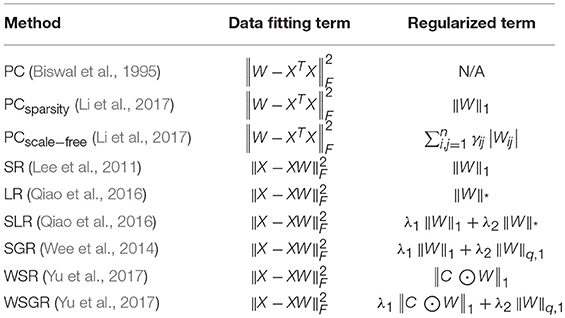
Table 1. Correlation-based FCN estimation methods under a matrix-regularized learning framework, where ||·||F, ||·||1, and ||·||q, 1 denote F-norm, l1-norm, trace norm and lq, 1-norm of a matrix, respectively.
Compared with the aforementioned FCN estimation methods based on low-order correlations, a novel concept of high-order correlation or high-order FCN (HoFCN) has been recently proposed (Chen et al., 2016; Zhang et al., 2016) for measuring more complex interaction information in the brain. Different from the low-order FCN that models the dependency between ROIs, HoFCN aims to capture relationships among different edges. To put it simply, we can consider the ecological chain (network) as an analogy, where the species are regarded as nodes and the ecological chains are the edges between the nodes. In such a way, ecological chains represent the low-order connection information of this network. However, there may exist some relationships among different ecological chains, and the flourishment or destruction of an ecological chain may affect another ecological chain. Therefore, we expect the relationships between edges can provide higher-order information in modeling FCN, compared with the low-order methods that only measure the relationship between nodes.
To date, several studies have suggested that HoFCNs can provide some useful and complementary information for disorder identification (Macke et al., 2011; Plis et al., 2014; Chen et al., 2016; Zhang et al., 2017). For instance, Plis et al. investigated the nonlinear interactions among brain regions in schizophrenia based on mutual information (Plis et al., 2014). Chen et al. proposed to estimate HoFCNs via correlation's correlation, and use a clustering strategy to reduce the dimensionality for efficient computation (Chen et al., 2016, 2017). Guo et al. constructed HoFCN based on minimum spanning tree and applied it for AD classification (Guo et al., 2017). Zhang et al. proposed the hybrid HoFCN for MCI identification based on the linear combination of low- and high-order FCNs (Zhang et al., 2017). Zhao et al. developed the multi-level HoFCN mainly based on PC and applied it for ASD diagnosis (Zhao et al., 2018).
Different from the heuristic methods for defining HoFCNs, Zhou et al. recently proposed to estimate HoFCN based on a rigorous probabilistic framework (Zhou et al., 2018), where a set of low-order correlation matrices (or low-order FCNs) are first calculated separately in sliding windows, and then these correlation matrices are considered as samples for achieving HoFCN by maximum likelihood estimation (MLE). Such a framework not only gives a clear theoretical explanation of HoFCN, but also provides a way of integrating dynamic information encoded in a sequence of low-order FCNs. However, the initially estimated low-order FCNs may be unreliable, since the use of limited volumes/samples in each sliding window will significantly reduce the statistical power. As such, the derived HoFCN may contain noisy connections inheriting from the low-order counterparts. To deal with this problem, we propose to improve the HoFCNs based on a regularized learning framework. To be specific, we adopt a two-step learning strategy. First, an initial HoFCN is estimated using the MLE method as proposed in Zhou et al. (2018). Then, an optimal neighborhood network of the initially estimated HoFCN is learnt to meet the sparsity and modularity regularizers, aiming, respectively to remove possible noisy connections and encode more informative structure (i.e., modularity) of the network. To verify the effectiveness of our proposed method, we apply the improved HoFCNs to identify subjects with MCI and ASD from normal controls (NCs), respectively. The experimental results show that our proposed methods outperform the baseline methods, and the improved HoFCN with modularity prior consistently achieves the best performance.
The rest of this paper is organized as follows. In section Related Methods, we introduce the correlation-based low-order and high-order FCN modeling methods. In section The Proposed Method, we propose our HoFCN learning strategy, including the motivation, model and algorithm. In section Experiments and Results, we evaluate our proposed method with applications to MCI and ASD identification. In section Discussions, we discuss our findings and several aspects that affect the final performance. Then, we conclude the paper in section Conclusion.
Related Methods
In this section, we first summarize the existing correlation-based FCN methods into a matrix-regularized learning framework in Table 1. Then, we specifically describe several representative FCN estimation methods, including PC (Biswal et al., 1995), sparse representation (SR) (Lee et al., 2011) and the MLE-based HoFCN estimation (Zhou et al., 2018).
Pearson's Correlation
As the most popular and simplest method to estimate FCN, PC with its mathematical expression is defined as follows:
where, is the extracted time series from the ith ROI, V is the number of temporal image volumes, P is the total number of ROIs, is the mean of xi, and Wi, j is the correlation weight between the ith and jth ROIs. Without loss of generality, we suppose xiis centralized byand normalized by , and thus we can express PC as , or, its equivalent matrix form
where is the rs-fMRI data matrix.
In practice, we can treat Equation (2) as the solution of the following optimization problem
where ||·||F represents F-norm of a matrix. In this way, we can put PC into the matrix-regularized learning framework reported in Table 1 for a unified understanding.
Sparse Representation
SR is one of commonly-used methods for calculating (regularized) partial correlation. The mathematical model of SR is given as follows:
Similar to PC, it can be rewritten as the following matrix form,
where ||·||F and ||·||1 denote F-norm and l1-norm of the matrix, respectively. The constraint Wii = 0 plays a role in removing xi from X to avoid trivial solution.
Based on the idea of sparsity, many extended SR methods have been developed for constructing FCNs, including sparse group representation (Wee et al., 2014), weighted sparse representation (Yu et al., 2017), weighted sparse group representation (Yu et al., 2017), sparse low-rank representation (Qiao et al., 2016) and sparse PC (Li et al., 2017), to name a few. Most of these methods can be unified in the matrix-regularized leaning framework as shown in Table 1.
MLE-Based HoFCN Estimation
As discussed in section Introduction, many HoFCN estimation methods have been proposed in recent years. Here, we only review the MLE-based method (Zhou et al., 2018) due to its clear probabilistic explanation, and shortly we will use this method (named HoFCNMLE) as a baseline for developing our approach.
The HoFCNMLE method includes two main steps. First, a set of low-order FCNs are estimated in a series of sliding windows. Then, the resulted low-order FCNs are used as samples for estimating HoFCN by MLE with an assumption that the low-order FCN samples follow a matrix-variant normal distribution (Zhang and Schneider, 2010). As a result, the HoFCN, Ω, can be achieved by the following iteration formula (generally, with the identity matrix I as an initial estimation of Ω).
where Wk is the kth low-order FCN associated with the kth sliding window, and is the mean of all the low-order FCNs. Please refer to Zhou et al. (2018) for details of the theoretical formulation and probabilistic explanation.
The Proposed Method
Motivation
As discussed earlier, despite its empirical effectiveness in identifying neuropsychiatric disorders, the typically estimated HoFCN may contain some noisy connections that inherit from the low-order FCNs. In general, the weak connections in HoFCN are removed according to a given threshold, prior to the statistical analysis or classification. However, the thresholding scheme is heuristic and only consider the sparsity aspect of FCN. Therefore, in this section we develop a more flexible approach for improving HoFCN based on the matrix-regularized learning framework, not only aiming to reduce noisy connections of HoFCN, but also introduce more informative structures (i.e., modularity) than just sparsity into HoFCN. In particular, we will consider both sparsity and modularity as the priors of HoFCN, due to their well-accepted neuroscientific basis (Sporns, 2011; Sporns and Betzel, 2016). To our best knowledge, this is the first work to employ the modularity prior in HoFCN estimation.
Model: Learning Neighborhood Networks With Regularizers
For reaching the above goals, we adopt a simple two-step learning strategy. First, we obtain an initial estimation of HoFCN (denoted by Ω0) based on the MLE method as described in section MLE-based HoFCN Estimation. Second, we learn an optimal neighborhood network of the initially estimated HoFCN Ω0 with sparsity and modularity priors, respectively, as regularizers of the objective function.
More specifically, sparsity can usually be encoded by l1-norm regularizer (Lee et al., 2011), and thus the optimal neighborhood network of HoFCN with sparsity prior (named S-HoFCN) can be achieved as follows:
where Ω0 is the initially estimated HoFCN by MLE method, Ω is the improved HoFCN that needs to be sparse and simultaneously keep as the spatial neighbor of Ω0, and μ is the regularized parameter for controlling the balance between the sparsity of Ω and its distance from Ω0.
Furthermore, modularity means that some group structures exist in the network, where the nodes within a group are densely connected, while the nodes between groups are sparsely connected (Sporns and Betzel, 2016). Notably, it has been proved that the modularity of a network can be described by a combination of trace (nuclear) norm and l1-norm under mild conditions (Liu G. et al., 2013; Qiao et al., 2016). Therefore, we optimize the neighborhood network of HoFCN with modularity prior (named M-HoFCN), as follows,
where μ1 and μ2 are regularized parameters used to control the balance between the three terms in the optimization problem. Specially, when μ2 = 0, Equation (8) reduces to S-HoFCN as given in Equation (7), meaning that the sparsity is a necessary but not sufficient condition for modularity. Note that the proposed models in both Equations (7, 8) are also fit for matrix-regularized learning framework described in Table 1.
Algorithm
Here, we only give the optimization algorithm for solving M-HoFCN, since S-HoFCN is a special case of M-HoFCN. Note that the objective function in Equation (8) is convex, but the l1-norm and trace norm are both indifferentiable. To address this kind of optimization problem, a number of algorithms have been developed in the machine learning community (Tomioka and Sugiyama, 2009; Richard et al., 2012; Zhuang et al., 2012; Oymak et al., 2014). We choose the proximal method (Combettes and Pesquet, 2009; Bertsekas, 2012) to solve Equation (8), due to its simplicity and efficiency.
In particular, we first consider the data fitting term in Equation (8). Since it is differentiable, we can calculate its gradient with respect to Ω, and get ∇f(Ω) = 2(Ω−Ω0). As a result, we have the gradient descent step as follows,
where αk is the step size.
Then, according to the definition of proximal operator (Combettes and Pesquet, 2009), the proximal operator of l1-norm (i.e., μ1|| Ω||1) is given as follows,
where sgn(·) and abs(·) are sign and absolute functions, respectively. Equation (10) in fact imposes a soft-threshold operation on the entries of Ω. Similarly, the proximal operator of trace norm is equivalent to a shrinkage operation on the singular value of Ω (Ji and Ye, 2009), as follows.
where is the singular value decomposition of matrix Ω.
Finally, to circumvent the case that the current Ωk moves out of the “feasible region” regularized by l1-norm || Ω||1 and trace norm , we use the proximal operations proxμ1||·||1 and on Ωk, respectively, as given in Equations (10, 11). Hence, we get a simple algorithm to solve Equation (8) as shown in Table 2.
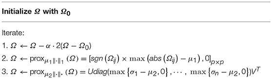
Table 2. Algorithm for solving M-HoFCN in Equation (8).
Experiments and Results
In this section, we first evaluate the proposed method by identifying subjects with MCI from NCs based on ADNI dataset (http://adni.loni.ucla.edu), and then conduct an ASD identification task based on ABIDE database (http://fcon_1000.projects.nitrc.org/indi/abide/) for further illustrating the generalization of the proposed method.
Data Acquisition and Preprocessing
For MCI identification, 137 subjects (including 68 MCIs and 69 NCs) were selected in our study. The subjects were age-matched and scanned by 3.0T Philips scanners. SPM8 (http://www.fil.ion.ucl.ac.uk/spm/) toolbox was used to process the acquired rs-fMRI data. For each subject, the scanning time was 7 min, corresponding to 140 volumes. Subjects with more than 2.5 min of large framewise displacement (FD > 0.5) were excluded before data inclusion. To keep signal stabilization, the first 3 volumes of each subject were also removed, and the remaining volumes were corrected for subsequent analysis. During the scan, a rigid-body transformation was applied to correct head motion, and the subjects with head motion larger than 2 mm or 2° were excluded. The rs-fMRI images were registered to the Montreal Neurological Institute (MNI) space and spatially smoothed by a Gaussian kernel with full width at half maximum of 6 × 6 × 6 mm3. To further reduce the influences of nuisance signals, regression of ventricle and white matter signals as well as Friston 24-parameter model (Friston et al., 1996) were also performed. Using Automated Anatomical Labeling (AAL) template (Tzourio-Mazoyer et al., 2002), the pre-processed BOLD signals were divided into 116 ROIs, among which 90 ROIs are in the cerebra and the rest 26 are in the cerebella. For each ROI, prior to FCN estimation, its mean rs-fMRI time series was band-pass filtered from 0.015 to 0.15 Hz. At last, all the mean time series of the whole brain were put into a data matrix X∈R137 × 116.
For ASD identification, we use the same preprocessed dataset as in Wee et al. (2016). Specifically, 92 subjects including 45 ASD patients and 47 typically developing NCs (with ages between 7 and 15 years old) from this dataset are selected. All rs-fMRI images were acquired using a standard echo-planar imaging sequence on a clinical routine 3T Siemens Allegra scanner. During 6 min rs-fMRI scanning procedure, the subjects were required to relax with their eyes focusing on a white fixation cross in the middle of the black background screen projected on a screen. The imaging parameters include the flip angle as 90°, 33 slices, TR/TE as 2000/15 ms with 180 volumes, and 4.0 mm voxel thickness. The fMRI data were preprocessed by SPM8. Specifically, the first 10 rs-fMRI volumes of each subject were discarded. The remaining volumes were calibrated as follows: (1) normalization to MNI space with resolution 3 × 3 × 3 mm3; (2) regression of nuisance signals (ventricle, white matter, global signals, and head-motion) with Friston 24-parameter model; (3) band-pass filtering (0.01–0.08 Hz); (4) signal de-trending. After that, the BOLD time series signals were partitioned into 116 ROIs, according to the AAL atlas. At last, we put these time series into a data matrix X∈R170 × 116.
FCN Construction
With the preprocessed rs-fMRI data, we calculate the improved HoFCNs using the proposed S-HoFCN and M-HoFCN methods, respectively. Moreover, for comparison, we construct FCNs based on the baseline methods including PC, SR and HoFCNMLE.
In Figure 1, we show the adjacency matrices of a certain FCN constructed by five different methods for MCI identification. The regularized parametric values used in SR, S-HoFCN and M-HoFCN are λ = 24, μ = 2−3 and ,, respectively. For the high-order methods, the width of sliding windows is fixed to N = 70, and step size s = 1. As seen from Figure 1, the networks based on PC and HoFCNMLE are dense, meaning that both low-order and high-order correlations without sparsity constraints may cause some “noisy” connections. In contrast, the networks based on SR, S-HoFCN, and M-HoFCN are sparse due to the introduction of l1-norm regularizer. Further, we note that M-HoFCN shows clearer modular structures than S-HoFCN, since the combination of l1-norm and trace norm regularizers has been proved to result in modularity (Qiao et al., 2016). Finally, it is observed that the high-order FCNs shown in Figures 1C–E tend to have more fine-grained modularity than the low-order FCNs shown in Figures 1A,B, which is consistent with the conclusion that the HoFCNs may be able to capture more subtle network structures as discussed in Zhang et al. (2016).
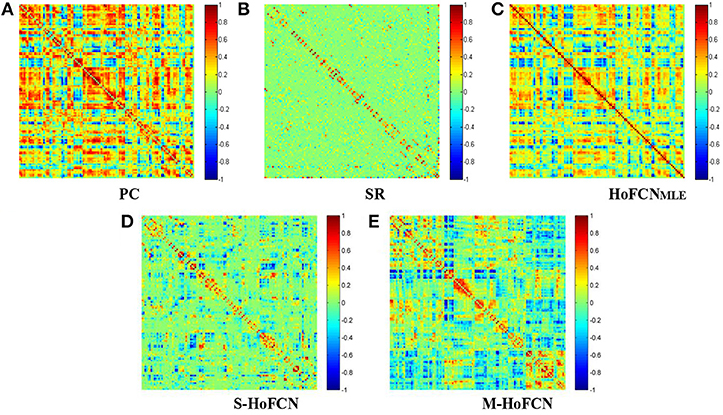
Figure 1. The FBN adjacency matrices constructed by five different methods. (A) PC, (B) SR, (C) HoFCNMLE, (D) S-HoFCN, and (E) M-HoFCN.
Feature Selection and Classification
In our experiments, we adopt the edge weights of FCN or HoFCN as features for MCI/ASD identifications. Although the edge weights include the full information of the networks, it typically causes the curse of dimensionality, since the number of feature dimension, i.e., 116 × (116−1)/2 = 6670, is far greater than the sample size (i.e., the number of subjects). To address this problem, we first employ the two-sample t-test (p = 0.05) to select features before MCI/ASD classifications.
We use the linear support vector machine (SVM) (Chang and Lin, 2011) with default C = 1 for conducting the classification task. A leave-one-out cross validation (LOOCV) is adopted in our experiments to estimate the classification performance of different methods. It works in a way that in each run only one of T samples (subjects) is adopted for testing while the rest T−1 samples are used for training a classifier. Therefore, we can obtain the final performance by averaging results of all the runs.
In general, one or more hyperparameters are involved in the FCN estimation methods. Specifically, for the regularization parameters (i.e., λ in SR, μ in S-HoFCN and μ1, μ2 in M-HoFCN), we conduct a line or grid search in the range of (2−5, 2−4, ⋯, 20, ⋯, 24, 25). Note that no such parameters are involved in PC and HoFCNMLE. For a fair comparation, we introduce a thresholding parameter into PC and HoFCNMLE to sparsify the initially estimated FCNs by removing the weakly connected edges. To be consistent, we employ 11 threshold values that correspond to different levels of sparsity (1%, 10%, ⋯, 90%, 100%) for PC and HoFCNMLE. For example, 10% means that the threshold value is set to remove 90% edges from the FCN, while 100% means all edges are preserved.
To obtain the optimal parameters for each method, we use an inner LOOCV procedure on the training data. Given a parametric value, in the current T−1 training samples for the classification task, we use T−2 samples to select features (t-test with p = 0.05) and train a classifier (SVM with C = 1), while the rest one to validate the performance of the trained classifier. Once the best validation performance is achieved by averaging the accuracies of all the inner LOOCV runs, we can determine the optimal value of the parameter for the current training samples. It is worth noting that there are sliding window parameters used in estimating the initial HoFCNs. We will have a detailed discussion about this problem in Section Sensitivity to Network Modeling Parameters.
In Figure 2, we display the pipeline of MCI identification used in our experiments. Based on the preprocessed fMRI data, we first estimate the initial HoFCNs based on the MLE method, and then improve the initially estimated HoFCNs by introducing sparsity and modularity priors, respectively. Finally, we apply the improved HoFCNs to identify patients suffering from MCI or ASD via the LOOCV scheme.
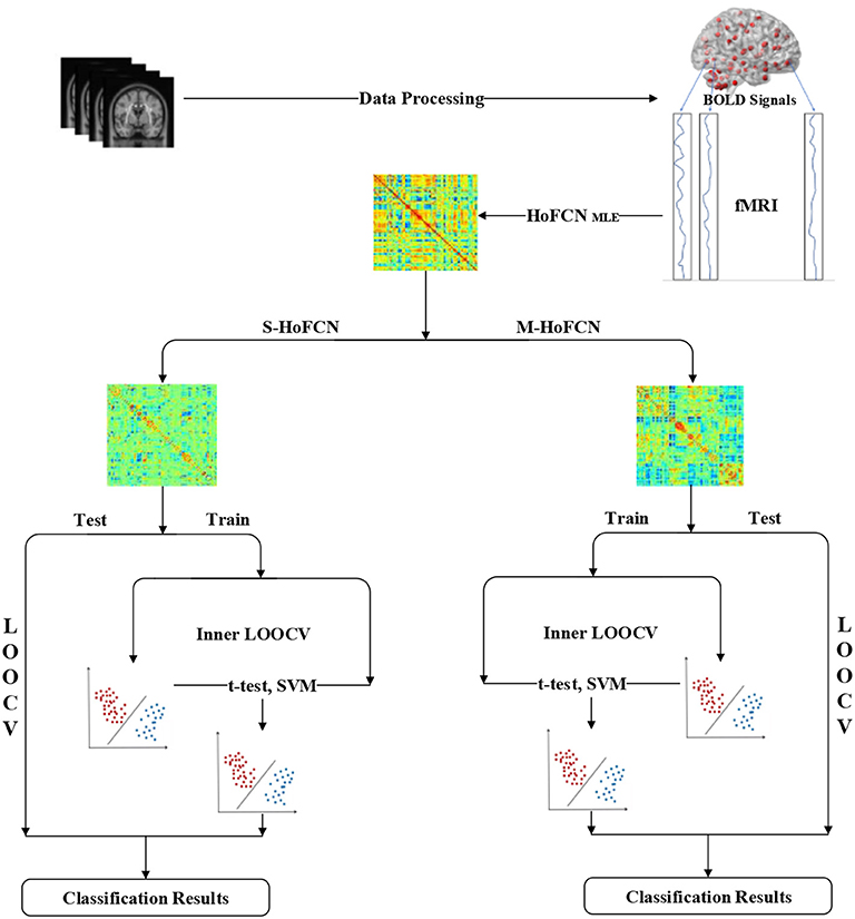
Figure 2. The pipeline of MCI/ASD identifications used in this study.
To evaluate the different FCN estimation methods, we adopt accuracy (ACC), sensitivity (SEN) and specificity (SPE) (Sokolova et al., 2006) as performance metrics. Their definitions are given in Table 3, where TP, TN, FP, and FN indicate true positive, true negative, false positive and false negative, respectively. Of note, in this work, we treat MCI/ASD patients as the positive class while the NCs as the negative.
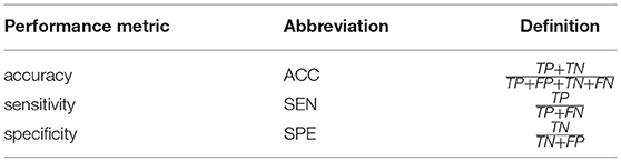
Table 3. Definitions of the performance metrics involved in this paper.
Classification Results
In Table 4, we report the classification results of five different methods for MCI classification task. For the three HoFCN methods, we report the best result based on different sizes of sliding windows (N = 50, s = 1 for HoFCNMLE; N = 70, s = 2 for S-HoFCN; and N = 70, s = 6 for M-HoFCN). As shown in Table 4, with respect to ACC and SPE, the proposed methods outperform the baseline methods, and they are consistently better than HoFCNMLE. Especially for M-HoFCN, it achieves the best performance. Therefore, we argue that the modularity prior is of vital importance in removing the noisy connections and improving the reliability of HoFCNs. However, we note that, in terms of SEN, the proposed methods do not work well. In the next section, we will further investigate this phenomenon.
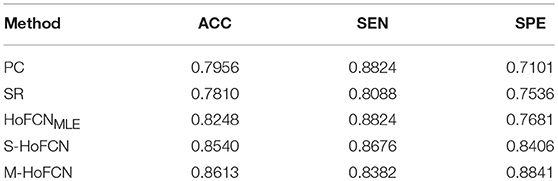
Table 4. The classification results based on five different methods for MCI identification, with N = 50, s = 1 for HoFCNMLE, N = 70, s = 2 for S-HoFCN, and N = 70, s = 6 for M-HoFCN.
In Table 5, we simply report the best experimental results of ASD identification. For three HoFCN methods, s is fixed with 1, while N = 90, 110, 70 for HoFCNMLE, S-HoFCN, and M-HoFCN, respectively. In terms of ACC, the proposed methods perform better than low-order FCNs, and better than the results reported in Wee et al. (2016). Similar to the results on MCI dataset, the M-HoFCN method also achieves the best performance, meaning that the modularity prior plays an important role in FCN modeling.
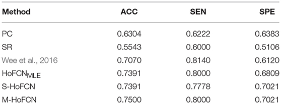
Table 5. Comparison of the best classification results based on six different methods for ASD identification. Here, we empirically fix s = 1, and N = 90, 110, 70 for HoFCNMLE, S-HoFCN and M-HoFCN, respectively.
Discussions
Sensitivity to Network Modeling Parameters
In this study, the involved parameters can be divided into two groups, i.e., sliding window parameters of HoFCNs and the regularization parameters (or threshold values) in the network estimation models. As discussed earlier, we have selected the optimal regularized parameter via inner LOOCV. In the following, we will discuss the sensitivity to the parameters of sliding windows (i.e., width N and step size s) of three HoFCN methods (HoFCNMLE, S-HoFCN and M-HoFCN). To this end, we conduct experiments for MCI/ASD identifications under three cases:
Case 1: Varied window widths N = 50, 70, 90, 110 and fixed step size s = 1 for MCI identification. Figure 3 shows the classification results of three HoFCN methods under this case. (Of note, in both Figures 3–5, we simply use MLE, S and M to represent the corresponding HoFCNMLE, S-HoFCN and M-HoFCN methods, respectively.) It can be observed that our proposed methods perform better than HoFCNMLE and have the best performance at N = 70. For ACC, M-HoFCN has 100% possibilities to outperform HoFCNMLE, and 75% possibilities to outperform S-HoFCN. For SEN and SPE, M-HoFCN has 75% possibilities to work better than HoFCNMLE. That is, M-HoFCN is the best method for MCI classification. Additionally, we note that the bigger value of N tends to result in worse performance, which is consistent with the finding of choosing window sizes in Hindriks et al. (2016).
Case 2: Fixed window width N = 70 and varied step sizes s = 1, 2, 4, 6, 8 for MCI identification. We choose N = 70 since, as shown in Figure 3, the HoFCN methods tend to have the best performance at 70. In this way, we show classification results based on three HoFCN methods in Figure 4. By comparison, for ACC, the proposed methods have 100% possibilities to outperform HoFCNMLE, and M-HoFCN has 80% possibilities to outperform S-HoFCN; for SEN and SPE, S-HoFCN and M-HoFCN both have 80% possibilities to perform better than HoFCNMLE. As such, our proposed methods at least have 80% possibilities that perform better than HoFCNMLE, and M-HoFCN has the best performance at N = 7 0, s = 6, while S-HoFCN at N = 70, s = 2. By using the fixed window width N = 70, we find that the performances of three HoFCN methods with varied step sizes are relatively stable.
Case 3: Varied window widths N = 50, 70, 90, 110, 130 and fixed s = 1 for ASD identification. As shown in Figure 5, S-HoFCN has 80% possibilities to work better than HoFCNMLE for ACC and SPE, and 60% for SEN; M-HoFCN has 100% possibilities to outperform HoFCNMLE for SPE, and 60% for ACC and SEN. For different methods, HoFCNMLE gets the best performance at N = 90, while S-HoFCN at N = 110 and M-HoFCN at N = 70. Compared with the performance of three HoFCN methods, we found that M-HoFCN averagely achieves the best performance and it remains more stable than the other two methods. It is consistent with the finding in MCI identification.
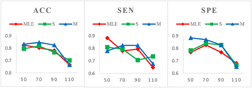
Figure 3. Comparison of classification results based on three HoFCN methods for MCI identification, with varied window widths N = 50, 70, 90, 110 and fixed step size s = 1. The proposed methods (especially M-HoFCN) are consistently better than HoFCNMLE, and they tend to have the best classification performance at N = 70.
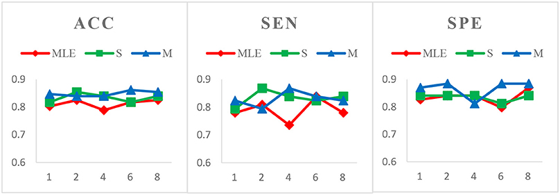
Figure 4. Comparison of classification results based on three HoFCN methods for MCI identification, with different step size s = 1, 2, 4, 6, 8 and fixed window width N = 70. Our proposed methods have 80% possibilities to perform better than HoFCNMLE.
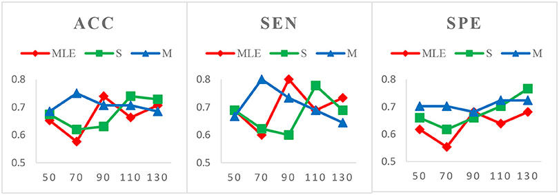
Figure 5. Comparison of classification results based on three HoFCN methods for ASD identification, with varied N = 50, 70, 90, 110, 130 and fixed s = 1. Note that M-HoFCN achieves the best performance in average.
Parcellation of the Brain
We adopt AAL atlas with 116 ROIs as network nodes in this work. To date, there exists different ROI definitions in different brain anatomical/functional templates, such as AAL, Harvard-Oxford (http://www.fmrib.ox.ac.uk/fsl/), Eickhoff-Zilles (Eickhoff et al., 2005) and Automatic Non-linear Imaging Matching and Anatomical Labeling (ANIMAL) (Collins et al., 1995; Wang et al., 2009), etc. As reported in Wang et al. (2009), AAL and ANIMAL templates can lead to significant differences in network topological properties. Craddock et al. also revealed that ROI size had great impact on the network performance analysis, and 200 ROIs can offer better interpretability (Craddock et al., 2012). Therefore, we further conduct experiments for constructing FCNs with 200 ROIs from (Craddock et al., 2012), and take ASD classification as an example for evaluating the influence of different parcellation schemes on the final accuracy. Experimental results show that the proposed M-HoFCN still achieves the best ACC (0.6923), compared with PC (0.6248), SR (0.5167), HoFCNMLE (0.6811), and S-HoFCN (0.6730), which further illustrates the importance of using modularity prior in FCN estimation. Note, however, that the performance of most methods reduces greatly with 200 ROIs. The possible reason is that 200 ROIs, resulting in 200 × (200−1)/2 = 19900 edges, cause the challenge for feature selection or the “curse of dimensionality,” since limited training samples are involved. In the future, we plan to further investigate the influence of differently selected templates on the network properties and the subsequent classification performance.
Head Motion Artifacts
As we know, the FCN estimation based on rs-fMRI data is sensitive to the head motion (Van Dijk et al., 2012; Power et al., 2014). To eliminate the influence of head motion artifacts, a commonly used method is data scrubbing that removes some volumes based on FD or DVARS (Power et al., 2012). However, in this study, we did not perform scrubbing operation to exclude volumes since dynamic information is necessarily encoded by the sliding window scheme for estimating initial low-order FCNs. The removal of volumes would disrupt the autocorrelation structure of data, which is problematic related to temporal filtering and dynamic information encoding (Janine et al., 2017). In fact, several related studies (Chen et al., 2016, 2017) also did not suggest scrubbing operation due to the same reason. Additionally, the data scrubbing often removes relatively high amount of data, thus reducing the statistical power, and, in practice, how to determine a suitable threshold of FD is still an open problem.
To further study the impact of head motion artifacts on the classification performance, we conduct the network modeling methods without regression of Friston 24-parameters. With fixed parameters such as N = 70 and s = 1, the experimental ACCs for ASD identification are PC (0.6750), SR (0.6104), HoFCNMLE (0.6511), S-HoFCN (0.6430), and M-HoFCN (0.6458), respectively. Compared with the results in Table 5, we note that most of the methods tend to decrease ACC, meaning that head motion artifacts have a significant influence on the classification performance. In other words, regressing out the head motion artifacts can contribute to achieve better (at least more discriminative) FCNs.
Top Discriminative Features
As previously mentioned in section Feature Selection and Classification, we adopt the edge weights of estimated FCN as features for classification. Here, we use two-sample t-test to re-select the features for MCI and ASD identification problems, respectively, based on the proposed M-HoFCN method, since it achieves the best performance. In particular, after constructing FCNs by M-HoFCN model (N = 70, s = 6 for MCI; and N = 70, s = 1 for ASD), we apply t-test to select discriminative features in order of their p-values (<0.001). In this way, we select 72 and 67 discriminative features for MCI and ASD identification tasks, respectively, and visualize the features in Figure 6. Of note, the thickness of each arc represents the discriminative power that is inversely proportional to the corresponding p-value.
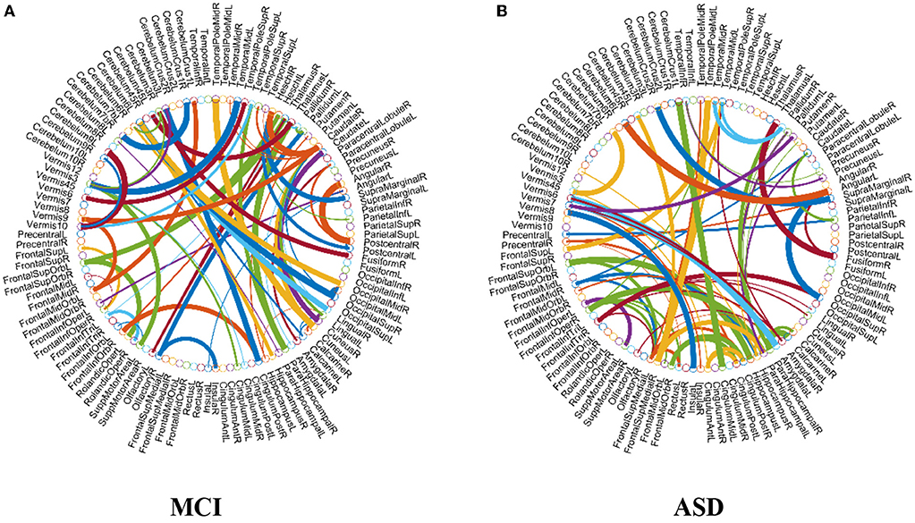
Figure 6. The most discriminative features (network connections) involved in the classification tasks by using t-test with p < 0.001. Note that the thickness of the arcs is inversely proportional to the corresponding p-value for indicating the discriminative power of the features. (A) MCI and (B) ASD.
From Figure 6A, we found that the top discriminative features (i.e., functional connections) and their corresponding brain regions include right inferior frontal gyrus, bilateral hippocampus, bilateral parahippocampal gyrus, right pallidum, right caudate, left middle temporal gyrus, left cerebellum 6, etc. The findings are partially consistent with previous studies (Wolf et al., 2003; Albert et al., 2011; Solodkin et al., 2013). In particular, the right inferior frontal gyrus (Salvatore et al., 2015), bilateral hippocampus (Chen et al., 2016), bilateral parahippocampal gyrus (Echávarri et al., 2011), right pallidum (Supekar et al., 2008; Albert et al., 2011), right caudate (Albert et al., 2011), left middle temporal gyrus (Kosicek and Hecimovic, 2013; Chen et al., 2016), and left cerebellum 6 (Suk et al., 2015) are all reported as potential biomarkers for MCI or AD identification. However, currently it is an open problem for explaining these FCN-based biomarkers. In the future, we plan to provide further experimental evidences toward the biological explanation of those involved functional connectivity or brain regions.
In terms of the selected features as shown in Figure 6B, brain regions that may contribute to ASD identification in this work include the left precentral gyrus, right middle frontal gyrus, right hippocampus, bilateral parahippocampal gyrus, right amygdala, bilateral putamen, left caudate, bilateral pallidum, and bilateral middle temporal, many of which are widely reported in the previous studies associated with ASD identification (Sparks et al., 2002; Haznedar et al., 2006; Rojas et al., 2006; Toal et al., 2009; Ecker et al., 2010; Qiu et al., 2010).
Limitations
In this work, we only use PC as a cornerstone in construction of HoFCN due to its simplicity and popularity. However, as we described above, PC can only capture the full correlation, and thus partial correlation-based methods such as SR may be considered in practice. Besides, many researchers have devoted their efforts to FCN estimation methods based on group analysis. For example, Liu et al. proposed a hierarchical Markov random field model to capture both group and subject FCNs simultaneously, which can take within-subject coherence and between-subject consistency of the network label maps into account (Liu et al., 2014); Ghanbari et al. designed a multi-layer graph clustering algorithm to extract hub-networks by non-negative matrix factorization and applied the hubs to characterize population commonalities and subject variations between ASD and typically developing children (Ghanbari et al., 2017); Kam et al. proposed a multiple FCN model using hierarchical clustering and applied it for ASD diagnosis (Kam et al., 2017). These methods provide a different understanding toward brain structure and group/subject analysis, which we can consider in our future studies.
Conclusion
In this paper, we develop an effective way of improving HoFCN estimation, by learning a neighborhood networks of the initial HoFCN with sparsity and modularity priors as regularizers, respectively. We apply our proposed methods to identify subjects with MCI and ASD from their corresponding NCs. In both MCI and ASD identifications, our proposed HoFCN methods consistently outperform the baseline methods. Especially, the M-HoFCN tends to achieve the best performance, which illustrates the importance of the modularity prior in FCN estimation.
Author Contributions
DS put forward the idea of HoFCN and provided the preprocessed rs-fMRI data. LQ and YZ proposed to learn the neighborhood networks that meet sparsity and modularity for improved HoFCN estimation. YZ, LZ, and ST designed the procedures of MCI/ASD identification experiments. All authors developed the estimation algorithm and contributed to the preparation of the article, figures, and tables.
Conflict of Interest Statement
The authors declare that the research was conducted in the absence of any commercial or financial relationships that could be construed as a potential conflict of interest.
Acknowledgments
We thank Yining Zhang for the insightful and helpful discussions. This work is partly supported by National Natural Science Foundation of China (61402215), and Natural Science Foundation of Shandong Province (ZR2018MF020).
References
Albert, M. S., DeKosky, S. T., Dickson, D., Dubois, B., Feldman, H. H., Fox, N. C., et al. (2011). The diagnosis of mild cognitive impairment due to Alzheimer's disease: recommendations from the national institute on Aging-Alzheimer's Association workgroups on diagnostic guidelines for Alzheimer's disease. Alzheimers Dement. 7, 270–279. doi: 10.1016/j.jalz.2011.03.008
Bertsekas, D. P. (2012). “Chapter 4: Incremental gradient, subgradient, and proximal methods for convex optimization: a survey,” in Optimization for Machine Learning (Cambridge, MA; London: MIT Press).
Biswal, B. B., Yetkin, F. Z., Haughton, V. M., and Hyde, J. S. (1995). Functional connectivity in the motor cortex of resting human brain using echo-planar MRI. Magn. Reson. Med. 34, 537–541. doi: 10.1002/mrm.1910340409
Bullmore, E., and Sporns, O. (2009). Complex brain networks: graph theoretical analysis of structural and functional systems. Nature Rev. Neurosci. 10, 186–198. doi: 10.1038/nrn2575
Chang, C. C., and Lin, C. J. (2011). LIBSVM: a library for support vector machines. ACM Trans. Intell. Syst. Technol. 2, 1–27. doi: 10.1145/1961189.1961199
Chen, X., Zhang, H., Gao, Y., Wee, C. Y., Li, G., and Shen, D. (2016). High-order resting-state functional connectivity network for MCI classification. Hum. Brain Mapp. 37, 3282–3296. doi: 10.1002/hbm.23240
Chen, X., Zhang, H., Lee, S. W., and Shen, D. (2017). Hierarchical high-order functional connectivity networks and selective feature fusion for MCI classification. Neuroinformatics 15, 1–14. doi: 10.1007/s12021-016-9321-x
Collins, D. L., Holmes, C. J., Peters, T. M., and Evans, A. C. (1995). Automated 3D modelbased neuroanatomical segmentation. Human brain mapping 3. Hum. Brain Mapp. 3, 190–208. doi: 10.1002/hbm.460030304
Combettes, P. L., and Pesquet, J. C. (2009). “Chapter 10: Proximal splitting methods in signal processing,” in Fixed-Point Algorithms for Inverse Problems in Science and Engineering, Springer Optimization and Its Applications, Vol. 49, ed H. H. Bauschke (New York, NY: Springer Science+Business Media), 185–212. doi: 10.1007/978-1-4419-9569-8_10
Craddock, R. C., James, G. A., Hu, X. P., and Mayberg, H. S. (2012). A whole brain fMRI atlas generated via spatially constrained spectral clustering. Hum. Brain Mapp. 33, 1914–1928. doi: 10.1002/hbm.21333
Cullen, K. R., Westlund, M. K., Klimes-Dougan, B., Mueller, B. A., Houri, A., Eberly, L. E., et al. (2014). Abnormal amygdala resting-state functional connectivity in adolescent depression. JAMA Psychiatry 71, 1138–1147. doi: 10.1001/jamapsychiatry.2014.1087
Echávarri, C., Aalten, P., Uylings, H. B., Jacobs, H. I., Visser, P. J., Gronenschild, E. H., et al. (2011). Atrophy in the parahippocampal gyrus as an early biomarker of Alzheimer's disease. Brain Struct. Funct. 215, 265–271. doi: 10.1007/s00429-010-0283-8
Ecker, C., Rocha-Rego, V., Johnston, P., Mourao-Miranda, J., Marquand, A. F., Daly, E., et al. (2010). Investigating the predictive value of whole-brain structural MR scans in autism: a pattern classification approach. Neuroimage 49, 44–56. doi: 10.1016/j.neuroimage.2009.08.024
Eickhoff, S. B., Stephan, K. E., Mohlberg, H., Grefkes, C., Fink, G. R., Amunts, K., et al. (2005). A new SPM toolbox for combining probabilistic cytoarchitectonic maps and functional imaging data. Neuroimage 25, 1325–1335. doi: 10.1016/j.neuroimage.2004.12.034
Fornito, A., Zalesky, A., and Breakspear, M. (2015). The connectomics of brain disorders. Nat. Rev. Neurosci. 16, 159–172. doi: 10.1038/nrn3901
Friedman, J., Hastie, T., and Tibshirani, R. (2008). Sparse inverse covariance estimation with the graphical lasso. Biostatistics 9, 432–441. doi: 10.1093/biostatistics/kxm045
Friston, K. J., Williams, S., Howard, R., Frackowiak, R. S., and Turner, R. (1996). Movement-related effects in fMRI time-series. Magn. Reson. Med. 35, 346–355. doi: 10.1002/mrm.1910350312
Ghanbari, Y., Bloy, L., Tunc, B., Shankar, V., Roberts, T. P. L., Edgar, J. C., et al. (2017). On characterizing population commonalities and subject variations in brain networks. Med. Image Anal. 38, 215–229. doi: 10.1016/j.media.2015.10.009
Greicius, M. D., Flores, B. H., Menon, V., Glover, G. H., Solvason, H. B., Kenna, H., et al. (2007). Resting-state functional connectivity in major depression: abnormally increased contributions from subgenual cingulate cortex and thalamus. Biol. Psychiatry 62, 429–437. doi: 10.1016/j.biopsych.2006.09.020
Guo, H., Liu, L., Chen, J., Xu, Y., and Jie, X. (2017). Alzheimer classification using a minimum spanning tree of high-order functional network on fMRI dataset. Front. Neurosci. 11:639. doi: 10.3389/fnins.2017.00639
Haznedar, M. M., Buchsbaum, M. S., Hazlett, E. A., Licalzi, E. M., Cartwright, C., and Hollander, E. (2006). Volumetric analysis and three-dimensional glucose metabolic mapping of the striatum and thalamus in patients with autism spectrum disorders. Am. J. Psychiatry 163, 1252–1263. doi: 10.1176/ajp.2006.163.7.1252
Hindriks, R., Adhikari, M. H., Murayama, Y., Ganzetti, M., Mantini, D., Logothetis, N. K., et al. (2016). Can sliding-window correlations reveal dynamic functional connectivity in resting-state fMRI? Neuroimage 127, 242–256. doi: 10.1016/j.neuroimage.2015.11.055
Huang, S., Li, J., Sun, L., Liu, J., Wu, T., Chen, K., et al. (2009). “Learning brain connectivity of alzheimer's disease from neuroimaging data,” in Advances in Neural Information Processing Systems 22: Conference on Neural Information Processing Systems 2009 (Vancouver, BC), 808–816.
Jafri, M., Pearlson, G. D., Stevens, M., and Calhoun, V. D. (2008). A method for functional network connectivity among spatially independent resting-state components in schizophrenia. Neuroimage 39, 1666–1681. doi: 10.1016/j.neuroimage.2007.11.001
Janine, B., Stephen, S., and Beckmann, C. (2017). Introduction to Resting State fMRI Functional Connectivity. Oxford, UK: Oxford University Press.
Ji, S., and Ye, J. (2009). “An accelerated gradient method for trace norm minimization,” in Proceedings of the 26th Annual international conference on machine learning (Montreal, QC), 457–464.
Kam, T. E., Suk, H. I., and Lee, S. W. (2017). Multiple functional networks modeling for autism spectrum disorder diagnosis. Hum. Brain Mapp. 38, 5804–5821. doi: 10.1002/hbm.23769
Kosicek, M., and Hecimovic, S. (2013). Phospholipids and Alzheimer's Disease: alterations, mechanisms and potential biomarkers. Int. J. Mol. Sci. 14, 1310–1322. doi: 10.3390/ijms14011310
Lee, H., Lee, D. S., Kang, H., Kim, B. N., and Chung, M. K. (2011). Sparse brain network recovery under compressed sensing. IEEE Trans. Med. Imaging 30, 1154–1165. doi: 10.1109/TMI.2011.2140380
Li, W., Wang, Z., Zhang, L., Qiao, L., and Shen, D. (2017). Remodeling pearson's correlation for functional brain network estimation and autism spectrum disorder identification. Front. Neuroinform. 11:55. doi: 10.3389/fninf.2017.00055
Liu, F., Guo, W., Fouche, J. P., Wang, Y., Wang, W., Ding, J., et al. (2015). Multivariate classification of social anxiety disorder using whole brain functional connectivity. Brain Struct. Funct. 220, 101–115. doi: 10.1007/s00429-013-0641-4
Liu, F., Guo, W., Liu, L., Long, Z., Ma, C., Xue, Z., et al. (2013). Abnormal amplitude low-frequency oscillations in medication-naive, first-episode patients with major depressive disorder: a resting-state fMRI study. J. Affect. Disord. 146, 401–406. doi: 10.1016/j.jad.2012.10.001
Liu, F., Wang, Y., Li, M., Wang, W., Li, R., Zhang, Z., et al. (2017). Dynamic functional network connectivity in idiopathic generalized epilepsy with generalized tonic-clonic seizure. Hum. Brain Mapp. 38, 957–973. doi: 10.1002/hbm.23430
Liu, G., Lin, Z., Yan, S., Sun, J., Yu, Y., and Ma, Y. (2013). Robust recovery of subspace structures by low-rank representation. IEEE Trans. Pattern Anal. Mach. Intell. 35, 171–184. doi: 10.1109/TPAMI.2012.88
Liu, W., Awate, S. P., Anderson, J. S., and Fletcher, P. T. (2014). A functional network estimation method of resting-state fMRI using a hierarchical Markov random field. Neuroimage 100, 520–534. doi: 10.1016/j.neuroimage.2014.06.001
Liu, Y., Wang, K., Yu, C., He, Y., Zhou, Y., Liang, M., et al. (2008). Regional homogeneity, functional connectivity and imaging markers of Alzheimer's disease: a review of resting-state fMRI studies. Neuropsychologia 46, 1648–1656. doi: 10.1016/j.neuropsychologia.2008.01.027
Macke, J. H., Opper, M., and Bethge, M. (2011). Common input explains higher-order correlations and entropy in a simple model of neural population activity. Phys. Rev. Lett. 106:208102. doi: 10.1103/PhysRevLett.106.208102
Marrelec, G., Krainik, A., Duffau, H., Pélégriniissac, M., Lehéricy, S., Doyon, J., et al. (2006). Partial correlation for functional brain interactivity investigation in functional MRI. Neuroimage 32, 228–237. doi: 10.1016/j.neuroimage.2005.12.057
Oymak, S., Jalali, A., Fazel, M., Eldar, Y. C., and Hassibi, B. (2014). Simultaneously structured models with application to sparse and low-rank matrices. IEEE Trans. Inf. Theory 61, 2886–2908. doi: 10.1109/TIT.2015.2401574
Plis, S. M., Sui, J., Lane, T., Roy, S., Clark, V. P., Potluru, V. K., et al. (2014). High-order interactions observed in multi-task intrinsic networks are dominant indicators of aberrant brain function in schizophrenia. Neuroimage 102, 35–48. doi: 10.1016/j.neuroimage.2013.07.041
Power, J. D., Barnes, K. A., Snyder, A. Z., Schlaggar, B. L., and Petersen, S. E. (2012). Spurious but systematic correlations in functional connectivity MRI networks arise from subject motion. Neuroimage 59, 2142–2154. doi: 10.1016/j.neuroimage.2011.10.018
Power, J. D., Mitra, A., Laumann, T. O., Snyder, A. Z., Schlaggar, B. L., and Petersen, S. E. (2014). Methods to detect, characterize, and remove motion artifact in resting state fMRI. Neuroimage 84, 320–341. doi: 10.1016/j.neuroimage.2013.08.048
Qiao, L., Zhang, H., Kim, M., Teng, S., Zhang, L., and Shen, D. (2016). Estimating functional brain networks by incorporating a modularity prior. Neuroimage 141, 399–407. doi: 10.1016/j.neuroimage.2016.07.058
Qiu, A., Adler, M., Crocetti, D., Miller, M. I., and Mostofsky, S. H. (2010). Basal ganglia shapes predict social, communication, and motor dysfunctions in boys with autism spectrum disorder. J. Am. Acad. Child Adolesc. Psychiatry 49, 539–551.e1–4. doi: 10.1016/j.jaac.2010.02.012
Richard, E., Savalle, P. A., and Vayatis, N. (2012). “Estimation of simultaneously sparse and low rank matrices,” in ICML'12 Proceedings of the 29th International Coference on International Conference on Machine Learning (Edinburgh).
Rojas, D. C., Peterson, E., Winterrowd, E., Reite, M. L., Rogers, S. J., and Tregellas, J. R. (2006). Regional gray matter volumetric changes in autism associated with social and repetitive behavior symptoms. BMC Psychiatry 6:56. doi: 10.1186/1471-244X-6-56
Rombouts, S. A., Barkhof, F., Goekoop, R., Stam, C. J., and Scheltens, P. (2005). Altered resting state networks in mild cognitive impairment and mild Alzheimer's disease: an fMRI study. Hum. Brain Mapp. 26, 231–239. doi: 10.1002/hbm.20160
Salvatore, C., Cerasa, A., Battista, P., Gilardi, M. C., Quattrone, A., and Castiglioni, I. (2015). Magnetic resonance imaging biomarkers for the early diagnosis of Alzheimer's disease: a machine learning approach. Front. Neurosci. 9:307. doi: 10.3389/fnins.2015.00307
Sanz-Arigita, E. J., Schoonheim, M. M., Damoiseaux, J. S., Rombouts, S. A., Maris, E., Barkhof, F., et al. (2010). Loss of 'small-world' networks in Alzheimer's disease: graph analysis of FMRI resting-state functional connectivity. PLoS ONE 5:e13788. doi: 10.1371/journal.pone.0013788
Smith, S. M., Miller, K. L., Salimi-Khorshidi, G., Webster, M., Beckmann, C. F., Nichols, T. E., et al. (2011). Network modelling methods for FMRI. Neuroimage 54, 875–891. doi: 10.1016/j.neuroimage.2010.08.063
Smith, S. M., Vidaurre, D., Beckmann, C. F., Glasser, M. F., Jenkinson, M., Miller, K. L., et al. (2013). Functional connectomics from resting-state fMRI. Trends Cogn. Sci. 17, 666–682. doi: 10.1016/j.tics.2013.09.016
Sokolova, M., Japkowicz, N., and Szpakowicz, S. (2006). “Beyond Accuracy, F-Score and ROC: A Family of Discriminant Measures for Performance Evaluation,” in AI 2006: Advances in Artificial Intelligence: 19th Australian Joint Conference on Artificial Intelligence, Hobart, Australia, eds A. Sattar, and B.-H. Kang (Berlin; Heidelberg: Springer Berlin Heidelberg), 1015–1021.
Solodkin, A., Chen, E. E., Van Hoesen, G. W., Heimer, L., Shereen, A., Kruggel, F., et al. (2013). In vivo parahippocampal white matter pathology as a biomarker of disease progression to Alzheimer's disease. J. Comp. Neurol. 521, 4300–4317. doi: 10.1002/cne.23418
Sparks, B. F., Friedman, S. D., Shaw, D. W., Aylward, E. H., Echelard, D., Artru, A. A., et al. (2002). Brain structural abnormalities in young children with autism spectrum disorder. Neurology 59, 184–192. doi: 10.1212/WNL.59.2.184
Sporns, O., and Betzel, R. F. (2016). Modular brain networks. Annu. Rev. Psychol. 67, 613–640. doi: 10.1146/annurev-psych-122414-033634
Suk, H. I., Wee, C. Y., Lee, S. W., and Shen, D. (2015). Supervised discriminative group sparse representation for mild cognitive impairment diagnosis. Neuroinformatics 13, 1–19. doi: 10.1007/s12021-014-9241-6
Supekar, K., Menon, V., Rubin, D., Musen, M., and Greicius, M. D. (2008). Network analysis of intrinsic functional brain connectivity in Alzheimer's disease. PLoS Comput. Biol. 4:e1000100. doi: 10.1371/journal.pcbi.1000100
Toal, F., Bloemen, O. J. N., Deeley, Q., Tunstall, N., Daly, E., Page, L., et al. (2009). Psychosis and autism: magnetic resonance imaging study of brain anatomy. Br. J. Psychiatry 194, 418–425. doi: 10.1192/bjp.bp.107.049007
Tomioka, R., and Sugiyama, M. (2009). Dual-augmented lagrangian method for efficient sparse reconstruction. IEEE Signal Process. Lett. 16, 1067–1070. doi: 10.1109/LSP.2009.2030111
Tzourio-Mazoyer, N., Landeau, B., Papathanassiou, D., Crivello, F., Etard, O., Delcroix, N., et al. (2002). Automated anatomical labeling of activations in SPM using a macroscopic anatomical parcellation of the MNI MRI single-subject brain. Neuroimage 15, 273–289. doi: 10.1006/nimg.2001.0978
van den Heuvel, M. P., and Hulshoff Pol, H. E. (2010). Exploring the brain network: a review on resting-state fMRI functional connectivity. Eur. Neuropsychopharmacol. 20, 519–534. doi: 10.1016/j.euroneuro.2010.03.008
Van Dijk, K. R. A., Sabuncu, M. R., and Buckner, R. L. (2012). The Influence of head motion on intrinsic functional connectivity MRI. Neuroimage 59, 431–438. doi: 10.1016/j.neuroimage.2011.07.044
Varoquaux, G., Gramfort, A., Poline, J. B., and Thirion, B. (2010). “Brain covariance selection: better individual functional connectivity models using population prior,” in Advances in Neural Information Processing Systems 23 (NIPS 2010) (Vancouver, BC), 2334–2342.
Wang, J., Wang, L., Zang, Y., Yang, H., Tang, H., Gong, Q., et al. (2009). Parcellation- dependent small-world brain functional networks: a resting-state fMRI study. Hum. Brain Mapp. 30, 1511–1523 doi: 10.1002/hbm.20623
Wang, L., Zang, Y., He, Y., Liang, M., Zhang, X., Tian, L., et al. (2006). Changes in hippocampal connectivity in the early stages of Alzheimer's disease: evidence from resting state fMRI. Neuroimage 31, 496–504. doi: 10.1016/j.neuroimage.2005.12.033
Wee, C. Y., Yap, P. T., and Shen, D. (2016). Diagnosis of autism spectrum disorders using temporally distinct resting-state functional connectivity networks. CNS Neurosci. Ther. 22, 212–219. doi: 10.1111/cns.12499
Wee, C. Y., Yap, P. T., Zhang, D., Wang, L., and Shen, D. (2014). Group-constrained sparse fMRI connectivity modeling for mild cognitive impairment identification. Brain Struct. Funct. 219:641. doi: 10.1007/s00429-013-0524-8
Weng, S. J., Wiggins, J. L., Peltier, S. J., Carrasco, M., Risi, S., Lord, C., et al. (2010). Alterations of resting state functional connectivity in the default network in adolescents with autism spectrum disorders. Brain Res. 1313, 202–214. doi: 10.1016/j.brainres.2009.11.057
Wolf, H., Jelic, V., Gertz, H., Nordberg, A., Julin, P., and Wahlund, L. (2003). A critical discussion of the role of neuroimaging in mild cognitive impairment. Acta Neurol. Scand. 107, 52–76. doi: 10.1034/j.1600-0404.107.s179.10.x
Yu, R., Zhang, H., An, L., Chen, X., Wei, Z., and Shen, D. (2017). Connectivity strength-weighted sparse group representation-based brain network construction for MCI classification. Hum. Brain Mapp. 38, 2370–2383. doi: 10.1002/hbm.23524
Zhang, H., Chen, X., Shi, F., Li, G., Kim, M., Giannakopoulos, P., et al. (2016). Topographical information-based high-order functional connectivity and its application in abnormality detection for mild cognitive impairment. J. Alzheimers Dis. 54, 1095–1112. doi: 10.3233/JAD-160092
Zhang, Y., and Schneider, J. G. (2010). “Learning multiple tasks with a sparse matrix-normal penalty,” in Advances in Neural Information Processing Systems 23: 24th Annual Conference on Neural Information Processing Systems 2010. (Vancouver, BC), 2550–2558.
Zhang, Y., Zhang, H., Chen, X., Lee, S. W., and Shen, D. (2017). Hybrid high-order functional connectivity networks using resting-state functional MRI for mild cognitive impairment diagnosis. Sci. Rep. 7:6530. doi: 10.1038/s41598-017-06509-0
Zhao, F., Zhang, H., Rekik, I., An, Z., and Shen, D. (2018). Diagnosis of autism spectrum disorders using multi-level high-order functional networks derived from resting-state functional MRI. Front. Hum. Neurosci. 12:182. doi: 10.3389/fnhum.2018.00184
Zhou, Y., Qiao, L., Li, W., Zhang, L., and Shen, D. (2018). Simultaneous estimation of low- and high-order functional connectivity for identifying mild cognitive impairment. Front. Neuroinform. 12:3. doi: 10.3389/fninf.2018.00003
Keywords: high-order correlation, functional connectivity network, dynamic network, modularity, mild cognitive impairment, autism spectrum disorder
Citation: Zhou Y, Zhang L, Teng S, Qiao L and Shen D (2018) Improving Sparsity and Modularity of High-Order Functional Connectivity Networks for MCI and ASD Identification. Front. Neurosci. 12:959. doi: 10.3389/fnins.2018.00959
Received: 15 September 2018; Accepted: 03 December 2018;
Published: 18 December 2018.
Edited by:
Lin Shi, The Chinese University of Hong Kong, ChinaReviewed by:
Suyash P. Awate, Indian Institute of Technology Bombay, IndiaPan Lin, South-Central University for Nationalities, China
Copyright © 2018 Zhou, Zhang, Teng, Qiao and Shen. This is an open-access article distributed under the terms of the Creative Commons Attribution License (CC BY). The use, distribution or reproduction in other forums is permitted, provided the original author(s) and the copyright owner(s) are credited and that the original publication in this journal is cited, in accordance with accepted academic practice. No use, distribution or reproduction is permitted which does not comply with these terms.
*Correspondence: Lishan Qiao, cWlhb2xpc2hhbkBsY3UuZWR1LmNu