 Avi Hazan
 Elishai Ezra Tsur
- Neuro-Biomorphic Engineering Lab, Department of Mathematics and Computer Science, The Open University of Israel, Ra’anana, Israel
Brain-inspired hardware designs realize neural principles in electronics to provide high-performing, energy-efficient frameworks for artificial intelligence. The Neural Engineering Framework (NEF) brings forth a theoretical framework for representing high-dimensional mathematical constructs with spiking neurons to implement functional large-scale neural networks. Here, we present OZ, a programable analog implementation of NEF-inspired spiking neurons. OZ neurons can be dynamically programmed to feature varying high-dimensional response curves with positive and negative encoders for a neuromorphic distributed representation of normalized input data. Our hardware design demonstrates full correspondence with NEF across firing rates, encoding vectors, and intercepts. OZ neurons can be independently configured in real-time to allow efficient spanning of a representation space, thus using fewer neurons and therefore less power for neuromorphic data representation.
Introduction
Albeit artificial intelligence has emerged as the focal point for countless state-of-the-art developments, in many ways, it is nullified when compared with biological intelligence, particularly in terms of energy efficiency. For instance, the honeybee is capable of exceptional navigation while possessing just under 1 million neurons and consuming only 10–3W of power. Comparably, an autonomous car would need to utilize over a 103W of sensing and computing power, demonstrating lamentable energetic efficiency decreased a millionfold (Liu et al., 2014). Consequentially, brain-inspired hardware designs have been used in numerous applications, particularly in neuro-robotics (Krichmar and Wagatsuma, 2011; Zaidel et al., 2021) and smart-edge devices (Krestinskaya et al., 2019; Zhang et al., 2020). In neuromorphic computing architectures, the computational principles of biological neural circuits are utilized to design artificial neural systems. A neuromorphic circuit comprises densely connected, physically implemented computing elements (e.g., silicon neurons), which communicate with spikes (Tsur and Rivlin-Etzion, 2020). Notable neuromorphic hardware includes the TrueNorth (DeBole et al., 2019), developed by IBM research, the Loihi (Davies et al., 2018), developed by Intel Labs, the NeuroGrid (Benjamin et al., 2014), developed at Stanford University, and the SpiNNaker (Furber et al., 2014), developed at the University of Manchester. One theoretical framework, which allows for efficient data encoding and decoding with spiking neurons, is the Neural Engineering Framework (NEF) (Eliasmith and Anderson, 2003). NEF is one of the most utilized theoretical frameworks in neuromorphic computing. It was adopted for various neuromorphic tasks, ranging from neuro-robotics (DeWolf et al., 2020) to high-level cognition (Eliasmith et al., 2012). It was compiled to work on multiple neuromorphic hardware using Nengo, a Python-based “neural compiler,” which translates high-level descriptions to low-level neural models (Bekolay et al., 2014). NEF was shown to be incredibly versatile, as a version of it was compiled on each of the neuromorphic hardware designs listed earlier (Mundy et al., 2015; Boahen, 2017; Fischl et al., 2018; Lin et al., 2018), although they do not follow the same paradigm of neuromorphic implementation. Although the Loihi, the TrueNorth, and the Spinnaker are pure digital systems, in the sense that both computing and communication are held digitally, the NeuroGrid is a mixed analog–digital circuit. In the Neurogrid, synaptic computations were implemented with analog circuitry. Although these general-purpose computing architectures adopted the digital realm for better adherence with application programming and ease of fabrication, analog implementation of synapses (such as the one implemented in the NeuroGrid) is commonly found in analog neuromorphic sensing and signal processing. Notably, some of the first and most significant successes in neuromorphic architectures have been in vision (Indiveri and Douglas, 2000) and sound (Liu and Delbruck, 2010) processing.
NEF-inspired neurons were previously directly implemented in both digital and analog circuitry. For example, NEF-inspired neurons were implemented on a digital Field-Programmable Gate Array (FPGA)-circuit and used for pattern recognition (Wang et al., 2017). However, it is not clear if such implementations can approximate the density, energy efficiency, and resilience of large-scale neuromorphic systems (Indiveri et al., 2011). Current analog implementations of NEF-inspired neurons rely on the circuit fabrication’s stochasticity to constitute the variational activity patterns required to span a representation space. The activity pattern of these neurons cannot be modulated or programmed, and therefore, using them for precise representation of a mathematical construct—even in low dimension—requires a large number of neurons and, hence, has suboptimal energy consumption (see section “Discussion” for further details) (Mayr et al., 2014; Boahen, 2017). Here, we present OZ, a programable, analog implementation of NEF-inspired spiking neuron. OZ utilizes several of the most well-known building blocks for analog spiking neurons to provide a design with a programable high-dimensional response curve and a temporally integrated output.
Materials and Methods
Circuit Simulations and Analysis
All circuit simulations in this study were executed using LTspice, offered by Analog Devices (2008). The simulator is based on the open-sourced SPICE framework (Nagel and Pederson, 1973), which utilizes the numerical Newton–Raphson method to analyze non-linear systems (Nichols et al., 1994). Signal analysis was performed using the Python scripts we developed. Curve and surface fittings were performed using MATLAB’s curve fitting toolbox. Simulation files are available upon request.
Distributed Neuronal Representation With Neural Engineering Framework
Let a be a representation, or a function, of a stimulus x using a = f(x). With NEF, high-level network specifications, given in terms of vectors and functions, are transformed to a set, or an ensemble, of spiking neurons. A neural representation will therefore take the form of a = G(J(x)), where G is a spiking neuron model [e.g., the leaky-integrate-and-fire (LIF) model (Burkitt, 2006)] and J is the integrated inputs introduced to the neuron. NEF uses a distributed neuron representation, where each neuron i responds independently to x, resulting in ai = Gi(Ji(x)). One possible modeling for J would be J = αxJbias, where α is a gain term and Jbias is a fixed background current. Neurons often have some preferred stimuli e (preferred direction, or encoder) to which they respond with a high frequency of spikes [e.g., direction selectivity in retinal ganglion cells (Ankri et al., 2020)]. J will therefore be more appropriately defined using: J = αx⋅eJbias, where x⋅e equals 1 when both x and e are in the same direction, and 0 when they are opposing each other. To conclude, in NEF, a neuron firing rate δi is defined using:
An ensemble of neurons in which each neuron has a gain and preferred direction distributively represents a vectorized (or high-dimensional) stimulus x. The represented stimuli can be decoded using:
Where di is a linear decoder, which was optimized to reproduce x using least squared optimization and is a spiking activity ai, convolved with a filter h (both are functions of time). NEF is described in detail in Eliasmith and Anderson (2003) and succinctly reviewed in Stewart and Eliasmith (2014). NEF is the foundation upon which our neuron model is built. Particularly, it is utilized here to represent a high-dimensional stimulus with spiking neurons distributively.
Analog Building Blocks
In a seminal review by Indiveri et al. (2011) “Neuromorphic silicon neuron circuits,” the fundamental building blocks of analog neurons were described. Among them were (1) the pulse current source synaptic circuit, (2) the subthreshold first-order LPF circuit, and (3) the voltage-amplifier LIF neuron (Figures 1A–C). We will briefly revisit these circuits here, as they constitute the OZ neuron’s main building blocks.
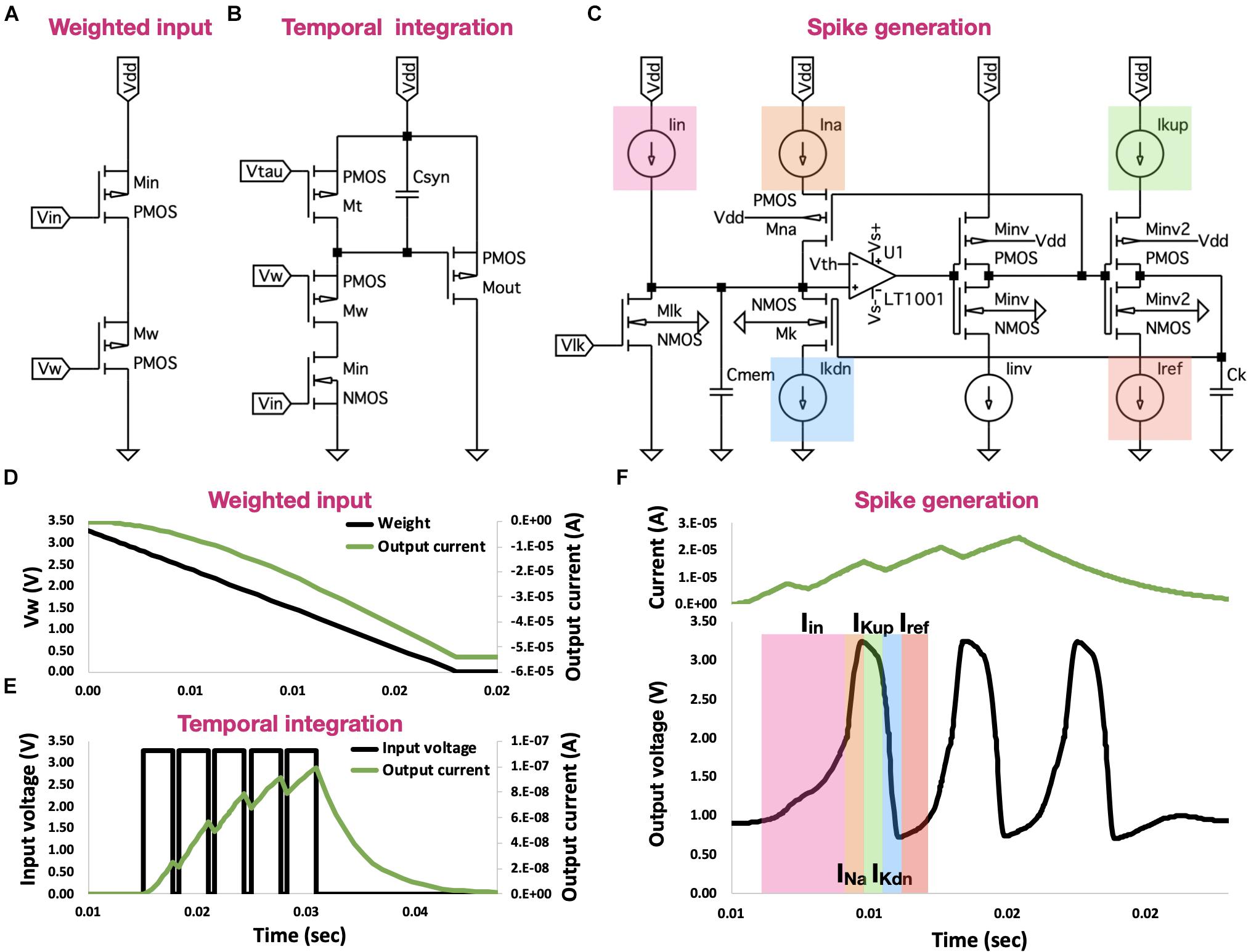
Figure 1. Neuron building blocks. (A) Pulse current source synapse. This voltage-controlled current source is activated by an active-low input spike, producing a current, which follows the input voltage pattern and dynamic. (B) Subthreshold first-order LPF circuit. This circuit provides temporal control of both charging and discharging of a capacitor, allowing for temporal integration of incoming spikes. (C) Voltage-amplifier LIF neuron. This spike generating circuit provides precise control of the generated spikes, including spikes’ rise time, width, fall time, and refractory period. (D) Signal traces for the current-source synapse. When spike arrives (synapse is activated-low; Vin), current Isyn is proportionally generated. This synapse offers magnitude control where Isyn is proportionally correlated to Vw. (E) Signal traces for the log-domain integrator synapse. Log-domain integrator synapse features a linear integration of incoming spikes, where ahead of saturation, each spike equally contributes to Isyn. (F) Signal traces for the voltage-amplifier LIF neuron. Neuron is driven by Iin, which was generated by the subthreshold first-order LPF circuit (described earlier). Circuit has two voltage inverters: first inverter Iinv1 drives current INA, and second inverter Iinv2 drives the IK currents. These currents adhere to the behavior of biological neurons, providing precise control of spikes’ dynamic.
The pulse current-source synapse (Figure 1A), proposed by Mead (1989), was one of the first artificial synapse circuits created. It is a voltage-controlled current source, which is driven by an active-low input spike. The resulting current Isyn is defined using:
Where Vdd is the supply voltage, Io is the leakage current of the transistor Mw, which is activated in the subthreshold regime, κ is the subthreshold slope factor and UT is a thermal voltage (at room temperature, it is approximately 26 mV). This circuit allows for controlling the magnitude of Isyn such that when Vw equals Vdd, Isyn is I0. As we decrease Vw, I0 is scaled up exponentially, increasing Isyn accordingly (Figure 1D). While offering control over Isyn’s magnitude, the pulse current-source synapse does not provide temporal modulation.
The subthreshold first-order LPF circuit (Figure 1B), proposed by Merolla and Boahen (2004), offers linear integration of incoming spikes. This circuit is built upon the charge and discharge synapse [described in Bartolozzi and Indiveri (2007)], which provides temporal control of charging and discharging of Csyn. In the charge and discharge synapses, the incoming active-high spikes activate the transistor Min. During a spike, Vsyn decreases linearly, at a rate set by the net current Iw−Iτ, where Iw is the current driven through transistor Mw (and regulated by Vw) and Iτ is the current driven through transistor Mτ (and regulated by Vτ). This net current is responsible for discharging Csyn. The linearly decreasing Vsyn drives Isyn by regulating transistor Mout. In this log-domain circuit, the logarithmic relationship between the transistor’s Vgs and its current is used to exhibit overall linear properties [see (Indiveri et al., 2011) for a detailed analysis]. The governing equations of this synapse during a spike and between spikes are:
where and ti are the times at which spike i arrives and terminates, respectively, and Isyn are the Isyn in times and ti, respectively, τc is the time constant for the capacitor charge, which equals UT = C/κ(Iw−Iτ), and τd is the time constant for the capacitor-discharge, which equals UT = C/κIτ. Controlling the charge and discharge of Csyn allows for temporal control of both rise and fall times of Vsyn, thus providing the ability to temporally integrate multiple incoming spikes (Figure 2E).
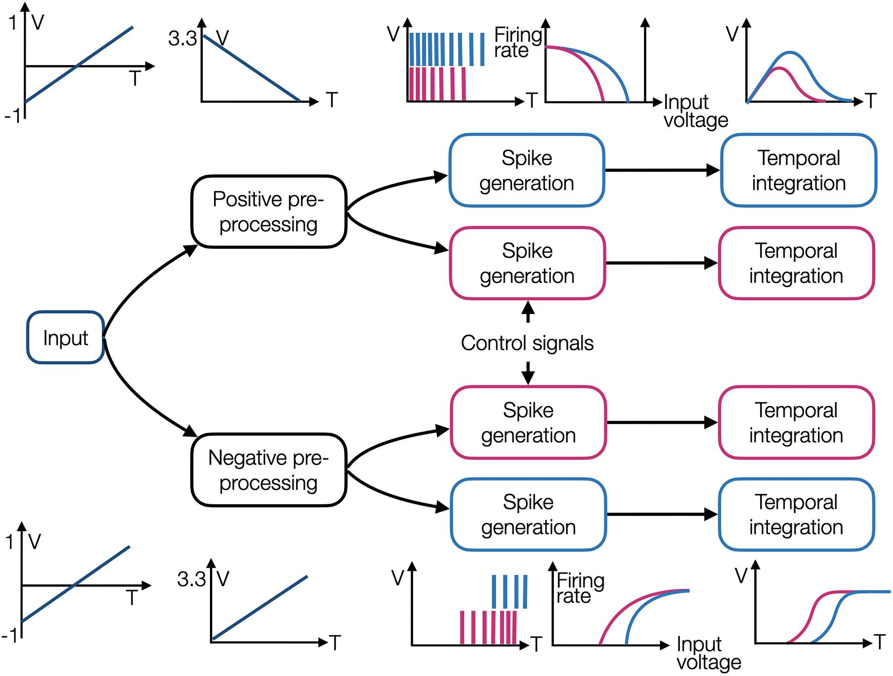
Figure 2. An illustration of four OZ neurons grouped into two branches, one with positive and the other with negative encoders. Each branch initiates with an input preprocessing module, and each neuron comprises a spike generation and temporal integration modules. Each neuron has different tuning, and it is therefore producing spikes in a different dynamic.
The voltage-amplifier LIF neuron is a spike generating circuit proposed by van Schaik (2001) and Figure 1C. This circuit enhances the classic axon-hillock neuron design [described in Mead (1989)] with precise control of the generated spikes’ dynamic, including spikes’ rise time, width, fall time, and refractory period. Capacitor Cmem models the neuron membrane and Vlk, which regulates the conductance of transistor Mlk, controls its leakage current Ilk. In the absence of an input current from incoming spikes (flat phase), Ilk drives the membrane voltage Vmem down to 0 V. When an input current is apparent, the net incoming current Iin−Ilk is charging Cmem, increasing Vmem. When Vmem exceeds Vth, an action potential is generated via an operational amplifier (op-amp). This action potential is introduced into a voltage inverter, where high logical states are transformed into low logical states and vice versa. A low logical voltage state activates transistor MNa, through which INa current is driven, charging Cmem and creating a sustained high voltage (constituting the spike). A second voltage inverter drives Ikup through transistor Minv2, charging Ck, thus controlling spike’s width. As Ck is charging, it activates transistor Mk, through which Ik is driven. Ik discharges Cmem and when Vmem drops below Vth, the amplifier’s output drops to a low state. In response, the first voltage inverter’s output is driven high, deactivating transistor MNa, thus terminating INa. The second inverter’s output voltage is driven low, terminating Ikup and allowing Iref to discharge Ck. As long as Iref is not strong enough to discharge Ck, the circuit cannot be further stimulated by incoming current (assuming Iin < Ik), constituting a refractory period. The generated spikes are shown in Figure 1F. This process is a direct embodiment of the biological behavior, in which an influx of sodium ions (Na+) and a delayed outflux of potassium ions (K+) govern the initiation of an action potential.
Results
Circuit Design
In our circuit design, stimulus x is introduced through preprocessing modules to two branches, one connected to positively encoded OZ neurons and the other to negatively encoded OZ neurons. These preprocessing modules accept an input voltage ranging from −1 to 1 V (corresponding to the default input normalization scheme taken by NEF) and produce an output voltage ranging from 0 to 3.3 V. Each OZ neuron is comprised of two consecutive modules: a spike generator and a temporal integrator. Each spike generator is characterized by a tuning curve, modulated using control signals, thus realizing Eq. 1. A generated spike train is introduced to a temporal integrator, which integrates the incoming spikes, thus realizing Eq. 2 and constituting a NEF-inspired neuron. The circuit schematic for two negatively encoded and two positively encoded neurons is shown in Figure 2. The negative preprocessing circuit comprises two consecutive modules: the first one inverses the voltage and aligns it to initiate at 0 V, and the second reinverts and scales it so it will terminate at 3.3 V (circuit’sVdd) (Figure 3A). The first module uses an op-amp based adder to add 1 V to the input signal (aligning it to 0 V) and inverts it according to Vo = −(VV−), where V and V− are the op-amp’s input terminals. The resulted voltage is ranging from 0 to 2 V. The second module uses an inverter amplifier that scales its input voltage according to −Rfb/Rin, where Rfb is the feedback resistor and Rin is the amplifier’s input terminal resistor. Here, Rfb2 = 1.65kOhm and Rin2 = 1kOhm, achieving a scaling factor of −1.65, which transform 2 to 3.3 V output. The positive preprocessing module resembles the negative preprocessing module, with the addition of another voltage inverter, which produces a similar waveform, initiating at 3.3 V and terminating at 0 V.
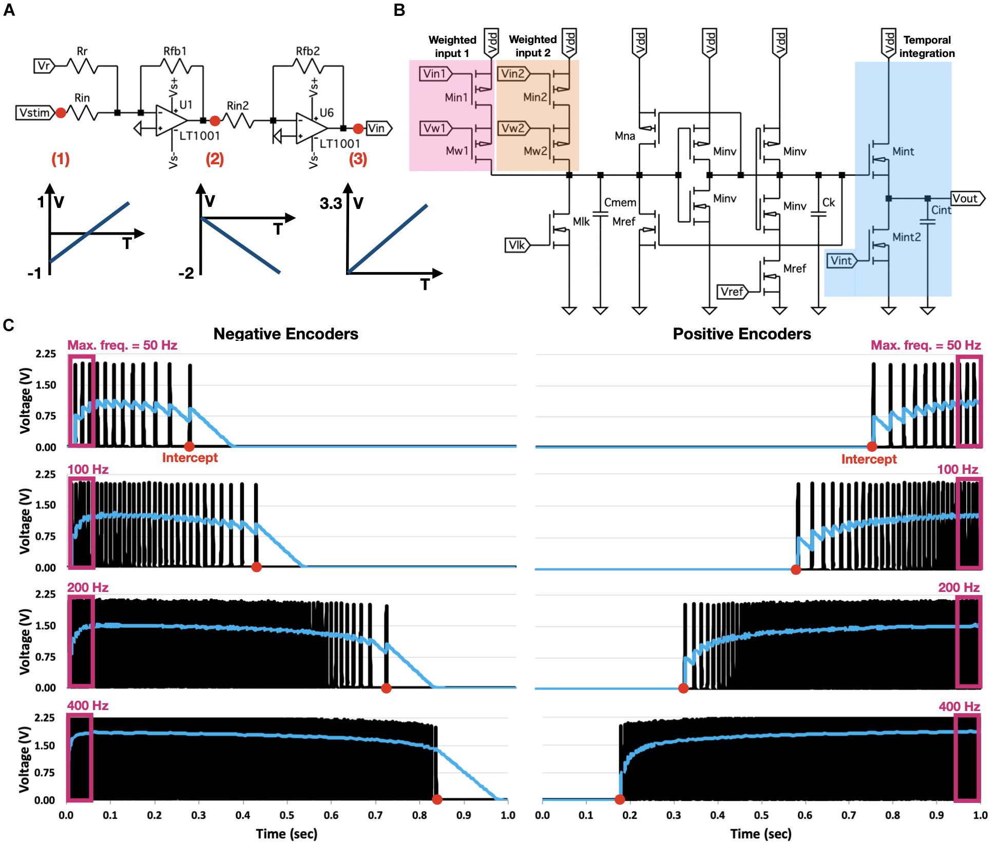
Figure 3. OZ neuron analog design. (A) Preprocessing module for negatively encoded OZ neurons. Module inverses input voltage, aligns it to initiate at 0 V, and reinverts and scales it to terminate at 3.3 V. (B) Neuron’s spike generator. Voltages from two weighted inputs are transformed into a proportional current, injected into a modified voltage-amplifier LIF neuron. Neuron produces a spike train according to its response dynamic. Spike train is introduced into a temporal integration circuit. (C) Eight OZ neurons, four of them are positively encoded (right), and four are negatively encoded (left). All neurons were stimulated with a linearly increasing voltage, rising from –1 to 1 V. Each neuron was modulated with various values of Vlk to produce a spike train at a particular rate, starting from a specific input (intercept).
The OZ neuron is shown in Figure 3B. It is based on modified versions of the pulse current source synaptic circuit (for weighted input), the voltage-amplifier LIF neuron (for spike generation), and the subthreshold first-order LPF circuit (for temporal integration). The pulse-current source synapse is used to convert an input voltage to a proportional current, introduced into the spike generation circuit, and defined by Vw according to Eq. 3. The voltage-amplifier LIF neuron’s response dynamic is predominantly determined by the values of Ikup, Ikdn, INa, and Iref and the leakage current Ilk (driven through transistor Mlk), which are regulated, respectively, by of Vkup, Vkdn, VNa, Vref, and Vlk via dedicated transistors. Therefore, this neuron has five degrees of freedom (DOF): Vlk controls the discharge rate of Cmem, Vref controls spikes’ refractory period, Vkup and Vkdn control the fall time of the generated spikes, and VNa controls the spikes’ rise time. Furthermore, its spiking dynamic relies on an op-amp, which is comprised of multiple transistors and resistors. OZ’s spike generator is a NEF-optimized circuit design, where Vup, VNa, and Vkdn are redundant. Furthermore, it does not rely on op-amp for spike generation, as the amplifier has no significant functional effect in terms of neuron’s firing rate and intercept (see section “Discussion”). A NEF-tailored design should also enable high-dimensional input representation, which can be achieved by concatenating the input module (highlighted in Figure 3B as weighted input; see section “Circuit Analysis”). Finally, temporal integration can be achieved via a simplified LPF temporal integration circuit. In OZ, capacitor Cint is charged by current Iint, which is activated by the generated spike train and driven through transistor Mint. Cint is discharging at a constant rate through a leakage current, which is driven through transistor Mint2 and regulated by a continuously held voltage Vint. The voltage on Cint constitutes the OZ neuron’s output.
A useful way of representing a neuron’s response to varying inputs is by using a response, or a tuning curve, which is one of the most fundamental concepts of NEF. In NEF, a tuning curve is defined using an intercept, the value for which the neuron starts to produce spikes at a high rate, and its maximal firing rate. OZ’s tuning curve can be programmed to control both. For circuit analysis, we built eight OZ neurons, four with positive and four with negative encoders. Each neuron has d+2 DOF, where d is the dimensionality of the input, corresponding to d values of Vw, which regulate each input dimension, and Vlk and Vref correspond to the two other DOF. To demonstrate OZ, we built eight neurons; each was defined to feature a different intercept and maximal firing rate. Each neuron was stimulated with the same input voltage, which linearly increased from −1 to 1 V over 1 s. Results are shown in Figure 3C.
Circuit Analysis
Architectural Design
For the sake of discussion, we will consider one-dimensional (1D) OZ neurons. First, we shall consider the classic voltage-amplifier LIF neuron, shown in Figure 1C. This design relies on an op-amp for spike generation. From a functional perspective, the op-amp provides the neuron with a digital attribute, splitting the neuron into an analog pre-op-amp circuit and a digital post-op-amp circuit. Particularly, when an incoming current is inducing Vmem to exceed a predefined threshold voltage, the op-amp yields a square signal, which generates a sharp INa response. This fast response induces sharp swing-ups in Vmem and Vout. Without the op-amp, this transition between states is gradual (Figures 4A–C). Although both designs permit spike generation, the op-amp-based design can generate spikes in a higher frequency and amplitude. To compensate for that, we can discard both INa and Ikup controls through the removal of their regulating transistors. Removing these resistance-inducing transistors maximizes INa and Ikup, thus achieving op-amp-like frequency and amplitude (Figures 4D–F). Moreover, without the op-amp, there is no need to explicitly define a threshold, providing a more straightforward and biologically plausible design.
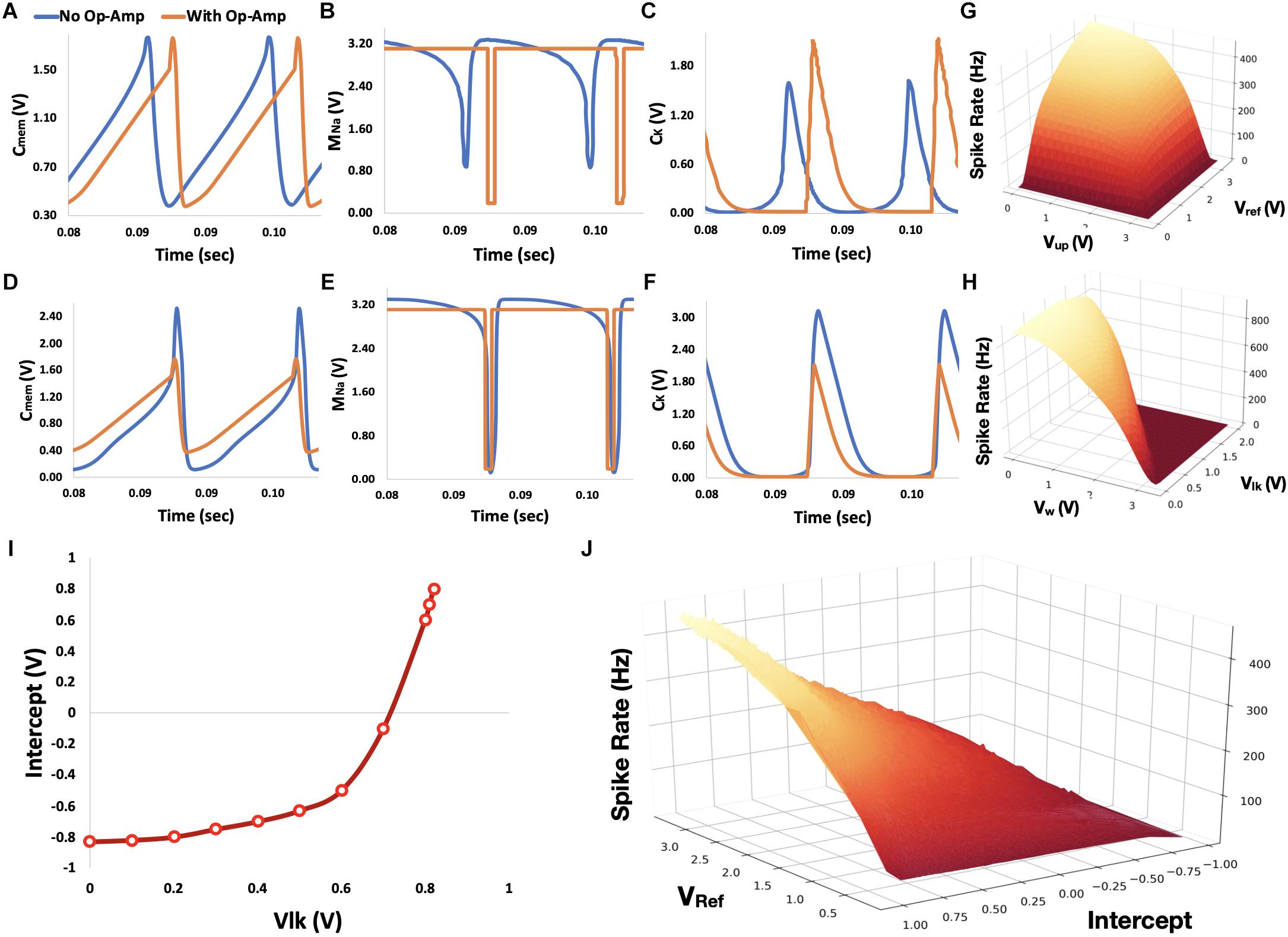
Figure 4. Circuit analysis. (A–C) Voltage traces for the subthreshold first-order LPF neuron circuit with and without op-amp for spike generation (colored orange and blue, respectively). Traces for the voltages over Cmem, gate of MNa, and CK are shown in panels A–C, respectively. (D–F) Similar traced to panels A–C, where the transistor-based controls of INa and Ikup were eliminated. (G) Neuron’s spike rate as a function of Vref and Vup. (H) Neuron’s spike rate as a function of Vw and Vlk(I) Neuron’s intercept as a function of Vlk. (J) For a given intercept (determined by Vlk), a neuron’s spiking rate can be determined by Vref. Vw was held constant at 2.4 V for both I and J panels.
Neuron Control
Did we lose control over the maximal firing rate over our neuron by eliminating the regulation of Ikup? Fortunately, both Ikup and Iref impact neuron’s firing rate. Although Ikup limits neuron’s firing rate by governing the rise time of the generated spikes, Iref does that by setting the refractory period between spikes. Controlling both currents is redundant as both imply similar constraints, as shown in Figure 4G (Vlk and Vw are held constant at 2.2 and 0.5 V, respectively).
Vlk controls the discharge rate of Cmem by regulating a leakage current through transistor Mlk. As long as this leakage current is lower than the input current (driven through the weighted input module), Vmem will rise toward saturation. As we decrease Vlk, leakage current drops and Cmem charged faster. As a result, the neuron’s intercept (the input value for which the neuron’s initiate spikes at a high rate) increases for positively encoded neurons and decreases for negatively encoded neurons. Neurons exhibit maximal firing rate when their input voltage is either −1 or 1 V, depending on the neuron’s encodings. The maximal firing rate is proportionally dependent on the charging status of membrane capacitance Cmem. The faster Cmem is charging, the more frequent the neuron will emit spikes. However, a neuron’s maximal firing rate is not entirely decoupled from its intercept. Although a neuron’s intercept is controlled by Vlk, it can also be modulated by Vw, which provides a magnitude control for the input current. Therefore, although Vlk can be used to define the neuron’s intercept, Vw can impose on it a firing rate constraint. For example, the neuron’s spiking rate will not exceed 400 Hz, when Vw is set to 2.2 V. Vlk and Vw imposed constraint on neuron’s spiking rate is demonstrated in Figure 4H (Vref and Vup are held constant at 3.3 and 1 V, respectively).
Figures 4I,J summarizes the control of the neuron’s intercept and spiking rate using Vref and Vlk (whereas Vw was held constant at 2.4V). Through curve and surface fittings (R2 > 0.98), neuron’s intercept Nint can be described with:
and neuron’s maximal firing rate NFR with:
In Figure 5, the tuning curves of our eight OZ neurons, along with the tuning curves of eight simulated neurons, which were computed directly with NEF, are demonstrated. The tuning curves indicate varying intercepts and spiking rates, showcasing the produced spike trains’ high predictability and the full correspondence between our hardware design and NEF. In Figures 5B,D, we compared 2D tuning curves. It was achieved with OZ by concatenating two weighted inputs: x1 and x2, weighting them with Vw1 and Vw2, respectively. Results show the high predictability of the neuron in response to a high-dimensional stimulus.
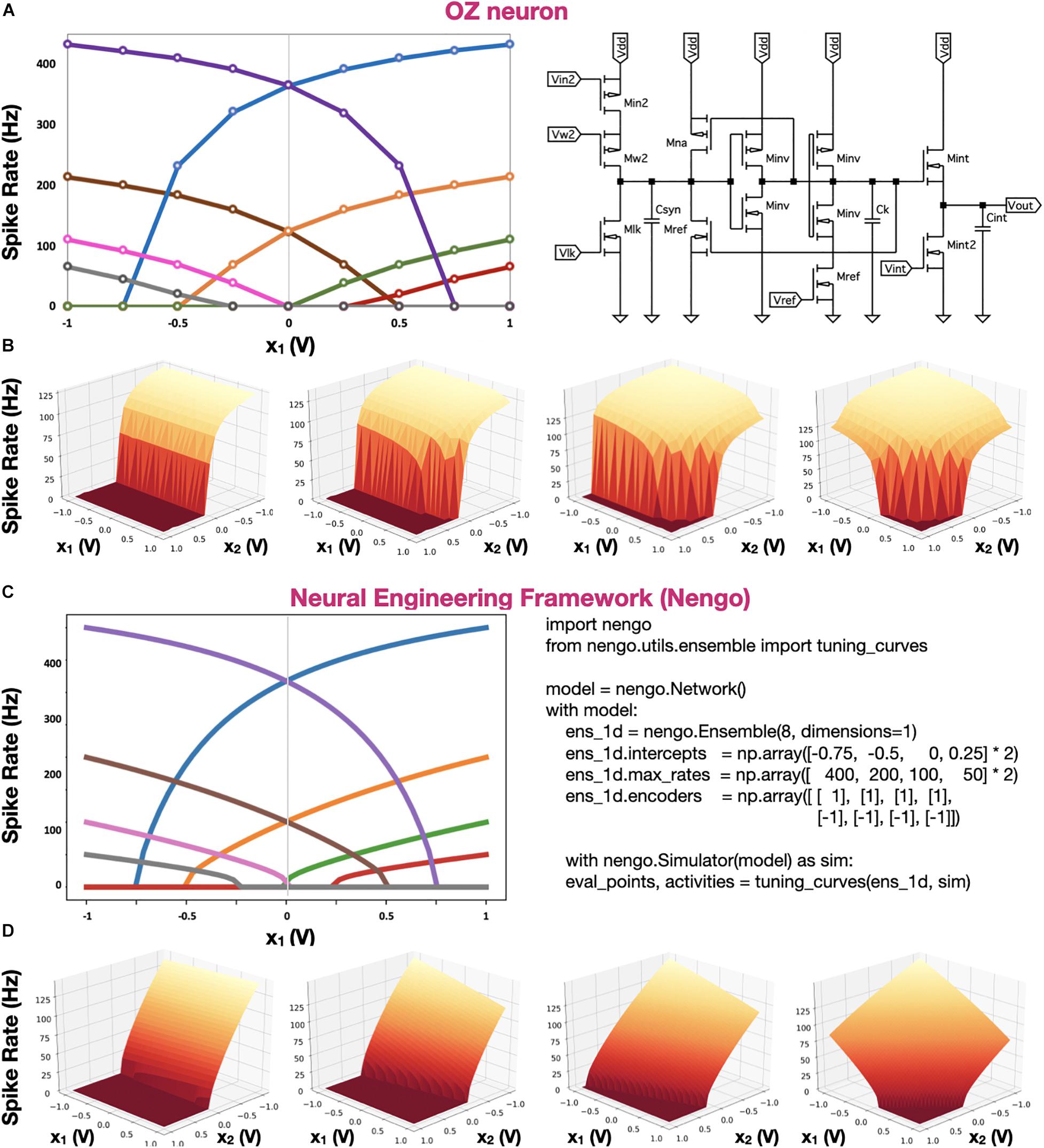
Figure 5. OZ and Nengo neuron tuning curves. (A) Tuning curves of eight 1D hardware-based OZ neurons. (B) Tuning curves of four 2D hardware-based OZ neurons. (C) Tuning curves of eight NEF-based simulated neurons, directly computed with Nengo. (D) Four tunning curves of four 2D simulated neurons (D). In panels A,C, each color stands for one neuron spiking at a specific rate in response to an input voltage (x1). In OZ-based 2D representation, Vw for x1 was held constant at 2.5 V, Vref at 0.4 V, and Vlk at 0.729. Vw values for x2 were 3.3, 2.8, 2.6, and 2.4 V, left to right, respectively.
Discussion
Numerous digital and analog designs of spiking neurons have been previously proposed. For example, Yang et al. (2018b) proposed a biologically plausible, conductance-based implementation of spiking neurons with an FPGA. This design was used to simulate 1 million neurons by utilizing six state-of-the-art FPGA chips simultaneously, achieving biological plausibility and scale (Yang et al., 2018a). Furthermore, it was shown to feature multicompartmental neuron design, supporting the morphologically detailed realization of neural networks (Yang et al., 2019). Biologically plausible spiking neurons were also implemented in analog circuits, featuring spike adaptation (Aamir et al., 2017). Although incredibly versatile and highly configurable, these designs were guided by a bottom–up approach, tailored to reproduce biological behavior. However, to achieve function-optimized neural networks (e.g., for neurorobotics or other smart-edge devices), top–bottom modeling is more suitable (Eliasmith and Trujillo, 2014). By throwing out morphological and physiological constraints, the NEF allows top–down optimization, with which high-level specification can be realized in spiking neurons with a minimal number of explicitly defined neuronal characteristics.
NEF is one of the most utilized theoretical frameworks in neuromorphic computing. A version of NEF was compiled on various neuromorphic digital systems, such as Intel’s Loihi and IBM’s TrueNorth (Fischl et al., 2018; Lin et al., 2018), as well as on hybrid analog/digital systems such as the NeuroGrid (Boahen, 2017). NEF-inspired neurons were directly implemented in both digital (Wang et al., 2017) and analog (Indiveri et al., 2011) circuitry. Although digital NEF-inspired implementations are versatile and programmable, they are fundamentally less energy-efficient and footprint-restricted in comparison with analog circuitry (Amara et al., 2006). Current analog implementations of NEF-inspired neurons rely on the inherent stochasticity in the fabrication process of integrated circuits to create the variational neurons’ tuning required to span a representation space (Mayr et al., 2014; Boahen, 2017) or to support machine learning (Tripathi et al., 2019).
Neurons in NEF represent mathematical constructs, and their accuracy of that representation is fundamentally limited to the neurons’ tuning curves. A tunning curve is defined using an intercept and maximal spike rate. Intercepts represent the part of the representation space for which the neuron will fire. In 1D, uniformly distributed intercepts will uniformly span the representation space. A neuron with an intercept of 0 will be active for 50% of that space, and a neuron with an intercept of 0.75 will be active for only 7.5% of that space. However, using randomly distributed tuning curves would require many more neurons to achieve adequate space spanning. When an input does not invoke a neuron to spike, that neuron is essentially a waste of space and energy.
Moreover, as we advance toward representing values in higher dimensions, articulating and carefully defining neurons’ tuning curves become a critical design factor. This design factor was attested by the authors of Mayr et al. (2014), as they discussed their analog implementation of a NEF-inspired neuron: “as the spread of the curves is determined by random effects of the manufacturing process, individual instances of the ADC [the designated application for that design] have to be checked for sufficient spread, thus defining a yield in terms of ADC resolution. When comparing the two families of tuning curves, the main observation is that the Nengo generated neurons tend to vary more, especially in their gain… this has a significant impact on the overall computation. If the neurons do not encode for sufficiently different features of the input signal, the representation of the input signal degrades” (Mayr et al., 2014).
Moreover, our proposed implementation offers a high-dimensional representation. Distributing intercepts uniformly between −1 and 1 makes sense for 1D ensembles. Because a neuron’s intercept defines the part of the representation space in which this neuron is firing, in 1D representation, uniformly distributed intercepts create a uniform spanning of that space. In higher dimensions, the proportions of activity are getting smaller (or larger for negatively encoded neurons). In high dimensions, the naive distribution of intercepts results in many neurons, either rarely producing spikes or always active (Figure 6A). In both cases, these neurons are essentially not contributing to the representation. A representation space in 2D is a 3D sphere, in which each neuron’s encoder points to a cap, which specifies the space in which that neuron is active (Gosmann and Eliasmith, 2016). The intercept is the location of the cap’s cutoff plane. The ratio between the cap’s and the sphere’s volumes is the percentage of the representation space in which a neuron is active. A generalized sphere in a higher dimension is a hyper-sphere. The volume of a hyper-sphere cap vcap is defined with:
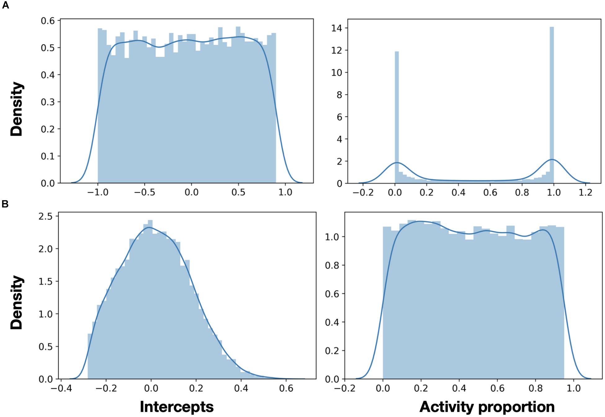
Figure 6. Neurons activity in high dimension. (A) In 32D representation, a uniform distribution of intercepts (left) creates many neurons, which are either always or never active (right). (B) Using a rational distribution of intercepts (using Eq. 7), a uniform activity pattern of neurons across the representation space can be generated.
where Cd is the volume of a unit hypersphere of dimension d and radius r, h is the cap’s height, and Ix(a,b) is the regularized incomplete beta function. Here, r = 1 (representation is in [−1,1]), and h = x−1, where x is the intercept. The ratio p between the hypersphere’s volume Cd and its cap’s volume vcap is:
To more efficiently span in high-dimensional representation space, we can use the inverse of Eq. 6 to derive a desired p value, the intercept, which will create it. This equation is defined with:
With Eq. 7, we can generate the intersects to better span the representation space. Utilizing this equation can provide the intersects distribution for which the spikes activity pattern is uniform (Figure 6B). This is a clear example of the importance of being able to modulate neuron’s tuning curves in high-dimensional representation. The importance of the discussion earlier was recently highlighted in DeWolf et al. (2020) in the context of neuro-robotics.
Here, we presented the OZ neuron—a programmable analog implementation of a spiking neuron, which can have its tuning curve explicitly defined. With our system design, for a uniform distribution of tuning curves (required in most low-dimensional applications), only one among the positive and negative branches has to be defined, cutting in half the number of neurons, which have to be controlled. Because we can design the neurons’ tuning curve to accurately span the representation space following a particular application’s needs, the required number of neurons for spanning that space can be significantly reduced. Moreover, uniquely, neurons’ tuning curves can be changed in real-time to provide dynamically modulated neuromorphic representation. However, when the required number of neurons is large, the apparent overhead of control must be considered. Our design can be scaled to a full very large-scale integration neuromorphic circuit design, providing analog, distributed, and energy-efficient neuromorphic representation of high-dimensional mathematical constructs.
Data Availability Statement
Model simulation will be provided upon request.
Author Contributions
AH designed the circuits and performed circuit simulation and analysis. EE conceptualized the research, designed the circuits, and wrote the manuscript. Both authors contributed to the article and approved the submitted version.
Funding
This research was supported by the Israel Innovation Authority (EzerTech) and the Open University of Israel research grant.
Conflict of Interest
The authors declare that the research was conducted in the absence of any commercial or financial relationships that could be construed as a potential conflict of interest.
Acknowledgments
The authors would like to thank Tamara Perelman Tsur for her insightful comments.
References
Aamir, S. A., Muller, P., Kriener, L., Kiene, G., Schemmel, J., and Meier, K. (2017). “From LIF to AdEx neuron models: accelerated analog 65 nm CMOS implementation,” in Proceedings of the IEEE Biomedical Circuits and Systems Conference (BioCAS), Turin. doi: 10.1109/BIOCAS.2017.8325167
Amara, A., Amiel, F., and Ea, T. (2006). FPGA vs. ASIC for low power applications. Microelectron. J. 37, 669–677. doi: 10.1016/j.mejo.2005.11.003
Analog Devices (2008). LTspice simulator. Available online at: http://www.analog.com/en/design-center/design-tools-and-calculators/ltspice-simulator.html (accessed September 26, 2020).
Ankri, L., Ezra-Tsur, E., Maimon, S. R., Kaushansky, N., and Rivlin-Etzion, M. (2020). Antagonistic center-surround mechanisms for direction selectivity in the retina. Cell Rep. 31:107608. doi: 10.1016/j.celrep.2020.107608
Bartolozzi, C., and Indiveri, G. (2007). Synaptic dynamics in analog VLSI. Neural Comput. 19, 2581–2603. doi: 10.1162/neco.2007.19.10.2581
Bekolay, T., Bergstra, J., Hunsberger, E., DeWolf, T., Stewart, T., Rasmussen, D., et al. (2014). Nengo: a Python tool for building large-scale functional brain models. Front. Neuroinform. 7:48. doi: 10.3389/fninf.2013.00048
Benjamin, B. V., Gao, P., McQuinn, E., Choudhary, S., Chandrasekaran, A., Bussat, J.-M., et al. (2014). Neurogrid: a mixed-analog-digital multichip system for large-scale neural simulations. Proc. IEEE 102, 699–716. doi: 10.1109/JPROC.2014.2313565
Boahen, K. (2017). A neuromorph’s prospectus. Comput. Sci. Eng. 19, 14–28. doi: 10.1109/MCSE.2017.33
Burkitt, A. (2006). A review of the integrate-and-fire neuron model: I. Homogeneous synaptic input. Biol. Cybern. 95, 1–19. doi: 10.1007/s00422-006-0068-6
Davies, M., Srinivasa, N., Lin, T.-H., Chinya, G., Cao, Y., Choday, S. H., et al. (2018). Loihi: a neuromorphic manycore processor with on-chip learning. IEEE Micro 38, 82–99. doi: 10.1109/MM.2018.112130359
DeBole, M. V., Taba, B., Amir, A., Akopyan, F., Andreopoulos, A., Risk, W. P., et al. (2019). TrueNorth: accelerating from zero to 64 million neurons in 10 years. Computer 52, 20–29. doi: 10.1109/MC.2019.2903009
DeWolf, T., Jaworski, P., and Eliasmith, C. (2020). Nengo and low-power AI hardware for robust, embedded neurorobotics. arXiv [Preprint]. arXiv: 2007.10227 doi: 10.3389/fnbot.2020.568359
Eliasmith, C., and Anderson, C. H. (2003). Neural engineering: Computation, Representation, and Dynamics in Neurobiological Systems. Cambridge, MA: MIT press.
Eliasmith, C., Stewart, T. C., Choo, X., Bekolay, T., DeWolf, T., Tang, Y., et al. (2012). A large-scale model of the functioning brain. Science 338, 1202–1205. doi: 10.1126/science.1225266
Eliasmith, C., and Trujillo, O. (2014). The use and abuse of large-scale brain models. Curr. Opin. Neurobiol. 25, 1–6. doi: 10.1016/j.conb.2013.09.009
Fischl, K., Andreou, A., Stewart, T., and Fair, K. (2018). “Implementation of the neural engineering framework on the TrueNorth neurosynaptic system,” in Proceedings of the IEEE Biomedical Circuits and Systems Conference (BioCAS), Cleveland, OH. doi: 10.1109/BIOCAS.2018.8584720
Furber, S., Galluppi, F., Temple, S., and Plana, L. A. (2014). The spinnaker project. Proc. IEEE 102, 652–665. doi: 10.1109/JPROC.2014.2304638
Gosmann, J., and Eliasmith, C. (2016). Optimizing semantic pointer representations for symbol-likeprocessing in spiking neural networks. PloS One 11:e0149928. doi: 10.1371/journal.pone.0149928.g006
Indiveri, G., and Douglas, R. (2000). Neuromorphic vision sensors. Science 288, 1189–1190. doi: 10.1126/science.288.5469.1189
Indiveri, G., Linares-Barranco, B., Hamilton, T. J., van Schaik, A., Etienne-Cummings, R., Delbruck, T., et al. (2011). Neuromorphic silicon neuron circuits. Front. Neurosci. 5:73. doi: 10.3389/fnins.2011.00073
Krestinskaya, O., James, A. P., and Chua, L. (2019). Neuromemristive circuits for edge computing: a review. IEEE Trans. Neural Netw. Learn. Syst. 31, 4–23. doi: 10.1109/TNNLS.2019.2899262
Krichmar, J. L., and Wagatsuma, H. (2011). Neuromorphic and Brain-Based Robots. Cambridge: Cambridge University Press. doi: 10.1017/CBO9780511994838
Lin, C.-K., Wild, A., Chinya, G., Cao, Y., Davies, M., Lavery, D. M., et al. (2018). Programming spiking neural networks on intel’s loihi. Computer 51, 52–61. doi: 10.1109/MC.2018.157113521
Liu, S.-C., and Delbruck, T. (2010). Neuromorphic sensory systems. Curr. Opin. Neurobiol. 20, 288–295. doi: 10.1016/j.conb.2010.03.007
Liu, S.-C., Delbruck, T., Indiveri, G., Whatley, A., and Douglas, R. (2014). Event-Based Neuromorphic Systems. Hoboken, NJ: John Wiley & Sons. doi: 10.1002/9781118927601
Mayr, C., Partzsch, J., Noack, M., and Schuffny, R. (2014). Configurable analog-digital conversion using the neural engineering framework. Front. Neurosci. 8:201. doi: 10.3389/fnins.2014.00201
Merolla, P., and Boahen, K. (2004). “A recurrent model of orientation maps with simple and complex cells,” in Proceedings of the Advances in Neural Information Processing Systems 16, eds S. Thrun and L. Saul (Cambridge, MA: MIT Press), 995–1002.
Mundy, A., Knight, J. S. T., and Furber, S. (2015). “An efficient SpiNNaker implementation of the neural engineering framework,” in Proceedings of the International Joint Conference on Neural Networks (IJCNN), Killarney. doi: 10.1109/IJCNN.2015.7280390
Nagel, L., and Pederson, D. (1973). SPICE (Simulation Program With Integrated Circuit Emphasis) Technical Report No. UCB/ERL M382 April 1973. Berkeley, CA: University of California.
Nichols, K., Kazmierski, T., Zwolinski, M., and Brown, A. (1994). Overview of SPICE-like circuit simulation algorithms. IEE Proc. Circuits Devices Syst. 141, 242–250. doi: 10.1049/ip-cds:19941246
Stewart, T., and Eliasmith, C. (2014). Large-scale synthesis of functional spiking neural circuits. Proc. IEEE 102, 881–898. doi: 10.1109/JPROC.2014.2306061
Tripathi, A., Arabizadeh, M., Khandelwal, S., and Thakur, C. S. (2019). “Analog Neuromorphic System Based on Multi Input Floating Gate MOS Neuron Model,” in Proceedings of the IEEE International Symposium on Circuits and Systems (ISCAS), Sapporo. doi: 10.1109/ISCAS.2019.8702492
Tsur, E. E., and Rivlin-Etzion, M. (2020). Neuromorphic implementation of motion detection using oscillation interference. Neurocomputing 374, 54–63. doi: 10.1016/j.neucom.2019.09.072
van Schaik, A. (2001). Building blocks for electronic spiking neural networks. Neural Netw. 6, 617–628. doi: 10.1016/S0893-6080(01)00067-3
Wang, R., Thakur, C. S., Cohen, G., Hamilton, T. J., Tapson, J., and van Schaik, A. (2017). Neuromorphic hardware architecture using the neural engineering framework for pattern recognition. IEEE Trans. Biomed. Circuits Syst. 11, 574–584. doi: 10.1109/TBCAS.2017.2666883
Yang, S., Deng, B., Wang, J., Li, H., Lu, M., Che, Y., et al. (2019). Scalable digital neuromorphic architecture for large-scale biophysically meaningful neural network with multi-compartment neurons. IEEE Trans. Neural Netw. Learn. Syst. 31, 148–162. doi: 10.1109/TNNLS.2019.2899936
Yang, S., Wang, J., Deng, B., Liu, C., Li, H., Fietkiewicz, C., et al. (2018a). Real-time neuromorphic system for large-scale conductance-based spiking neural networks. IEEE Trans. Cybern. 49, 2490–2503. doi: 10.1109/TCYB.2018.2823730
Yang, S., Wang, J., Lin, Q., Deng, B., Wei, X., Liu, C., et al. (2018b). Cost-efficient FPGA implementation of a biologically plausible dopamine neural network and its application. Neurocomputing 314, 394–408. doi: 10.1016/j.neucom.2018.07.006
Zaidel, Y., Shalumov, A., Volinski, A., Supic, L., and Ezra Tsur, E. (2021). Neuromorphic NEF-based inverse kinematics and PID control. Front. Neurorobot. 15:631159. doi: 10.3389/fnbot.2021.631159
Keywords: neural engineering framework, spiking neural networks, neuromorphic electronics, neuromorphic engineering, brain-inspired electronics
Citation: Hazan A and Ezra Tsur E (2021) Neuromorphic Analog Implementation of Neural Engineering Framework-Inspired Spiking Neuron for High-Dimensional Representation. Front. Neurosci. 15:627221. doi: 10.3389/fnins.2021.627221
Received: 08 November 2020; Accepted: 25 January 2021;
Published: 22 February 2021.
Edited by:
Jonathan Mapelli, University of Modena and Reggio Emilia, ItalyReviewed by:
Shuangming Yang, Tianjin University, ChinaQinru Qiu, Syracuse University, United States
Copyright © 2021 Hazan and Ezra Tsur. This is an open-access article distributed under the terms of the Creative Commons Attribution License (CC BY). The use, distribution or reproduction in other forums is permitted, provided the original author(s) and the copyright owner(s) are credited and that the original publication in this journal is cited, in accordance with accepted academic practice. No use, distribution or reproduction is permitted which does not comply with these terms.
*Correspondence: Elishai Ezra Tsur, ZWxpc2hhaUBOQkVMLWxhYi5jb20=