Backpropagation With Sparsity Regularization for Spiking Neural Network Learning

The spiking neural network (SNN) is a possible pathway for low-power and energy-efficient processing and computing exploiting spiking-driven and sparsity features of biological systems. This article proposes a sparsity-driven SNN learning algorithm, namely backpropagation with sparsity regularization (BPSR), aiming to achieve improved spiking and synaptic sparsity. Backpropagation incorporating spiking regularization is utilized to minimize the spiking firing rate with guaranteed accuracy. Backpropagation realizes the temporal information capture and extends to the spiking recurrent layer to support brain-like structure learning. The rewiring mechanism with synaptic regularization is suggested to further mitigate the redundancy of the network structure. Rewiring based on weight and gradient regulates the pruning and growth of synapses. Experimental results demonstrate that the network learned by BPSR has synaptic sparsity and is highly similar to the biological system. It not only balances the accuracy and firing rate, but also facilitates SNN learning by suppressing the information redundancy. We evaluate the proposed BPSR on the visual dataset MNIST, N-MNIST, and CIFAR10, and further test it on the sensor dataset MIT-BIH and gas sensor. Results bespeak that our algorithm achieves comparable or superior accuracy compared to related works, with sparse spikes and synapses.

1. Introduction

Artificial intelligence (AI) has shown impressive abilities in various tasks such as computer vision, natural language processing, and decision making. For example, AlphaGo Zero defeated the world champion of the game of Go (Silver et al., 2017). However, the power consumption of AlphaGo Zero is about 1kW (Frenkel et al., 2021), which is 50× higher than the 20W power budget of the human brain (Roy et al., 2019). The brain-inspired spiking neural network (SNN) plays an important role in addressing the issue of AI energy efficiency. SNN exchanges information through binary spikes between synapses and performs intensive calculation only when spikes are received. Dedicated SNN hardware such as TrueNorth (Akopyan et al., 2015), Loihi (Davies et al., 2018), Tianjic (Pei et al., 2019), and MindWare (Ding et al., 2021) can reduce energy consumption from sparse spikes and synapses through spike-driven computing architecture. Despite the merits of improving energy efficiency, there remain a lot of challenges ahead of the SNN in sparsity learning algorithms and efficient network exploration.

The commonly adopted SNN learning algorithms can be summarized into three different types as follows. (1) Conversion-based learning. It uses the same SNN structure as an artificial neural network (ANN) and converts the parameters of the learned ANN to SNN. One conversion idea is to use the spiking firing rate (FR) of SNN to quantify the floating value of ANN and establish an approximate mapping between the parameters of two networks (Sengupta et al., 2019; Kim et al., 2020). This kind of conversion uses rate coding, resulting in dense spikes. Another idea is to use spike timing to represent the floating value in ANN. Methods like time-to-first-spike (TTFS) conversion (Rueckauer and Liu, 2018) and few spikes conversion (FS-conversion) (Stöckl and Maass, 2021) use temporal coding to protect spiking sparsity. However, the time domain is used for coding so that temporal processing structure such as recurrent neural network (RNN) cannot be converted. (2) Plasticity-based learning. It is a kind of biologically inspired algorithm. The most famous spike-timing-dependent plasticity (STDP) adjusts synaptic weight according to the spike order between the pre- and post-synaptic neurons. The role of STDP is feature clustering. Combined with lateral inhibition structure, STDP can realize unsupervised classification (Diehl and Cook, 2015; Białas and Mańdziuk, 2021). Reward-modulated STDP draws on the eligibility trace of reinforcement learning to realize supervised learning to further improve performance (Mozafari et al., 2018). The plasticity-based learning algorithm is skilled in computation overhead and weak in network accuracy. (3) Gradient-based learning. Like the learning of ANN, it updates the parameters of SNN according to the gradient information from backpropagation. A recent study by Lillicrap et al. (2020) suggests that a similar propagation mechanism may exist in the brain. Spatio-temporal backpropagation (STBP) (Wu et al., 2018, 2019) provides advanced accuracy by calculating gradient in the spatio-temporal domain. Deep continuous local learning (DECOLLE) (Kaiser et al., 2020) reduces the memory overhead through the local error function. Spike-train level recurrent SNN backpropagation (ST-RSBP) (Zhang and Li, 2019) further supports the recurrent layer, to deal with temporal information by mimicking import feedback structure in the brain (Luo, 2021). The above algorithms focus on the accuracy improvement and lack consideration in the sparsity issue. Compared with local learning based on plasticity, gradient-based learning requires global information. It improves accuracy and brings additional calculation burdens. However, in the offline learning scenario, the computational overhead of SNN is mainly contributed by inference rather than learning. Therefore, reducing the computational overhead in inference through sparsity optimization and ensuring accuracy by gradient-based learning, become the major motivation of this work.

Another kind of SNN algorithm aims to improve synaptic sparsity by pruning. Existing studies explore different pruning standards. Liang et al. (2021) prune synapses through random patterns and quantify synaptic weight to reduce storage overhead. Rathi et al. (2018) utilize the synaptic weight threshold to prune and optimize storage through weight quantization and sharing. Cho et al. (2019) prune long-range synaptic connections based on the small world theory of the nervous system. Nguyen et al. (2021) combine pruning with STDP and use the weight adjustment record as the pruning standard. Shi et al. (2019) use spiking count as the pruning threshold and propose a soft pruning method to reduce the computation overhead in learning. Moreover, Guo et al. (2020) prune the neurons rather than synapses according to spiking count, providing a new perspective of sparsity exploration.

SNN can perform sparse computing due to the event-driven feature. At the same time, the synaptic operation uses membrane potential accumulation instead of matrix multiplication and addition in traditional ANN, which reduces the amount of calculation. In recent years, similar methods have been proposed in the field of ANN to reduce the number of operations. Binarized neural network (BNN) (Hubara et al., 2016) and XNOR-Net (Rastegari et al., 2016) introduce binarized weights and activations and replace most arithmetic operations on synapses with bit-wise operations. AdderNet (Chen et al., 2020) builds ANN only through addition to avoid the expensive multiplication operation and achieves acceleration with low energy consumption. Beyond that, Bartol et al. (2015) believe each synapse stores about 4.7 bits of information. Quantization of synaptic weights can also be an idea to further optimize computational speed and compress storage overhead.

This work proposes an SNN learning algorithm, namely backpropagation with sparsity regularization (BPSR) to facilitate sparsity. As shown in Figure 1, the sparse spikes reduce the amount of information that subsequent neurons need to process, meanwhile the sparse synapses prevent each spike from causing intensive calculations. The proposed BPSR enables SNN to improve sparsity during learning and achieve satisfactory energy efficiency in inference. The backpropagation takes advantage of temporal information and adapts the brain-like recurrent structure. BPSR balances the accuracy and FR by combining backpropagation with spiking regularization. Inspired by the fact that the brain learns through synaptic rearrangement (Dempsey et al., 2022), rewiring mechanism is proposed to explore efficient SNN structures, which uses the weight and gradient to regulate synaptic pruning and growth. The experimental result is consistent with the concept that the proposed BPSR can achieve low FR with high accuracy. Spiking sparsity is proved to be beneficial to SNN learning (Tang et al., 2017), because of the suppression of information redundancy. BPSR not only improves the synaptic sparsity but also generates a bionic structure similar to the nervous system of Caenorhabditis elegans (C. elegans). The result on the visual MNIST dataset (LeCun et al., 1998) with rank order coding (Thorpe and Gautrais, 1998), neuromorphic-MNIST (N-MNIST) (Orchard et al., 2015), and CIFAR10 (Krizhevsky et al., 2009) reach the accuracy of 98.33, 99.21, and 90.74%, respectively. The evaluation on MNIST also shows 30× the inference overhead advantage compared to other SNN works. With post-training quantization (PTQ), SNN can achieves 15× efficiency compared to BNN with 0.22% accuracy drop. BPSR is further tested on sensor datasets like MIT-BIH arrhythmia (Moody and Mark, 2001) and gas senor (Vergara et al., 2013), which achieves 98.41 and 98.30% accuracy.

FIGURE 1

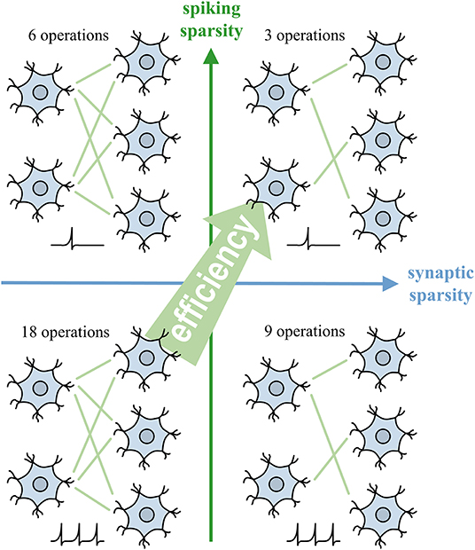
Figure 1. Spiking sparsity and synaptic sparsity facilitate the efficiency of SNN by reducing the number of synaptic operations.

The remainder of this article is organized as follows. In Section 2, the backpropagation with sparsity regularization is introduced. The suggested heterogeneous neuron dynamic model, the loss function with regularization, and the backpropagation algorithm on the flat and recurrent SNN layers are detailed. In Section 3, the rewiring based on weight and gradient and the corresponding implementation process is introduced. In Section 4, the effect of the proposed BPSR algorithm is tested by experiments, and comparisons with related works on various datasets are reported. In Section 5, we summarize this work and make a discussion.

2. Backpropagation With Sparsity Regularization

The backpropagation algorithm with regularization updates SNN parameters while improving sparsity. The spiking sparsity is implemented through backpropagation and spiking regularization. Synaptic sparsity requires the cooperation of regularization and the rewiring mechanism in Section 3. Firstly, a heterogeneous leaky integrate-and-fire (LIF) neuron dynamic model and its differential approximation are suggested. Secondly, a classification loss function with spiking regularization and synaptic regularization is introduced. Finally, the backpropagation algorithm for the flat SNN layer and the brain-like recurrent SNN layer is detailed, respectively.

2.1. Heterogeneous Leaky Integrate-and-Fire Model

As one of the most commonly used neuron models, LIF describes the dynamic process of neurons in SNN. The membrane potential of neurons increases under the stimulation of spikes and leaks spontaneously with time. When the potential reaches the spiking threshold, the neuron generates a spike and resets the membrane potential. In addition, we extend the LIF description to the spiking recurrent layer and support neurons with different time coefficients (heterogeneous), to utilize the brain-like structure and temporal features. We hierarchically describe the SNN. For the n-th layer, the LIF process can be described by equations in the discrete-time domain:

$\begin{array}{ll}{u}_i^t=u_i^{t-1}·{\tau }_i·\overline{s_i^{t-1}}+{\displaystyle \sum _{j\in {𝕃}^{\text{n}-1}}}{w}_{ij}·x_j^t+{\displaystyle \sum _{k\in {𝕃}^{\text{n}}}}{w}_{ik}·s_k^{t-1}+b_i,i\in {𝕃}^{\text{n}}& (1)\end{array}$

$\begin{array}{ll}{s}_i^t=g(u_i^t-U_{th})& (2)\end{array}$

where $u_i^t$ is the membrane potential of i-th neuron in layer 𝕃ⁿ at time t (𝕃ⁿ represents the set of neurons in the n-th layer). $s_i^t\in \left\{0,1\right\}$ is a boolean value where $s_i^t=1$ denotes a spike activity. $\overline{s_i^{t-1}}$ means to take a logical ‘not' operation on $s_i^{t-1}$. τ_i ∈ [0, 1] is the leakage time coefficient, which achieves neuronal heterogeneity. This allows the neuron model to be heterogeneous and facilitates temporal feature extracting. Multiply $u_i^{t-1}$ by ${\tau }_i·\overline{s_i^{t-1}}$ controls whether the membrane potential leaks by τ_i or drops to the resting potential 0. The neuron bias is denoted by b_i, leading to self-excitation or self-suppression. $x_j^t$ is the input spike from the j-th neuron in layer 𝕃ⁿ⁻¹. It should be noted that, for the calculation of layer 𝕃ⁿ⁺¹, $x:=s_i^t,i\in {𝕃}^{\text{n}}$. In this way, spikes are transmitted layer by layer. As shown in Figure 2, the SNN layer can be classified as Figure 2A the flat layer and Figure 2C the recurrent layer. For the flat layer, w_ij represents inter-layer synapse from the j-th neuron in layer 𝕃ⁿ⁻¹ to i-th neuron in layer 𝕃ⁿ. For the recurrent, w_ik is appended to indicate intra-layer synapse inside layer 𝕃ⁿ, which has the ability to extract temporal features due to the brain-like structure. The Heaviside function g(·) generates a spike when $u_i^t$ is greater than or equal to the spiking threshold U_th. Heaviside function and the adopted differential approximation are expressed as:

$\begin{array}{ll}g(x)=\{\begin{array}{cc}1,& x\ge 0\\ 0,& x<0\end{array},g^{\prime }(x)=\frac{\alpha }{\sqrt{\pi }}{e}^{-{\alpha }^2{x}^2}& (3)\end{array}$

Backpropagation requires a differentiable path. The derivative of the Heaviside function g(·) is the Dirac function δ(·), whose value is +∞ at 0 and impossible to perform the calculation. Thus, the Gaussian function is introduced as the differential approximation of the Heaviside function, where α controls the shape of the function.

FIGURE 2

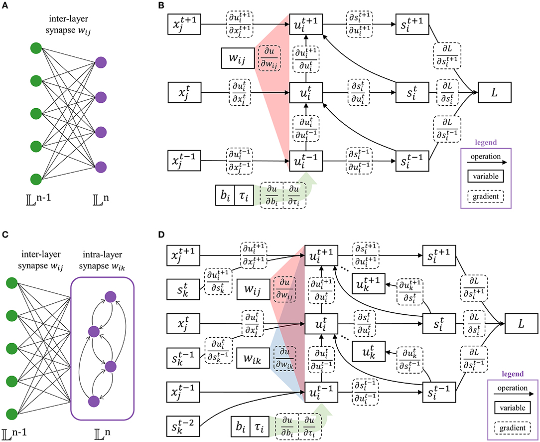
Figure 2. The structure of the SNN layer contains (A) the flat layer with only inter-layer synapses (w_ik = 0), and (C) the recurrent layer with intra-layer synapses (w_ij ≠ 0). The corresponding computational graphs are (B,D), respectively. The legends of arithmetic operations, neuron state variables, and gradients are marked in the lower right corner.

2.2. Loss Function With Sparsity Regularization

The loss function measures the error for a classification task and the sparsity of SNN, which is defined as follows. The first term measures the classification error through softmax and cross-entropy functions. The second and third terms achieve spiking sparsity and synaptic sparsity, respectively.

$\begin{array}{ll}L={\displaystyle \underset{\text{classification error}}{{\displaystyle \underbrace{-{\displaystyle \sum _c}{y}_{c}log(p_c)}}}}+{\displaystyle \underset{\text{spiking sparsity}}{{\displaystyle \underbrace{\frac{{\lambda }_s}{2}{\displaystyle \sum _{i\notin {𝕃}^{\text{N}}}}{\displaystyle \sum _t}{\Vert s_i^t\Vert }_2^2}}}}+{\displaystyle \underset{\text{synaptic sparsity}}{{\displaystyle \underbrace{{\lambda }_w{\displaystyle \sum _{w\in {𝕃}^{\text{n}}}}{\Vert w\Vert }_1}}}}& (4)\end{array}$

$\begin{array}{ll}{p}_c=\text{softmax}(k·{\displaystyle \sum _t}{s}_c^t)=\frac{exp({\displaystyle {\sum }_t}k·s_c^t)}{{\displaystyle {\sum }_{i\in {𝕃}^{\text{N}}}}exp({\displaystyle {\sum }_t}k·s_i^t)}& (5)\end{array}$

where y_c is the ground-truth label of one-hot coding for the c-th class. p_c is the predicted probability given by the output layer 𝕃^N. p_c is calculated by summing of the output spikes, multiplied by factor k, and then processing by softmax function. The factor $k=\frac{10}{T}$ corrects the softmax error by scaling the sum of spikes in the time window T. λ_s is the coefficient of l₂ regularization for spiking sparsity. It takes effect on the spikes of the SNN layer, except for the output layer to ensure classification accuracy. λ_w is the coefficient of l₁ regularization for the sparsity of synaptic weight, which is effective for all layers of the SNN.

The regularizations of spiking sparsity and synaptic sparsity have similar forms and can promote each other. But in essence, their mechanism is different (as shown in Table 1). The goal of spiking regularization is to reduce FR while ensuring guaranteed accuracy. Therefore, the regular term adjusts the parameters w_ij, w_ik, b_i, and τ_i to punish dense spikes. Synaptic regularization works together with the rewiring mechanism in Section 3 to realize pruning of the weight w_ij and w_ik. The gradient of spiking regularization is calculated by the chain rule. When either input spike $x_j^t$ or output spike $s_i^t$ is 0, the spiking regularization will not be affected. The gradient of synaptic regularization is calculated directly, and it works continuously until the weight is set to 0. As regularization, both of them improve network performance by preventing overfitting. The difference is that the principle of spiking regularization is simplifying feature expression to improve generalization ability. While synaptic regularization and rewiring work together to take effect by reducing the dimensionality of the parameter space.

TABLE 1

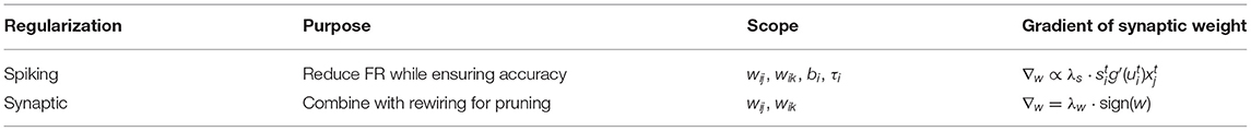
Table 1. Comparison between spiking and synaptic regularization.

2.3. Backpropagation in Flat Layer

The error information is propagated through the gradient and the parameters of SNN are updated accordingly. Therefore, it is necessary to derive the gradient of the loss function to each parameter. There are only inter-layer synaptic connections in the flat layer structure and w_ik = 0. The computational graph of the flat layer and the corresponding gradient path are shown in Figure 2B. For the output layer 𝕃^N, the partial derivative ∂L/∂s can be directly calculated. For the non-output layer (𝕃ⁿ, n < N), the partial derivative ∂L/∂s is the ∂L/∂x of the following layer, plus the spiking regularization term.

$\begin{array}{ll}\frac{\partial L}{\partial s_i^t}=\{\begin{array}{l}{p}_i-y_i,i\in {𝕃}^{\text{N}}\\ \frac{\partial L}{\partial x_j^t}+{\lambda }_s·x_j^t,i\in {𝕃}^{\text{n}},j\in {𝕃}^{\text{n}+1},n<N\end{array}& (6)\end{array}$

The spike $s_i^t$ is a function of the membrane potential $u_i^t$, and the membrane potential changes over time. Although $u_i^t$ is a function of $s_i^{t-1}$ in Equation (1), $s_i^{t-1}$ only gates the information flow in potential along time. Unlike $u_i^t$ accumulating information to $s_i^t$, or $x_j^{t-1}$ passing w_ij of information to $u_i^t$, $s_i^{t-1}$ has no information contribution to $u_i^t$. Thus, $\partial u_i^t/\partial s_i^{t-1}$ is ignored in backpropagation. $\partial L/\partial u_i^t$ is expressed as:

$\begin{array}{ll}\frac{\partial L}{\partial u_i^t}=\{\begin{array}{l}\frac{\partial L}{\partial s_i^t}·\frac{\partial s_i^t}{\partial u_i^t}=\frac{\partial L}{\partial s_i^t}·g^{\prime }(u_i^t-U_{th}),t=T\\ \frac{\partial L}{\partial s_i^t}·\frac{\partial s_i^t}{\partial u_i^t}+\frac{\partial L}{\partial u_i^{t+1}}·\frac{\partial u_i^{t+1}}{\partial u_i^t}\\ =\frac{\partial L}{\partial s_i^t}·g^{\prime }(u_i^t-U_{th})+\frac{\partial L}{\partial u_i^{t+1}}·{\tau }_i·\overline{s_i^t},t<T\end{array}& (7)\end{array}$

The part of t < T in Equation (7) takes into account all the errors after time t through iterative calculation and reduces the algorithm complexity to O(t). Assuming the direct error from the loss function at time t is ${\epsilon }^t=\partial L/\partial s_i^t·\partial s_i^t/\partial u_i^t$. Figure 3 shows how the influence from the subsequent time is calculated by one addition and multiplication when t = T, T−1, T−2.

FIGURE 3

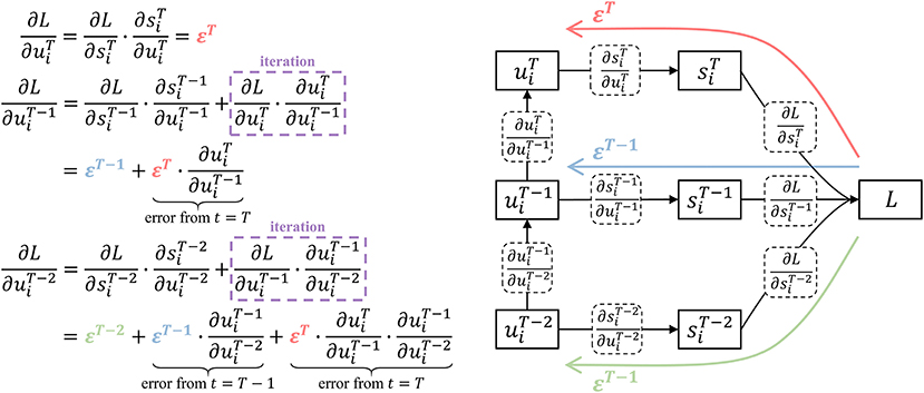
Figure 3. Iterative calculation with linear algorithm complexity. At time T, the potential error comes from the direct error ε^T. At time T − 1, the potential error includes the direct error ε^T−1 and the backpropagation of ε^T. At time T − 2, the influence of ε^T, ε^T−1, ε^T−2 are taken into account through iterative calculation, which only requires one addition and multiplication.

Once the gradient to $u_i^t$ is obtained, the gradients to each parameter and input spike are easy to calculate by the following equations, where i belongs to layer 𝕃ⁿ and T is the time window. The initial value $u_i^0=s_i^0=0$. Learning shared parameters such as convolution weights or homogeneous leakage coefficients can be realized by summing the gradient of shared weight. Potential changes well beyond the threshold have no effect, so excessively large w_ij and b_i are meaningless and clamped to [−U_th, +U_th] accordingly. τ is also limited to its range of values [0, 1].

$\begin{array}{ll}\frac{\partial L}{\partial x_j^t}={\displaystyle \sum _{i\in {𝕃}^{\text{n}}}}\frac{\partial L}{\partial u_i^t}·\frac{\partial u_i^t}{\partial x_j^t}={\displaystyle \sum _{i\in {𝕃}^{\text{n}}}}\frac{\partial L}{\partial u_i^t}·w_{ij}& (8)\end{array}$

$\begin{array}{l}\frac{\partial L}{\partial w_{ij}}={\displaystyle \sum _{t=1}^T}\frac{\partial L}{\partial u_i^t}·\frac{\partial u_i^t}{\partial w_{ij}}+{\lambda }_w·\text{sign}(w_{ij})\\ ={\displaystyle \sum _{t=1}^T}\frac{\partial L}{\partial u_i^t}·x_j^t+{\lambda }_w·\text{sign}(w_{ij})& (9)\end{array}$

$\begin{array}{ll}\frac{\partial L}{\partial b_i}={\displaystyle \sum _{t=1}^T}\frac{\partial L}{\partial u_i^t}·\frac{\partial u_i^t}{\partial b_i}={\displaystyle \sum _{t=1}^T}\frac{\partial L}{\partial u_i^t}& (10)\end{array}$

$\begin{array}{ll}\frac{\partial L}{\partial {\tau }_i}={\displaystyle \sum _{t=1}^T}\frac{\partial L}{\partial u_i^t}·\frac{\partial u_i^t}{\partial {\tau }_i}={\displaystyle \sum _{t=1}^T}\frac{\partial L}{\partial u_i^t}·u_i^{t-1}·\overline{s_i^{t-1}}& (11)\end{array}$

2.4. Backpropagation in Recurrent Layer

The intra-layer synaptic connections exist in the recurrent layer, i.e., w_ik ≠ 0. This makes the computational graph of the recurrent layer and the gradient path are different from the flat layer, which are shown in Figure 2D. The calculation method of the partial derivative $\partial L/\partial s_i^t$ still follows Equation (6). Considering the intra-layer connection within the recurrent, $\partial L/\partial u_i^t$ is modified to:

$\begin{array}{ll}\frac{\partial L}{\partial u_i^t}=\{\begin{array}{l}\frac{\partial L}{\partial s_i^t}·\frac{\partial s_i^t}{\partial u_i^t}=\frac{\partial L}{\partial s_i^t}·g^{\prime }(u_i^t-U_{th}),t=T\\ \frac{\partial L}{\partial s_i^t}·\frac{\partial s_i^t}{\partial u_i^t}+\frac{\partial L}{\partial u_i^{t+1}}·\frac{\partial u_i^{t+1}}{\partial u_i^t}+{\displaystyle \sum _{k\in {𝕃}^{\text{n}}}}\frac{\partial L}{\partial u_k^{t+1}}·\frac{\partial u_k^{t+1}}{\partial s_i^t}·\frac{\partial s_i^t}{\partial u_i^t}\\ =\left[\frac{\partial L}{\partial s_i^t}+{\displaystyle \sum _{k\in {𝕃}^{\text{n}}}}\frac{\partial L}{\partial u_k^{t+1}}·w_{ki}\right]·g^{\prime }(u_i^t-U_{th})\\ +\frac{\partial L}{\partial u_i^{t+1}}·{\tau }_i·\overline{s_i^t},t<T\end{array}& (12)\end{array}$

Note that for the intra-layer synaptic weight, we swap the subscripts of the input and the output neurons (denoted as w_ki). The above equation is still an iterative calculation with time complexity of O(t). The calculation of the gradient of each parameter is still consistent with Equation (8)–(9). As a supplement, ∂L/∂w_ik can be calculated by the following equation, where i and k both belong to layer 𝕃ⁿ and the initial value $s_k^0=0$.

$\begin{array}{l}\frac{\partial L}{\partial w_{ik}}={\displaystyle \sum _{t=1}^T}\frac{\partial L}{\partial u_i^t}·\frac{\partial u_i^t}{\partial w_{ik}}+{\lambda }_w·\text{sign}(w_{ik})\\ ={\displaystyle \sum _{t=1}^T}\frac{\partial L}{\partial u_i^t}·s_k^{t-1}+{\lambda }_w·\text{sign}(w_{ik})& (13)\end{array}$

In this way, the required gradients are obtained. Errors can be passed down layer by layer. Each network parameter can be updated by various general ANN parameter optimization algorithms, such as stochastic gradient descent (SGD), adaptive momentum estimation (Adam) (Kingma and Ba, 2014) or Adam with decoupled weight decay (AdamW) (Loshchilov and Hutter, 2017).

2.5. Post-training Quantization

Fixed-point quantification can compress the storage overhead of SNN, and achieve higher computational efficiency by replacing floating-point arithmetic with fixed-point arithmetic. We use PTQ to quantify parameters, avoiding the overhead of re-learning. After learning, PTQ quantizes w and b into n-bit fixed-point numbers, where the fraction length is n - 1 and the signedness is 1-bit. This allows synaptic operations to be performed through fixed-point addition instead of floating-point addition. τ is rounded to 2^−m, so that the multiplication on the potential is replaced by m-bit right shift operation. PTQ brings optimization of storage overhead and energy consumption under the condition of limited accuracy loss.

3. Rewiring Based on Weight and Gradient

Rewiring mechanism prunes and grows synapses based on synaptic weights and gradients to improve synaptic sparsity. Synaptic weights are constantly decreasing in learning through synaptic regularization. When the |w| is less than the pruning threshold Θ_w (Equation 14), it means that the influence on the post-synaptic neuron is negligible and synapse can be pruned (Figure 4A). Moreover, the pruned synapses have a chance to reconnect through growth. The gradient of the synaptic weight represents a trend of growth. The momentum m is the exponential moving averaging of the synaptic gradient ∇_w, where β_m is the coefficient of moving average. The m measures the strength of the growth trend after smoothing fluctuations. When the m is large enough to satisfy Equation (15), the synapse grows as shown in Figure 4B. The growth conditions include a constant threshold Θ_m and a distance term scaled by the ratio μ_m, where c_i and c_j represent the spatial coordinates of two neurons. The above condition means that establishing a longer-range synaptic connection requires a stronger growth trend. Dynamic rewiring is coupled with the learning process, using pruning and growth to improve sparsity and ensure performance. SNN is finally stable between rewiring and parameter optimization and acquires a sparse and efficient network structure.

$\begin{array}{ll}\text{pruning }:|w|<{\Theta }_w& (14)\end{array}$

$\begin{array}{l}\text{growth }:|m|>{\Theta }_m·\left(1+{\mu }_m{\Vert c_i-c_j\Vert }_2^{1/2}\right),\\ m:=m+(1-{\beta }_m){\nabla }_w& (15)\end{array}$

The rewiring mechanism works together with backpropagation and parameter optimization. The pseudo-code (Algorithm 1) takes layer 𝕃ⁿ as an example to illustrate how to implement the proposed BPSR algorithm with matrix operation. The input spike matrix X and the gradient matrix of output spike Δ_S are required. ${{N}}^n$ represents the number of neurons in layer 𝕃ⁿ and T is the time window. The shape of X is ${{N}}^{n-1}\times T$. The gradient Δ_S with shape of ${{N}}^n\times T$ can be backpropagated by the following layer through Equation (6). The notation [t] is used to represent the matrix slice in the time dimension. The algorithm generates the output spike S and the gradient of the input spike Δ_X, and ensures to update the synaptic weight matrix W, bias matrix B and, leakage coefficient matrix ${T}$. For the flat layer, we mark the synaptic weight as W = W_ij. For the recurrent layer, the synaptic weight matrix is the concatenation W = [W_ij|W_ik]. In the initial stage, the weight matrix W is set to obey Gaussian distribution ${N}(0,1)$. The bias matrix B is initialized to uniform distribution ${U}(0,1)$. The leakage coefficient matrix ${T}$ is set to an empirical value of 0.5. The coordinates of neurons C are set to the random distribution in the unit cube. Especially, Kaiming initialization (He et al., 2015) is applied to the convolutional layer. The coordinates of neurons C are set to the random distribution in the unit cube. The forward and backpropagation processes are described in the previous sections. In the rewiring, Prun and Grow are two boolean matrices, denoting the synapses that meet the conditions 14 and 15. The boolean matrix Mask indicates the existing synapses after rewiring. Logical operations “and” and “or” achieve prune and grow, respectively. The W and Δ_W is superimposed by Mask. Finally, all parameters are updated through the ANN optimization algorithm and clamped.

FIGURE 4

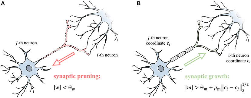
Figure 4. (A) The weight of synapse w controls the synaptic pruning. (B) The momentum of the synapse gradient m controls the synaptic growth.

ALGORITHM 1

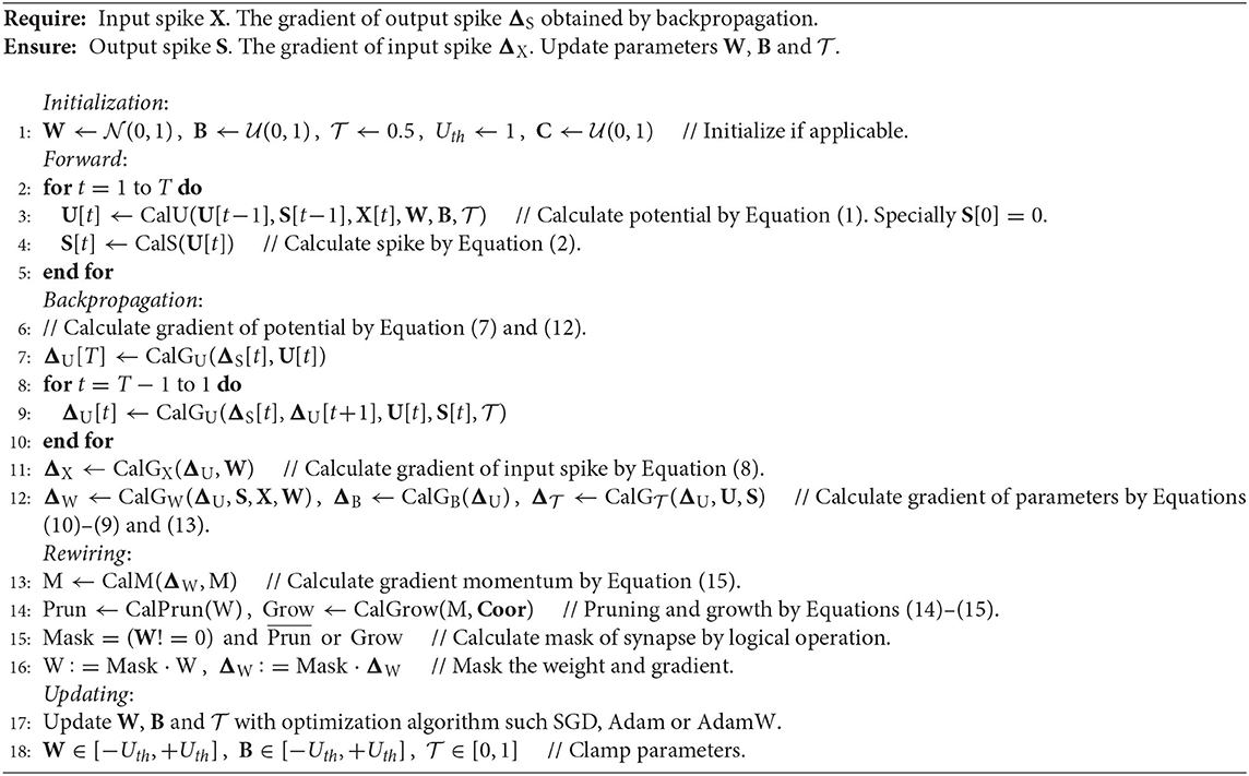
Algorithm 1: The BPSR implementation of layer 𝕃ⁿ.

4. Experimental Results

The proposed BPSR is implemented by PyTorch (Paszke et al., 2019) and runs on a CPU of AMD Ryzen-3970X and a GPU of NVIDIA RTX-3080. Various visual datasets and sensor datasets are used in the experiments. MNIST is a static digital dataset and can be transformed into a spiking dataset by rate coding and rank order coding. Rate coding (Figure 5A) takes pixel intensity as the probability and performs Bernoulli sampling in the time domain to produce spikes. Rank order coding (Figure 5B) convert higher values to earlier spikes, which is a kind of temporal sparse coding. Unlike rate coding, the spiking timing in rank order is meaningful. This requires the SNN to have the capacity for temporal processing. N-MNIST is a spiking version of MNIST and is acquired by the dynamic vision sensor (DVS). It is widely used in SNN research due to event-driven and neuromorphic. CIFAR10 is another static visual dataset for object classification of color images. We employ the encoding layer proposed by Wu et al. (2019) to convert floating values to spikes. MIT-BIH is an arrhythmia dataset that includes 48 sets of electrocardiographs (ECG). The level-crossing (LC) sampling (Marisa et al., 2017) converts signal into spike. 2-channel ECG generates 4-channel spiking input suitable for SNN, as shown in Section 4.1. The gas sensor dataset is the record from a chemical detection platform in a wind tunnel facility in response to ten high-priority chemical gaseous substances. The 72-channel sensing signal is encoded by rank order to obtain the spiking input.

FIGURE 5

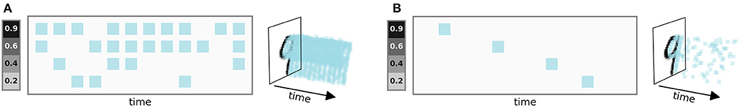
Figure 5. The principle of (A) rate coding and (B) rank order coding, and the spike sequence of an MNIST image after coding.

4.1. Coding Method and Feature Visualization

A 5-class ECG task is used to show how SNN processes temporal information. The SNN model resented in Figure 6A is the recurrent MLP (rMLP) of “r18 - fc8 - fc5”, where “r” denotes the recurrent layer and ‘fc' denotes the fully connected layer. Figure 6B demonstrates the original ECG signal and the spiking sequence after LC sampling. The 2 channels of the displayed record 102 are modified lead V2 and V5, and other records may contain modified limb lead II (MLII). Bipolar spikes are generated on the edge of signal changes in each channel. In this way, the spike reflects the changing trend of the signal. 4-channel spikes input to the recurrent layer for temporal feature processing. In the right of Figure 6C, the output FR curve of the recurrent layer under different input FR is plotted channel by channel. Neurons can be classified into low-pass, high-pass, band-pass and composite characteristics according to different filter effects. The left of Figure 6C shows the spike output of the recurrent layer and its influence on the prediction result. All neurons have a positive effect (green) on the prediction results, except for neuron 11 marked by the black box. In addition, neurons 0, 10, and 15 make more contributions, revealing that the corresponding frequency features are more important for predicting this class. Figure 6D is the spike output of the hidden layer. The role of this layer is the feature mapping before prediction. All neurons also make a positive effect except for one neuron. The final prediction result (Figure 6E) is the spike sum of 5 output neurons and is normalized to probability. It can be seen that the SNN makes the correct prediction for a normal heartbeat.

FIGURE 6

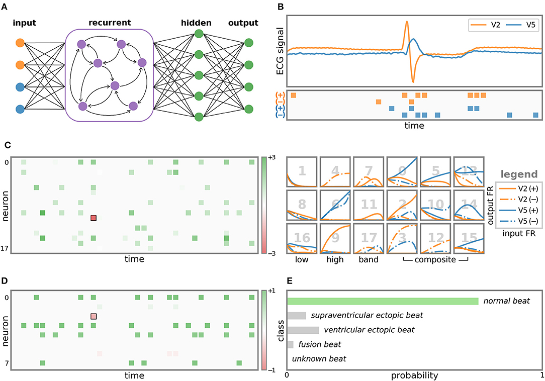
Figure 6. Visualization of LC sampling and each layer of SNN. (A) The structure of the SNN model. (B) The ECG signal and the input spikes after LC sampling. (C) Output spikes and corresponding FR response curves of 18 neurons in the recurrent layer. The coordinates of the spikes represent the occurrence time and the neuron index. The color indicates the impact on the prediction result, where green is positive and red is negative. Response curves are plotted channel-by-channel. The x-axis and y-axis are the input and output FR, respectively. The 18 neurons are classified according to the filter effect, and the corresponding neuron index is marked in gray number. The output spikes of the hidden layer are drawn on (D), and the predicted probability for the 5 ECG classes is shown on (E).

4.2. Algorithm Efficiency

The runtime and memory overhead reflect the efficiency of the algorithm, the accuracy and convergence epoch number prove its effectiveness. The proposed BPSR is compared with the other three SNN gradient descent algorithms, namely DECOLLE, STBP, and graph-based STBP (G-STBP) (Yan et al., 2021a). The four algorithms are all implemented based on PyTorch and accelerated by the GPU to get a fair comparison. The MNIST is encoded by rate coding as the time window T and the learning batch size is set to 32. The SNN model is a three-layer multilayer perceptron (MLP), where the size of the input layer is 784 and the output layer is 10. The number of neurons in the hidden layer (${{N}}^1$) is a variable in the experiment. Figure 7 shows the algorithm runtime of a single epoch, the graphic memory overhead on the GPU, the accuracy with rate coding in different situations, and the number of epochs required for SNN learning to reach convergence. It can be seen that G-STBP has the smallest runtime in any case, also accompanied by the highest memory overhead. G-STBP describes the network as a whole adjacency graph. This allows backpropagation to be carried out on the entire network together instead of layer by layer, but the inter-layer connection is expressed as zero resulting in memory overhead. BPSR simplifies the storage and calculation burden of intermediate quantities through iterative calculations, bringing faster runtime (2.1× than STBP) and smaller memory overhead. BPSR also achieves the highest accuracy in all cases, with the second most convergence epoch, verifying its effectiveness.

FIGURE 7

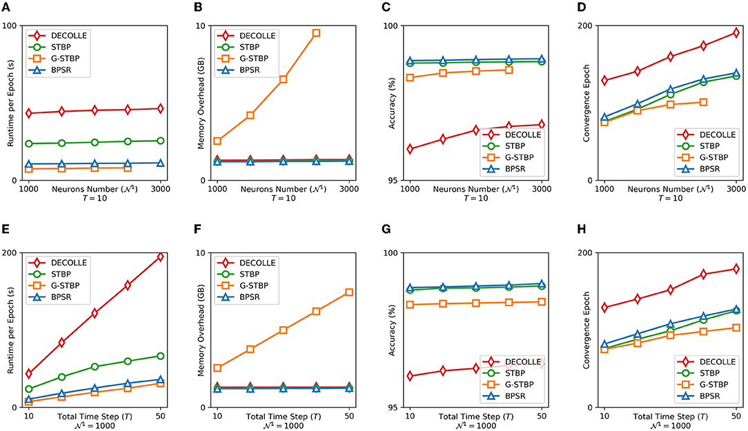
Figure 7. (A) Runtime, (B) graphic memory overhead, (C) accuracy, and (D) convergence epoch of four learning algorithms are counted under the different number of hidden layer neurons ${{N}}^1$. Panels (E–H) are the corresponding indicator under the different length of time window T.

4.3. Spiking Sparsity and Synaptic Sparsity

The effect of spiking sparsity regularization is tested on the MNIST dataset encoded by rank order. The used SNN model is rMLP of “r1000 - fc100 - fc10.” The accuracy and average FR of the test set are counted under different spiking regularization coefficients λ_s. The count of FR excludes the input spike because it is controlled by the encoding method rather than the regularization. It can be seen from Figure 8A that FR decreases as the spiking regularization coefficient λ_s increases. Spiking regularization forces SNN to express information with fewer spikes. Through appropriate λ_s, the SNN can achieve high accuracy with low computation overhead in the inference. Moreover, the accuracy is improved with the decrease of FR when ${\lambda }_s\in \left[0,10^{-7}\right]$. One reason is that SNN learning is a process of FR reduction. As shown in Figure 8B, the accuracy and FR are approximately inversely related during the learning process. SNN learns important features by suppressing redundant information. Setting a high initial threshold (U_th = 10) causes the FR to increase first and then become an inversely proportional learning process. Inappropriately high threshold (U_th = 12) can even lead to network divergence. The learning curve in Figure 8C verifies that spiking regularization can prevent overfitting. Under the same training error, the SNN with spike regularization achieves improved test accuracy and shows better generalization.

FIGURE 8

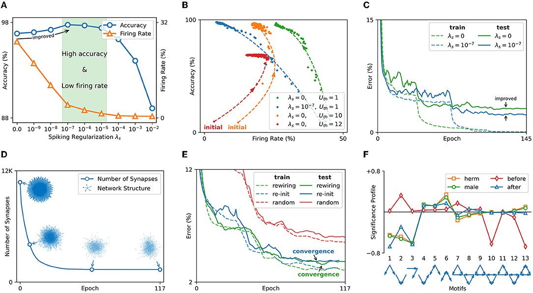
Figure 8. (A) The test accuracy and FR under different spiking regularization coefficients λ_s. (B) Accuracy and FR change law in the learning process. (C) Learning curves under different λ_s (after smoothing filtering). (D) The number of synapses and network structure changes in the recurrent layer. (E) The learning curve with and without rewiring mechanism (after smoothing filtering). (F) Significance profile of C. elegans nervous system and the gas sensor network.

The effect of synaptic sparsity regularization is tested on the gas sensor dataset and the learned SNN structure is compared with the nervous system of Caenorhabditis elegans (C. elegans). The neuron connection graph of C. elegans has been fully studied (Cook et al., 2019). The hermaphrodite and the male have 302 neurons and 385 neurons, respectively. 83 sensory neurons and 81 interneurons are the same for all genders. The tested SNN model is “r81 - fc36 - fc10.” The input layer and the first hidden layer have a similar number of neurons as the C. elegans, which is convenient for structural comparison. SNN learns under synaptic regularization coefficient λ_w = 0.01. The line in Figure 8D shows the number of synapses in the input layer and the first hidden layer. The point cloud plots the network structure (topological connection) during the rewiring process. After 117 epochs, the network can be 8× in the recurrent layer. In Figure 8E, the above network obtained by rewiring is re-initialized to evaluate the convergence speed. SNN with the same number of synapses but a random structure is also tested. Experiment shows that the SNN without rewiring will reach the lowest error 4 epochs earlier than the SNN with rewiring. SNN with random structures has higher errors, demonstrating the effect of rewiring.

The efficacy of rewiring is further verified by significance profile (SP) (Milo et al., 2004), a method of analyzing the similarity of network structure. It measures the structural characteristics of the network by comparing the number of occurrences of different induced subgraphs (i.e., motifs) in the network. The possible connection modes between the three nodes are used as 13 motifs. A set of random networks is generated as the reference based on the degree sequence of the network to be tested. The numbers of occurrences of 13 motifs in the network to be tested and the random network set are recorded as the 13-dimensional vector N_test and vector set N_rand, respectively. The SP is the vector normalization of $({\mathbf{\text{N}}}_{test}-{\overline{\mathbf{\text{N}}}}_{rand})/\text{std}({\mathbf{\text{N}}}_{rand})$. The SP of hermaphrodite (herm) and male C. elegans, and the SP of SNN before and after learning are plotted in Figure 8F. It can be seen that the hermaphrodite and the male C. elegans have the same structural characteristics. After BPSR learning, the structure of SNN is more similar to the nervous system of C. elegans, which means that the rewiring mechanism can generate an effective and bionic network structure.

4.4. Evaluation of Performance

Table 2 provides the network structure and hyper-parameters used in the various experiments below. Convolutional indicator “8c5/2” means kernel size 5, output channel 8 and stride 2. “r” and “fc” denote the recurrent layer and the fully connected layer, respectively. [·] means a residual block (He et al., 2016). For convolutional neurons, τ is homogeneous and shared while learning. For neurons in other layers, τ is heterogeneous.

TABLE 2

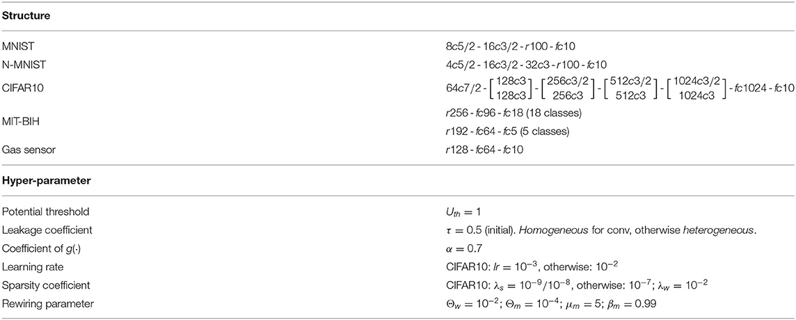
Table 2. SNN structures and hyper-parameters setup.

4.4.1. MNIST Dataset

Table 3 shows the comparison results of the proposed BPSR and related SNN works on the MNIST dataset. The pooling is taken into account of the number of synapses, and shared weight in the convolution is repeatedly added. The introduction of recurrent layers enhances accuracy but brings additional overhead, which is further improved by sparsity regularization. Compared to other sparse networks using pruning, the proposed BPSR acquired the least number of synapses, with the best spiking sparsity except for G-STBP. Floating-point operations (FLOPs) show the computational overhead of SNN in the learning and inference process. Conversion-based algorithm (Diehl et al., 2015) learns parameters through ANN, avoiding the backpropagation in the time window. It has the lowest learning FLOPs and high accuracy (the conversion cost is underlined and only occurs once after learning). Plasticity-based algorithm is generally considered to be efficient due to local learning rules. However, Diehl and Cook (2015) used a large network to improve the accuracy, resulting in the learning burden. Gradient-based algorithms have high backpropagation overhead but also bring performance optimization. Wu et al. (2018) and Yan et al. (2021a) have improved the SNN with the goal of better accuracy and sparser spikes, respectively. The proposed BPSR achieves a low learning overhead due to its extremely sparse network. Moreover, rank order coded data has a higher learning difficulty due to sparse temporal representation. The accuracy of BPSR is only 0.8–1.1% lower than rate coding, with a 30× inference overhead advantage.

TABLE 3

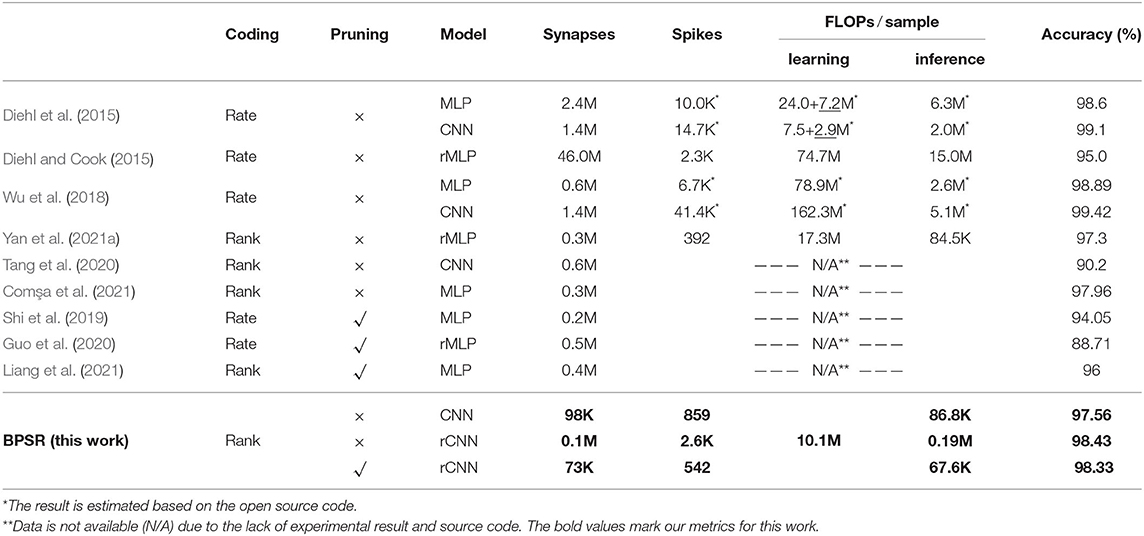
Table 3. Comparison of different spiking models on MNIST dataset.

Networks such as BNN and AdderNet improve energy efficiency by reducing computational overhead, which is similar to SNN. We also compare the performance of the proposed BPSR and other ANN in Figure 9. The network structure used is LeNet5 and their variant. As mentioned in the original work, batch normalization (BN) (Ioffe and Szegedy, 2015) is introduced to improve accuracy. The involved operations include floating-point multiplication (FL-MUL), floating-point addition (FL-ADD), fixed-point addition (FI-ADD), and bitwise operation (BIT-OP). The network energy consumption in inference is counted by normalization. FL-ADD is considered as unit overhead. FL-MUL is estimated to be 4× of floating-point addition (Cheng et al., 2019), and FI-ADD is estimated to be 20% of FL-ADD (Finnerty and Ratigner, 2017). The overhead of BIT-OP is negligible.

FIGURE 9

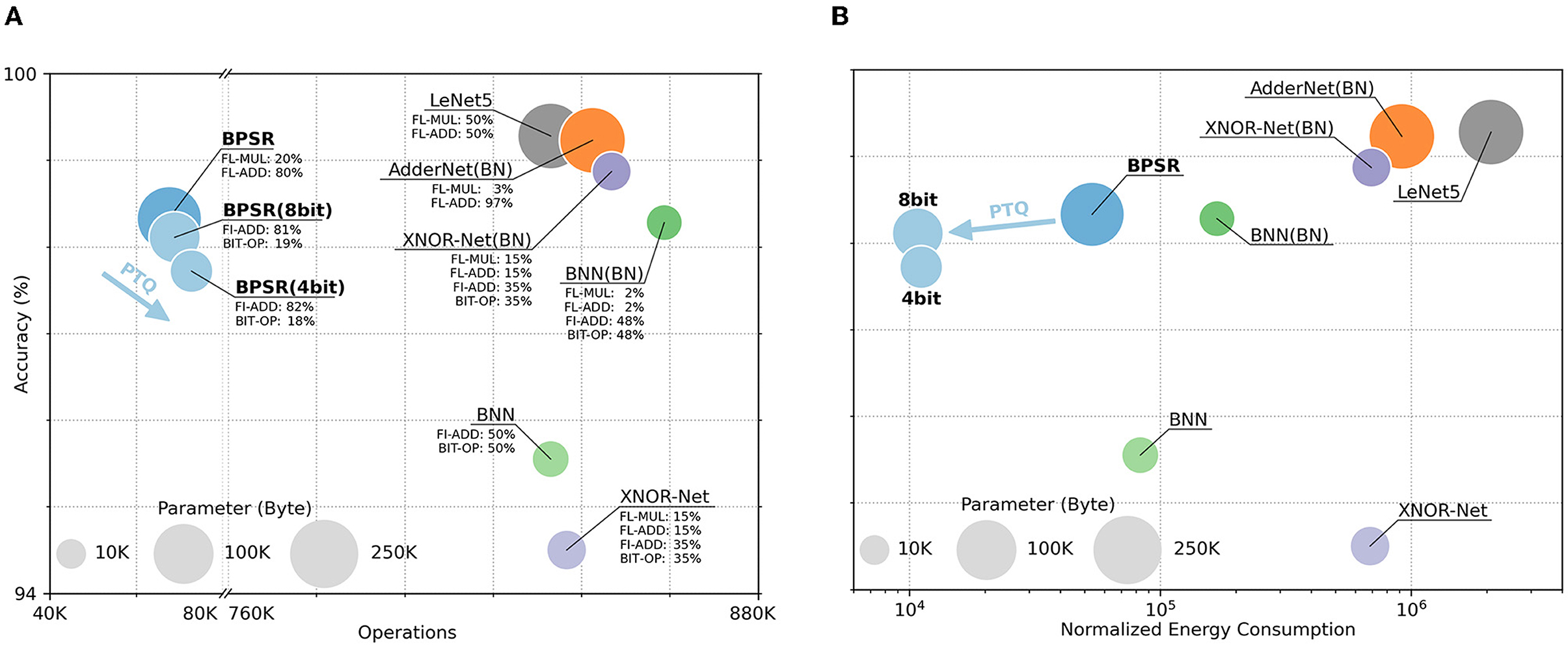
Figure 9. Accuracy, operations, normalized energy consumption, and parameter size of different networks. The area of the circle represents the storage overhead of the parameters. The y-coordinate of the center represents the network accuracy. The x-coordinate represents (A) the number of operations and (B) the energy consumption of each inference. The proportions of different operations are marked in (A). Additionally, the x-axis of (a) is folded and the x-axis of (B) is logarithmic.

Under the same structure, AdderNet reduces the computational cost by approximating multiplication by addition. BNN and XNOR-Net further reduce storage burden and energy overhead through bitwise operations. The proposed BPSR achieves optimized energy consumption through lightweight structure and sparse spike while ensuring accuracy. PTQ quantizes the parameters of SNN to 8-bit or 4-bit, and further uses fixed-point addition and bitwise right shift instead of floating-point addition and floating-point multiplication to reduce the energy cost. After PTQ, the proposed BPSR reaches 15 ~ 60× energy efficiency than BNN or XNOR-Net, with a 0.22–0.61% accuracy drop of unquantized SNN.

4.4.2. N-MNIST Dataset

Table 4 shows the comparison of N-MNIST. Event-driven N-MNIST is usually converted to frame-based data. Time step T matches the time length of the frame sequence. Most networks take few time steps, except Kaiser et al. (2020) which uses 60 steps to warm up the network and 240 steps to learn and infer. Kaiser et al. (2020) uses a shallow network, but the readout layer followed by each regular layer greatly increases the synaptic overhead. The network used by Vaila et al. (2019) is a mixture of ANN and SNN, and the prediction results are given by SVM. Wu et al. (2019) uses the deepest network and most synapses to get the best accuracy. BPSR has minimal synaptic overhead and achieves the second-best accuracy. Introducing a recurrent layer improves the accuracy in the case where the number of tiny synapses grows, proving that the recurrent structure is useful for frame sequence processing.

TABLE 4

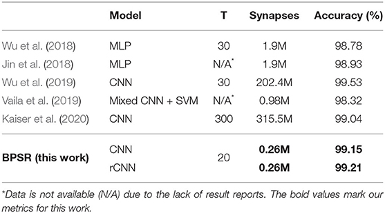
Table 4. Comparison of different spiking models on N-MNIST dataset.

4.4.3. CIFAR10 Dataset

We applied the residual SNN on CIFAR10 to verify the performance of the BPSR on the deep model. Table 5 compares BPSR with other SNN works. Sengupta et al. (2019) achieves the best accuracy on VGG16 with a conversion-based learning algorithm. However, the conversion takes 2500 time steps to rate encoding, much higher than other methods. Wu et al. (2019) uses a gradient-based learning algorithm to achieve high accuracy while keeping small time steps. Although in the work of Allred et al. (2020), the accuracy of SNN is limited by the network size, the sparsity resulting from regularization is further explored. We test BPSR on an 11-layer residual network composed of 4 residual blocks. The number of synapses is less than that of other deep networks. The proposed BPSR can reach 90.24% accuracy with the same number of spikes as Allred et al. (2020), or achieve the accuracy of 90.74% with 50% additional spike overhead.

TABLE 5

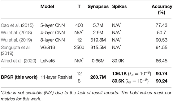
Table 5. Comparison of different spiking models on CIFAR10 dataset.

4.4.4. MIT-BIH Dataset

Table 6 are the comparison results between BPSR and related spiking models on the MIT-BIH dataset. Most of the work introduces recurrent structures such as lateral inhibition to process temporal signals. In addition, Kolağasioğlu (2018) use wavelet transform for signal preprocessing, Wu et al. (2020) adopt the gated recurrent unit (GRU), and Corradi et al. (2019) use the support vector machine (SVM) for prediction. These make the implementation no longer pure SNN. MIT-BIH dataset contains various ECG arrhythmia types with a long-tailed distribution. The classification of the fewer sample has a higher learning difficulty. Most works achieve 2-5 classification tasks by selecting subsets and merging certain classes. Kolağasioğlu (2018) and Corradi et al. (2019) take 17 or 18 classes for fine-grained classification. Thus, we used the two models 18 classes and 5 classes. BPSR can make inferences from the compressed time window (T = 40), which is more efficient. The proposed BPSR achieves the highest accuracy in fine-grained classification and coarse-grained classification. With the proposed sparsity regularization, the learned models under different classification tasks both achieve optimal synaptic sparsity.

TABLE 6

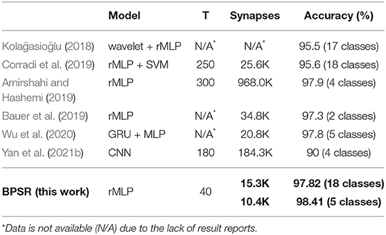
Table 6. Comparison of different spiking models on MIT-BIH dataset.

4.4.5. Gas Sensor Dataset

Table 7 shows the comparison results of BPSR and related works on the gas sensor dataset. Vergara et al. (2013) use the SVM method to obtain high accuracy. Imam and Cleland (2020) implement the spiking method on Loihi through the external plexiform layer (EPL) structure. Although this method does not perform well in network accuracy, the reported results show high robustness and biological inspiration. BPSR achieves better accuracy and synaptic overhead than related works. At the same time, the proposed SNN with sparsity regularization only needs 762 spikes per sample to achieve the inference.

TABLE 7

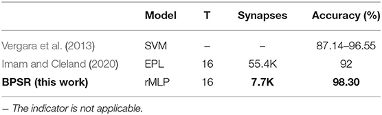
Table 7. Comparison of different models on gas senor dataset.

5. Discussion

SNN promises to realize efficient AI through its brain-inspired mechanism and spike-driven computing architecture. However, the efficiency advantage of the SNN cannot be fully exploited because of the lack of sparsity exploration. This work provides a learning algorithm, namely Backpropagation with Sparsity Regularization (BPSR), to improve efficiency through advanced spiking sparsity and synaptic sparsity. Firstly, a backpropagation algorithm with sparsity regularization is proposed to update parameters and improve sparsity. A heterogeneous LIF neuron dynamics model and a classification loss function with spiking and synaptic regularization are defined. The backpropagation algorithm of the flat and recurrent layer is detailed to calculate the gradient of each parameter. Secondly, the rewiring mechanism based on weight and gradient is proposed to improve synaptic sparsity through pruning and growth. Then, the experimental results show that the proposed BPSR has the advantages of runtime and graphic memory overhead compared with other gradient-based learning algorithms. The improved spiking sparsity can balance the accuracy and FR, and promotes the network performance by simplifying the information representation. Through the BPSR, SNN acquires a structure similar to the nervous system of C. elegans, proving its effectiveness. The proposed BPSR reaches the accuracy of 98.33% on the MNIST dataset while achieving 30× inference overhead than other SNN work and 15× energy efficiency compared to BNN after PTQ (with 0.22% accuracy drop). Finally, BPSR is also evaluated on two visual datasets (N-MNIST and CIFAR10) and two sensor datasets (MIT-BIH and gas sensor). The experimental results show comparable or superior accuracy (99.21, 90.74, 98.41, and 98.30%, respectively), with spiking sparsity and synaptic sparsity.

Data Availability Statement

The original contributions presented in the study are included in the article/supplementary material, further inquiries can be directed to the corresponding authors.

Author Contributions

YY proposed the idea and did the math and engineering work. YY, HC, and YJ designed the experiments and wrote the first draft of the manuscript. YH, ZZ, and LZ directed the projects and provided overall guidance. ZZ and LZ provided the supervision and project administration. All authors contributed to manuscript revision, read, and approved the submitted version.

Funding

This work was supported in part by the National Natural Science Foundation of China under Grants 61876039, 62076066, 62004045, and 92164301, Shanghai Municipal Science and Technology Major Projects Nos. 2021SHZDZX0103, 2018SHZDZX01, 17DZ2260900, and NSFC-STINT project No. 62011530132.

Conflict of Interest

The authors declare that the research was conducted in the absence of any commercial or financial relationships that could be construed as a potential conflict of interest.

Publisher's Note

All claims expressed in this article are solely those of the authors and do not necessarily represent those of their affiliated organizations, or those of the publisher, the editors and the reviewers. Any product that may be evaluated in this article, or claim that may be made by its manufacturer, is not guaranteed or endorsed by the publisher.

References

Akopyan, F., Sawada, J., Cassidy, A., Alvarez-Icaza, R., Arthur, J., Merolla, P., et al. (2015). Truenorth: Design and tool flow of a 65 mw 1 million neuron programmable neurosynaptic chip. IEEE Trans. Comput. Aided Design Integr. Circ. Syst. 34, 1537–1557. doi: 10.1109/TCAD.2015.2474396

CrossRef Full Text | Google Scholar

Allred, J. M., Spencer, S. J., Srinivasan, G., and Roy, K. (2020). Explicitly trained spiking sparsity in spiking neural networks with backpropagation. arXiv [Preprint]. arXiv:2003.01250. Available online at: https://arxiv.org/pdf/2003.01250.pdf (accessed March 2, 2020).

Google Scholar

Amirshahi, A., and Hashemi, M. (2019). ECG classification algorithm based on STDP and R-STDP neural networks for real-time monitoring on ultra low-power personal wearable devices. IEEE Trans. Biomed. Circ. Syst. 13, 1483–1493. doi: 10.1109/TBCAS.2019.2948920

PubMed Abstract | CrossRef Full Text | Google Scholar

Bartol, T. M. Jr., Bromer, C., Kinney, J., Chirillo, M. A., Bourne, J. N., Harris, K. M., et al. (2015). Nanoconnectomic upper bound on the variability of synaptic plasticity. eLife, 4:e10778. doi: 10.7554/eLife.10778

PubMed Abstract | CrossRef Full Text | Google Scholar

Bauer, F. C., Muir, D. R., and Indiveri, G. (2019). Real-time ultra-low power ECG anomaly detection using an event-driven neuromorphic processor. IEEE Trans. Biomed. Circ. Syst. 13, 1575–1582. doi: 10.1109/TBCAS.2019.2953001

PubMed Abstract | CrossRef Full Text | Google Scholar

Białas, M., and Mańdziuk, J. (2021). Spike-timing-dependent plasticity with activation-dependent scaling for receptive fields development. IEEE Trans. Neural Netw. Learn. Syst. 1–14. doi: 10.1109/TNNLS.2021.3069683

PubMed Abstract | CrossRef Full Text | Google Scholar

Cao, Y., Chen, Y., and Khosla, D. (2015). Spiking deep convolutional neural networks for energy-efficient object recognition. Int. J. Comput. Vis. 113, 54–66. doi: 10.1007/s11263-014-0788-3

CrossRef Full Text | Google Scholar

Chen, H., Wang, Y., Xu, C., Shi, B., Xu, C., Tian, Q., et al. (2020). “AdderNet: do we really need multiplications in deep learning?” in Proceedings of the IEEE/CVF Conference on Computer Vision and Pattern Recognition (Virtual), 1468–1477. doi: 10.1109/CVPR42600.2020.00154

CrossRef Full Text | Google Scholar

Cheng, Z., Wang, W., Pan, Y., and Lukasiewicz, T. (2019). Distributed low precision training without mixed precision. arXiv preprint arXiv:1911.07384. Available online at: https://arxiv.org/pdf/1911.07384

Google Scholar

Cho, S.-G., Beigné, E., and Zhang, Z. (2019). “A 2048-neuron spiking neural network accelerator with neuro-inspired pruning and asynchronous network on chip in 40nm CMOS,” in 2019 IEEE Custom Integrated Circuits Conference (CICC) (Austin, TX: IEEE), 1–4. doi: 10.1109/CICC.2019.8780116

CrossRef Full Text | Google Scholar

Comşa, I.-M., Potempa, K., Versari, L., Fischbacher, T., Gesmundo, A., and Alakuijala, J. (2021). Temporal coding in spiking neural networks with alpha synaptic function: learning with backpropagation. IEEE Trans. Neural Netw. Learn. Syst.

PubMed Abstract | Google Scholar

Cook, S. J., Jarrell, T. A., Brittin, C. A., Wang, Y., Bloniarz, A. E., Yakovlev, M. A., et al. (2019). Whole-animal connectomes of both Caenorhabditis elegans sexes. Nature 571, 63–71. doi: 10.1038/s41586-019-1352-7

PubMed Abstract | CrossRef Full Text | Google Scholar

Corradi, F., Pande, S., Stuijt, J., Qiao, N., Schaafsma, S., Indiveri, G., et al. (2019). “ECG-based heartbeat classification in neuromorphic hardware,” in 2019 International Joint Conference on Neural Networks (IJCNN) (Budapest: IEEE), 1–8. doi: 10.1109/IJCNN.2019.8852279

CrossRef Full Text | Google Scholar

Davies, M., Srinivasa, N., Lin, T.-H., Chinya, G., Cao, Y., Choday, S. H., et al. (2018). Loihi: a neuromorphic manycore processor with on-chip learning. IEEE Micro 38, 82–99. doi: 10.1109/MM.2018.112130359

CrossRef Full Text | Google Scholar

Dempsey, W. P., Du, Z., Nadtochiy, A., Smith, C. D., Czajkowski, K., Andreev, A., et al. (2022). Regional synapse gain and loss accompany memory formation in larval zebrafish. Proc. Natl. Acad. Sci. U.S.A. 119, e2107661119. doi: 10.1073/pnas.2107661119

PubMed Abstract | CrossRef Full Text | Google Scholar

Diehl, P. U., and Cook, M. (2015). Unsupervised learning of digit recognition using spike-timing-dependent plasticity. Front. Comput. Neurosci. 9, 99. doi: 10.3389/fncom.2015.00099

PubMed Abstract | CrossRef Full Text | Google Scholar

Diehl, P. U., Neil, D., Binas, J., Cook, M., Liu, S.-C., and Pfeiffer, M. (2015). “Fast-classifying, high-accuracy spiking deep networks through weight and threshold balancing,” in 2015 International Joint Conference on Neural Networks (IJCNN) (Killarney: IEEE), 1–8. doi: 10.1109/IJCNN.2015.7280696

CrossRef Full Text | Google Scholar

Ding, C., Huan, Y., Jia, H., Yan, Y., Yang, F., Zou, Z., et al. (2021). “An ultra-low latency multicast router for large-scale multi-chip neuromorphic processing,” in 2021 IEEE 3rd International Conference on Artificial Intelligence Circuits and Systems (AICAS) (Washington, DC: IEEE), 1–4. doi: 10.1109/AICAS51828.2021.9458445

PubMed Abstract | CrossRef Full Text | Google Scholar

Finnerty, A., and Ratigner, H. (2017). Reduce Power and Cost by Converting From Floating Point to Fixed Point. Available online at: https://japan.xilinx.com/support/documentation/white_papers/wp491-floating-to-fixed-point.pdf

Google Scholar

Frenkel, C., Bol, D., and Indiveri, G. (2021). Bottom-up and top-down neural processing systems design: neuromorphic intelligence as the convergence of natural and artificial intelligence. arXiv preprint arXiv:2106.01288. Available online at: https://arxiv.org/pdf/2106.01288

Google Scholar

Guo, W., Yantır, H. E., Fouda, M. E., Eltawil, A. M., and Salama, K. N. (2020). Towards efficient neuromorphic hardware: unsupervised adaptive neuron pruning. Electronics 9, 1059. doi: 10.3390/electronics9071059

CrossRef Full Text | Google Scholar

He, K., Zhang, X., Ren, S., and Sun, J. (2015). “Delving deep into rectifiers: surpassing human-level performance on imagenet classification,” in Proceedings of the IEEE International Conference on Computer Vision (Santiago), 1026–1034. doi: 10.1109/ICCV.2015.123

CrossRef Full Text | Google Scholar

He, K., Zhang, X., Ren, S., and Sun, J. (2016). “Deep residual learning for image recognition,” in Proceedings of the IEEE Conference on Computer Vision and Pattern Recognition (Las Vegas, NV), 770–778. doi: 10.1109/CVPR.2016.90

PubMed Abstract | CrossRef Full Text | Google Scholar

Hubara, I., Courbariaux, M., Soudry, D., El-Yaniv, R., and Bengio, Y. (2016). “Binarized neural networks,” in Advances in Neural Information Processing Systems, Vol. 29, eds D. Lee, M. Sugiyama, U. Luxburg, I. Guyon, and R. Garnett (Barcelona: MIT Press).

Google Scholar

Imam, N., and Cleland, T. A. (2020). Rapid online learning and robust recall in a neuromorphic olfactory circuit. Nat. Mach. Intell. 2, 181–191. doi: 10.1038/s42256-020-0159-4

CrossRef Full Text | Google Scholar

Ioffe, S., and Szegedy, C. (2015). “Batch normalization: accelerating deep network training by reducing internal covariate shift,” in International Conference on Machine Learning (Lille: PMLR), 448–456.

Google Scholar

Jin, Y., Zhang, W., and Li, P. (2018). Hybrid macro/micro level backpropagation for training deep spiking neural networks. Adv. Neural Inf. Process. Syst. 31, 1–11. Available online at: https://proceedings.neurips.cc/paper/2018/file/3fb04953d95a94367bb133f862402bce-Paper.pdf

Google Scholar

Kaiser, J., Mostafa, H., and Neftci, E. (2020). Synaptic plasticity dynamics for deep continuous local learning (DECOLLE). Front. Neurosci. 14, 424. doi: 10.3389/fnins.2020.00424

PubMed Abstract | CrossRef Full Text | Google Scholar

Kim, S., Park, S., Na, B., and Yoon, S. (2020). “Spiking-YOLO: spiking neural network for energy-efficient object detection,” in Proceedings of the AAAI Conference on Artificial Intelligence (New York, NY), 11270–11277. doi: 10.1609/aaai.v34i07.6787

CrossRef Full Text | Google Scholar

Kingma, D. P., and Ba, J. (2014). Adam: a method for stochastic optimization. arXiv preprint arXiv:1412.6980. Available online at: https://arxiv.org/pdf/1412.6980

Google Scholar

Kolağasioğlu, E. (2018). Energy efficient feature extraction for single-lead ECG classification based on spiking neural networks (Master thesis). Delft University of Technology, Delft, Netherlands.

Google Scholar

Krizhevsky, A. (2009). Learning multiple layers of features from tiny images. Available online at: https://www.cs.toronto.edu/~kriz/learning-features-2009-TR.pdf

PubMed Abstract | Google Scholar

LeCun, Y., Bottou, L., Bengio, Y., and Haffner, P. (1998). Gradient-based learning applied to document recognition. Proc. IEEE 86, 2278–2324. doi: 10.1109/5.726791

CrossRef Full Text | Google Scholar

Liang, M., Zhang, J., and Chen, H. (2021). “A 1.13 μJ/classification spiking neural network accelerator with a single-spike neuron model and sparse weights,” in 2021 IEEE International Symposium on Circuits and Systems (ISCAS) (Daegu: IEEE), 1–5. doi: 10.1109/ISCAS51556.2021.9401607

PubMed Abstract | CrossRef Full Text | Google Scholar

Lillicrap, T. P., Santoro, A., Marris, L., Akerman, C. J., and Hinton, G. (2020). Backpropagation and the brain. Nat. Rev. Neurosci. 21, 335–346. doi: 10.1038/s41583-020-0277-3

PubMed Abstract | CrossRef Full Text | Google Scholar

Loshchilov, I., and Hutter, F. (2017). Decoupled weight decay regularization. arXiv preprint arXiv:1711.05101. Available online at: https://arxiv.org/pdf/1711.05101

Google Scholar

Luo, L. (2021). Architectures of neuronal circuits. Science 373, eabg7285. doi: 10.1126/science.abg7285

PubMed Abstract | CrossRef Full Text | Google Scholar

Marisa, T., Niederhauser, T., Haeberlin, A., Wildhaber, R. A., Vogel, R., Goette, J., et al. (2017). Pseudo asynchronous level crossing ADC for ECG signal acquisition. IEEE Trans. Biomed. Circ. Syst. 11, 267–278. doi: 10.1109/TBCAS.2016.2619858

PubMed Abstract | CrossRef Full Text | Google Scholar

Milo, R., Itzkovitz, S., Kashtan, N., Levitt, R., Shen-Orr, S., Ayzenshtat, I., et al. (2004). Superfamilies of evolved and designed networks. Science 303, 1538–1542. doi: 10.1126/science.1089167

PubMed Abstract | CrossRef Full Text | Google Scholar

Moody, G. B., and Mark, R. G. (2001). The impact of the MIT-BIH arrhythmia database. IEEE Eng. Med. Biol. Mag. 20, 45–50. doi: 10.1109/51.932724

PubMed Abstract | CrossRef Full Text | Google Scholar

Mozafari, M., Kheradpisheh, S. R., Masquelier, T., Nowzari-Dalini, A., and Ganjtabesh, M. (2018). First-spike-based visual categorization using reward-modulated STDP. IEEE Trans. Neural Netw. Learn. Syst. 29, 6178–6190. doi: 10.1109/TNNLS.2018.2826721

PubMed Abstract | CrossRef Full Text | Google Scholar

Nguyen, T. N. N., Veeravalli, B., and Fong, X. (2021). Connection pruning for deep spiking neural networks with on-chip learning. (Knoxville, TN). arXiv [Preprint]. arXiv: 2010.04351. Available online at: https://arxiv.org/pdf/2010.04351.pdf (accessed July 31, 2021).

Google Scholar

Orchard, G., Jayawant, A., Cohen, G. K., and Thakor, N. (2015). Converting static image datasets to spiking neuromorphic datasets using saccades. Front. Neurosci. 9:437. doi: 10.3389/fnins.2015.00437

PubMed Abstract | CrossRef Full Text | Google Scholar

Paszke, A., Gross, S., Massa, F., Lerer, A., Bradbury, J., Chanan, G., et al. (2019). Pytorch: An imperative style, high-performance deep learning library. Adv. Neural Inform. Process. Syst. 32, 8026–8037.

Google Scholar

Pei, J., Deng, L., Song, S., Zhao, M., Zhang, Y., Wu, S., et al. (2019). Towards artificial general intelligence with hybrid Tianjic chip architecture. Nature 572, 106–111. doi: 10.1038/s41586-019-1424-8

PubMed Abstract | CrossRef Full Text | Google Scholar

Rastegari, M., Ordonez, V., Redmon, J., and Farhadi, A. (2016). “XNOR-Net: imagenet classification using binary convolutional neural networks,” in European Conference on Computer Vision (Amsterdam: Springer), 525–542. doi: 10.1007/978-3-319-46493-0_32

CrossRef Full Text | Google Scholar

Rathi, N., Panda, P., and Roy, K. (2018). STDP-based pruning of connections and weight quantization in spiking neural networks for energy-efficient recognition. IEEE Trans. Comput. Aided Design Integr. Circ. Syst. 38, 668–677. doi: 10.1109/TCAD.2018.2819366

CrossRef Full Text | Google Scholar

Roy, K., Jaiswal, A., and Panda, P. (2019). Towards spike-based machine intelligence with neuromorphic computing. Nature 575, 607–617. doi: 10.1038/s41586-019-1677-2

PubMed Abstract | CrossRef Full Text | Google Scholar

Rueckauer, B., and Liu, S.-C. (2018). “Conversion of analog to spiking neural networks using sparse temporal coding,” in 2018 IEEE International Symposium on Circuits and Systems (ISCAS) (Florence: IEEE), 1–5. doi: 10.1109/ISCAS.2018.8351295

CrossRef Full Text | Google Scholar

Sengupta, A., Ye, Y., Wang, R., Liu, C., and Roy, K. (2019). Going deeper in spiking neural networks: VGG and residual architectures. Front. Neurosci. 13, 95. doi: 10.3389/fnins.2019.00095

PubMed Abstract | CrossRef Full Text | Google Scholar

Shi, Y., Nguyen, L., Oh, S., Liu, X., and Kuzum, D. (2019). A soft-pruning method applied during training of spiking neural networks for in-memory computing applications. Front. Neurosci. 13, 405. doi: 10.3389/fnins.2019.00405

PubMed Abstract | CrossRef Full Text | Google Scholar

Silver, D., Schrittwieser, J., Simonyan, K., Antonoglou, I., Huang, A., Guez, A., et al. (2017). Mastering the game of go without human knowledge. Nature 550, 354–359. doi: 10.1038/nature24270

PubMed Abstract | CrossRef Full Text | Google Scholar

Stöckl, C., and Maass, W. (2021). Optimized spiking neurons can classify images with high accuracy through temporal coding with two spikes. Nat. Mach. Intell. 3, 230–238. doi: 10.1038/s42256-021-00311-4

CrossRef Full Text | Google Scholar

Tang, H., Cho, D., Lew, D., Kim, T., and Park, J. (2020). Rank order coding based spiking convolutional neural network architecture with energy-efficient membrane voltage updates. Neurocomputing 407, 300–312. doi: 10.1016/j.neucom.2020.05.031

CrossRef Full Text | Google Scholar

Tang, P. T. P., Lin, T.-H., and Davies, M. (2017). Sparse coding by spiking neural networks: convergence theory and computational results. arXiv preprint arXiv:1705.05475. Available online at: https://arxiv.org/pdf/1705.05475

Google Scholar

Thorpe, S., and Gautrais, J. (1998). “Rank order coding,” in Computational Neuroscience, ed J. M. Bower (Boston, MA: Springer), 113–118. doi: 10.1007/978-1-4615-4831-7_19

CrossRef Full Text | Google Scholar

Vaila, R., Chiasson, J., and Saxena, V. (2019). “Feature extraction using spiking convolutional neural networks,” in Proceedings of the International Conference on Neuromorphic Systems (Knoxville, TN), 1–8. doi: 10.1145/3354265.3354279

CrossRef Full Text | Google Scholar

Vergara, A., Fonollosa, J., Mahiques, J., Trincavelli, M., Rulkov, N., and Huerta, R. (2013). On the performance of gas sensor arrays in open sampling systems using Inhibitory Support Vector Machines. Sens. Actuat. B Chem. 185, 462–477. doi: 10.1016/j.snb.2013.05.027

PubMed Abstract | CrossRef Full Text | Google Scholar

Wu, Y., Deng, L., Li, G., Zhu, J., and Shi, L. (2018). Spatio-temporal backpropagation for training high-performance spiking neural networks. Front. Neurosci. 12, 331. doi: 10.3389/fnins.2018.00331

PubMed Abstract | CrossRef Full Text | Google Scholar

Wu, Y., Deng, L., Li, G., Zhu, J., Xie, Y., and Shi, L. (2019). “Direct training for spiking neural networks: faster, larger, better,” in Proceedings of the AAAI Conference on Artificial Intelligence (Honolulu, HI), 1311–1318. doi: 10.1609/aaai.v33i01.33011311

CrossRef Full Text | Google Scholar

Wu, Y., Liu, Y., Liu, S., Yu, Q., Chen, T., and Liu, Y. (2020). Spike-driven gated recurrent neural network processor for electrocardiogram arrhythmias detection realised in 55-nm CMOS technology. Electron. Lett. 56, 1230–1232. doi: 10.1049/el.2020.2224

CrossRef Full Text | Google Scholar

Yan, Y., Chu, H., Chen, X., Jin, Y., Huan, Y., Zheng, L., et al. (2021a). “Graph-based spatio-temporal backpropagation for training spiking neural networks,” in 2021 IEEE 3rd International Conference on Artificial Intelligence Circuits and Systems (AICAS) (Washington, DC: IEEE), 1–4. doi: 10.1109/AICAS51828.2021.9458461

PubMed Abstract | CrossRef Full Text | Google Scholar

Yan, Z., Zhou, J., and Wong, W.-F. (2021b). Energy efficient ECG classification with spiking neural network. Biomed. Signal Process. Control 63, 102170. doi: 10.1016/j.bspc.2020.102170

PubMed Abstract | CrossRef Full Text | Google Scholar

Zhang, W., and Li, P. (2019). Spike-train level backpropagation for training deep recurrent spiking neural networks. Adv. Neural Inf. Process. Syst. 32, 1–12. Available online at: https://web.ece.ucsb.edu/~lip/publications/ST-RSBP-NeurIPS2019.pdf

Google Scholar