Self-Sensing Control for Soft-Material Actuators Based on Dielectric Elastomers

1. Introduction

Entirely soft-bodied robots exploit the full potential of robotic systems in terms of safe human-machine-interactions and, thus, are in the scope of research. However, novel mechanical designs in conjunction with smart and soft materials as well as innovative approaches for modeling and the development of control strategies to handle such a highly sophisticated robot species are necessary (Navarro et al., 2013; Robla-Gomez et al., 2017). Due to their behavior that resembles human muscles, dielectric elastomers (DEs) are a promising approach that could pave the way for soft-bodied robots. As a DE transducer consists of a very thin, elastomeric dielectric film covered with compliant electrodes, its behavior can be described by a shape varying capacitor.

By applying a voltage v_p to the electrodes of the DE transducer with permittivity ε₀ · ε_r and thickness d the resulting electrostatic pressure

$\begin{array}{ll}{\sigma }_{el}={\epsilon }_0·{\epsilon }_{\text{r}}·{\left(\frac{v_{\text{p}}}{d}\right)}^2& (1)\end{array}$

compresses the elastomer. This pressure is used to operate a DE transducer in actuator mode. However, if the change of the transducer's capacitance is detected that is caused by its deformation, a simultaneous operation as sensor is enabled. If the deformation dependency of the capacitance is known, the mechanical transducer state can be determined. By exploiting this self-sensing capability, soft and smart transducers can be realized that do not require additional external sensors and, thus, can be comparably easy integrated into various applications not limited to soft robotics.

For various types of DE transducers different approaches to control their displacement or force (Maas et al., 2011; Sarban and Jones, 2012; Rizzello et al., 2015; Wilson et al., 2016; Hoffstadt and Maas, 2017, 2018b) or to use them for active vibration attenuation (Dubois et al., 2008; Kaal and Herold, 2011; Sarban, 2011) have been presented previously. Within these approaches the control variables are directly measured with external sensors, so that the DE transducer is only operated as actuator. Due to the additional sensor, these controls are referred to as sensor-based control schemes.

Within this paper, the focus is given on the development of a model-based self-sensing control for DE transducers that allows to control the voltage, force and deformation of the transducer without measuring any mechanical quantities. Figure 1 gives an overview of the overall developed control circuit.

FIGURE 1

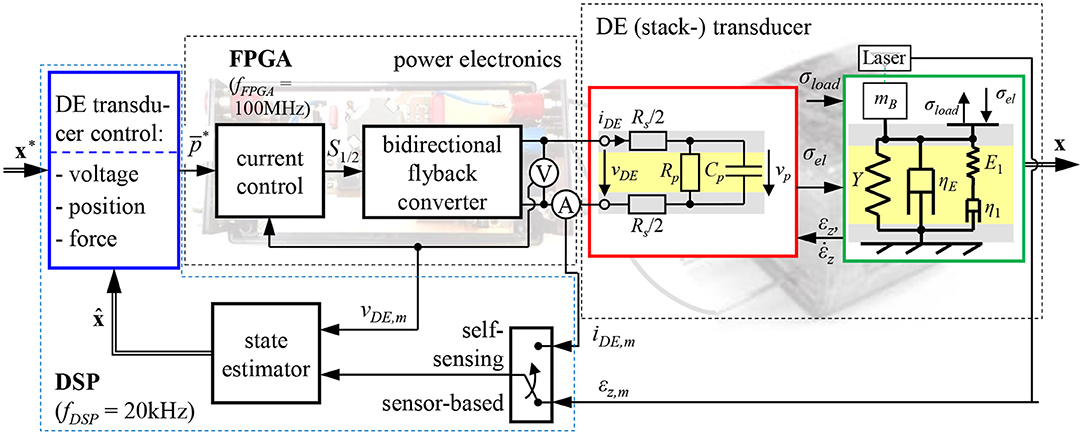
Figure 1. Fundamental structure of the proposed closed-loop position control for DE stack-actuators fed by a bidirectional flyback-converter.

As shown in the center and on the right hand side of Figure 1 the terminal voltage v_DE and current i_DE have to be measured to enable the combined actuator-sensor-operation. In order to determine the mechanical state based on these measurement quantities adequate self-sensing algorithms are required. Anderson et al. (2012) summarizes different approaches for this purpose. The goal of most self-sensing algorithms is to identify the capacitance of the DE transducer in a first step and afterwards estimate the deformation and force based on a model or experimentally obtained information about the deformation dependency of the capacitance. For almost all approaches the driving voltage v_DE is superimposed with a harmonic excitation that is used for the sensor functionality.

Chuc et al. (2008) and Jung et al. (2008) published first frequency domain based approaches by experimentally identifying changes of the electrical impedance of a DE transducer under deformation when it is excited by a harmonic voltage v_DE. Beside the capacitance C_p they also considered losses in the polymer and the electrode by adding the resistances R_s and R_p, respectively, see Figure 1.

In Hoffstadt et al. (2014) another model-based identification algorithm in the frequency domain is presented that estimates the electrical parameters of a DE transducer by evaluating the amplitudes of and the phase shift between the superimposed terminal voltage and current. Furthermore, it was shown that the behavior of a DE transducer can be sufficiently modeled by neglecting the parallel resistance R_p representing losses in the dielectric, if the DE transducer is excited with a comparable high frequency.

The extended Kalman-filter introduced in Hoffstadt and Maas (2018a) estimates the strain of a DE transducer without any superimposed excitation so that it can be used independent of the utilized power electronics. Other approaches in the time domain estimate the charge q_p of the capacitance C_p. Under further consideration of the measured voltage v_DE the capacitance C_p ≈ q_p/v_DE can be determined (Matysek et al., 2011; Gisby et al., 2013).

Rizzello et al. (2017) developed a self-sensing algorithm based on the recursive least squares (RLS) method. For this purpose, he takes into account the equivalent circuit diagram with three parameters (see Figure 1). In a first step, the parameters of a discrete transfer function describing the behavior of the considered circuit are estimated. As these parameters depend on the electrical parameters, they can be calculated afterwards. For the identification a harmonic excitation signal is superimposed.

Although several self-sensing approaches have been developed only a few closed-loop self-sensing controller designs have been published, so far. Gisby et al. (2011) controls the deformation of a single-layer circular DE transducer by using the already mentioned self-sensing approach (Gisby et al., 2013). Here, the terminal voltage is PWM generated. While the deformation of the DE transducer mainly depends on the mean of this voltage, the included higher harmonics are used to enable the sensor functionality. The manually adjusted proportional gain controller yields comparable low dynamics and accuracy. Therefore, Rosset et al. (2013) extends this controller to a PI-controller, using the same self-sensing approach (Gisby et al., 2013). Here, the parameters of the controller are optimized for one particular operating point of the nonlinear control plant. The derived controller is used to control an optical grid.

Rizzello et al. (2016) systematically combines his RLS-based self-sensing approach (Rizzello et al., 2017) with his robust position controller (Rizzello et al., 2015) to control the deformation of a DE membrane actuator. For the combined actuator-sensor-operation the required driving voltage determined by the controller is superimposed with a harmonic excitation with a high frequency of 1 kHz and an amplitude of 75 V. Compared to the sensor-based control (Rizzello et al., 2015) almost no drawbacks in terms of the accuracy are observed, while the bandwidth of the closed-loop self-sensing control is reduced due to the dynamics of the parameter identification.

Within the referenced publications costly and bulky high-voltage amplifiers were used to feed the DE transducer. However, due to the capacitive behavior of DE transducers voltage-fed current sources are well suited instead of high-voltage amplifiers (Eitzen et al., 2011a). Here, compact and efficient driving electronics can be realized when using switched-mode operated topologies like the bidirectional flyback converter. This converter allows not only to supply the DE transducer with a certain voltage but also to recover the energy stored in the DE transducer when discharging it.

Under consideration of the properties of the bidirectional flyback converter and the DE transducer, we previously published sensor-based position and force controls in Hoffstadt and Maas (2017, 2018b) that use the directly measured deformation as feedback-signal, cf. Figure 1. Within this publication we extend them to a self-sensing controller that is able to universally control the voltage, force or deformation of the DE transducer by just measuring the terminal voltage v_DE and current i_DE. For this purpose, in the following section 2 the considered control plant comprising a DE stack-transducer (Maas et al., 2015) fed by a bidirectional flyback converter (Eitzen et al., 2011b; Hoffstadt and Maas, 2016) is introduced and modeled. The design of the novel self-sensing state and disturbance estimator is presented in section 3. Due to the non-linear behavior of the control plant an extended Kalman-filter (EKF) is used for this purpose (Welch and Bishop, 2001). The developed estimator does not require any superimposed excitation. The subsequently presented controller design (Hoffstadt and Maas, 2017, 2018b) is based on the sliding mode control approach (DeCarlo et al., 1988) as this is well suited for the considered control plant and its characteristic behavior. The self-sensing estimator and control are experimentally validated in section 5. Finally, section 6 summarizes the developed approaches and the result.

2. Model of the DE Transducer System

Figure 2A shows a schematic representation of the considered DE stack-transducer with N layers. This multilayer design is used to scale the deformation Δz in z-direction, as one single layer has an initial thickness of only d₀ = 50 μm. Details about the design and the manufacturing were published by Maas et al. (2015). The static strain-force-behavior is shown in Figure 2B. The transducer generates higher tensile forces F_act at smaller strains ε_z = Δz/z₀, with z₀ = N · d₀. By increasing the initial electric field strength E₀ = v_DE/d₀ the electrostatic pressure according to Equation (1) increases so that higher forces and strains are obtained. The blocking-force F_act(ε_z = 0) and the no-load strain ε_z(F_act = 0) represent two characteristic points of the strain-force behavior.

FIGURE 2

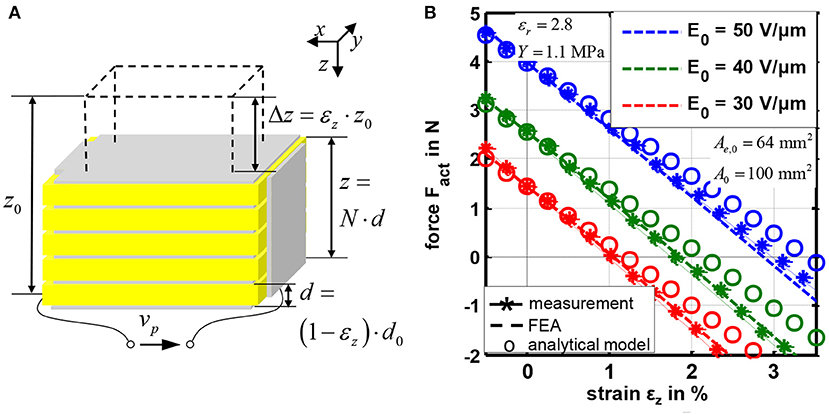
Figure 2. Schematic design (A) and static strain-force characteristics (B) of the considered silicone-based DE stack-actuators.

An analytical model for this transducer is published in Hoffstadt and Maas (2015). In Figure 2 the modeled results of the static strain-force behavior are compared with measurement results and a finite element analysis (FEA) published by Kuhring et al. (2015). The analytical model is based on the structure shown on the right of Figure 1. The actuator tension σ_act is given by the force equilibrium:

$\begin{array}{ll}{\sigma }_{\text{act}}=\beta ·{\sigma }_{\text{el}}-{\sigma }_{\text{elast}}-{\eta }_E·{\dot{\epsilon }}_z-E_1·{\epsilon }_{E_1},\text{ with }\beta =\frac{A_{\text{e}}}{A}.& (2)\end{array}$

Here, σ_elast is the elastic material tension that is calculated using the Neo-Hookean approach with the Young's modulus Y to consider the hyperelastic, non-linear material behavior:

$\begin{array}{ll}{\sigma }_{elast}=\frac{Y}{3}·\left(\frac{1}{1-{\epsilon }_z}-{\left(1-{\epsilon }_z\right)}^2\right).& (3)\end{array}$

Beside this reversible elastic behavior, viscoelastic properties are taken into account with the viscosity η_E and the Maxwell element with stiffness E₁ and viscosity η₁. Furthermore, with the area ratio β it is considered that the electrostatic pressure σ_el acts only on the area A_e covered with electrode, while all other tensions are assumed to homogeneously act on the whole transducer area A in z-direction. Instead of applying Equation (1) for the electrostatic pressure σ_el, here it is determined depending on the energy U_c,diel in the electric field of the capacitance C_p:

$\begin{array}{ll}\beta ·{\sigma }_{\text{el}}=\frac{2}{V}·U_{\text{c},\text{diel}}.& (4)\end{array}$

The bidirectional flyback converter control proposed in Hoffstadt and Maas (2016) enables three discrete input states in terms of the feeding power $\bar{p}$. Beside an off-state, the DE can be charged and discharged with almost constant power depending on the characteristic energy increment ΔU_max transfered during every switching period T_S of the converter:

$\begin{array}{l}\overline{p}=\{\begin{array}{l}+{\overline{p}}_{\max }=+\frac{\Delta U_{\max }}{T_{\text{S}}},\text{ charging}\hfill \\ 0,\text{ off-state}\hfill \\ -{\overline{p}}_{\max }=-\frac{\Delta U_{\max }}{T_{\text{S}}},\text{ discharging}\hfill \end{array}\\ \text{with }\Delta U_{\max }=\frac{1}{2}·L_{\text{m}}·I_{\text{m},\max }.& (5)\end{array}$

The energy increment ΔU_max depends on the magnetizing inductance L_m of the converter and the magnetizing current I_m,max adjusted by its inner control. Under further consideration of losses p_Re dissipated in the electrode material the power ${\bar{p}}^{\prime }=\bar{p}-p_{Re}$ feeds the capacitance of the DE transducer. With this, the electromechanically coupled behavior of a DE transducer can be modeled based on a power balance yielding the state space representation

$\begin{array}{l}\dot{x}=\left[\begin{array}{c}{\dot{\epsilon }}_z\\ \frac{V}{m_{\text{B}}·z_0^2}·\frac{{\sigma }_{\text{act}}-{\sigma }_{\text{load}}}{1-{\epsilon }_z}\\ {\dot{\epsilon }}_z-\frac{E_1}{{\eta }_1}·{\epsilon }_{E_1}\\ -2·U_{\text{c},\text{diel}}·\left(\frac{{\dot{\epsilon }}_z}{1-{\epsilon }_z}+\frac{1}{{\tau }_{\text{p}}}\right)\end{array}\right]+\left[\begin{array}{c}0\\ 0\\ 0\\ 1\end{array}\right]·{\overline{p}}^{\prime },\\ \text{with }x=\left[\begin{array}{c}{\epsilon }_z\\ {\dot{\epsilon }}_z\\ {\epsilon }_{E_1}\\ U_{\text{c},\text{diel}}\end{array}\right].& (6)\end{array}$

Beside the strain ε_z and the energy U_c,diel the state vector x includes the velocity ${\dot{\epsilon }}_z$ as well as the strain ε_E1 of the stiffness E₁ of the Maxwell element. Depending on the supplied input power ${\bar{p}}^{\prime }$ and an external load σ_load the inner states of the DE transducer with volume V and accelerated mass m_B can be calculated with Equation (6).

For the subsequently developed self-sensing state estimator models describing the strain dependency of the electrical transducer parameters are required, too. The series resistance R_s mainly comprises losses in the contacting of the DE transducer and electrodes that are applied on the initial area A_{e, 0} of every layer. It was shown Hoffstadt et al. (2016) that this resistance is almost constant in the relevant range of deformation. In contrast, the capacitance C_p for the N layers connected in parallel is given by:

$\begin{array}{ll}{C}_{\text{p}}=N·{\epsilon }_0·{\epsilon }_{\text{r}}·\frac{A_{\text{e},\text{0}}}{d_0}·\frac{1}{{\left(1-{\epsilon }_z\right)}^{\kappa }}=C_{\text{p},\text{0}}·\frac{1}{{\left(1-{\epsilon }_z\right)}^{\kappa }}& (7)\end{array}$

The change of the initial capacitance C_{p, 0} also depends on the factor κ. In case of an absolutely homogeneous deformation without constraints, κ = 2 would apply. However, due to a passive area around A_e that is required for insulation purposes, as well as due to stiff mechanical interfaces applied on the top and/or bottom of the transducer, here the factor is slightly decreased to κ = 1.85.

In analogy, the strain dependency of the parallel resistance R_p reads as follows:

$\begin{array}{ll}{R}_{\text{p}}=\frac{1}{N}·{\rho }_{\text{p}}·\frac{d_0}{A_{\text{e},\text{0}}}·{\left(1-{\epsilon }_z\right)}^{\kappa }=R_{\text{p},\text{0}}·{\left(1-{\epsilon }_z\right)}^{\kappa }.& (8)\end{array}$

This resistance represents losses in the dielectric with the specific resistance ϱ_p.

Although C_p and R_p vary with the strain ε_z the resulting time constant τ_p is independent of the strain:

$\begin{array}{ll}{\tau }_{\text{p}}=R_{\text{p}}·C_{\text{p}}={\epsilon }_0·{\epsilon }_{\text{r}}·{\rho }_{\text{p}}=\text{const.}& (9)\end{array}$

3. EKF-Based Self-Sensing Algorithm

In Hoffstadt and Maas (2018a) we already published a self-sensing estimator based on a discrete, extended Kalman-filter that estimates the strain of the DE transducer without superimposed excitation. However, for the closed-loop operation beside the inner states of the transducer also the disturbance σ_load has to be estimated. For example, this load tension might result from a collision of an external device or human with a soft-bodied robot equipped with DE transducers. Therefore, a new and extended approach based on Equation (6) is applied here. As mentioned above, the goal is to determine the electromechanical state of the DE transducer based on the measured terminal voltage v_DE and the current i_DE. However, in Equation (6) the energy U_c,diel represents the electrical state. Therefore, a modification of the model is required to design the self-sensing estimator.

For this purpose, the change of the charge q_p on the capacitance C_p is taken into account. It can be calculated under consideration of the current i_DE and the leakage current v_p/R_p = q_p/τ_p, see Figure 1:

$\begin{array}{ll}{\dot{q}}_{\text{p}}=i_{\text{DE}}-\frac{v_{\text{p}}}{R_{\text{p}}}=i_{\text{DE}}-\frac{1}{{\tau }_{\text{p}}}·q_{\text{p}},\text{ with }{q}_{\text{p}}=C_{\text{p}}·v_{\text{p}}.& (10)\end{array}$

As the charge depends on the measured current and the invariant time constant τ_p from Equation (9), it is used as input variable u_qv in the following. Furthermore, if instead of the energy U_c,diel the charge q_p is considered, the electrostatic pressure can be expressed by:

$\begin{array}{ll}\beta ·{\sigma }_{\text{el}}=\frac{2}{V}·U_{\text{c},\text{diel}}=\frac{q_{\text{p}}^2}{V·C_{\text{p}}\left({\epsilon }_z\right)},\text{ with }{U}_{\text{c},\text{diel}}=\frac{1}{2}·\frac{q_{\text{p}}^2}{C_{\text{p}}\left({\epsilon }_z\right)}.& (11)\end{array}$

Additionally, the voltage v_p across C_p depends on the terminal voltage v_DE reduced by the voltage drop R_s · i_DE across the series resistance R_s that is assumed to be constant here:

$\begin{array}{ll}{v}_{\text{p}}=\frac{q_{\text{p}}}{C_{\text{p}}\left({\epsilon }_z\right)}=v_{\text{DE}}-R_{\text{s}}·i_{\text{DE}}.& (12)\end{array}$

This voltage will be used as output variable y_qv afterwards.

Beside the mechanical states included in x and Equation (6) the external load σ_load has to be estimated as disturbance, too. As it represents an unknown disturbance it is assumed (according to Isermann and Munchhof, 2011) that it is constant during one sample time T of the discrete EKF implemented on a DSP. By applying ${\dot{\sigma }}_{\text{load}}=0$ in combination with Equations (10)–(12) a fourth order system can be established for the estimation:

$\begin{array}{l}{x}_{qv}^{\cdot }=f_{qv}\left(x_{qv},u_{qv}\right)=\left[\begin{array}{c}{\dot{\epsilon }}_z\\ {\gamma }_1·\frac{{\sigma }_{\text{act}}\left(q_p\right)-{\sigma }_{\text{load}}}{1-{\epsilon }_z}\\ {\dot{\epsilon }}_z-\frac{E_1}{{\eta }_1}·{\epsilon }_{E_1}\\ 0\end{array}\right],\\ \text{ with }{x}_{qv}=\left[\begin{array}{c}{\epsilon }_z\\ {\epsilon }_z\\ {\epsilon }_{E_1}\\ {\sigma }_{\text{load}}\end{array}\right],{\gamma }_1=\frac{V}{m_{\text{B}}·z_0^2}\text{ and}\\ y_{qv}=g_{qv}\left(x_{qv},u_{qv}\right)=\frac{{\left(1-{\epsilon }_z\right)}^{\kappa }}{C_{\text{p},\text{0}}}·q_{\text{p}}=v_{\text{p}}=v_{\text{DE},\text{m}}-R_{\text{s}}·i_{\text{DE},\text{m}}.& (13)\end{array}$

According to Adamy (2014) the observability of the nonlinear system (13) is given if the determinant of the observability matrix Q_B,qv is not zero. This matrix can be calculated under consideration of the Lie derivatives $L_{f_{qv}}^i{g}_{qv}$, with i = 0, …, 3:

$\begin{array}{ll}{Q}_{\text{B},qv}\left(x_{qv},u_{qv}\right)=\left[\begin{array}{c}\frac{\partial L_{f_{qv}}^0{g}_{qv}\left(x_{qv},u_{qv}\right)}{\partial x_{qv}}\\ \frac{\partial L_{f_{qv}}^1{g}_{qv}\left(x_{qv},u_{qv}\right)}{\partial x_{qv}}\\ \frac{\partial L_{f_{qv}}^2{g}_{qv}\left(x_{qv},u_{qv}\right)}{\partial x_{qv}}\\ \frac{\partial L_{f_{qv}}^3{g}_{qv}\left(x_{qv},u_{qv}\right)}{\partial x_{qv}}\end{array}\right]=\left[\begin{array}{c}\frac{\partial g_{qv}\left(x_{qv},u_{qv}\right)}{\partial x_{qv}}\\ \frac{\partial L_{f_{qv}}^1{g}_{qv}\left(x_{qv},u_{qv}\right)}{\partial x_{qv}}\\ \frac{\partial L_{f_{qv}}^2{g}_{qv}\left(x_{qv},u_{qv}\right)}{\partial x_{qv}}\\ \frac{\partial L_{f_{qv}}^3{g}_{qv}\left(x_{qv},u_{qv}\right)}{\partial x_{qv}}\end{array}\right]& (14)\end{array}$

Beside material parameters that are different from zero, the determinant of Q_B,qv depends on the charge q_p and the strain ε_z:

$\begin{array}{l}\det \left(Q_{\text{B},qv}\left(x_{qv},u_{qv}\right)\right)=q_{\text{p}}^4·\frac{{\gamma }_1^2·{\kappa }^4·E_1^2}{{\eta }_1·C_{\text{p}}^4\left({\epsilon }_z\right)·{\left(1-{\epsilon }_z\right)}^6}\ne 0,\\ \text{ for }{\epsilon }_z<1\text{ and }{q}_{\text{p}}\ne 0.& (15)\end{array}$

The strain ε_z is always smaller than one, and thus does not influence the observability. However, the uncharged state with q_p = 0 is not observable. In contrast for example to piezoelectric materials, this is due to the fact that the DE materials do not contain inherent dipoles causing a charge separation under deformation. Instead, a DE transducer has to be electrically pre-charged so that a current flow or change of voltage can be detected when it is deformed. Furthermore, the restricted observability for q_p = 0 is not only a drawback of the proposed approach. All referenced self-sensing methods have the same issue, but the usually superimposed voltage excitations ensure that this operating point does not occur. As this superimposed excitation is not required for the EKF-based estimator a certain amount of charge q_p,min is always applied, here.

This results in the structure of the EKF-based self-sensing state and disturbance estimator shown in Figure 3. As the EKF will be implemented on a DSP its discrete implementation according to Welch and Bishop (2001) is applied. Using the external estimation of the charge by filtering the measured current i_DE,m has the advantage, that the state vector x_qv only includes mechanical states that have to be estimated with the EKF. Furthermore, the parameterization effort increases significantly with increasing system order so that it is meaningful to use a system with order n = 4 instead of n = 5.

FIGURE 3

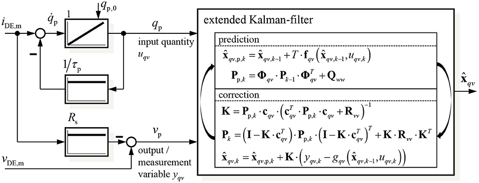
Figure 3. Structure of the proposed self-sensing state and disturbance estimator based on an extended Kalman-filter.

For the implementation of the Kalman-filter algorithm according to Figure 3 the system (13) has to be linearized in the predicted state ${\widehat{x}}_{qv,\text{p},k}$:

$\begin{array}{l}{A}_{qv,k}={\frac{\partial f_{qv}\left(x_{qv},u_{qv}\right)}{\partial x_{qv}}|}_{{\widehat{x}}_{qv,\text{p},k},u_{qv,k}}\\ =\left[\begin{array}{cccc}0& 1& 0& 0\\ a_{qv,21}& \frac{-{\gamma }_1·{\eta }_{\text{E}}}{1-{\widehat{\epsilon }}_{z,\text{p}}}& \frac{-{\gamma }_1·E_1}{1-{\widehat{\epsilon }}_{z,\text{p}}}& \frac{-{\gamma }_1}{1-{\widehat{\epsilon }}_{z,\text{p}}}\\ 0& 1& -\frac{E_1}{{\eta }_1}& 0\\ 0& 0& 0& 0\end{array}\right],\\ \text{with }{a}_{qv,21}=\frac{{\gamma }_1}{1-{\widehat{\epsilon }}_{z,\text{p}}}·\left[\frac{{\widehat{\sigma }}_{\text{act},\text{p}}\left(u_{qv,k}\right)-{\widehat{\sigma }}_{\text{load},\text{p}}}{1-{\widehat{\epsilon }}_{z,\text{p}}}-\frac{d{\widehat{\sigma }}_{\text{elast},\text{p}}}{d{\widehat{\epsilon }}_{z,\text{p}}}-\frac{d{\widehat{\sigma }}_{\text{el},\text{p}}}{d{\widehat{\epsilon }}_{z,\text{p}}}\right],\\ \text{and }\frac{d{\widehat{\sigma }}_{\text{el},\text{p}}}{d{\widehat{\epsilon }}_{z,\text{p}}}\underset{\left(7\right)}{\overset{\left(11\right)}{=}}-\frac{\kappa ·q_{\text{p}}^2·{\left(1-{\widehat{\epsilon }}_{z,\text{p}}\right)}^{\kappa -1}}{V·C_{\text{p},0}}.& (16)\end{array}$

Based on this the discrete transition matrix Φ_qv can be approximated by (Ifeachor and Jervis, 2002):

$\begin{array}{ll}{\Phi }_{qv}\approx I+A_{qv,k}·T,& (17)\end{array}$

where I represents the unity matrix of order n = 4. The output vector $c_{qv,k}^T$ is calculated by the jacobian of the output function g_qv in Equation (13) with respect to the state vector x_qv:

$\begin{array}{l}{c}_{qv,k}^T={\frac{\partial g_{qv}\left(x_{qv},u_{qv}\right)}{\partial x_{qv}}|}_{{\widehat{x}}_{qv,rmp,k},u_{qv,k}}\\ =\left[-\frac{\kappa ·{\left(1-{\widehat{\epsilon }}_{z,p}\right)}^{\kappa -1}}{C_{\text{p},\text{0}}}·u_{qv,k}000\right].& (18)\end{array}$

With these information the predicted state ${\widehat{\text{x}}}_{qv,\text{p},k}$ and the related covariance matrix P_p,k can be determined in the prediction step (denoted by the index p) of the algorithm shown in Figure 3. In the following correction the Kalman matrix K and covariance matrix P_k are calculated to update the estimated state vector ${\widehat{\text{x}}}_{qv,k}$. The covariance matrices of the measurement and system noise R_vv and Q_ww, respectively, will be parameterized in the validation section 5. With the information, included in the state vector x_qv,k and Equation (4) to calculate the energy U_c,diel based on the charge q_p, all state variables in x from Equation (6) as well as the load σ_load can be determined.

4. Self-Sensing Sliding Mode Control

The considered control plant modeled with Equation (6) has a strongly non-linear behavior. Furthermore, the bidirectional flyback converter allows to supply discrete feeding powers $\bar{p}$ so that it can be described by the three-point switch in Equation (5). Due to these properties the design of a variable structure control is well suited. In Hoffstadt and Maas (2017) a position controller based on the model (6) was introduced that uses the sliding mode control (SMC), for this purpose. Additionally, a SMC force controller was published in Hoffstadt and Maas (2018b). In the following it will be shown that this controller cannot be used to solely control the force F_act of the DE transducer but also the strain ε_z and the voltage v_p by applying different feed-forward structures to one and the same controller. This flexibility makes the approach advantageous for sophisticated applications like in soft robotics. The detailed design of the controller shown in Figure 4 can be found in Hoffstadt and Maas (2018b) and will be summarized in the following.

FIGURE 4

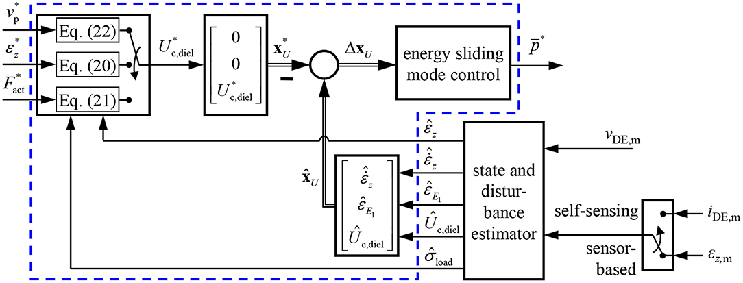
Figure 4. Detailed structure of the controller (blue box in Figure 1) including a feed-forward structure to either control the voltage, strain or force and a three-point controller with hysteresis and adaption of the inner flyback converter control.

In case of the SMC a static setpoint state vector x^* has to be defined including setpoints for every state variable. Under consideration of the static force equilibrium

$\begin{array}{ll}\underset{t\to \infty }{\lim }{\sigma }_{\text{act}}\left(t\right)=\beta ·{\sigma }_{\text{el}}-{\sigma }_{\text{elast}}\stackrel{\left(4\right)}{=}\frac{2}{V}·U_{\text{c},\text{diel}}-{\sigma }_{\text{elast}}\stackrel{!}{=}{\sigma }_{\text{load}}& (19)\end{array}$

resulting from Equation (2) setpoints for the energy $U_{\text{c},\text{diel}}^{*}$ can be derived. On the one hand, the energy can be calculated depending on a setpoint strain ${\epsilon }_z^{*}$:

$\begin{array}{ll}{U}_{\text{c},\text{diel}}^{*}\left({\epsilon }_z^{*}\right)=\frac{V}{2}·\left({\sigma }_{\text{elast}}\left({\epsilon }_z^{*}\right)+{\sigma }_{\text{load}}\right).& (20)\end{array}$

To achieve this strain the electrostatic pressure caused by the energy according to Equation (4) has to compensate the elastic material tension ${\sigma }_{\text{elast}}({\epsilon }_z^{*})$ given by Equation (3) as well as the influence of the disturbance σ_load. On the other hand, if the DE transducer should generate a certain force $F_{\text{act}}^{*}=A·{\sigma }_{\text{act}}$ the corresponding energy $U_{\text{c},\text{diel}}^{*}$ is given by:

$\begin{array}{l}{U}_{\text{c},\text{diel}}^{*}\left(F_{\text{act}}^{*}\right)=\frac{V}{2}·\left(\frac{F_{\text{act}}^{*}}{A\left({\epsilon }_z\right)}+{\sigma }_{\text{elast}}\left({\epsilon }_z\right)\right),\\ \text{ with }{\sigma }_{\text{load}}=\frac{F_{\text{act}}^{*}}{A\left({\epsilon }_z\right)}\text{and }A\left({\epsilon }_z\right)=\frac{A_0}{1-{\epsilon }_z}.& (21)\end{array}$

In this case, the influence of the elastic deformation has to be compensated, i.e., the energy has to be increased with increasing strain ε_z (see Figure 2B).

Beside these approaches, the energy $U_{\text{c},\text{diel}}^{*}$ can be also determined depending on a setpoint voltage $v_{\text{p}}^{*}$ across the capacitance C_p(ε_z) in Equation (7):

$\begin{array}{ll}{U}_{\text{c},\text{diel}}^{*}\left(v_{\text{p}}^{*}\right)=\frac{1}{2}·C_{\text{p}}\left({\epsilon }_z\right)·v_{\text{p}}^{*}{}^2.& (22)\end{array}$

With Equations (20)–(22) three approaches exist to define a setpoint value for the energy $U_{\text{c},\text{diel}}^{*}$. For the system (6) also a setpoint for the strain ${\epsilon }_z^{*}$ is required, while the other two state variables are zero during steady state ${\dot{\epsilon }}_z={\epsilon }_{E_1}=0$, respectively. However, especially if the force or voltage should be controlled by applying Equations (21) or (22), they should be independent of the strain, i.e., that no setpoint ${\epsilon }_z^{*}$ can be defined in this case. To overcome this issue, the control design is based on a reduced system (23) with ${\dot{\epsilon }}_z$, ε_E1 and U_c,diel as state variables while the strain ε_z together with the load tension σ_load is considered to be a disturbance, here:

$\begin{array}{l}{\dot{x}}_U=\left[\begin{array}{c}{\ddot{\epsilon }}_z\\ {\dot{\epsilon }}_{E_1}\\ {\dot{U}}_{\text{c},\text{diel}}\end{array}\right]=\underset{f_U\left(x_U,z\right)}{\underbrace{\left[\begin{array}{c}\frac{V}{m_{\text{B}}·z_0^2}·\frac{{\sigma }_{\text{act}}-{\sigma }_{\text{load}}}{1-{\epsilon }_z}\\ {\dot{\epsilon }}_z-\frac{E_1}{{\eta }_1}·{\epsilon }_{E_1}\\ -2·U_{\text{c},\text{diel}}·\left(\frac{{\dot{\epsilon }}_z}{1-{\epsilon }_z}+\frac{1}{{\tau }_{\text{p}}}\right)\end{array}\right]}}+\underset{b_U}{\underbrace{\left[\begin{array}{c}0\\ 0\\ 1\end{array}\right]}}·{\overline{p}}^{\prime },\\ \text{with }z=\left[\begin{array}{c}{\epsilon }_z\\ {\sigma }_{\text{load}}\end{array}\right]·& (23)\end{array}$

In this case, the setpoint state vector reads as:

$\begin{array}{ll}{\dot{x}}_U^{\ast }={\left[\begin{array}{ccc}0& 0& U_{\text{c},\text{diel}}^{*}\end{array}\right]}^T.& (24)\end{array}$

4.1. Design of the Sliding Mode

The control operation with a SMC is characterized by two phases. During the sliding mode the system is led toward its setpoint x^* on the switching function S(Δx) = S(x − x^*) = 0. Within the reaching phase it is ensured, first, that this switching function is reached from any arbitrary initial state. According to DeCarlo et al. (1988) one comparable simple approach for the design of the switching function is obtained if the system is in standard canonical form (denoted by the index R). To determine a corresponding transformation matrix T, the system (23) has to be linearized yielding the system matrix A_U for the estimated state ${\widehat{\text{x}}}_U$:

$\begin{array}{ll}{A}_U={\frac{\partial f_U\left(x_U,z\right)}{\partial x_U}|}_{x_U={\widehat{x}}_U}=\left[\begin{array}{ccc}\frac{-{\gamma }_1·{\eta }_{\text{E}}}{1-{\widehat{\epsilon }}_z}& \frac{-{\gamma }_1·E_1}{1-{\widehat{\epsilon }}_z}& \frac{{\gamma }_1·2/V}{1-{\widehat{\epsilon }}_z}\\ 1& -\frac{E_1}{{\eta }_1}& 0\\ -\frac{2·{\widehat{U}}_{\text{c},\text{diel}}}{1-{\widehat{\epsilon }}_z}& 0& -\frac{2·{\widehat{\dot{\epsilon }}}_z}{1-{\widehat{\epsilon }}_z}-\frac{2}{{\tau }_{\text{p}}}\end{array}\right].& (25)\end{array}$

As the system behaves linear concerning the input u, the constant input vector b_U is already given in Equation (23). With these information the following transformation matrix T can be derived as proposed by Kalman (1960):

$\begin{array}{l}T=-\frac{V}{2}·\frac{1-{\widehat{\epsilon }}_z}{{\gamma }_1}·\left[\begin{array}{ccc}0& -1& 0\\ -1& \frac{E_1}{{\eta }_1}& 0\\ t_{31}& t_{32}& -\frac{2}{V}·\frac{{\gamma }_1}{1-{\widehat{\epsilon }}_z}\end{array}\right]\\ \text{with }{t}_{31}=\frac{E_1}{{\eta }_1}+\frac{{\gamma }_1·{\eta }_E}{1-{\widehat{\epsilon }}_z}\text{ and }{t}_{32}=\frac{E_1}{{\eta }_1}·\left(\frac{{\gamma }_1·{\eta }_1}{1-{\widehat{\epsilon }}_z}-\frac{E_1}{{\eta }_1}\right).& (26)\end{array}$

For the considered single input single output (SISO) system a linear switching function is defined:

$\begin{array}{l}S\left(\Delta x_{\text{R}}\right)=c^T·\Delta x_{\text{R},U}=\left[\begin{array}{ccc}{c}_1& c_2& c_3\end{array}\right]·T·\left({\widehat{x}}_U-x_U^{\ast }\right),\\ \text{ with }\Delta x_{\text{R},U}=T·\left({\widehat{x}}_U-x_U^{\ast }\right).& (27)\end{array}$

During the sliding mode S(Δx_R) = 0 as well as Ṡ(Δx_R) = 0 applies. This behavior is obtained by the equivalent input (DeCarlo et al., 1988)

$\begin{array}{l}{u}_{\text{eq}}=-{\left(c^T·b_{\text{R},U}\right)}^{-1}·c^T·A_{\text{R},U}·\Delta x_{\text{R},U},\\ \text{ with }{A}_{\text{R},U}=T·A_U·T^{-1}\text{ and }{b}_{\text{R},U}=T·b_U.& (28)\end{array}$

With this input the dynamics during the sliding mode only depend on the coefficients c_i, with i = 1, 2, 3, of the switching function in Equation (27):

$\begin{array}{l}\Delta {\dot{x}}_{\text{R},U}=A_{\text{R},U}·\Delta x_{\text{R},U}+b_{\text{R},U}·u_{\text{eq}}\\ =\left[I-b·{\left[c^T·b\right]}^{-1}·c^T\right]·A_{\text{R},U}·\Delta x_{\text{R},U}\\ =\left[\begin{array}{ccc}0& 0& 0\\ 0& 0& 1\\ 0& -\frac{c_1}{c_3}& -\frac{c_2}{c_3}\end{array}\right]·\Delta x_{\text{R}}=\left[\begin{array}{cc}0& 0^T\\ 0& {\tilde{A}}_1\end{array}\right]·\Delta x_{\text{R},U}.& (29)\end{array}$

An other characteristic property of the SMC approach is that during the sliding mode the system order n is reduced by the number of inputs p (here p = 1). Thus, the dynamics during the sliding mode can be defined by a pole placement under consideration of ${\tilde{A}}_1$. For a second order element with damping coefficient D and cut-off frequency ω_g this results in:

$\begin{array}{l}\det \left(s·I-{\tilde{A}}_{1,U}\right)=s^2+\frac{c_2}{c_3}·s+\frac{c_1}{c_3}\stackrel{!}{=}{s}^2+2·D·{\omega }_{\text{g}}·s+{\omega }_{\text{g}}^2\\ \text{ with }{c}_3=1,\Rightarrow c_1={\omega }_{\text{g}}^2,c_2=2·D·{\omega }_{\text{g}}.& (30)\end{array}$

4.2. Reachability

To reach this sliding mode a proper controller function u(Δx_R,U) has to be determined and parametrized under consideration of the properties of the feeding power electronics. One approach to prove the reachability is based on an investigation of the Laypunov function $V(\Delta x_{\text{R},U})=1/2·S^2(\Delta x_{\text{R},U})$. To ensure stable steady-state behavior the time derivate of the Lyapunov function has to be negative:

$\begin{array}{ll}\dot{V}\left(\Delta x_{\text{R},U}\right)=S\left(\Delta x_{\text{R},U}\right)·\dot{S}\left(\Delta x_{\text{R},U}\right)\stackrel{!}{<}0.& (31)\end{array}$

The derivative of the switching function is given by:

$\begin{array}{l}\dot{S}\left(\Delta x_{\text{R},U}\right)=c^T·T·\left(A_U·\Delta x_U+b_U·u\left(\Delta x_{\text{R},U}\right)\right)\\ ={\zeta }_1·\Delta {\dot{\epsilon }}_z+{\zeta }_2·\Delta {\epsilon }_{E1}+{\zeta }_3·\Delta U_{\text{c},\text{diel}}+u\left(\Delta x_{\text{R},U}\right),\text{ with}& (32)\end{array}$

$\begin{array}{l}{\zeta }_1=\frac{V}{2·{\gamma }_1}({\omega }_{\text{g}}^2-2·D·{\omega }_{\text{g}}·\left({\gamma }_1·{\eta }_{\text{E}}+\frac{E_1}{{\eta }_1}\right)\\ +{\gamma }_1^2·{\eta }_{\text{E}}^2+{\gamma }_1·E_1·\left(\frac{{\eta }_{\text{E}}}{{\eta }_1}-1\right)+\frac{E_1^2}{{\eta }_1^2}),& (\mathrm{33a})\end{array}$

$\begin{array}{l}{\zeta }_2=\frac{V·E_1}{2·{\gamma }_1·{\eta }_1}·({\omega }_{\text{g}}^2+2·D·{\omega }_{\text{g}}·\left({\gamma }_1·{\eta }_1-\frac{E_1}{{\eta }_1}\right)\\ -2·{\gamma }_1·E_1-{\gamma }_1^2·{\eta }_{\text{E}}·{\eta }_1+\frac{E_1^2}{{\eta }_1^2})\text{ and}& (\mathrm{33b})\end{array}$

$\begin{array}{ll}{\zeta }_3=2·D·{\omega }_{\text{g}}-\frac{2}{{\tau }_{\text{p}}}-\frac{E_1}{{\eta }_1}-{\gamma }_1·{\eta }_{\text{E}},\text{ for }{\widehat{x}}_U=0.& (\mathrm{33c})\end{array}$

The coefficients ζ₁, ζ₂ and ζ₃ depend on material parameters as well as the damping ratio D and cut-off frequency ω_g. These two controller parameters are chosen in such a way that the influence of the state variables $\Delta {\dot{\epsilon }}_z$ and Δε_E1 on Equation (32) vanishes. By solving ζ₁ = 0 and ζ₂ = 0 the following parameters result:

$\begin{array}{ll}{\omega }_{\text{g},0}=\sqrt{{\gamma }_1·E_1·\frac{{\eta }_1+{\eta }_{\text{E}}}{{\eta }_1}}\text{and}& (\mathrm{34a})\end{array}$

$\begin{array}{ll}{D}_0=\frac{1}{2}·\sqrt{\frac{{\left(E_1+{\gamma }_1·{\eta }_1·{\eta }_{\text{E}}\right)}^2}{{\gamma }_1·E_1·{\eta }_1·\left({\eta }_1+{\eta }_{\text{E}}\right)}}.& (\mathrm{34b})\end{array}$

According to Equation (5) the input power $\bar{p}$ supplied by the bidirectional flyback converter can be described by a three-point controller. However, for the design of the SMC the off-state with $\bar{p}=0$ can be neglected in a first step. Under consideration $\bar{p}=\pm {\bar{p}}_{max}$ a two-point controller is defined:

$\begin{array}{ll}u\left(\Delta x_{\text{R},U}\right)=\text{sgn}\left(S\left(\Delta x_{\text{R},U}\right)\right)·\varrho .& (35)\end{array}$

The parameter $\varrho =\pm {\bar{p}}_{max}$ will be chosen so that the reachability is ensured.

By inserting Equations (34), (34b), and (35) into Equation (32) the time derivative of the switching function simplifies to:

$\begin{array}{l}\dot{S}\left(\Delta x_{\text{R},U}\right)=-\frac{2}{{\tau }_{\text{p}}}·\Delta U_{\text{c},\text{diel}}+u\left(\Delta x_{\text{R},U}\right)\\ =\frac{2}{{\tau }_{\text{p}}}·U_{\text{c},\text{diel}}^{*}+\text{sgn}\left(S\left(\Delta x_{\text{R},\epsilon }\right)\right)·\varrho .& (36)\end{array}$

The control parameter ϱ is determined by applying a case-by-case analysis to satisfy Equation (31):

$\begin{array}{l}\text{I.: }S\left(\Delta x_{\text{R},U}\right)>0,\Rightarrow u\left(\Delta x_{\text{R},U}\right)=+\varrho ,\\ \Rightarrow \dot{S}\left(\Delta x_{\text{R},U}\right)=\frac{2}{{\tau }_{\text{p}}}·U_{\text{c},\text{diel}}^{*}+\varrho \stackrel{!}{<}0,\\ \text{II.: }S\left(\Delta x_{\text{R},U}\right)<0,\Rightarrow u\left(\Delta x_{\text{R},U}\right)=-\varrho ,\\ \Rightarrow \dot{S}\left(\Delta x_{\text{R},U}\right)=\frac{2}{{\tau }_{\text{p}}}·U_{\text{c},\text{diel}}^{*}-\varrho \stackrel{!}{>}0.& (37)\end{array}$

As the energy $U_{\text{c},\text{diel}}^{*}$ will always be equal to or larger than zero, both inequalities are solved by choosing:

$\begin{array}{ll}\varrho =-{{\overline{p}}^{\prime }}_{\max }\Rightarrow {{\overline{p}}^{\prime }}_{\max }>\frac{2}{{\tau }_{\text{p}}}·U_{\text{c},\text{diel}}^{*}.& (38)\end{array}$

Especially during steady state the introduced two-point controller will permanently switch between the positive and negative input power $\pm {\bar{p}}_{max}$. To avoid this chattering, the controller is extended to a three-point controller with hysteresis, as already shown in Figure 4:

$\begin{array}{ll}{\overline{p}}^{*}=\{\begin{array}{cc}+{\overline{p}}_{\max },& \begin{array}{c}\text{for }S\left(\Delta x_{\text{R},U}\right)\le -{\delta }_S\text{ or}-{\delta }_S<S\left(\Delta x_{\text{R},U}\right)<0\wedge \dot{S}\left(\Delta x_{\text{R},U}\right)>0\end{array}\\ 0,& \text{else}\\ -{\overline{p}}_{\max }& \begin{array}{c}\text{for }S\left(\Delta x_{\text{R},U}\right)\ge {\delta }_S\text{ or}0<S\left(\Delta x_{\text{R},U}\right)<{\delta }_S\wedge \dot{S}\left(\Delta x_{\text{R},U}\right)<0\end{array}\end{array}.& (39)\end{array}$

On the one hand, the off-state of the flyback converter is now taken into account, while on the other hand the hysteresis with threshold δ_S will significantly reduce the switching frequency in closed-loop operation. In Figure 4 an output limitation is also depicted that switches off the control, when the energy Û_c,diel exceeds a maximum value U_c,diel,max. Furthermore, to improve the steady state behavior the inner control of the flyback converter is adapted. Depending on the absolute value of the switching function |S(Δx_R,U)|, the maximum magnetizing current $I_{m,max}^{*}$ and thus the feeding power $\bar{p}$ according to Equation (5) is varied. This ensures, that for large control deviations corresponding to large values of |S(Δx_R,U)| the maximum feeding power is supplied for achieving the maximum dynamics. In contrast, for small control deviations the power is reduced for a higher accuracy by also adapting the hysteresis threshold δ_S. Further details can be found in Hoffstadt and Maas (2017, 2018b).

5. Experimental Validation

5.1. Test Setup for the Experimental Validation

Figure 5 schematically depicts the test setup used for the experimental validation of the self-sensing estimator and the self-sensing control. It consists of a bidirectional flyback converter that supplies the DE transducer with voltages up to 2.5 kV (Hoffstadt and Maas, 2016). The voltage v_DE,m is measured with the voltage probe TT-SI 9010 from Testec, while the current i_DE,m is determined by the voltage drop across the shunt resistance R_is = 1 kΩ. Details about the utilized DE transducers can be found in Maas et al. (2015). If no-load scenarios are investigated in the following, the displacement of the DE transducer is directly measured with the laser sensor OptoNCDT ILD 2300 from Micro-Epsilon. To apply loads to the DE transducer the test rig on the right hand side of Figure 5 will be used. It consists of a force measurement with the force sensor 9217A from Kistler and a voice coil linear drive VM8054-630 from Geeplus. The DE transducer can be attached between the force measurement and the linear drive. Via the voice coil load profiles with high dynamics can be applied to the DE transducer, while the resulting actuator force F_act,m is measured. Here, the same laser sensor as for the no-load scenarios measures the displacement of the rigidly coupled voice coil and DE transducer.

FIGURE 5

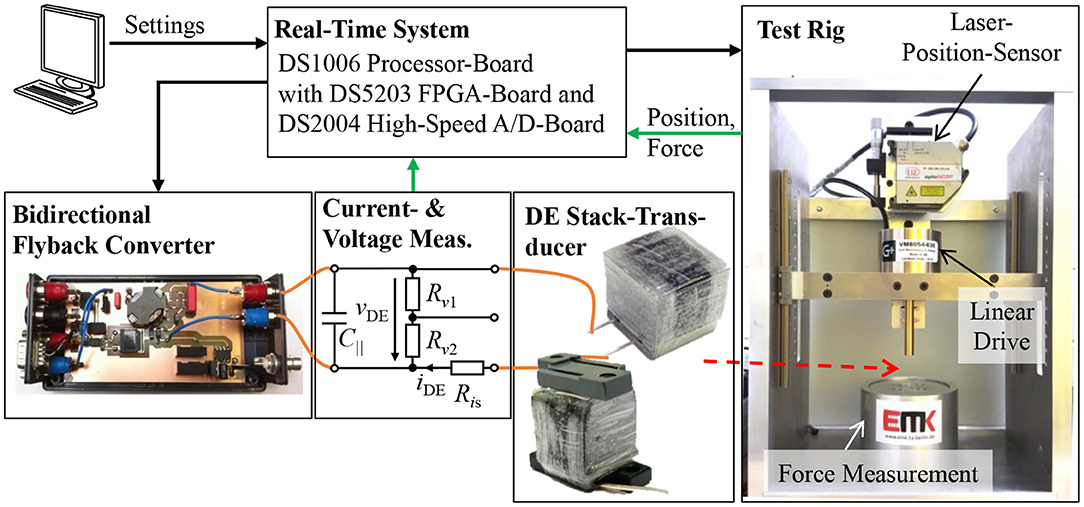
Figure 5. Test setup for the experimental validation comprising a bidirectional flyback converter, a voltage and current measurement, a DE stack-transducer and a test rig with linear drive, while the data logging and the different controls are implemented on the real-time system.

The proposed self-sensing algorithm and the energy control are implemented on the DSP of a real-time system from dSPACE operating with a sample rate of f_DSP = 20 kHz. The system contains also a fast FPGA board. On this board the control of the flyback converter and the signal conditioning for the measured voltage and current v_DE,m and i_DE,m are performed.

5.2. Validation of the EKF-Based Self-Sensing Algorithm

Before the closed-loop self-sensing operation is investigated, the estimation results obtained with the suggested self-sensing approach are compared to results estimated with the sensor-based observer introduced in Hoffstadt and Maas (2017, 2018b). The parameters of the silicone based DE stack-transducer with N = 192 layers are listed in Table 1. This table also includes parameters for the controller used in the following section.

TABLE 1

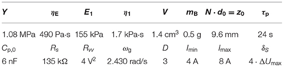
Table 1. Parameters of the utilized silicone based DE stack-transducer and the self-sensing controller.

Figure 6 compares the estimation results of the proposed self-sensing approach with the sensor-based estimator. The voltage controlled bidirectional flyback converter supplies the DE stack-transducer stepwise with voltages of v_DE = 1.5, 2.5, and 2 kV, respectively. The charge q_p determined by filtering the measured current i_DE,m according to Equation (10) is used as input for the self-sensing filter, while the sensor-based estimator uses the energy U_c,diel as input.

FIGURE 6

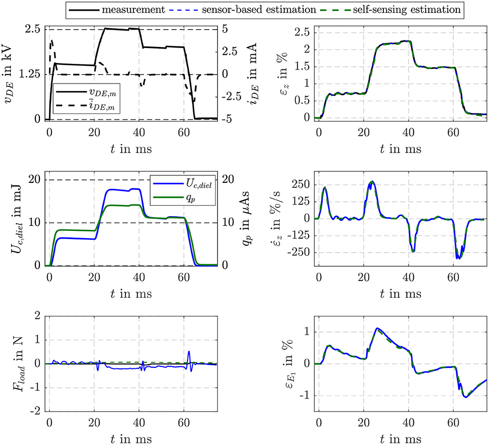
Figure 6. Comparison of the EKF-based estimation results of the proposed self-sensing filter with a sensor-based filter for the no-load scenario.

The measurement noise R_vv = 4 V² required for the implementation of the EKF can be determined experimentally. For this, the output function g_qv in Equation (13) and the properties of the voltage probe and current measurement via the shunt have to be taken into account. One of the main issues when designing an EKF is to find an appropriate choice of Q_ww. Here, the numerical optimization approach presented by Powell (2002) is used to minimize the error between simulated and estimated state variables by varying the entries of the symmetric matrix Q_ww. For the system introduced in section 3 this optimization yields:

$\begin{array}{l}{Q}_{ww,qv}\\ ={\zeta }_{qv}·\left[\begin{array}{cccc}4,8·{10}^{-8}& -1,7·{10}^{-9}& -2,2·{10}^{-8}& -9,3·{10}^{-4}\\ -1,7·{10}^{-9}& 4,9·{10}^{-5}& 1,5·{10}^{-4}& 4,4·{10}^{-1}\\ -2,2·{10}^{-8}& 1,5·{10}^{-4}& 1,6·{10}^{-9}& -1,7·{10}^{-5}\\ -9,3·{10}^{-4}& 4,4·{10}^{-1}& -1,7·{10}^{-5}& 7,6·{10}^4\end{array}\right].& (40)\end{array}$

The entries represent in a certain way the uncertainty of the model (13) to describe the dynamics of the state variables. While all entries of the matrix are comparable small, the one in the fourth row and column is very large. This is due to the unknown dynamics of the load tension that is considered with ${\dot{\sigma }}_{\text{load}}=0$ in Equation (13). As the dynamics of the state estimation can be adjusted by the absolute values of the entries in Q_ww the scaling factor ζ_qv is introduced. It gives the opportunity to adjust a compromise between sufficient dynamics, reliable state estimation and noise suppression.

In Figure 6 the no-load scenario with F_load = A · σ_load = 0 is considered. As can be seen in the comparison of the measured and estimated strains ε_z in the top right plot, almost no deviations between the approaches in terms of dynamics and accuracy occur. Due to parameter deviations the sensor-based filter estimates small load forces especially during transient operation. For the self-sensing filter with ${\zeta }_{qv}=10^{-3}$ a comparable small factor is applied here. With this negligible deviations in the estimated load force occur without affecting the estimation results of the state variables shown on the right.

Figure 7 compares the estimation results obtained when a load force of F_load = 2 N is stepwise applied to the DE stack-transducer with the force controlled voice coil actuator. When the tensile load is applied the strain of the DE transducer reduces from ε_z ≈ 1.9% to ε_z ≈ 1.1%. In voltage controlled operation this causes a reduction of charge and energy as can be seen in the top left plot. The saw tooth profile in the charge q_p and energy U_c,diel is caused by the voltage control of the flyback converter that is based on a hysteresis controller. The sensor-based filter estimates the strain as well as the load force with errors less than |err_ε| ≤ 1% and |err_F| ≤ 4%, respectively. For the self-sensing filter two parameterization with ${\zeta }_{qv}=10^{-3}$ and ζ_qv = 1 are investigated. While with ${\zeta }_{qv}=10^{-3}$ the strain and force are estimated with errors below |err_ε| ≤ 1% before the load is applied and after it is released, the dynamics of the estimation is not sufficient to consider the influence of the load correctly. In contrast, with ζ_qv = 1 the influence of the load is accurately estimated. However, with this setting the noise suppression especially for charge states below q_p ≤ 5 μAs is not sufficient. Therefore, for the following investigations of the self-sensing control the scaling factor is switched from ${\zeta }_{qv}=10^{-3}$ to ζ_qv = 1 if the charge exceed q_p ≤ 5 μAs. This ensures an accurate estimation of the inner transducer states at low charge states as well as an accurate detection of a load force and its influence on the states.

FIGURE 7

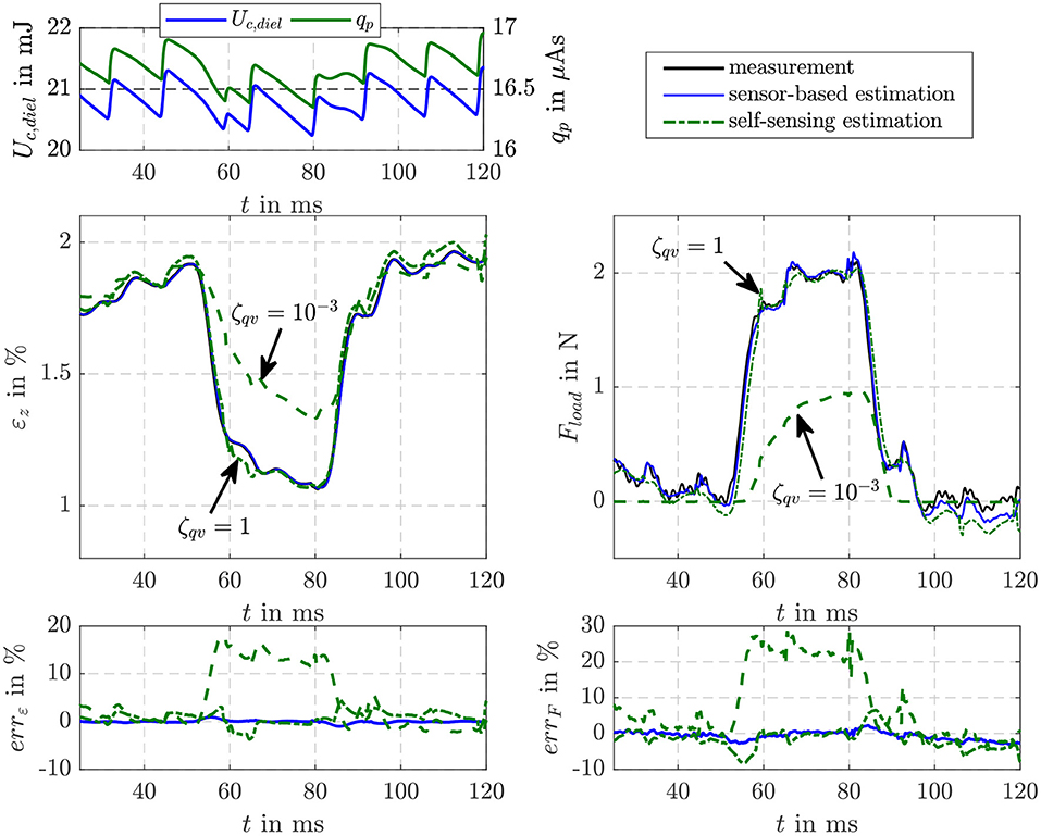
Figure 7. Comparison of the EKF-based estimation results of the proposed self-sensing filter with a sensor-based filter when a load force is applied to the DE transducer.

5.3. Validation of the Self-Sensing Control

The parameters of the sliding mode energy controller designed in section 4 are listed in Table 1. The damping coefficient D = 3 and cut-off frequency ω_g = 2.430 rad/s were determined with Equation (34). The hysteresis threshold δ_S = 4 · ΔU_max for the three-point controller in Equation (39) is set to a multiple of the energy increment ΔU_max transfered during one switching period T_S of the flyback converter. Figure 8 compares the closed-loop operation of the sensor-based controller published in Hoffstadt and Maas (2018b) and the proposed self-sensing controller. First of all, no feed-forward control approaches as suggested in Equations (20)–(22) are considered. Instead, three setpoint steps for the energy $U_{\text{c},\text{diel}}^{*}$ are applied that correspond to voltages of v_DE = 1.5 kV, 2.5 kV and 2 kV for the silicone based DE-stack-transducer, respectively. For both, the sensor-based and the self-sensing control two-point controllers (2PC) according to Equation (35) with $I_{\text{m},max}^{*}=8$ A and $I_{\text{m},max}^{*}=4$ A are investigated as well as the three-point controller (3PC) with hysteresis and adaption of the inner flyback converter control from Equation (39) and Figure 4. The DE stack-transducer is attached between the force measurement and the blocked voice coil so that it cannot deform (ε_z = 0) to avoid disturbances.

FIGURE 8

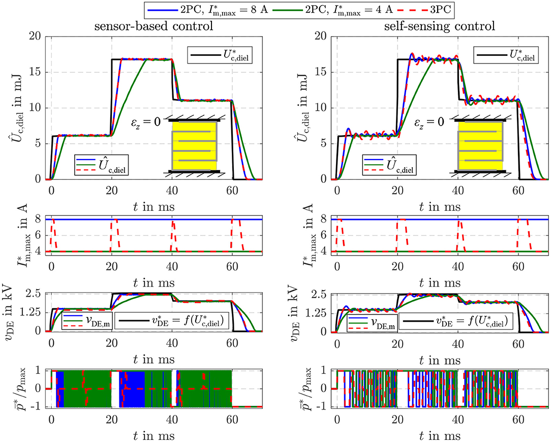
Figure 8. Comparison of the sensor-based and self-sensing sliding mode energy control. In both cases two-point controllers (2PC) with $I_{\text{m},max}^{*}=8$ A and $I_{\text{m},max}^{*}=4$ A as well as the three-point controller (3PC) with hysteresis and adaption of the inner flyback converter control are considered.

Via the setpoint $I_{\text{m},max}^{*}$ for the current control of the flyback converter its feeding power is adjusted according to Equation (5). Due to the reduced power it takes a longer time to adjust the setpoint energies with the two-point controller with $I_{\text{m},max}^{*}=4$ A compared to the one with $I_{\text{m},max}^{*}=8$ A. In contrast, the reduced feeding power results in a higher accuracy during steady state. The standard deviation for the time interval between 50 and 60 ms increases from 0.03 mJ (2PC, $I_{\text{m},max}^{*}=4$ A) to 0.05 mJ (2PC, $I_{\text{m},max}^{*}=8$ A) for the sensor-based control and from 0.1 to 0.3 mJ for the self-sensing control, respectively. The adaptive three-point controller with hysteresis combines the advantageous of the two mentioned two-point controllers by automatically choosing the maximum current $I_{\text{m},max}^{*}=8$ A right after setpoint steps and reducing this current to $I_{\text{m},max}^{*}=4$ A at steady state. This fundamental behavior applies for both the sensor-based and self-sensing control. Although the dynamics of both approaches are comparable, a small oscillation around the setpoint can be observed in case of the self-sensing control that results in the higher standard deviation.

Furthermore, it can be seen that the two-point controllers permanently switch between the maximum charging and discharging power $\bar{p}=\pm {\bar{p}}_{max}$ during steady state. By extending the controller to a three-point controller with hysteresis, the switching frequency can be significantly reduced by more than 80% in case of the sensor-based control and 30% in case of the self-sensing control.

Figure 9 depicts the comparison of the bandwidth of the introduced controller settings. For this purpose, the small signal behavior is considered. A harmonic setpoint $U_{\text{c},\text{diel}}^{*}$ with increasing frequency, an offset of Ū_c,diel = 12 mJ and an amplitude of U_c,diel,amp = 2 mJ is applied. The sensor-based two-point controller with $I_{\text{m},max}^{*}=8$ A and the three-point controller have a high -3 dB cut-off frequency of about 400 Hz. This is also obtained with the self-sensing control. However, disruptive amplitude peaks of about 5 dB result in the already observed oscillation. By reducing the feeding power $\bar{p}$ with $I_{\text{m},max}^{*}=4$ A, the cut-off frequency is reduced to 200 Hz, while the amplitude peaks are suppressed.

FIGURE 9

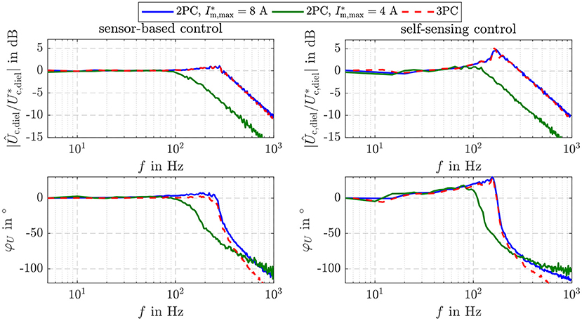
Figure 9. Bandwidth of the sensor-based and self-sensing sliding mode energy control for the three investigated controller settings.

5.4. Energy Control With Voltage Feed-Forward Control

By applying Equation (22) for the feed-forward control depicted in Figure 4 the voltage v_p across the capacitance C_p can be controlled. In Figure 10 the results of the sensor-based and self-sensing energy three-point controller are compared to the behavior obtained with the hysteresis voltage control for the bidirectional flyback converter suggested in Hoffstadt and Maas (2016).

FIGURE 10

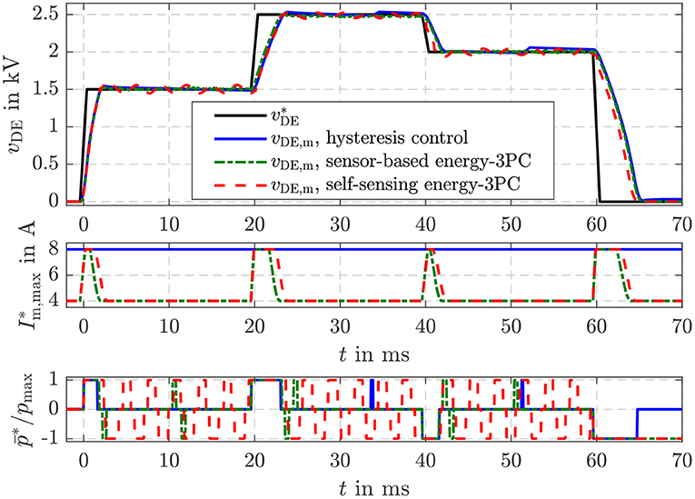
Figure 10. Comparison of a simple hysteresis voltage control with the sensor-based and self sensing energy three-point controller using a voltage feed-forward control.

For the hysteresis voltage control a threshold of Δv_DE = 30 V was chosen. If the control deviation $|v_{\text{DE}}^{*}-v_{\text{DE},\text{m}}|$ exceeds this threshold the control activates the flyback converter to charge or discharge the DE transducer. Afterwards the converter is turned into idle state again. The three-point controller suggested here behaves more or less the same. The only difference is that with the controller settings from Table 1 a threshold of v_p ≈ 16 V results. This smaller threshold increases on the one hand the steady state accuracy. However, the switching frequency is on the other hand a bit higher compared to the simple hysteresis voltage control. Concerning the sensor-based and self-sensing energy control a comparable behavior as shown and explained in Figure 8 can be observed here, too.

5.5. Energy Control With Position Feed-Forward Control

If the setpoint energy $U_{\text{c},\text{diel}}^{*}$ of the control structure in Figure 4 is determined with Equation (20) the proposed energy control can be used to adjust a certain strain ${\epsilon }_z^{*}$, although the strain is not part of the state vector x_U. To compensate the influence of a disturbance, the estimated load ${\widehat{\sigma }}_{\text{load}}$ is considered in Equation (20). In contrast, an explicit position control based on the model (6) was derived in Hoffstadt and Maas (2017). Figure 11 shows the comparison of the explicit (Position-3PC) and energy-based position control (Energy-3PC) for the no-load case of the DE stack-transducer. Both approaches are realized as sensor-based and self-sensing control with the adaptive three-point controller from Equation (39).

FIGURE 11

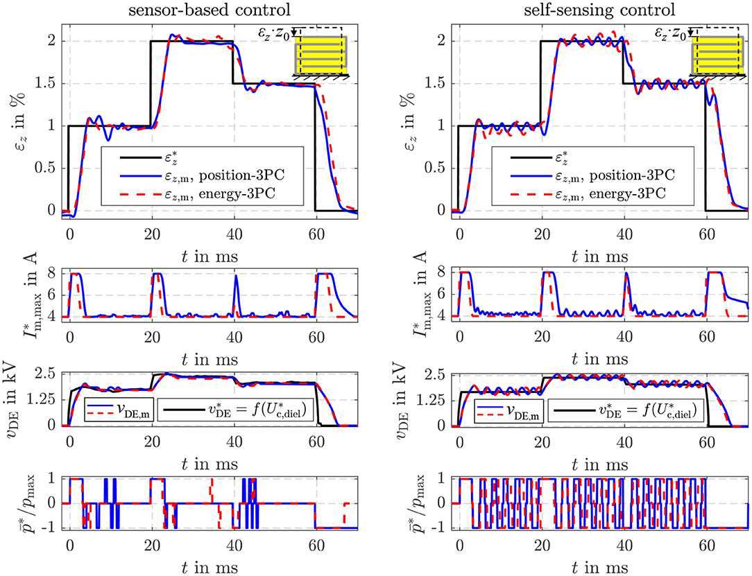
Figure 11. Comparison of the sensor-based and self-sensing energy control with position feed-forward control and an explicit sliding mode position control.

The explicit and energy-based position control show comparable dynamics and accuracy for both the sensor-based and the self-sensing control. The different setpoints are adjusted within a few milliseconds. By increasing the strain setpoint ${\epsilon }_z^{*}$ the energy $U_{\text{c},\text{diel}}^{*}$ also increases according to Equation (20). Instead of the energy, the voltage v_DE is depicted in Figure 11 as it is measured directly and can be interpreted more intuitively. With Equation (22) a relationship between the voltage v_p ≈ v_DE is given. As the no-load case is considered here, for a constant setpoint of the strain ${\epsilon }_z^{*}$ a constant setpoint for the energy $U_{\text{c},\text{diel}}^{*}$ or the voltage results, respectively.

In addition, Figure 12 depicts the disturbance reaction of the different position control approaches. For this purpose, a tensile load force of $F_{\text{load}}^{*}=$ 0.5 N is applied by the linear drive of the test rig in Figure 5, while the setpoint strain is constantly set to ${\epsilon }_z^{*}=$ 1%. Right after the load is applied, the strain deviates from its setpoint due to the influence of the disturbance. However, the load is estimated with the sensor-based as well as the self-sensing EKF. According to Equation (20) the setpoint energy $U_{\text{c},\text{diel}}^{*}$, or voltage $v_{\text{DE}}^{*}$, respectively, is increased to compensate the influence of the disturbance ${\widehat{\sigma }}_{\text{load}}$. In Figure 12 this behavior can be seen in the response of the corresponding voltage v_DE in the third subplot. This compensates the influence of the disturbance within approx. 15 ms. In case of the energy-based position control a slightly higher control deviation can be observed after the load steps. This is mainly due to the fact, that the energy control only reacts on control deviations of the energy U_c,diel, while the explicit position control considers the control deviation of the strain ε_z directly.

FIGURE 12

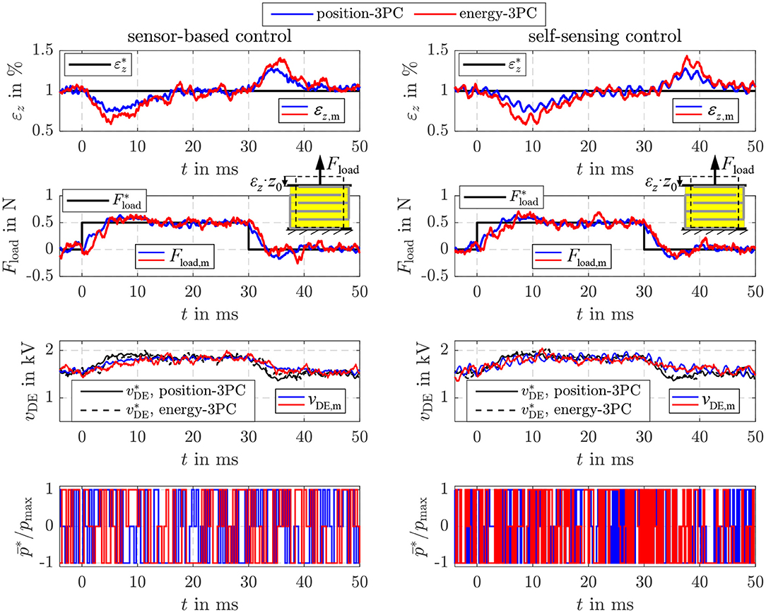
Figure 12. Disturbance reaction of the sensor-based and self-sensing energy control with position feed-forward control and an explicit sliding mode position control.

5.6. Energy Control With Force Feed-Forward Control

Beside the two validated approaches, Equation (21) offers the opportunity to realize a force feed-forward control under consideration of the current elastic material tension ${\sigma }_{\text{elast}}({\widehat{\epsilon }}_z)$ based on the proposed energy control as already depicted in Figure 4. As for the previous two approaches, the controller settings are the same as listed in Table 1. However, in Figure 13 also the two-point controller with I_m,max = 8 A and I_m,max = 4 A is considered again. The deformation of the DE stack-transducer is blocked in this case to investigate the control behavior caused by setpoint steps without any disturbance. In general, a comparable behavior to the pure energy control in Figure 8 can be observed here, too. According to Equation (21) a constant energy setpoint $U_{\text{c},\text{diel}}^{*}$ is obtained for a certain force $F_{\text{act}}^{*}$ and ε_z = 0. In comparison to the two-point controllers the adaptive three-point controller from Equation (39) ensures the highest possible dynamics by the maximum current I_m,max = 8 A during transient operation as well as good steady state accuracy with significantly reduced switching frequency by reducing the current to I_m,max = 4 A. The self-sensing control adjusts the different setpoint forces with dynamics that are absolutely comparable to the sensor-based control.

FIGURE 13

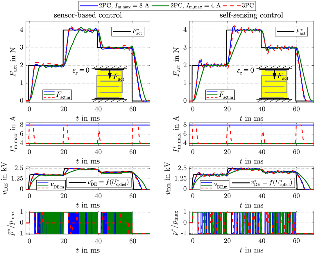
Figure 13. Comparison of the sensor-based and self-sensing sliding mode energy control with force feed-forward control. In both cases two-point controllers (2PC) with $I_{\text{m},max}^{*}=8$ A and $I_{\text{m},max}^{*}=4$ A as well as the three-point controller (3PC) with hysteresis and adaption of the inner flyback converter control are considered.

In Figure 14 also the disturbance reaction of the energy-based force control is shown. In this case a variable strain ε_z adjusted by the position-controlled linear drive acts as a disturbance. The stepwise change of the strain to ${\epsilon }_z^{*}=$ 1% causes a reduction of the force F_act in the first moment. However, by increasing the setpoint energy $U_{\text{c},\text{diel}}^{*}$, or voltage $v_{\text{DE}}^{*}$, respectively, according to Equation (21) the influence is compensated comparable to the behavior observed for the disturbance reaction of the energy-based position control in Figure 12. The sensor-based control offers a marginal better control quality what is caused by the slightly higher dynamics of the sensor-based state and disturbance estimation.

FIGURE 14

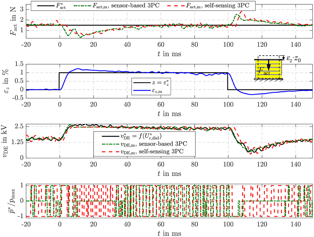
Figure 14. Disturbance reaction of the sensor-based and self-sensing energy control with force feed-forward control.

The investigation of the pure energy control in Figures 8, 9 as well as of the different feed-forward controls in the Figures 10–14 proved that both high dynamics and good steady state accuracy are obtained with the proposed self-sensing control approach. The developed self-sensing EKF estimates not only the inner states of the DE transducer but also an external load tension. In case of the position feed-forward control this allows to compensate the influence of a disturbance load. In contrast, if the force feed-forward control is applied the elastic material tension caused by a deformation of the DE transducer is reliably compensated. Furthermore, extensions to an adaptive three-point controller enabled a reduction of the switching frequency of up to 80% to increase the energy efficiency without reducing the bandwidth of about 400 Hz and the steady state accuracy.

6. Conclusion

DE transducer combine high energy densities and multi-functional operation modes. Multilayer topologies like the DE stack-actuator considered here have also high force densities with considerable absolute deformations so that they are well-suited to be used as active skins or as end effector in soft-robotic applications. But, beside the transducer design also appropriate control and sensing algorithms are required to enable the combined actuator-sensor-operation in closed loop operation without external sensors to measure mechanical states. The design of such a self-sensing state and disturbance estimator as a universal energy control that uses the information from a novel self-sensing estimator were addressed within this contribution.

For this purpose, in section 2 the control plant comprising a DE stack-transducer fed by a bidirectional flyback converter and its model to describe the electormechanically coupled behavior was summarized. To characterize the electrical behavior the model includes the energy U_c,diel as one state variable. Based on this model subsequently a self-sensing state and disturbance estimator was developed that estimates the mechanical state of the transducer as well as an external load force by just measuring the terminal voltage and current. Due to the non-linear system behavior an EKF was used for this purpose. It allows to estimate the transducer state without any superimposed voltage excitation as used for other self-sensing approaches. The validation results have shown that almost no confinements in terms of dynamics and accuracy compared to the sensor-based estimator are obtained. The sensor-based estimator requires a measurement of the terminal voltage and the displacement.

The developed energy control uses the information provided by the self-sensing EKF for closed loop operation. Due to the behavior of the bidirectional flyback converter, that either charges or discharges a DE transducer with almost constant power when enabled, the sliding mode control approach was applied. By controlling the energy in the capacitance of the DE transducer it is possible to control the voltage, force or displacement of the transducer by using different feed-forward control structures. The setpoint energy required to achieve a certain actuator force or displacement was obtained under consideration of the static force equilibrium included in the derived model. Within the validation it was shown that a precise control of the voltage, force and displacement with high dynamics and a bandwidth of up to 400 Hz is achieved with this approach. The step response as well as the disturbance reaction yield comparable dynamics and accuracy for both the sensor-based and self-sensing control.

Although here a DE stack-transducer was considered, the developed self-sensing EKF and control approach can also be applied to other topologies well-suited for soft robotic applications like DE-based minimum energy structures or membrane actuators. The utilized bidirectional flyback converter represents an efficient and competitive converter topology and can also be used to supply any kind of DE transducer. In case of soft-bodied robots equipped with DE transducers and the mentioned converter the suggested self-sensing control approach can be used to control the impedance of the robot by applying the proposed force and displacement feed-forward controls in combination with a human-machine-interface model. If under consideration of the utilized test setup a charge of at least q_p = 5 μAs is applied, the proposed self-sensing filter can also detect collisions or interactions. This could be used e.g., in human machine interfaces or active skins, so that the control can react on these events. While for these applications the force and displacement control are most important, the voltage control could be used to avoid exceeding limitations that would cause a damage of the transducer.

Data Availability Statement

The raw data supporting the conclusions of this manuscript will be made available upon request to JM ( juergen.maas@tu-berlin.de).

Author Contributions

The research results included in this contribution are the outcome of TH's Ph.d. thesis that was supervised by JM.

Conflict of Interest

The authors declare that the research was conducted in the absence of any commercial or financial relationships that could be construed as a potential conflict of interest.

References

Adamy, J. (2014). Nichtlineare Systeme und Regelungen, 2nd Edn. Berlin: Springer Vieweg.

Google Scholar

Anderson, I. A., Gisby, T. A., McKay, T. G., O'Brien, B. M., and Calius, E. P. (2012). Multi-functional dielectric elastomer artificial muscles for soft and smart machines. J. Appl. Phys. 112:041101. doi: 10.1063/1.4740023

CrossRef Full Text | Google Scholar

Chuc, N. H., Thuy, D. V., Park, J., Kim, D., Koo, J., Lee, Y., et al. (2008). A dielectric elastomer actuator with self-sensing capability. Proc. SPIE 6927:69270V. doi: 10.1117/12.777900

CrossRef Full Text | Google Scholar

DeCarlo, R. A., Zak, S. H., and Matthews, G. P. (1988). Variable structure control of nonlinear multivariable systems: a tutorial. Proc. IEEE 76, 212–232. doi: 10.1109/5.4400

CrossRef Full Text | Google Scholar

Dubois, P., Rosset, S., Niklaus, M., Dadras, M., and Shea, H. (2008). Voltage control of the resonance frequency of dielectric electroactive polymer (deap) membranes. J. Microelectromech. Syst. 17, 1072–1081. doi: 10.1109/JMEMS.2008.927741

CrossRef Full Text | Google Scholar

Eitzen, L., Graf, C., and Maas, J. (2011a). “Bidirectional high voltage dc-dc converters for energy harvesting with dielectric elastomer generators,” in IEEE Energy Conversion Congress & Exposition (ECCE'11) (Arizona).

Google Scholar

Eitzen, L., Graf, C., and Maas, J. (2011b). “Cascaded bidirectional flyback converter driving deap transducers,” in 37th Annual Conference of the IEEE Industrial Electronics Society IECON-2011, (Melbourne), 1226–1231. doi: 10.1109/IECON.2011.6119484

CrossRef Full Text | Google Scholar

Gisby, T. A., O'Brien, B. M., and Anderson, I. A. (2013). Self sensing feedback for dielectric elastomer actuators. Appl. Phys. Lett. 102:193703. doi: 10.1063/1.4805352

CrossRef Full Text | Google Scholar

Gisby, T. A., O'Brien, B. M., Xie, S. Q., Calius, E. P., and Anderson, I. A. (2011). Closed loop control of dielectric elastomer actuators (SPIE). SPIE Proc. 7976. doi: 10.1117/12.880711

CrossRef Full Text | Google Scholar

Hoffstadt, T., Griese, M., and Maas, J. (2014). Online identification algorithms for integrated dielectric electroactive polymer sensors and self-sensing concepts. Smart Mater. Struct. 23:1–13. doi: 10.1088/0964-1726/23/10/104007

CrossRef Full Text | Google Scholar

Hoffstadt, T., and Maas, J. (2015). Analytical modeling and optimization of deap-based multilayer stack-transducers. Smart Mater. Struct. 24:1–14. doi: 10.1088/0964-1726/24/9/094001

CrossRef Full Text | Google Scholar

Hoffstadt, T., and Maas, J. (2016). Sensorless bcm control for a bidirectional flyback-converter. IEEE IECON 2016 42, 3600–3605. doi: 10.1109/IECON.2016.7793842

CrossRef Full Text | Google Scholar

Hoffstadt, T., and Maas, J. (2017). Adaptive sliding-mode position control for dielectric elastomer actuators. IEEE/ASME Trans. Mechatr. 22, 2241–2251. doi: 10.1109/TMECH.2017.2730589

CrossRef Full Text | Google Scholar

Hoffstadt, T., and Maas, J. (2018a). Model-based self-sensing algorithm for dielectric elastomer transducers based on an extended Kalman filter. Mechatronics 50, 248–258. doi: 10.1016/j.mechatronics.2017.09.013

CrossRef Full Text | Google Scholar

Hoffstadt, T., and Maas, J. (2018b). Sensorless force control for dielectric elastomer transducers. J. Intell. Mater. Syst. Struct. 30. doi: 10.1177/1045389X17754255

CrossRef Full Text | Google Scholar

Hoffstadt, T., Meier, P., and Maas, J. (2016). “Modeling approach for the electrodynamics of multilayer de stack-transducers,” in ASME 2016 Conference on Smart Materials, Adaptive Structures and Intelligent Systems V001T02A015 (Florence).

Google Scholar

Ifeachor, E. C., and Jervis, B. W. (2002). Digital Signal Processing: A Practical Approach, 2nd Edn. Harlow: Prentice Hall.

Isermann, R., and Munchhof, M. (2011). Identification of Dynamical Systems: An Introduction With Applications. Advanced textbooks in control and signal processing. Berlin; London: Springer.

Google Scholar

Jung, K., Kim, K. J., and Choi, H. R. (2008). A self-sensing dielectric elastomer actuator. Sens. Actuat. A 143, 343–351. doi: 10.1016/j.sna.2007.10.076

CrossRef Full Text | Google Scholar

Kaal, W., and Herold, S. (2011). Electroactive polymer actuators in dynamic applications. IEEE/ASME Trans. Mechatr. 16, 24–32. doi: 10.1109/TMECH.2010.2089529

CrossRef Full Text | Google Scholar

Kalman, R. E. (1960). Contributions to the theory of optimal control. Boletin de la Sociedad 5, 102–119

Google Scholar

Kuhring, S., Uhlenbusch, D., Hoffstadt, T., and Maas, J. (2015). Finite element analysis of multilayer deap stack-actuators. Proc. SPIE 9430:94301L. doi: 10.1117/12.2085121

CrossRef Full Text | Google Scholar

Maas, J., Graf, C., and Eitzen, L. (2011). Control concepts for dielectric elastomer actuators. Proc. SPIE 7976:79761H. doi: 10.1117/12.879938

CrossRef Full Text | Google Scholar

Maas, J., Tepel, D., and Hoffstadt, T. (2015). Actuator design and automated manufacturing process for deap-based multilayer stack-actuators. Meccanica 50, 2839–2854. doi: 10.1007/s11012-015-0273-2

CrossRef Full Text | Google Scholar

Matysek, M., Haus, H., Moessinger, H., Brokken, D., Lotz, P., and Schlaak, H. F. (2011). Combined driving and sensing circuitry for dielectric elastomer actuators in mobile applications (SPIE). SPIE Proc. 7976:1–11. doi: 10.1117/12.879438

CrossRef Full Text

Navarro, S. E., Marufo, M., Ding, Y., Puls, S., Goger, D., Hein, B., et al. (2013). “Methods for safe human-robot-interaction using capacitive tactile proximity sensors,” in 2013 IEEE/RSJ International Conference, 1149–1154. doi: 10.1109/IROS.2013.6696495

CrossRef Full Text | Google Scholar

Powell, T. D. (2002). Automated tuning of an extended kalman filter using the downhill simplex algorithm. J. Guid. Cont. Dyn. 25, 901–908. doi: 10.2514/2.4983

CrossRef Full Text | Google Scholar

Rizzello, G., Naso, D., York, A., and Seelecke, S. (2015). Modeling, identification, and control of a dielectric electro-active polymer positioning system. IEEE Trans. Control Syst. Technol. 23, 632–643. doi: 10.1109/TCST.2014.2338356

CrossRef Full Text | Google Scholar

Rizzello, G., Naso, D., York, A., and Seelecke, S. (2016). Closed loop control of dielectric elastomer actuators based on self-sensing displacement feedback. Smart Mater. Struct. 25:035034. doi: 10.1088/0964-1726/25/3/035034

CrossRef Full Text | Google Scholar

Rizzello, G., Naso, D., York, A., and Seelecke, S. (2017). A self-sensing approach for dielectric elastomer actuators based on online estimation algorithms. IEEE/ASME Trans. Mechatr. 22, 728–738. doi: 10.1109/TMECH.2016.2638638

CrossRef Full Text | Google Scholar

Robla-Gomez, S., Becerra, V. M., Llata, J. R., Gonzalez-Sarabia, E., Torre-Ferrero, C., and Perez-Oria, J. (2017). Working together: a review on safe human-robot collaboration in industrial environments. IEEE Access 5, 26754–26773. doi: 10.1109/ACCESS.2017.2773127

CrossRef Full Text | Google Scholar

Rosset, S., O'Brien, B. M., Gisby, T., Xu, D., Shea, H. R., and Anderson, I. A. (2013). Self-sensing dielectric elastomer actuators in closed-loop operation. Smart Mater. Struct. 22:104018. doi: 10.1088/0964-1726/22/10/104018

CrossRef Full Text | Google Scholar

Sarban, R. (2011). Active vibration control using DEAP transducers. (Dissertation). University of Southern Denmark, Sønderborg, Denmark.

Google Scholar

Sarban, R., and Jones, R. W. (2012). Physical model-based active vibration control using a dielectric elastomer actuator. J. Intell. Mater. Syst. Struct. 23, 473–483. doi: 10.1177/1045389X11435430

CrossRef Full Text | Google Scholar

Welch, G., and Bishop, G. (2001). An Introduction to the Kalman Filter. Chapel Hill: University of North Carolina.

Google Scholar

Wilson, E. D., Assaf, T., Pearson, M. J., Rossiter, J. M., Anderson, S. R., Porrill, J., et al. (2016). Cerebellar-inspired algorithm for adaptive control of nonlinear dielectric elastomer-based artificial muscle. J. R. Soc. Interface 13:1–15. doi: 10.1098/rsif.2016.0547

PubMed Abstract | CrossRef Full Text | Google Scholar