Simulation Evaluation for Methods Used to Determine Muscular Internal Force Based on Joint Stiffness Using Muscular Internal Force Feedforward Controller for Musculoskeletal System

1 Introduction

Humans are able to easily achieve specific complex movements by manipulating the structure of the human body. The human body structure can be described in terms of a musculoskeletal structure in which muscles, corresponding to actuators, cover bones and joints. Joint angle and stiffness can be adjusted by contracting the muscles, thus allowing the individual to perform complex motions.

A number of robots that can imitate this musculoskeletal structure have recently been investigated. Marques et al. (Marques et al., 2010) developed a human coexistence robot that imitates the musculoskeletal structure, while a research group including Inaba (Mizuuchi et al., 2006; Asano et al., 2016) developed another musculoskeletal structure-imitating humanoid robot. Verrelst et al. (Verrelst et al., 2005) developed a biped robot actuated with antagonistic pneumatic artificial muscles. This robot can control joint stiffness and achieve stable walking. Niiyama et al. (Niiyama et al., 2012) developed a double legged robot with a musculoskeletal structure that emulates an athlete’s physique and style of running. Their robot had the capability of running stably for 4 m. Niiyama et al. (Niiyama et al., 2007) developed a jumping robot with a musculoskeletal structure that could perform big leaps. The results of these studies indicate that the musculoskeletal structure functions as a feedback system when undergoing instantaneous movements; thus, an understanding of the musculoskeletal structure can be used to develop robots that can perform previously difficult-to-achieve motions.

In a previous study, we proposed a muscular internal force (MIF) feedforward controller for a musculoskeletal system (Kino et al., 2009, 2013). This controller could be used to attain any desired position without the use of sensors, by providing a MIF as a feedforward input to the associated muscle. The controller input would create a potential field in the musculoskeletal system; allowing the system to converge at the desired position when this potential field achieved a stable equilibrium point at the desired position. This end-point convergence is influenced by muscle arrangement (Kino et al., 2017). The MIF must be increased to obtain a desirable control response, through increase in system stiffness. Subsequently, reducing the MIF to lower the stiffness causes the responsiveness to deteriorate. As a result of the correlation between response and stiffness, it is challenging to simultaneously achieve high-response motion and low system stiffness. Furthermore, the controller is affected by an ill-posed problem where, its input cannot be uniquely determined due to the muscle redundancy of the musculoskeletal system.

To tackle this muscle redundancy, Buchler et al. (Buchler et al., 2018) proposed a variance-regularized control that can achieve high accuracy trajectory tracking in the musculoskeletal system. In addition, Jantsch et al. (Jantsch et al., 2011) proposed a new controller based on computed torque control and a method for obtaining the muscle Jacobian by using machine-learning techniques for the musculoskeletal system. Their method indicates that trajectory control and force control can be achieved. Katayama and Kawato (Katayama and Kawato, 1990) proposed a parallel-hierarchical neural network model based on a feedback-error-learning scheme, in the field of exercise physiology. This model requires repeated trials; however, it is capable of achieving rapid movements that have otherwise been difficult to achieve using a feedback controller. A tendon driven robot equivalent to the musculoskeletal system has been explored (Viau et al., 2015). However, position control methods, like the feedforward controller method from our previous study (Kino et al., 2009, 2013), have not been fully explored.

Further, various studies have been conducted on methods for contributive employment of redundancies (Klein and Huang, 1983). For instance, it has been observed that redundancy can be used to avoid specific robot attitudes (Mayorga and Wong, 1988) and obstacles (Baillieul, 1986; Chirikjian and Burdick, 1990) during motion. In addition, redundancies can be used to optimize torques in the robotic structure (Suh and Hollerbach, 1987), avoid restrictive joint movement (Shimizu et al., 2008), and apply stiffness (Svinin et al., 2002) and impedance control (Albu-Schaffer et al., 2003). Yoshikawa (Yoshikawa, 1985) suggested that the operability of a manipulator can be improved using redundancy; while, Hanafusa et al. (Hanafusa et al., 1981) and Nakamura et al. (Nakamura and Hanafusa, 1987) proposed control methods for achieving sub-tasks, based on the prioritization of robot actions. In parallel wire-driven systems (Sui and Zhao, 2004; Behzadipour and Khajepour, 2006), system actuation redundancy can be used to generate internal wire forces. The stiffness of the system can be changed by controlling these internal forces, thus indicating that robot performance and versatility can be improved by manipulating the robot’s redundancy. Hence, redundancy has several potential advantages. Meanwhile, sensors are mostly utilized in methods that employ redundancy. The musculoskeletal system continues to encounter muscle redundancy. The musculoskeletal system can achieve various kinds of motion by utilizing muscle redundancy without the addition of a new actuator.

The primary objective of this study is, to resolve the issues in the MIF feedforward controller proposed in previous studies. We began by eliminating the foremost issue of correlation between the response and stiffness. Further, the MIF that separately sets the response and stiffness was determined, and the ill-posed problem was solved. In this study, a new generic method for determining MIF using joint stiffness was developed, as an approach to improving the control performance of our previously developed MIF feedforward controller. The proposed method involves the application of an approach derived from Nakamura (Nakamura and Hanafusa, 1987), which includes prioritized application of sub-tasks to increase the stiffness of joints at desired positions by way of redundancy. This approach was used to develop two specific MIF determination methods: one involving the independent setting of response and stiffness, and the other involving the unique determination of MIF. The first method was used to identify the MIF that can independently determine the response and stiffness at a desired position, while the second was used to determine an arbitrary vector that reflects the stiffness at the initial and desired positions, and uniquely defines the balance of MIFs at each position.

The remainder of this paper is organized as follows. Section 2 describes the kinematics of the musculoskeletal system. Section 3 describes the MIF feedforward system used to control the musculoskeletal system. In Section 4, describes the development of a joint stiffness matrix of the musculoskeletal system. The two methods and their simulation results are presented in Sections 5 and Section 6, respectively.

2 Musculoskeletal System

The musculoskeletal system considered in this study is shown in Figure 1. The system comprised of two links and six muscles. The joint had one degree of freedom and could rotate when muscle tension was applied through the link. A joint with one degree of freedom requires at least two muscles to drive its link in the clockwise and counter-clockwise directions because muscles can only produce shrinkage forces; as a result of which, this system has an actuation redundancy. Additionally, we assumed that the movement of the system was unaffected by the force of gravity because the system was set in the x-y plane.

FIGURE 1

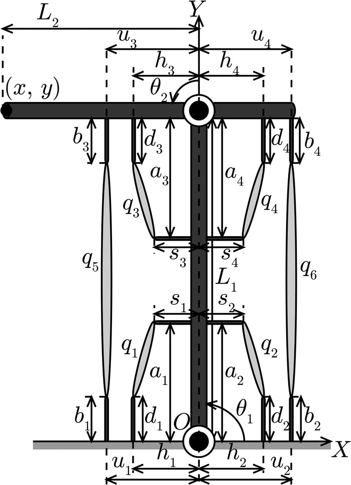
FIGURE 1. Musculoskeletal system.

The muscle consisted of a combination of wire and motor instead of a pneumatic actuator (Kino et al., 2017). The muscles were connected to an anchored base, and to each link. The anchoring was set at an explicit offset that influenced the convergence of the MIF feedforward controller (Kino et al., 2009, 2013). In our analysis of the muscular arrangement, we employed a set of parameters that converged at a desired position. Although, as mentioned above, the influence of gravity is also not considered; however, the muscular internal force feedforward controller is able to achieve system movement under the influence of gravity from a result of an other study (Matsutani et al., 2019b).

2.1 Relation Between Muscle and Joint Spaces

The relation between the muscle length vector $\mathit{q}\left(\mathit{\theta }\right)={[q_1,\dots ,q_6]}^{\mathrm{T}}$ and the joint angle vector $\mathit{\theta }={[{\theta }_1,{\theta }_2]}^{\mathrm{T}}$ within the musculoskeletal system is given by

$\mathit{q}(\mathit{\theta })=\left[\begin{array}{c}\sqrt{{(h_1+a_1{C}_1-s_1{S}_1)}^2+{(d_1-a_1{S}_1-s_1{C}_1)}^2}\hfill \\ \sqrt{{(h_2-a_2{C}_1-s_2{S}_1)}^2+{(d_2-a_2{S}_1+s_2{C}_1)}^2}\hfill \\ \sqrt{{(h_3+a_3{C}_2-s_3{S}_2)}^2+{(d_3-a_3{S}_2-s_3{C}_2)}^2}\hfill \\ \sqrt{{(h_4-a_4{C}_2-s_4{S}_2)}^2+{(d_4-a_4{S}_2+s_4{C}_2)}^2}\hfill \\ \sqrt{{(u_1+L_1{C}_1+u_3{C}_{12}-b_3{S}_{12})}^2+{(b_1-L_1{S}_1-u_3{S}_{12}-b_3{C}_{12})}^2}\hfill \\ \sqrt{{(u_2-L_1{C}_1+u_4{C}_{12}+b_4{S}_{12})}^2+{(b_2-L_1{S}_1+u_4{S}_{12}-b_4{C}_{12})}^2}\hfill \end{array}\right],(1)$

where L_i (i = 1, 2) is the link length, a_j (j = 1, … , 4), b_j, d_j, h_j, u_j, s_j are the muscular arrangement parameters, as shown in Figure 1, C_i and S_i are defined in terms of i as C_i = cos θ_i and S_i = sin θ_i, respectively, and C₁₂ and S₁₂ are defined as C₁₂ = cos (θ₁ + θ₂) and S₁₂ = sin (θ₁ + θ₂), respectively. By differentiating Eq. 1 with respect to time, the relation between the muscle contractile vector $\dot{\mathit{q}}(\mathit{\theta })\in {\mathbb{R}}^6$ and the joint angular velocity vector $\dot{\mathit{\theta }}\in {\mathbb{R}}^2$ can be obtained:

$\dot{\mathit{q}}(\mathit{\theta })=-\mathit{W}{(\mathit{\theta })}^{\mathrm{T}}\dot{\mathit{\theta }},(2)$

where $\mathit{W}(\mathit{\theta })\in {\mathbb{R}}^{2\times 6}$ is the Jacobi matrix showing the relation between the respective vectors, which is given by

$\mathit{W}(\mathit{\theta })=-\frac{\partial \mathit{q}{(\mathit{\theta })}^{\mathrm{T}}}{\partial \mathit{\theta }}.(3)$

The relation between the joint torque vector $\mathit{\tau }(\mathit{\theta })={[{\tau }_1(\mathit{\theta }),{\tau }_2(\mathit{\theta })]}^{\mathrm{T}}$ and the muscle tension vector $\mathit{\alpha }(\mathit{\theta })\in {\mathbb{R}}^6$ can be obtained based on the principle of virtual work as

$\mathit{\tau }(\mathit{\theta })=\mathit{W}(\mathit{\theta })\mathit{\alpha }(\mathit{\theta }).(4)$

The inverse relationship to that given in Eq. 4 is expressed as

$\begin{array}{c}\hfill \mathit{\alpha }(\mathit{\theta })=\mathit{W}{(\mathit{\theta })}^{+}\mathit{\tau }(\mathit{\theta })+\left({\mathit{I}}_6-\mathit{W}{(\mathit{\theta })}^{+}\mathit{W}(\mathit{\theta })\right){\mathit{k}}_{\mathit{e}},\end{array}(5)$

$\begin{array}{c}=\mathit{W}{(\mathit{\theta })}^{+}\mathit{\tau }(\mathit{\theta })+\mathit{v}(\mathit{\theta }),\hfill \end{array}(6)$

where ${\mathit{I}}_6\in {\mathbb{R}}^{6\times 6}$ is a unit matrix, ${\mathit{k}}_{\mathit{e}}\in {\mathbb{R}}^6$ is an arbitrary vector, $\mathit{v}(\mathit{\theta })\in {\mathbb{R}}^6$ is the MIF vector, and $\mathit{W}{(\mathit{\theta })}^{+}\in {\mathbb{R}}^{6\times 2}$ is a pseudo inverse matrix of W(θ) defined by

$\mathit{W}{(\mathit{\theta })}^{+}=\mathit{W}{(\mathit{\theta })}^{\mathrm{T}}{\left(\mathit{W}(\mathit{\theta })\mathit{W}{(\mathit{\theta })}^{\mathrm{T}}\right)}^{-1}.(7)$

The MIF vector v(θ) corresponds to the internal force applied within the muscle. This vector belongs to the null space, that is, it is a muscle tension component that cannot generate joint torque and satisfies the following equation

$\mathit{W}(\mathit{\theta })\mathit{v}(\mathit{\theta })=\mathbf{0}.(8)$

As a result, the musculoskeletal system was subjected to an ill-posed problem because the MIF vector corresponding to a given joint torque could not be uniquely determined.

2.2 Relation Between Task and Joint Spaces

The relation between the end-point position vector x(θ) = [x,y]^T and the joint angle vector θ of the musculoskeletal system is given by

$\mathit{x}(\mathit{\theta })=\left[\begin{array}{c}\hfill L_1{C}_1+L_2{C}_{12}\hfill \\ \hfill L_1{S}_1+L_2{S}_{12}\hfill \end{array}\right].(9)$

By differentiating Eq. 9 with respect to time, the relation between the end-point velocity vector $\dot{\mathit{x}}(\mathit{\theta })\in {\mathbb{R}}^2$ and the joint angular velocity vector $\dot{\mathit{\theta }}$ can be obtained as

$\dot{\mathit{x}}(\mathit{\theta })=\mathit{J}(\mathit{\theta })\dot{\mathit{\theta }},(10)$

Where $\mathit{J}(\mathit{\theta })\in {\mathbb{R}}^{2\times 2}$ is the Jacobi matrix showing the relation between the respective vectors.

3 Muscular Internal Force Feedforward Controller

The MIF feedforward controller, developed in our previous study (Kino et al., 2009, 2013) was used to positionally control the musculoskeletal system. In this method, the controller inputs a balancing MIF at a desired joint angle of θ_d into the muscles of the musculoskeletal system. This control input has been expressed using Eqs 5, 6 as

$\begin{array}{ccc}\hfill \mathit{\alpha }(\mathit{\theta })& =\hfill & \mathit{v}({\mathit{\theta }}_d)\hfill \\ \hfill & =\hfill & \left({\mathit{I}}_6-\mathit{W}{({\mathit{\theta }}_d)}^{+}\mathit{W}({\mathit{\theta }}_d)\right){\mathit{k}}_{\mathit{e}}.\hfill \end{array}(11)$

Under this method, control was obtained using only kinematics; the input of any physical parameters or sensor information of the musculoskeletal system was not required. The Jacobi matrix W (θ_d) had a constant value at all times, across all joint angular displacements because the matrix was obtained using the desired joint angle θ_d. Additionally, the control input was constant when the arbitrary vector k_e was constant.

When the shrinkage direction of the muscle was set at a positive, the muscle tension α(θ) also had a positive value because the muscle can produce only tension or shrinkage. Therefore, the elements v_dl (l = 1, … , 6) of the MIF $\mathit{v}({\mathit{\theta }}_d)={[v_{d1},\dots ,v_{d6}]}^{\mathrm{T}}$ needed to satisfy the following equation:

$v_{dl}>0.(12)$

Under this control method, the arbitrary vector k_e was set freely within a range satisfying Eq. 12.

Joint torque cannot be generated at a joint angle of θ = θ_d to the muscle, by applying the control input detailed in Eq. 11:

$\mathit{W}({\mathit{\theta }}_d)\mathit{v}({\mathit{\theta }}_d)=\mathit{0}.(13)$

The control input is a muscle tension component that does not generate joint torque because the MIF vector v (θ_d) belongs to the null space of the Jacobi matrix W (θ_d). By contrast, at joint angles of θ ≠ θ_d the control input v (θ_d) cannot be considered to be a vector belonging to the null space of W(θ). It is possible for a control input v (θ_d) to generate a joint torque because v (θ_d) can be decomposed into two components: a muscle tension component that does not generate joint torque and the vector v(θ) that belongs to the null space:

$\mathit{W}(\mathit{\theta })\mathit{v}({\mathit{\theta }}_d)=\mathbf{0}\mathrm{o}\mathrm{r}\mathit{W}(\mathit{\theta })\mathit{v}({\mathit{\theta }}_d)\ne \mathbf{0}.(14)$

Using the abovementioned characteristics, the MIF controller generated joint movement.

The convergence of the motion end-point was related to the potential P generated by the MIF v (θ_d) (Kino et al., 2009, 2013), which is defined as

$P={\left(\mathit{q}(\mathit{\theta })-\mathit{q}({\mathit{\theta }}_d)\right)}^{\mathrm{T}}\mathit{v}({\mathit{\theta }}_d).(15)$

A musculoskeletal system movement converged on a desired joint angle θ_d when the angle dependent on muscular arrangement, corresponded to a stable equilibrium point in P (Kino et al., 2009, 2013). Moreover, the muscular arrangements that were used to attain convergence were identified based on the results of our previous studies (Kino et al., 2009, 2013).

4 Joint Stiffness Matrix

The joint stiffness matrix ${\mathit{K}}_j(\mathit{\theta })\in {\mathbb{R}}^{2\times 2}$ of the musculoskeletal system (Nakiri and Kino, 2009) is given by

${\mathit{K}}_j(\mathit{\theta })=-\frac{\partial \mathit{\tau }(\mathit{\theta })}{\partial \mathit{\theta }}.(16)$

Here, because the joint torque τ(θ) was generated by the MIF controller, the joint stiffness matrix was derived from Eqs 4, 11 as follows:

$\begin{array}{ccc}\hfill \mathit{\tau }(\mathit{\theta })& =\hfill & \mathit{W}(\mathit{\theta })\left({\mathit{I}}_6-\mathit{W}{({\mathit{\theta }}_d)}^{+}\mathit{W}({\mathit{\theta }}_d)\right){\mathit{k}}_{\mathit{e}}\hfill \\ \hfill & =\hfill & \mathit{W}(\mathit{\theta })\mathit{Y}({\mathit{\theta }}_d){\mathit{k}}_{\mathit{e}}.\hfill \end{array}(17)$

For convenience, the Jacobi matrix W(θ) from Eq. 3 is rewritten as

$\mathit{W}(\mathit{\theta })=\left[\begin{array}{c}\hfill -\frac{\partial \mathit{q}{(\mathit{\theta })}^{\mathrm{T}}}{\partial {\theta }_1}\hfill \\ \hfill -\frac{\partial \mathit{q}{(\mathit{\theta })}^{\mathrm{T}}}{\partial {\theta }_2}\hfill \end{array}\right]=\left[\begin{array}{c}\hfill {\mathit{w}}_a(\mathit{\theta })\hfill \\ \hfill {\mathit{w}}_b(\mathit{\theta })\hfill \end{array}\right].(18)$

The joint stiffness matrix in Eq. 17 can be re-expressed in terms of its matrix elements as

$\left[\begin{array}{c}\hfill {\tau }_1(\mathit{\theta })\hfill \\ \hfill {\tau }_2(\mathit{\theta })\hfill \end{array}\right]=\left[\begin{array}{c}\hfill {\mathit{w}}_a(\mathit{\theta })\mathit{Y}({\mathit{\theta }}_d){\mathit{k}}_{\mathit{e}}\hfill \\ \hfill {\mathit{w}}_b(\mathit{\theta })\mathit{Y}({\mathit{\theta }}_d){\mathit{k}}_{\mathit{e}}\hfill \end{array}\right].(19)$

Equation 19 can then be substituted into Eq. 16 to obtain

${\mathit{K}}_j(\mathit{\theta })=\left[\begin{array}{cc}\hfill -\frac{\partial {\mathit{w}}_a(\mathit{\theta })}{\partial {\theta }_1}\mathit{Y}({\mathit{\theta }}_d){\mathit{k}}_{\mathit{e}}\hfill & \hfill -\frac{\partial {\mathit{w}}_a(\theta )}{\partial {\theta }_2}\mathit{Y}({\mathit{\theta }}_d){\mathit{k}}_{\mathit{e}}\hfill \\ \hfill -\frac{\partial {\mathit{w}}_b(\mathit{\theta })}{\partial {\theta }_1}\mathit{Y}({\mathit{\theta }}_d){\mathit{k}}_{\mathit{e}}\hfill & \hfill -\frac{\partial {\mathit{w}}_b(\mathit{\theta })}{\partial {\theta }_2}\mathit{Y}({\mathit{\theta }}_d){\mathit{k}}_{\mathit{e}}\hfill \end{array}\right].(20)$

Also, from Eq. 18,

$\frac{\partial {\mathit{w}}_a(\mathit{\theta })}{\partial {\theta }_2}=\frac{\partial {\mathit{w}}_b(\mathit{\theta })}{\partial {\theta }_1}.(21)$

The joint stiffness matrix K_j(θ) is a diagonal matrix for which the elements can be obtained using

${\mathit{K}}_j(\mathit{\theta })=\left[\begin{array}{cc}\hfill K_{11}(\mathit{\theta })\hfill & \hfill K_{12}(\mathit{\theta })\hfill \\ \hfill K_{12}(\mathit{\theta })\hfill & \hfill K_{22}(\mathit{\theta })\hfill \end{array}\right],(22)$

from which the following is derived as

$\left\{\begin{array}{c}{K}_{11}(\mathit{\theta })=-\frac{\partial {\mathit{w}}_a(\mathit{\theta })}{\partial {\theta }_1}\mathit{Y}({\mathit{\theta }}_d){\mathit{k}}_{\mathit{e}}\hfill \\ K_{12}(\mathit{\theta })=-\frac{\partial {\mathit{w}}_a(\mathit{\theta })}{\partial {\theta }_2}\mathit{Y}({\mathit{\theta }}_d){\mathit{k}}_{\mathit{e}}\hfill \\ K_{22}(\mathit{\theta })=-\frac{\partial {\mathit{w}}_b(\mathit{\theta })}{\partial {\theta }_2}\mathit{Y}({\mathit{\theta }}_d){\mathit{k}}_{\mathit{e}}\hfill \end{array}\right..(23)$

In this study, Eq. 23 was used to model two methods of MIF determination. Using the first method, an MIF that eliminates the correlation between the response and stiffness at the desired position was determined. Using the second method, an arbitrary vector describing the stiffness at the initial and desired positions to uniquely determine the balance of MIFs at a given position, was defined.

5 Method for Determining Muscular Internal Force Using Joint Stiffness at the Desired Position

In this section, a novel method for determining the MIF, which can eliminate the correlation between the response and stiffness at a desired position, is proposed. Under this method (Method 1), the MIF at the desired position was determined using the joint stiffness.

At a joint angle of θ = θ_d, the matrix in Eq. 23 becomes

${\mathit{K}}_r({\mathit{\theta }}_d)=\mathit{Z}({\mathit{\theta }}_d){\mathit{k}}_{\mathit{e}},(24)$

Where

$\left\{\begin{array}{c}{\mathit{K}}_r({\mathit{\theta }}_d)={\left[\begin{array}{ccc}\hfill K_{11}({\mathit{\theta }}_d),\hfill & \hfill K_{12}({\mathit{\theta }}_d),\hfill & \hfill K_{22}({\mathit{\theta }}_d)\hfill \end{array}\right]}^{\mathrm{T}},\hfill \\ \mathit{Z}({\mathit{\theta }}_d)=\left[\begin{array}{c}\hfill -\frac{\partial {\mathit{w}}_a({\mathit{\theta }}_d)}{\partial {\theta }_1}\mathit{Y}({\mathit{\theta }}_d)\hfill \\ \hfill -\frac{\partial {\mathit{w}}_a({\mathit{\theta }}_d)}{\partial {\theta }_2}\mathit{Y}({\mathit{\theta }}_d)\hfill \\ \hfill -\frac{\partial {\mathit{w}}_b({\mathit{\theta }}_d)}{\partial {\theta }_2}\mathit{Y}({\mathit{\theta }}_d)\hfill \end{array}\right]\in {\mathbb{R}}^{3\times 6}.\hfill \end{array}\right.(25)$

The arbitrary vector k_e is obtained as the inverse of Eq. 24:

${\mathit{k}}_{\mathit{e}}=\mathit{Z}{({\mathit{\theta }}_d)}^{+}{\mathit{K}}_r({\mathit{\theta }}_d)+\left({\mathit{I}}_6-\mathit{Z}{({\mathit{\theta }}_d)}^{+}\mathit{Z}({\mathit{\theta }}_d)\right)\mathit{\beta },(26)$

where the matrix $\mathit{Z}{({\mathit{\theta }}_d)}^{+}\in {\mathbb{R}}^{6\times 3}$ is a pseudo inverse matrix of the matrix Z (θ_d) defined by

$\mathit{Z}{(\mathit{\theta })}^{+}=\mathit{Z}{(\mathit{\theta })}^{\mathrm{T}}{\left(\mathit{Z}(\mathit{\theta })\mathit{Z}{(\mathit{\theta })}^{\mathrm{T}}\right)}^{-1},(27)$

where $\mathit{\beta }\in {\mathbb{R}}^6$ is an arbitrary vector that was set freely within the range satisfying Eq. 12. A block diagram of the application of the MIF controller using Method 1 is shown in Figure 2.

FIGURE 2

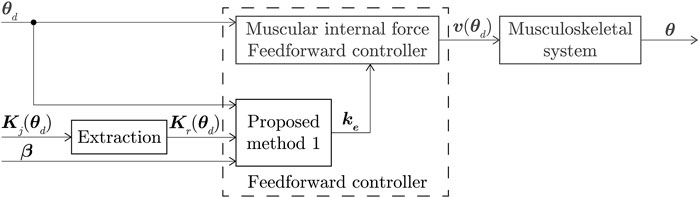
FIGURE 2. Block diagram of MIF controller using proposed Method 1.

5.1 Simulation Results

The simulated positioning control of the musculoskeletal system shown in Figure 1 was conducted to assess the ability of Method 1. This simulation shows that the MIF can eliminate the correlation between the response and stiffness at the desired position using Method 1. In these simulations, an end-point stiffness ellipsoid (Tsuji et al., 1995) was used to obtain a visual representation of the stiffness. Under this approach, the desired stiffness was represented as the end-point stiffness ${\mathit{K}}_e(\mathit{x}(\mathit{\theta }))\in {\mathbb{R}}^{2\times 2}$, and a joint stiffness K_j(θ) corresponding to the end-point stiffness was calculated. The relation between the end-point and joint stiffnesses is given by

${\mathit{K}}_j(\mathit{\theta })=\mathit{J}{(\mathit{\theta })}^{\mathrm{T}}{\mathit{K}}_e(\mathit{x}(\mathit{\theta }))\mathit{J}(\mathit{\theta }).(28)$

The MIF can be determined by substituting the elements of the desired joint stiffness, K₁₁ (θ_d), K₁₂ (θ_d), and K₂₂ (θ_d), calculated from the end-point stiffnesses K_e (x (θ_d)), respectively, into Eq. 26.

The results of positioning control using each input determined by three desired end-point stiffness matrixes K_e1 (x (θ_d)), K_e2 (x (θ_d)), and K_e3 (x (θ_d)) were compared in this simulation. The simulation employed a conventional method (CM) (Kino et al., 2013), which minimized the norm of the MIF as a comparison target. The arbitrary vector using CM is given by

${\mathit{k}}_{\mathit{e}}=\gamma {\left[\begin{array}{cccccc}\hfill 1.0\hfill & \hfill 1.0\hfill & \hfill 1.0\hfill & \hfill 1.0\hfill & \hfill 1.0\hfill & \hfill 1.0\hfill \end{array}\right]}^{\mathrm{T}}.(29)$

The result of the simulation performed by setting γ = 70 is expressed as CM1 and that for γ = 115 is expressed as CM2. Table 1 lists the physical parameters and muscular arrangements of the musculoskeletal system, respectively, and Table 2 lists the initial and desired parameters. The arbitrary vector β was set as follows:

$\mathit{\beta }=150{\left[\begin{array}{cccccc}\hfill 1.0\hfill & \hfill 1.0\hfill & \hfill 1.0\hfill & \hfill 1.0\hfill & \hfill 1.0\hfill & \hfill 1.0\hfill \end{array}\right]}^{\mathrm{T}}.(30)$

TABLE 1

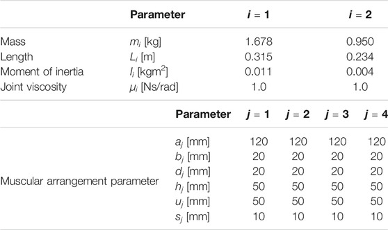
TABLE 1. Parameters of musculoskeletal system.

TABLE 2

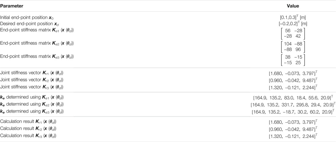
TABLE 2. Initial parameters and the results using Method 1.

Table 2 lists the values of results obtained using Method 1 as determined by Eq. 30.

The results of the simulations are shown in Figure 3 ∼ 4. Figure 3A shows the transient responses of the end-point position; Figure 3B compares the control inputs; Figure 3C ∼ Figure 3F show the end-point stiffness ellipsoids and loci of the end-point positions in the task space, respectively; Figure 4A compares the end-point stiffness ellipsoids; Figure 4B compares the end-point stiffness ellipsoids of CM2 and K_e2 (x (θ_d)); Figure 4C compares the loci of the end-point position in the task space of CM2 and K_e2 (x (θ_d)). From Figure 3A, Figure 3C ∼ Figure 3F, it is seen that the end-point positions converge at the desired position. The end-point stiffness ellipsoids corresponding to 0.1-s intervals on the end-point trajectories are shown in Figure 3C ∼ Figure 3F. In Figure 3D and Figure 3F, the major axis of the ellipsoid is shortened and the end-point trajectory bulges outward. In Figure 3E, the major axis of the ellipsoid is lengthened and the end-point trajectory suppresses the outward bulge. Although Figure 3F shows an end-point trajectory that is equivalent to the trajectory in Figure 3D, the end-point stiffness ellipsoids at the desired positions differ and the control inputs v_d3, v_d4 are significantly reduced, as shown in Figure 3B. Those results show that Method 1 can achieve low stiffness without sacrificing the response.

FIGURE 3

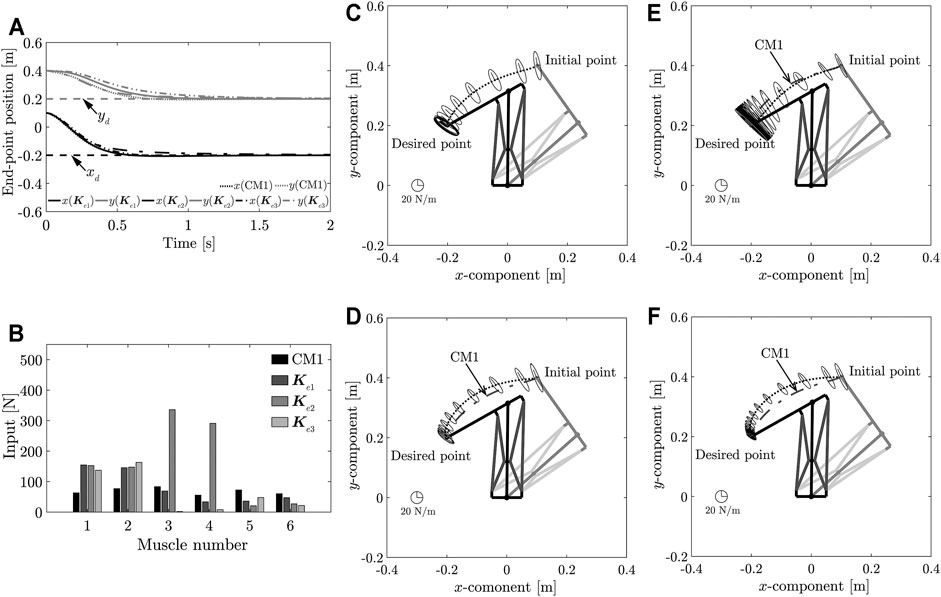
FIGURE 3. (A) Comparison of transient responses of end-point position at different desired end-point stiffnesses. (B) Comparison of control inputs. (C) Loci of end-point positions and end-point stiffness ellipsoid in the task space produced using CM1. (D) Loci of end-point positions and end-point stiffness ellipsoid in the task space produced using the stiffness matrix K_e1. (E) Loci of end-point positions and end-point stiffness ellipsoid in task space obtained using the stiffness matrix K_e2. (F) Loci of end-point positions and end-point stiffness ellipsoid in task space obtained using the stiffness matrix K_e3.

FIGURE 4

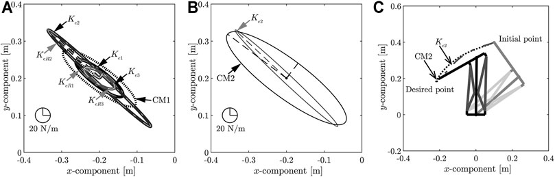
FIGURE 4. (A) Comparison of stiffness ellipsoids obtained using each desired end-point stiffness. (B)Comparison of stiffness ellipsoids obtained using the desired end-point stiffness K_e2 and CM2. (C) Comparison of loci of end-point positions at the desired end-point stiffnesses K_e2 and CM2.

A comparison of the stiffness ellipsoids K_eR1, K_eR2, K_eR3 obtained using the target end-point stiffnesses K_e1, K_e2, K_e3, respectively, is shown in Figure 4A. Figure 4A also shows the stiffness ellipsoids of CM1. In addition, joint stiffness vectors K_r which were used in determining the MIF, and joint stiffness vectors K_r which were realized by control, are shown in Table 2. These results depict that the size of the ellipsoid changed, and the desired end-point stiffness used for determining the arbitrary vector k_e was achieved. However, the ellipsoids showed almost no change in the direction of the major axis. As the direction of the major axis is dependent on the posture of the musculoskeletal system, it is difficult to have a significant impact through the controller input. However, when the arbitrary vector γ was set by constructing an end-point stiffness ellipsoid that had the same length as the major axis at the K_e2 ellipsoid, CM2 incurred an overshoot, whereas high stiffness was realized, as shown in Figure 4B and Figure 4C. Method 1 can realize high stiffness without causing an overshoot and can eliminate the correlation between the response and stiffness at the desired position.

5.2 Evaluation of End-point Stiffness Ellipsoid

The characteristics of the ellipsoid were evaluated by changing the direction of the major axis using trial and error, to uncover the relation between the end-point stiffness K_e (x (θ_d)) and axis direction, because, as discussed in the preceding section, it is difficult to significantly change the direction of the major axis of the end-point stiffness ellipsoid using control input. The stiffness matrix at the time of inputting the MIF, determined using a conventional method, was used as reference. The elements of the standardized stiffness matrix were changed to rotate the longest axis of the ellipsoid in the clockwise direction. This change was made using trial and error because the relationship between the elements and rotational direction remains unidentified. The MIF calculated based on the stiffness matrix indicates that it satisfied Eq. 12 and was less than 500. If the conditions are satisfied, same elements are changed; otherwise, other elements are modified to rotate the axis in a counter-clockwise direction. Furthermore, the axis length was not evaluated because the lengths of the major and minor axes of the ellipsoid were altered simultaneously while maintaining a constant length ratio. The response of the end-point position was also not considered.

The results of varying the direction of the major axis of the end-point stiffness ellipsoid are shown in Figure 5 and listed in Table 3. It can be observed through the results that the parameters were changed within a range at par with the norm of MIF being less than 500. Figure 5 shows the major axis direction at eight end-point positions. In addition, the end-point position x = [−0.1,0.1]^T was excluded from the evaluation because it was beyond an effective movable range. The minimum change in the angle of γ = 2.1° was attained at the position x₈ = [−0.1,0.2]^T, while the maximum change in the angle of γ = 42.8° occured at x₃ = [−0.3,0.1]^T. These results indicate that the direction of the end-point stiffness ellipsoid generated by the application of Method 1 is dependent on the posture of the musculoskeletal system. In this case, the relation between the stiffness matrix parameter K_e (x (θ_d)) and the major axis direction cannot be clarified due to position difference.

FIGURE 5

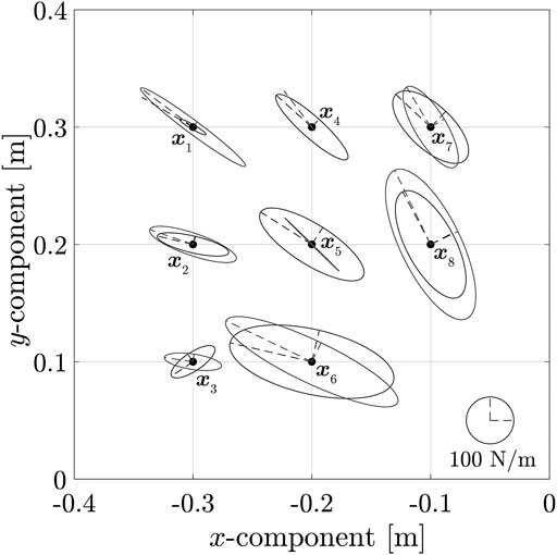
FIGURE 5. Change in orientation of major axis of ellipsoid with end-point position.

TABLE 3

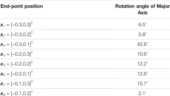
TABLE 3. Major axis of ellipsoid as a function of end-point position.

5.3 Evaluation of Modeling Error

Next, the influence of the musculoskeletal system, including modeling error, was evaluated. The modeling error that occurred during the application of Method 1 to an actual musculoskeletal system could not be ignored. However, the error was justified, as it was difficult to model the actual system accurately. Therefore, the influence of muscular arrangements, including modeling error, was evaluated. In this evaluation, it was assumed that errors in muscular arrangements occurred because of an assembly error in the musculoskeletal system. The proposed method was evaluated as a true value using the parameters listed in Table 1. The evaluation function of the end-point position and joint stiffness vector is defined as

$\begin{array}{ccc}\hfill E_e& =\hfill & \Vert {\mathit{x}}_f-{\mathit{x}}_d\Vert \hfill \end{array}(31)$

$\begin{array}{ccc}\hfill E_k& =\hfill & \Vert {\mathit{K}}_{rf}-{\mathit{K}}_r\Vert ,\hfill \end{array}(32)$

where x_f is an end-point position of a simulation finish time and K_rf is the joint stiffness vector at x_f.

One cause for the error in muscular arrangements is the assembly error of the musculoskeletal system. In this case, it was considered that large errors do not occur in the measurement values because muscular arrangements can be easily measured. Therefore, randomly selected values from a range of error rates of 5% were used as actual muscular arrangements. The MIF was determined using five muscular arrangements and three stiffness matrices, and the evaluation function was also calculated. Table 4 lists the average values of the five evaluation functions. The evaluation function of the joint stiffness vector was larger than that of the end-point. This is because the joint stiffness vector was calculated using the end-point and muscular arrangement. The evaluation function of the joint stiffness vector became larger because it was difficult to estimate the accurate joint stiffness vector when modeling errors occurred. In particular, the evaluation function of the joint stiffness vector using K_e2 (x (θ_d)) was larger than all the other values. This function synergistically became larger because the evaluation function of the end-point was larger than the other values. We propose a robust position control method for the arrangement error at this point (Matsutani et al., 2019a). A decrease in the error of the end-point position as a result of combining the proposed method with the discussed control method is expected. It was assumed that the decrease in the error of the joint stiffness vector was caused by the impact of the end-point position.

TABLE 4

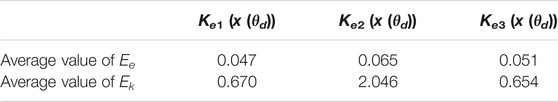
TABLE 4. Evaluation function of the end-point position and joint stiffness vector.

5.4 Evaluation of Arbitrary Vector β

We then investigated the influence of the arbitrary vector β on the control result. In this evaluation, the MIF was determined using the end-point stiffnesses K_e1 (x (θ_d)) listed in Table 2 and the arbitrary vectors β derived from Eq. 33 ∼ (Eq. 35). The simulation results obtained by applying the resulting MIFs were then compared.

$\begin{array}{ccc}\hfill {\mathit{\beta }}_1& =\hfill & 150{\left[\begin{array}{cccccc}\hfill 1.0\hfill & \hfill 1.0\hfill & \hfill 1.0\hfill & \hfill 1.0\hfill & \hfill 1.0\hfill & \hfill 1.0\hfill \end{array}\right]}^{\mathrm{T}}\hfill \end{array}(33)$

$\begin{array}{ccc}\hfill {\mathit{\beta }}_2& =\hfill & 5{\left[\begin{array}{cccccc}\hfill 1.0\hfill & \hfill 1.0\hfill & \hfill 1.0\hfill & \hfill 1.0\hfill & \hfill 1.0\hfill & \hfill 1.0\hfill \end{array}\right]}^{\mathrm{T}}\hfill \end{array}(34)$

$\begin{array}{ccc}\hfill {\mathit{\beta }}_3& =\hfill & 500{\left[\begin{array}{cccccc}\hfill 1.0\hfill & \hfill 1.0\hfill & \hfill 1.0\hfill & \hfill 1.0\hfill & \hfill 1.0\hfill & \hfill 1.0\hfill \end{array}\right]}^{\mathrm{T}}.\hfill \end{array}(35)$

Table 5 lists the arbitrary vectors k_e derived from application of Method 1, using the outputs of Eq. 33 ∼ (35); the simulation results are shown in Figure 6. Figure 6A shows the transient responses of the end-point position; Figure 6B and Table 5 compare the control inputs; Figure 6C and Figure 6D show the end-point stiffness ellipsoids and loci of end-point positions in the task space, respectively. The results obtained using the arbitrary vector β₁ were identical to those shown in Figure 3D and were therefore, not repeated. It can be observed from Figure 3D and 6 that, while the stiffness ellipsoids at the desired position were the same, the transient responses of the end-point position differed. While analyzing the changes in end-point stiffness during movement, it was observed that the ellipsoids varied significantly near the initial position, but converged completely near the desired position. This occurs because the arbitrary vector β affected only the second term of Equation 26, a term that has no effect on the end-point stiffness matrix K_e1 (x (θ_d)). This is so, because it becomes a vector that belongs to the null space of the matrix when the end-point position is the desired position. This indicates that Method 1 can be applied to change the transient responses of the end-point position, to achieve the desired end-point stiffness at the same position.

TABLE 5

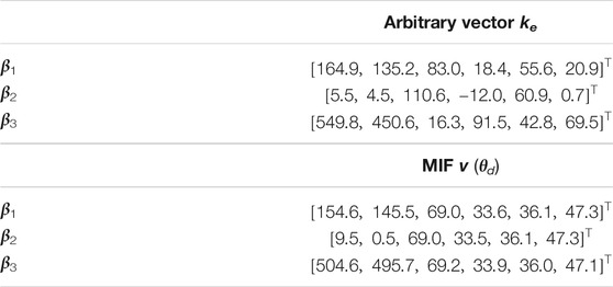
TABLE 5. Arbitrary vectors and MIFs determined mathematically using Method 1.

FIGURE 6

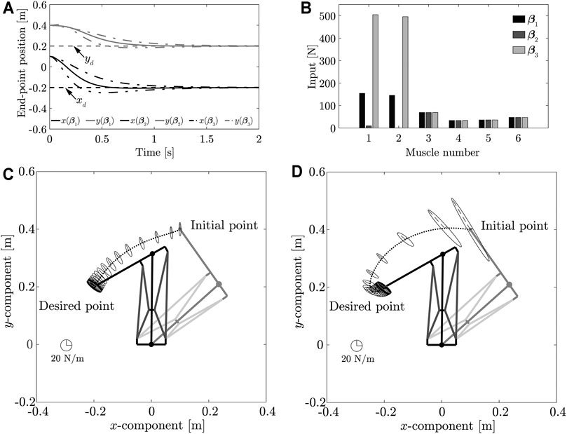
FIGURE 6. (A) Transient response of end-point position as a function of arbitrary vector value. (B) Comparison of control inputs obtained using different arbitrary vectors. (C) Loci of end-point positions and end-point stiffness ellipsoid in task space obtained using arbitrary vector β₂. (D) Loci of end-point positions and end-point stiffness ellipsoid in task space obtained using arbitrary vector β₃.

Changing the arbitrary vector β from its value in Figure 6B confirms that the arbitrary vector has no effect on the MIFs v_d3 ∼ v_d6. Similarly, changing the end-point stiffness K_e (x (θ_d)) from its value inFigure 3B confirms that this factor has no significant effect on the MIFs v_d1, v_d2. These results suggest that muscles 1, 2 contribute to the maintenance of the transient response of the end-point position while muscles 3 ∼ 6 contribute to the maintenance of end-point stiffness. However, determination of the specific roles of the muscles will require further investigation and is left as a subject for future analysis.

6 Method of Determining Muscular Internal Force Using Stiffness at the Initial and Desired Positions

In this section, a novel method for uniquely determining the MIF based on the stiffnesses at the initial and desired positions (Method 2) has been introduced. By applying Method 2, the stiffnesses at the respective positions can be controlled while performing repetitive movements. An example of this is the pick-and-place operation, in which the stiffness is set to low when the robot picks up an object, and set to high when the robot places the object.

For a balanced MIF v (θ₀) input to a muscle at the initial joint angle θ₀, the joint stiffness K_j (θ₀) at θ₀ was derived from Eq. 23 as follows:

$\left\{\begin{array}{c}{K}_{11}({\mathit{\theta }}_0)=-\frac{\partial {\mathit{w}}_a({\mathit{\theta }}_0)}{\partial {\theta }_1}\mathit{Y}({\mathit{\theta }}_0){\mathit{k}}_{\mathit{e}}\hfill \\ K_{12}({\mathit{\theta }}_0)=-\frac{\partial {\mathit{w}}_a({\mathit{\theta }}_0)}{\partial {\theta }_2}\mathit{Y}({\mathit{\theta }}_0){\mathit{k}}_{\mathit{e}}\hfill \\ K_{22}({\mathit{\theta }}_0)=-\frac{\partial {\mathit{w}}_b({\mathit{\theta }}_0)}{\partial {\theta }_2}\mathit{Y}({\mathit{\theta }}_0){\mathit{k}}_{\mathit{e}}\hfill \end{array}.\right.(36)$

Similarly, for a balance of MIFs v (θ_d) at a desired joint angle θ_d input to a muscle, the joint stiffness K_j (θ_d) at θ_d can be derived from Eq. 23 as

$\left\{\begin{array}{c}{K}_{11}({\mathit{\theta }}_d)=-\frac{\partial {\mathit{w}}_a({\mathit{\theta }}_d)}{\partial {\theta }_1}\mathit{Y}({\mathit{\theta }}_d){\mathit{k}}_{\mathit{e}}\hfill \\ K_{12}({\mathit{\theta }}_d)=-\frac{\partial {\mathit{w}}_a({\mathit{\theta }}_d)}{\partial {\theta }_2}\mathit{Y}({\mathit{\theta }}_d){\mathit{k}}_{\mathit{e}}\hfill \\ K_{22}({\mathit{\theta }}_d)=-\frac{\partial {\mathit{w}}_b({\mathit{\theta }}_d)}{\partial {\theta }_2}\mathit{Y}({\mathit{\theta }}_d){\mathit{k}}_{\mathit{e}}\hfill \end{array}.\right.(37)$

Equations 36 and 37 can be expressed in matrix form as follows:

${\mathit{K}}_u=\mathit{Q}{\mathit{k}}_{\mathit{e}},(38)$

where

$\left\{\begin{array}{c}{\mathit{K}}_u=\left[\begin{array}{c}{K}_{11}({\mathit{\theta }}_0)\hfill \\ K_{12}({\mathit{\theta }}_0)\hfill \\ K_{22}({\mathit{\theta }}_0)\hfill \\ K_{11}({\mathit{\theta }}_d)\hfill \\ K_{12}({\mathit{\theta }}_d)\hfill \\ K_{22}({\mathit{\theta }}_d)\hfill \end{array}\right]\in {\mathbb{R}}^6,\hfill \\ \mathit{Q}=\left[\begin{array}{c}-\frac{\partial {\mathit{w}}_a({\mathit{\theta }}_0)}{\partial {\theta }_1}\mathit{Y}({\mathit{\theta }}_0)\hfill \\ -\frac{\partial {\mathit{w}}_a({\mathit{\theta }}_0)}{\partial {\theta }_2}\mathit{Y}({\mathit{\theta }}_0)\hfill \\ -\frac{\partial {\mathit{w}}_b({\mathit{\theta }}_0)}{\partial {\theta }_2}\mathit{Y}({\mathit{\theta }}_0)\hfill \\ -\frac{\partial {\mathit{w}}_a({\mathit{\theta }}_d)}{\partial {\theta }_1}\mathit{Y}({\mathit{\theta }}_d)\hfill \\ -\frac{\partial {\mathit{w}}_a({\mathit{\theta }}_d)}{\partial {\theta }_2}\mathit{Y}({\mathit{\theta }}_d)\hfill \\ -\frac{\partial {\mathit{w}}_b({\mathit{\theta }}_d)}{\partial {\theta }_2}\mathit{Y}({\mathit{\theta }}_d)\hfill \end{array}\right]\in {\mathbb{R}}^{6\times 6}.\hfill \end{array}\right.(39)$

The arbitrary vector k_e can be obtained as the inverse of Eq. 38 as follows:

${\mathit{k}}_{\mathit{e}}={\mathit{Q}}^{-1}{\mathit{K}}_u.(40)$

The MIFs v (θ₀) and v (θ_d) calculated using this arbitrary vector correspond to the musculoskeletal system stiffening to values of K_j (θ₀) and K_j (θ_d) at positions θ₀ and θ_d, respectively. The application of Method 2 using the MIF controller is shown as a block diagram in Figure 7.

FIGURE 7

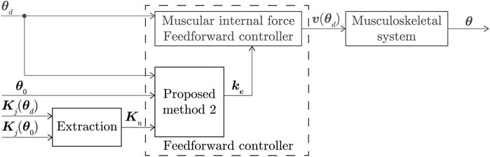
FIGURE 7. Block diagram of application of Method 2 using MIF controller.

6.1 Simulation Results

Method 2 was used to apply individual control inputs to the musculoskeletal system as it carried out repetitive movements. By changing the values of the arbitrary vector k_e, different target end-point stiffnesses were applied at various initial positions A, to serve as control inputs to the muscle for moving the system from A to a desired position B. Arbitrary values of k_e were also applied as desired end-point stiffnesses at B, using the method. The simulated positioning control of the musculoskeletal system shown in Figure 1 was conducted to evaluate the abilities of Method 2. A simulation was performed to infer that the MIF determined using Method 2, can realize the stiffness at two positions. Table 6 lists the arbitrary vector determined using Method 2 and the set of initial and desired positions, A and B, used in the simulations, respectively.

TABLE 6

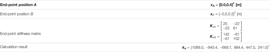
TABLE 6. Position A and B parameters and the arbitrary vector determined using Method 2.

In each simulation, the musculoskeletal system underwent controlled movement from the initial position A to the desired position B and then back from B to A. The results validated the effectiveness of Method 2 in terms of controlling the musculoskeletal system based on control of stiffness at the end-point and other positions. The physical and muscular parameters of the musculoskeletal system used in this simulation are listed in Table 1.

6.1.1 Position Control for Moving From Position A to B

Further, the position control process for motion between positions A and B was then simulated. The results of the simulation are shown in Figure 8. Figure 8A shows the end-point stiffness ellipsoids and loci of the end-point position in the task space; Figure 8B shows the transient responses of the end-point position; Figure 8C compares the respective control inputs. It can be observed from Figure 8 that the end-point position converged at the desired position x_B, and that end-point stiffness K_eB was achieved at the desired position x_B. As shown in Equation 36, a balanced MIF of v (θ_A) at the initial position was required to achieve an end-point stiffness of K_eA at this position. The end-point stiffness at the initial position x_A in Figure 8A differed from the end-point stiffness K_eA because the position control applied a balanced MIF v (θ_B) at the desired position x_B. The control input v_dl determined by Method 2 (Figure 8C) satisfied Eq. 12.

FIGURE 8

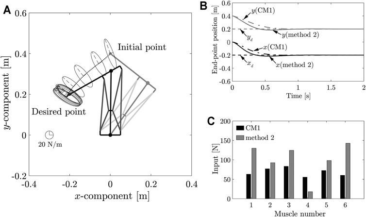
FIGURE 8. (A) Loci of end-point positions during movement from positions A to B, and end-point stiffness ellipsoids in task space. (B) Transient response of end-point position during movement from position A to position B. (C) Control input using MIF balancing at position A.

6.1.2 Position Control for Moving From Position B to A

We then simulated position control for the movement from position B to A. The results of this simulation are shown in Figure 9. Figure 9A shows the end-point stiffness ellipsoids and loci of the end-point positions in the task space. Figure 9B shows the transient responses of the end-point position. While, Figure 9C compares the control inputs. It can be observed from Figure 9 that the end-point position converged at the desired position x_A and that an end-point stiffness K_eA was achieved at the desired position. The control input determined by applying Method 2 (Figure 9C) satisfied Eq. 12. The results in this section and the preceding one demonstrate that Method 2 can be applied to uniquely determine the MIF. It is difficult to significantly alter the direction of the major axis of the end-point stiffness ellipsoid using the control input because the end-point stiffness depends on the posture of the musculoskeletal system. However, this method can still be used to control the end-point stiffnesses at the two positions effectively. In this study, the control input can be uniquely determined using Method 2 because the control target is a two-link system with six muscles. If Method 2 were used in a system with a greater number of redundancies, it would not be possible to determine the control input uniquely. Meanwhile, it was considered to increase the selectable range of the direction of the end-point stiffness ellipsoid. In addition, the control input can be uniquely determined by setting subtasks according to the redundancies in this case.

FIGURE 9

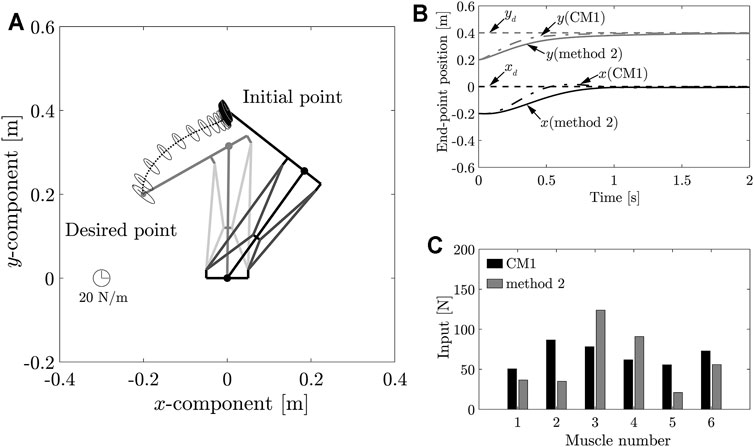
FIGURE 9. (A) Loci of end-point positions during movement from positions B to A and end-point stiffness ellipsoids in task space. (B) Transient response of end-point position during movement from position B to position A. (C) Control input using MIF balancing at position A.

7 Conclusion

In this study, two new methods for determining MIF using joint stiffness were developed, to solve the issues in a previously developed musculoskeletal system MIF feedforward controller. Using the first method (Method 1), a MIF that eliminates the correlation between the response and stiffness at a desired position was determined. Using the second method (Method 2), an arbitrary vector that reflects the stiffnesses at the initial and desired positions was determined, and applied to uniquely determine the balance of MIFs at each position. Although it was found to be difficult to significantly alter the stiffness using the control input, as the end-point stiffness depends on the posture of the musculoskeletal system, we believe that the proposed system can be adapted to expand the region of feasible stiffness control (Matsutani et al., 2017); and this will be a subject of our future analysis. The proposed methods can realize sensorless position and stiffness control. In addition, by combining the existing control method with the proposed method, runaway of movement at sensor crashes can be prevented. Further, we plan to experimentally verify this in a future study.

Furthermore, the MIF is expected to be combined with feedback control in a future work. This paper describes the evaluation of the musculoskeletal system, including the modeling error. Feedforward control is incapable of handling unanticipated contact. A combination of the MIF and feedback control complement each other to improve accuracy. For example, a stable region of feedback control that tends to become unstable can be assured by combining feedforward control based on the potential no needing an inverse dynamics model (Matsutani et al., 2018). In future works, this combination needs to be discussed in detail.

Data Availability Statement

The original contributions presented in the study are included in the article/Supplementary Material, further inquiries can be directed to the corresponding author.

Author Contributions

YM contributed to the proposed method, simulations, analysis and wrote the manuscript. KT and HK supervised the research. All authors read and approved the final manuscript.

Funding

This work was supported by JSPS KAKENHI Grant Number JP19K20378 and the Nagamori Foundation.

Conflict of Interest

The authors declare that the research was conducted in the absence of any commercial or financial relationships that could be construed as a potential conflict of interest.

Publisher’s Note

All claims expressed in this article are solely those of the authors and do not necessarily represent those of their affiliated organizations, or those of the publisher, the editors and the reviewers. Any product that may be evaluated in this article, or claim that may be made by its manufacturer, is not guaranteed or endorsed by the publisher.

References

Albu-Schaffer, A., Ott, C., Frese, U., and Hirzinger, G. (2003). “Cartesian Impedance Control of Redundant Robots Recent Results with the Dlr-Light-Weight-Arms,” in Proc. 2003 IEEE Int. Conf. on Robotics and Automation, Taipei, Taiwan, September 14–19, 2003, 3704–3709.

Google Scholar

Asano, Y., Nakashima, S., Kozuki, T., Ookubo, S., Yanokura, I., Kakiuchi, Y., et al. (2016). “Human Mimetic Foot Structure with Multi-Dofs Nad Multi-Sensors for Musculoskeletal Humanoid Kengoro,” in Proc. 2016 IEEE/RSJ Int. Conf. on Intelligent Robots and Systems, Daejeon, Korea, October 9–14, 2016, 2419–2424.

Google Scholar

Baillieul, J. (1986). “Avoiding Obstacles and Resolving Kinematic Redundancy,” in Proc. 1986 IEEE Int. Conf. on Robotics and Automation, San Francisco, CA, April 7–10, 1986, 1698–1704.

Google Scholar

Behzadipour, S., and Khajepour, A. (2006). Stiffness of cable-based Parallel Manipulators with Application to Stability Analysis. Jour. Mech. Des. 128, 303–310. doi:10.1115/1.2114890

CrossRef Full Text | Google Scholar

Buchler, D., Calandra, R., Scholkopf, B., and Peters, J. (2018). Control of Musculoskeletal Systems Using Learned Dynamics Models. IEEE Robot. Autom. Lett. 3, 3161–3168. doi:10.1109/LRA.2018.2849601

CrossRef Full Text | Google Scholar

Chirikjian, G. S., and Burdick, J. W. (1990). “An Obstacle Avoidance Algorithm for Hyper-Redundant Manipulators,” in Proc. IEEE Int. Conf. on Robotics and Automation, Cincinnati, OH, May 13–18, 1990, 625–631.

Google Scholar

Hanafusa, H., Yoshikawa, T., and Nakamura, Y. (1981). “Analysis and Control of Articulated Robot Arms with Redundancy,” in Proc. 8th IFAC World Congress, Kyoto, Japan, August 24–28, 1981, 78–83. doi:10.1016/s1474-6670(17)63754-6

CrossRef Full Text | Google Scholar

Jantsch, M., Schmaler, C., Wittmeier, S., Dalamagkidis, K., and Knoll, A. (2011). “A Scalable Joint-Space Controller for Musculoskeletal Robots with Spherical Joints,” in Proc. 2011 IEEE Int. Conf. on Robotics and Biomimetics, Karon Beach, Thailand, December 7–11, 2011, 2211–2216. doi:10.1109/robio.2011.6181620

CrossRef Full Text | Google Scholar

Katayama, M., and Kawato, M. (1990). “Learning Trajectory and Force Control of an Artificial Muscle Arm by Parallel-Hierarchical Neural Network Model,” in Proc. 1990 conference on Advances in neural information processing systems 3, Denver, Colorado, November 26–29, 1990, 436–442.

Google Scholar

Kino, H., Kikuchi, S., Matsutani, Y., Tahara, K., and Nishiyama, T. (2013). Numerical Analysis of Feedforward Position Control for Non-pulley Musculoskeletal System: a Case Study of Muscular Arrangements of a Two-Link Planar System with Six Muscles. Adv. Robotics 27, 1235–1248. doi:10.1080/01691864.2013.824133

CrossRef Full Text | Google Scholar

Kino, H., Kikuchi, S., Yahiro, T., and Tahara, K. (2009). “Basic Study of Biarticular Muscle’s Effect on Muscular Internal Force Control Based on Physiological Hypotheses,” in Proc. 2009 IEEE Int. Conf. on Robotics and Automation, Kobe, Japan, May 12–17, 2009, 4195–4200. doi:10.1109/robot.2009.5152196

CrossRef Full Text | Google Scholar

Kino, H., Ochi, H., Matsutani, Y., and Tahara, K. (2017). Sensorless point-to-point Control for a Musculoskeletal Tendon-Driven Manipulator: Analysis of a Two-Dof Planar System with Six Tendons. Adv. Robotics 31, 851–864. doi:10.1080/01691864.2017.1372212

CrossRef Full Text | Google Scholar

Klein, C. A., and Huang, C.-H. (1983). Review of Pseudoinverse Control for Use with Kinematically Redundant Manipulators. IEEE Trans. Syst. Man. Cybern. SMC-13, 245–250. doi:10.1109/TSMC.1983.6313123

CrossRef Full Text | Google Scholar

Marques, H. G., Jantsch, M., Wittmeier, S., Holland, O., Alessandro, C., Diamond, A., et al. (2010). “Ecce1: The First of a Series of Anthropomimetic Musculoskeletal Upper Torsos,” in Proc. 10th IEEE-RAS Int. Conf. on Humanoid Robots, Nashville, TN, December 6–8, 2010, 391–396. doi:10.1109/ichr.2010.5686344

CrossRef Full Text | Google Scholar

Matsutani, Y., Tahara, K., Kino, H., and Ochi, H. (2018). Complementary Compound Set-point Control by Combining Muscular Internal Force Feedforward Control and Sensory Feedback Control Including a Time Delay. Adv. Robotics 32, 411–425. doi:10.1080/01691864.2018.1453375

CrossRef Full Text | Google Scholar

Matsutani, Y., Tahara, K., Kino, H., and Ochi, H. (2017). “Stiffness Evaluation of a Tendon-Driven Robot with Variable Joint Stiffness Mechanisms,” in Proc. IEEE-RAS 17th Int. Conf. on Humanoid Robotics, Birmingham, United Kingdom, November 15–17, 2017, 213–218. doi:10.1109/humanoids.2017.8246877

CrossRef Full Text | Google Scholar

Matsutani, Y., Tahara, K., and Kino, H. (2019a). “Robust Position Control Method for Wire Arrangement Error of Tendon-Driven Robot,” in Proc. JSME annual Conference on Robotics and Mechatronics, Hiroshima, Japan, June 5–8, 2019, 1A1–S01. in Japanese. doi:10.1299/jsmermd.2019.1a1-s01Robomech2019

CrossRef Full Text | Google Scholar

Matsutani, Y., Tahara, K., and Kino, H. (2019b). Set-point Control of a Musculoskeletal System under Gravity by a Combination of Feed-Forward and Feedback Manners Considering Output Limitation of Muscular Forces. J. Robot. Mechatron. 31, 612–620. doi:10.20965/jrm.2019.p0612

CrossRef Full Text | Google Scholar

Mayorga, R. V., and Wong, A. K. C. (1988). “A Singularities Avoidance Approach for the Optimal Local Path Generation of Redundant Manipulators,” in Proc. 1988 IEEE Int. Conf. on Robotics and Automation, Philadelphia, PA, April 24–29, 1988, 49–54.

Google Scholar

Mizuuchi, I., Yoshikai, T., Sodeyama, Y., Nakanishi, Y., Miyadera, A., Yamamoto, T., et al. (2006). “Development of Musculoskeletal Humanoid Kotaro,” in Proc. 2006 IEEE Int. Conf. on Robotics and Automation, Orlando, FL, May 15–19, 2006, 82–87.

Google Scholar

Nakamura, Y., and Hanafusa, H. (1987). Optimal Redundancy Control of Robot Manipulators. Int. J. Robotics Res. 6, 32–42. doi:10.1177/027836498700600103

CrossRef Full Text | Google Scholar

Nakiri, D., and Kino, H. (2009). “Application of Cylindrical Elastic Elements for Stiffness Control of Tendon-Driven Manipulator and Inverse Kinematics Evaluation,” in Proc. 3rd Int. Conf. on Complex, Intelligent, and Software Intensive Systems, 1217–1222. doi:10.1109/cisis.2009.68

CrossRef Full Text | Google Scholar

Niiyama, R., Nagakubo, A., and Kuniyoshi, Y. (2007). “Mowgli: a Bipedal Jumping and landing Robot with an Artificial Musculoskeletal System,” in Proc. 2007 IEEE Int. Conf. on Robotics and Automation, Rome, Italy, April 10–14, 2007, 2546–2551. doi:10.1109/robot.2007.363848

CrossRef Full Text | Google Scholar

Niiyama, R., Nishikawa, S., and Kuniyoshi, Y. (2012). Biomechanical Approach to Open-Loop Bipedal Running with a Musculoskeletal Athlete Robot. Adv. Robotics 26, 383–398. doi:10.1163/156855311X614635

CrossRef Full Text | Google Scholar

Shimizu, M., Kakuya, H., Yoon, W.-K., Kitagaki, K., and Kosuge, K. (2008). Analytical Inverse Kinematic Computation for 7-dof Redundant Manipulators with Joint Limits and its Application to Redundancy Resolution. IEEE Trans. Robot. 24, 1131–1142. doi:10.1109/TRO.2008.2003266

CrossRef Full Text | Google Scholar

Suh, K. C., and Hollerbach, J. M. (1987). “Local versus Global Torque Optimization of Redundant Manipulators,” in Proc. 1987 IEEE Int. Conf. on Robotics and Automation, Raleigh, NC, March 31–April 3, 1987, 619–624.

Google Scholar

Sui, C., and Zhao, M. (2004). “Control of a 3-dof Parallel Wire Driven Stiffness-Variable Manipulator,” in Proc. 2004 IEEE Int. Conf. on Robotics and Biomimetics, , Shenyang, China, August 22–26, 2004, 204–209.

Google Scholar

Svinin, M. M., Hosoe, S., Uchiyama, M., and Luo, Z. W. (2002). “On the Stiffness and Stiffness Control of Redundant Manipulators,” in Proc. 2002 IEEE Int. Conf. on Robotics and Automation, Washington, DC, May 11–15, 2002, 2393–2399.

Google Scholar

Tsuji, T., Morasso, P. G., Goto, K., and Ito, K. (1995). Human Hand Impedance Characteristics during Maintained Posture. Biol. Cybern. 72, 475–485. doi:10.1007/BF00199890

PubMed Abstract | CrossRef Full Text | Google Scholar

Verrelst, B. r., Ham, R. V., Vanderborght, B., Daerden, F., Lefeber, D., and Vermeulen, J. (2005). The Pneumatic Biped ?Lucy? Actuated with Pleated Pneumatic Artificial Muscles. Auton. Robot 18, 201–213. doi:10.1007/s10514-005-0726-x

CrossRef Full Text | Google Scholar

Viau, J., Chouinard, P., Bigue, J.-P. L., Julio, G., Michaud, F., Shimoda, S., et al. (2015). “Projected Pid Controller for Tendon-Driven Manipulators Actuated by Magneto-Rheological Clutches,” in Proc. 2015 IEEE/RSJ Int. Conf. on Intelligent Robots and Systems, Hamburg, Germany, September 28–October 2, 2015, 5954–5959. doi:10.1109/iros.2015.7354224

CrossRef Full Text | Google Scholar

Yoshikawa, T. (1985). “Manipulability and Redundancy Control of Robotic Mechanisms,” in Proc. 1985 IEEE Int. Conf. on Robotics and Automation, St. Louis, MO, March 25–28, 1985, 1004–1009.

Google Scholar