Convolutional Neural Network for Driving Maneuver Identification Based on Inertial Measurement Unit (IMU) and Global Positioning System (GPS)

Introduction

Since the number of vehicles and road traffic users are increasing rapidly, the number of accidents is also increasing. In everyday life, car drivers are involved in several driving maneuver e.g., driving in roundabouts, left and right turns, breaks, etc. while they are driving, and risky maneuver are also causing accidents (Gerdes, 2006). Thus, road traffic safety issues are increasingly important for research and development for governments and vehicles manufacture. The European Commission is aiming to reduce the number of road accidents with the vision to achieve zero road fatalities in EU (KPMG, 2012; Fagnant and Kockelman, 2013). To meet this objective and to improve the traffic safety and efficiency, it is necessary to understand the wide variety of styles for driving maneuver which promotes initiatives to conduct researches to reduce the rate of road accidents and to improve road safety. Again, understanding the driving maneuver can help us to build models of drivers to improve Advanced Driver Assistance Systems (ADASs), vehicle safety, and privacy and help to detect risky driving styles (Zardosht et al., 2018).

“SimuSafe: Simulation of behavioral aspects for safer transport” is a project funded by the European Union, H2020, where one of the main objectives is to create a realistic behavioral model such that researchers will be able to conduct research and collect data not available in real-world circumstances (Ahmed et al., 2017). Under the SimuSafe project, Naturalistic Driving Studies (NDS) have been conducted to examine a real traffic situation by observing the drivers driving maneuver like accidents and near misses, crashes, etc. (Barnard et al., 2016; Muronga, 2017; Feng, 2019). As NDS data are collected along with a large time frame this makes the time-consuming, tedious and impractical task of identifying maneuver manually by a human. Thus, this challenge has inspired the need to research and develop an automated system that capable of identifying potential maneuver i.e., roundabouts reliably. Several research studies have been found in the literature that aim for identification of basic events, e.g., identify whether a car is accelerated, braked, made a left/right/U-turns, or any risky driving maneuver, e.g., sharp turning (Di Lecce and Calabrese, 2009; Johnson and Trivedi, 2011; Van Ly et al., 2013; Zheng and Hansen, 2016; Hernández Sánchez et al., 2018; Ouyang et al., 2018; Ma et al., 2019), however, the identification of roundabouts is not as common (Zhao et al., 2017; Altarabichi et al., 2019).

The main challenge in this study is to determine the best Machine Learning (ML) algorithm for identifying driving maneuver i.e., roundabouts from the NDS based on the sensory data from IMU and GPS by investigating several ML algorithms. This paper presents an automatic driving maneuver e.g., driving in roundabouts, left and right turns, breaks, etc. identification system. Here, the study determines Convolutional Neural Network (CNN) as a best ML algorithm to identify driving maneuver based on Inertia Measurement Unit (IMU) and Global Positioning System (GPS) data collected through the NDS in SimuSafe. The proposed system is also compared and evaluated with different ML algorithms e.g., Hidden Markov Model (HMM), Random Forest (RF), Artificial Neural Network (ANN), K-nearest neighbor (k-NN) and Support Vector Machine (SVM) to observe the capability of detecting driving maneuver, specifically the driving maneuver for navigating a roundabout. The NDS data are collected using 16 volunteers over a period of 3 months in two different countries through naturalistic driving, i.e., the drivers were not controlled and restricted to a predetermined path. Here, the test cars were equipped with GPS and IMU, and the IMU consists of an accelerometer and a gyroscope. Thus, the test vehicular sensors are used to capture different aspects of driving dynamics and motion to identify roundabout as a driving maneuver.

Background and Related Work

ML is a subset of AI focuses on developing computer programs capable of learning from experience (Fernandes de Mello and Antonelli Ponti, 2018). According to –Tom Mitchell, “a computer program is said to learn from experience E with respect to some class of tasks T and performance measure P if its performance at tasks in T, as measured by P, improves with experience E” (Robert, 2014). Supervised classification problems involve an input space (i.e., the instances of χ) and an output space (e.g., the labeling of Υ). An unknown target function f:χ → Υ defines the functional relationship between the input space and output space. As mentioned above, a dataset D exists containing input-output pairs (χ₁, Υ₁), ……, (χ_n, Υ_n) drawn as an independent and identical distribution (i.i.d) from an unknown underlying distribution P(χ, Υ). The goal is to find a function g:χ → Υ that can approximate the solution of f with minimum errors. The function g:χ → Υ is called a classifier (Friedman et al., 2001). Supervised learning is applicable when the given set of data has a known output for the specified inputs. Several supervised ML algorithms i.e., CNN, ANN, HMM, RF, k-NN, and SVM.

The HMM is a supervised learning algorithm, widely used for classification and pattern recognition. It has been used in the field of voice recognition to determine the phrase or word and in the context of natural language processing (NLP), i.e., part-of-speech tagging and noun-phrase chunking (Rabiner, 1989). HMM is built on the assumption that only the results of the actions of states are observable, states are not directly observable, they make observations, which are weighted by their probability. By considering all the possible order of states, and the probability of their actions, the order of states that has the highest probability is selected as the final one. Two models are currently considered namely, Discrete Hidden Markov Models (DHMMs) and Continuous Hidden Markov Models (CHMMs) (Attal et al., 2013; Yiyan et al., 2017).

k-NN is a non-parametric simplistic ML algorithm. It does not need to fit the data, which makes it flexible in the sense that k-NN is a memory-based algorithm which uses the observations in the training set to find the most similar properties of the test dataset (Breiman, 2001). In other words, k-NN classifies an unseen instance using the observations that have closest match similarity (k-number nearest neighbors) to it. In the statistical settings, k-NN does not make any assumptions about the underlying joint probability density, rather uses the data to estimate the density. In k-NN, a distance function e.g., the Euclidean distance function is often used to find the k most similar instances. Then methods like majority voting is used on the k-neighbor instaces that indicates most commonly occurring classification to make the final classification. The bias-variance trade-off of k-NN depends of the selection of k, i.e., the number of nearest neighbors to be considered. As the value of k gets larger the estimation smoothed out more. Since k-NN is based on a distance function, it is straightforward to explain the nearest-neighbor model when predicting a new unseen data. However, it may be difficult to explain what inherent knowledge the model has learned.

ANN is a method that is vaguely inspired by the biological nervous system, i.e., neurons in a brain. It is composed of interconnected elements called neurons that work in unity to solve specific problems (Basheer and Hajmeer, 2000; Drew and Monson, 2000; Zhang, 2000). The neurons are connected through links, and numerical weight is assigned to each neuron. This weight represents the strength or importance of each neuron input and repeated adjustment of the weights are performed to learn from the input. Various types of neural networks are described in Basheer and Hajmeer (2000), and one of the most popular network architectures is the multilayer feedforward neural network methods using backpropagation to adapt/learn the weights and biases of the nodes. Such networks consist of an input layer that represents the input variables to the problem, an output layer consisting of nodes representing the dependent variables or the classification label, and one or more hidden layers that contain nodes to help capturing the nonlinearity of the data. The error is computed at the output layer and propagates backwards from the output layer to the hidden layer, then hidden layer to the input layer.

CNN is the most common approach that uses deep learning that applies neural network architectures with more than one hidden layer, i.e., if there are multiple hidden layers, it is referred to as a Deep Neural Network (DNN). One of the most popular types of deep neural networks is known as CNN and commonly used for pattern recognition and image processing, such as street sign recognition and pedestrian detection (Gerdes, 2006; Zhao et al., 2017). Like a typical neural network, a CNN consists of an input layer, a combination of convolutional and pooling layers, i.e., has neurons with weights and biases. The model learns these values during the training process, and it continually updates them with each new training example. However, in the case of CNNs, the weight and bias values are the same for all the hidden neurons in a given layer. The advantages of using CNN is that it requires less or no prepossessing (Al-luhaibi et al., 2018), a graphical representation can be seen in Figure 1.

FIGURE 1

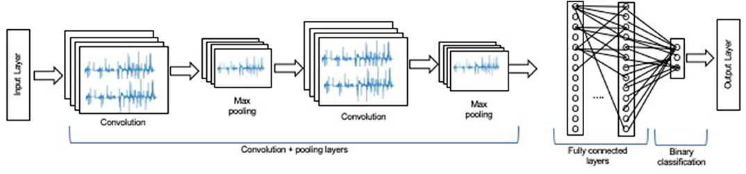
Figure 1. A graphical representation of CNN is presented.

RF is a popular ensemble algorithm in ML that consists of a series of randomized decision trees, where every tree is built using a random split selection (Breiman, 2001). Each decision tree is trained using bootstrap data samples, where bootstrapping is the process of creating samples with replacement. During the bootstrapping process, not all the data are selected for training; the selected data are referred to as out-of-bag data, and these out-of-bag data are used to find the generalization error or the out-of-bag error. The trees will each have a random bias, to not overfit the data. During the tree-generation process, for the k-th tree, a random vector υ_k is generated, which is drawn from the same data distribution but independent of previous random vectors υ₁, ……, υ_k−1. For the given training dataset, the tree grows using the random vectors υ_k and creates a predictor h(χ, X_k, υ_k), where χ is the input data, X_k is the bootstrap sample, and υ_k consists of several number of independent random variables m between 1 and K. Different generalizations can be achieved by varying the number of variables; it is recommended to start the search from m = [log₂ K+1] or $m=\sqrt{K}$ (Breiman, 1996, 2001). After generating a large number of trees, the output is the majority vote of all these decision trees. The important aspects of a random forest are that as the forest grows by adding more trees, it will converge to a limiting value that reduces the risk of overfitting and does not assume feature independence. RF is implemented using bagging, which is the process of bootstrapping the data plus using aggregation to make a decision. Thus, from a given input, the algorithm selects the most common class from the collection of trees to be the best choice (Vapnik, 1992; Ho, 1995).

SVM is used for separating and classifying data into different distinct classes by finding the hyperplane that not only minimizes the empirical classification error but also maximizes the geometric margin of the classification (Vapnik, 1992; Guyon et al., 2002). SVM maps the original data points in the input space to a high dimensional feature space, making the classification problem simpler. Hence, SVM is suitable for classification problems with redundant datasets (Ertel, 2018). Consider an n-class classification problem with a training data set ${\left\{{\chi }_i,{{\rm Y}}_i\right\}}_{i=1}^n$, where ${\chi }_i\in {ℝ}^{\text{d}}$ is the input vector, and Υ_i is the corresponding class label. The SVM maps the d-dimensional input vector space to a d_h-dimensional feature space and learns the separating hyperplane 〈w, χ〉+b = 0, b∈ℝ that maximizes the margin distance $\frac{2}{\left|\right|w|{|}_2^2}$, where w is a weight vector, and b is the bias. The SVM classifier obtains a new label $\widehat{{\rm Y}}$ for the test vector by evaluating Equation (1):

$\begin{array}{ll}\widehat{{\rm Y}}={\displaystyle \sum _{i=1}^N}{w}_i.K(\chi ,{\chi }_i)+b& (1)\end{array}$

where N is the number of support vectors, w_i are the weights, b is the bias that is maximized during training and K is the kernel function.

An overview of different ML approaches in driving maneuver identification with a result analysis of the related work is presented in Table 1. As can be seen accelerometer, gyroscope, magnetometer is commonly used as IMU together with GPS. These parameters are gathered through smart phones, car CANbus, and other specific devices. Again, commonly used ML algorithms are ANN, RF, k-NN, LR, and SVM. Here, all of them are supervised ML algorithms, which includes classes between two and twelve, e.g., stop and start maneuver, and turns, aggressive turns, U-turns, aggressive U-turns, aggressive acceleration, aggressive braking, swerve, device removal, excessive Speed. It was also observed that several of the research has identified maneuver with a higher accuracy i.e., more than 90% accuracy. For example, the authors in Zheng and Hansen (2016) applied SVM, and Topology anomaly detection for driver behavior based on accelerometer, gyroscope and GPS through smart phone. Again, in our previous work (Altarabichi et al., 2019) and (Larose, 2005), several ML algorithms such as ANN, RF, k-NN, LR, SVM have been applied in IMU and 3-D sensors that had been mounted in a car and motorcycle to classify roundabouts, left turns, right turns, straights, and stops. Unsupervised ML such as PCA, CNN and RNN have also been applied on accelerometer data collected from the car to classify accelerations, breakings, and turns as presented in Hernández Sánchez et al. (2018). Different anomaly detection algorithms were compared by Ma et al. (2019) to detect aggressive behavior of the drivers using motion data from an accelerometer and gyroscope data that are collected by a smartphone mounted in a vehicle. The algorithms have used in the report are Gaussian Mixture Model (GMM), Partial Least Squares Regression (PLSR), Wavelet, and SVR. SVR is a regression version of SVM. Their results have shown that the algorithms are promising for detecting aggressive driving when using both the accelerometer and gyroscope, compared to when using either of the sensors independently. The GMM got a F₁-score of 0.76 and SVR got 0.73.

TABLE 1

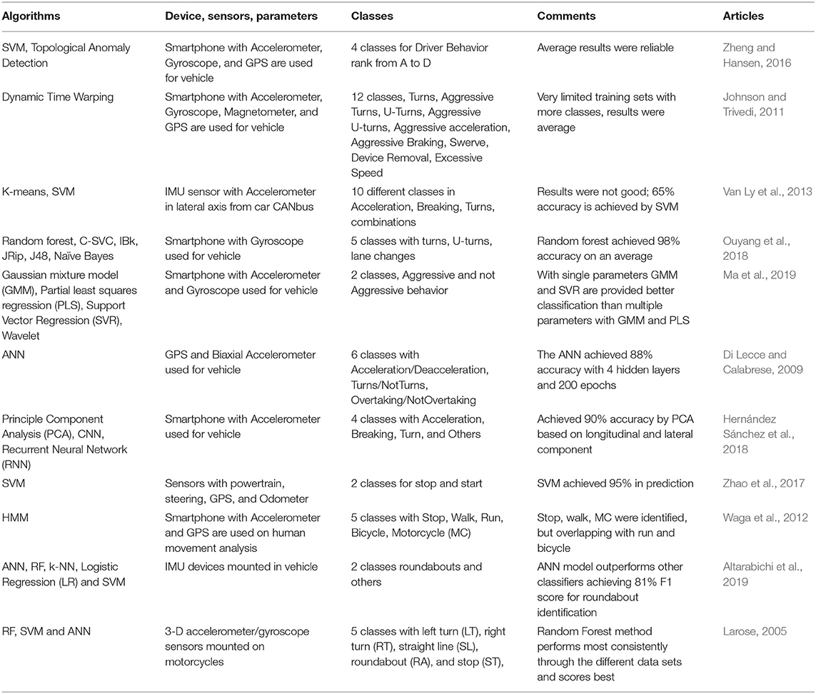
Table 1. Some related articles based on ML algorithms, parameters, sensors, etc.

Materials and Methods

The data used in this study are obtained through the SIMUSAFE project using timestamped sensor data that corresponds to NDS trips. There are 16 volunteers and the data are collected between May and August 2018. The data had been collected from cars equipped with sensors, e.g., the IMU and GPS.

Inertial measurement unit (IMU) is required within SIMUSAFE DAS because such measurements available on-board in vehicles are not standardized. Thus, myAHRS+ is used as exact unit because of its guaranteed compatibility with ODROID DCP. Another important advantage is the availability of a driver (BSD license) for ROS distribution used in SIMUSAFE DCP. The IMU requires calibration due to installation position, because measurements in host vehicle coordinate system are required. Similarly, a USB GPS module named “Ublox G7020-KT” is used because of cost and being distributed over ODROID website, thus ensuring compatibility and support of the SIMUSAFE DCP. The GPS unit readings are handled by DCP system that uses a gpsd service. Such system was found not to provide a PPS signal and therefore DCP clock is synchronized over network rather than via GPS. The roundabout entries from the smart camera were used to label the datasets to find out whether they are roundabout or not. The GPS is used to collect the longitudinal and latitudinal coordinates. Since the supervised learning requires data to be labeled, all the GPS points were plotted on a map as presented in Figure 2. Two types of feature extractions have been conducted, (1) window-based feature extraction and (2) maneuver-based feature extraction. Here, the fixed window-based feature extraction is more common, widely used traditional approach where the sample size can be increased and decreased based on the size of the window and also, calculation time is very less. As the window size is always same for all the feature, the feature value is stable. On the other hand, the maneuver-based is a new way to test the approach, proposed by Pilko et al. (2014) and Gonzalez et al. (2017), here the concept of dividing the driving process in a roundabout into three stages: entrance, driving within the roundabout and exit maneuvers. To account for this maneuvers sequence, each dataset instance is built using a rolling window with three maneuvers as a window size. Thus, the sample size is decreased and also feature value is not stable and window size is different for each feature as it is depending on the combination of a sequence entrance -> in the roundabout -> exit. Moreover, the computation time is also very high then the other method and as the sample size it less no possibility to used CNN.

FIGURE 2

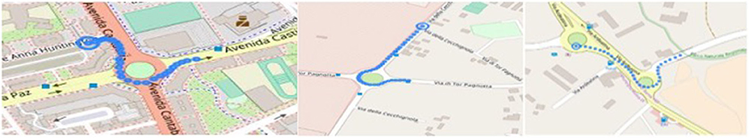
Figure 2. Example of roundabout labeled by GPS data.

In window-based feature extraction, the roundabout detection model is developed to use IMU sensor data for the purpose of classification, eight signals are utilized from IMU sensory data as observed in Table 2. The IMU sensors collected data in the form of acceleration in the longitude, lateral, and vertical direction, pitch, roll values, and yaw rate. The longitude axis was aligned with the direction of the car face, and the vertical axis was placed perpendicular to the road (Altarabichi et al., 2019). The filtered and labeled data set contains 76306 data points, of which 847 are labeled as roundabouts. The calculated median time to travel through a roundabout, in the data set, is 8 s, with the average time being slightly longer. The data are windowed, windowing gives information before and after a given point and therefore aids the classification of longer lasting maneuver.

TABLE 2

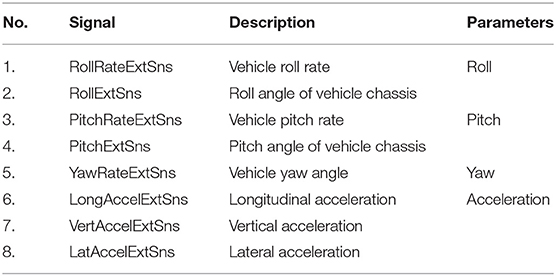
Table 2. IMU sensor signals with corresponding parameters.

In maneuver-based feature extraction, the data are resampled with 14 to 1 Hz to reduce signal noise, and a Gaussian rolling window is applied to smoothen the resampled signals. The YawRateExtSns is selected as a base signal to establish the start and end time of driving maneuvers. The integral of YawRateExtSns readings between start and end time is calculated to measure the corresponding Yaw angle of the performed maneuver. The time series of sensor readings that represent driving trip is transformed accordingly into a sequence of maneuvers performed by the vehicle. Driving maneuvers are presented by eight time-domain features that correspond to the mean value of each of the eight IMU signals throughout the maneuver. A ninth feature is added that corresponds to the calculated Yaw angle, and a feature that corresponds to the duration of the maneuver in seconds is added to total of 10 features per maneuver. This approach generated a training data set that consist of 22111 instances. GPS signals were used to label 249 roundabouts occurrences manually according to the map images of the driving trips (Altarabichi et al., 2019).

With window-based features, the CNN, HMM, RF, and SVM have been applied to classify maneuver. In our previous work (Altarabichi et al., 2019), the class imbalance in the dataset is addressed by performing validation assigning a weight to roundabout class {1, 2, 4, 8, 16, 99}, however, the results were not satisfactory. Thus, the paper focuses both on assigning a weight to roundabout class and the stratified sampling on the imbalance data set for the machine learning modeling. Through CNN, to account for the unbalanced representation of classes, roundabouts are given a class-weight of 4 : 1. The data were windowed and split into a training and a test set using stratified sampling. The stratified split makes sure both the sets had the same class representation. The CNN is trained using the 10-fold cross-validation. The model with the lowest categorical cross-entropy validation loss is used for the evaluation of the test data set. The implementation of the CNN algorithm is conducted using Python Deep Learning library Keras², here, the parameters are presented in Tables 3, 4. For HMM, the models are created with the 4 states and trained using the Baum-Welsh algorithm (Li and Jain, 2009). Here, the number of the states are determined through manual testing by evaluating the accuracy. To avoid getting stuck in a local optimum, different initialization is used. The models with different initialization are compared based on the log probability of the training data, and the best one is selected. Also, windowing is used on the testing data with a window size of 7 and a stride of 1. The window size is determined manually by evaluating the accuracy. The implementation is conducted through the hidden Markov model module simplehmm.py provided with the Febrl system is a modified re-implementation of LogiLab's Python HMM module³. The evaluation is done using 10-fold cross validation based on the IMU signals, to get an average accuracy and to prevent the accuracy from being biased. For RF, the hyperparameters are selected based on the directed grid search with cross-validation. The data are windowed, standardized, and 10-fold cross validation is used here. The parameters are window size =9, estimators=100, criterion = entropy, class weight = balanced, max features = sqrt, min sample split = 25 and min samples leaf = 1 through the python programming and using scikit-learn library⁴. For k-NN, classifier k=1 is considered while using Python Scikit-learn package library⁴. Here, import the KNeighborsClassifier module is used to construct the model together with fit() function as training and predict() function as test. For the dataset splitting the function train_test_split() is used with 3 parameters features, target, and test_set size. For SVM, different kernel function has been used such as Radial Basis Function (RBF), sigmoid and polynomial. To find hyperparameters, grid search is used on arbitrarily selected parameters with a large range on a limited data set. Grid search could have been used as a key tool to find suitable parameters for different classification models.

TABLE 3

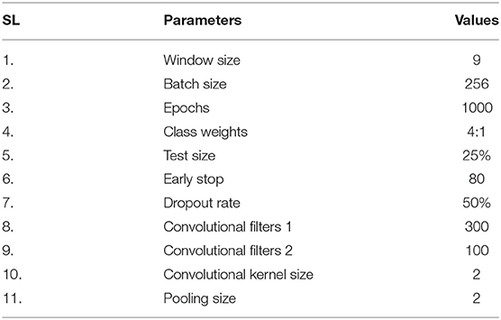
Table 3. Parameters used in CNN.

TABLE 4

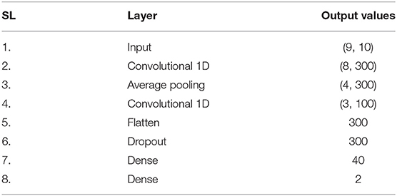
Table 4. CNN layers with their output size.

With maneuver-based features, the generated dataset is used to train several classifiers including the ANN, RF, k-NN, and SVM. The Python Deep Learning library Keras² is used for the implementation of ANN with using two fully connected layers with 128 neurons in each layer and a dropout=0.05. While the other ML algorithm is applied using scikit-learn library⁴ in Python. Here, a hyperparameters optimization is performed using a grid search to tune different classifier parameters. For the k-NN classifier (k=1), while the RF (n_estimators=41, min_samples_leaf=2, bootstrap=False, max_features=sqrt), the SVM (kernel=rbf, class_weight=balanced) as define in (Altarabichi et al., 2019).

Experimental Works

The main objective of this experimental work is to observe several ML algorithms and their classification accuracy as a performance. Here, the roundabout classification is considered where 10-folds cross validation (CV) is applied.

Considering Window-Based Features

The feature sets identified using window-based approach are used in 10-folds cross validation, where ML algorithms, CNN, HMM, RF and SVM are used. An average value for precision, recall and F₁-score are calculated considering both the roundabout and not/others classes and the results are presented in Table 5.

TABLE 5

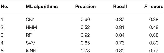
Table 5. Average classification results on both roundabout and not/others classes using several ML algorithms.

As can be observed form Table 5, the CNN and RF both achieved the highest F₁-score which is 88%, where highest precision is observed for RF, i.e., 92% and highest recall is observed by CNN, i.e., 87%. In CNN, the model achieved best training accuracy with improvements by trained the model for first 30 epochs whereas the validation-loss reached the lowest point in epoch 47. The comparison between the implemented ML algorithms considering F₁-score is presented in Figure 3, where both CNN and RF shows the highest score compare to other methods.

FIGURE 3

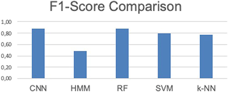
Figure 3. Comparison between the ML algorithms.

The confusion matrixes both for the CNN and RF are presented in Table 6. Here, we consider the topmost F₁-scores achieved by the ML algorithms i.e., CNN and RF.

TABLE 6

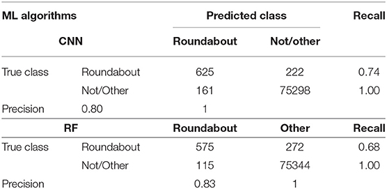
Table 6. Confusion matrixes for CNN and RF.

As can be observed from Table 6, the highest precision achieved for roundabout is 83% by RF and highest recall achieved for the roundabout is 74% by CNN. A Matthews Correlation Coefficient (MCC) is also calculated for CNN and RF to compare the algorithm defined in terms of True Positive (TP), True Negative (TN), False Positive (FP) and False Negative (FN) and the formula can be express as follows in eq2 (Boughorbel et al., 2017), the MCC results are presented in Table 7.

$\begin{array}{l}MCC=\frac{TP*TN-FP*FN}{\sqrt{(TP+FP)*(TP+FN)*(TN+FP)*(TN+FN)}}\end{array}$

TABLE 7

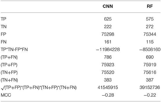
Table 7. MCC value on both roundabout and not/others classes using CNN and RF algorithms.

Considering Maneuver-Based Features

The ML approaches are again tested with maneuver-based features, that is the created models are validated using 10-folds cross validation. Here, instead of CNN, ANN is applied to compare with the rest of the ML algorithms, i.e., SVM, RF, and k-NN. An average value for precision, recall and F₁-score are calculated considering both the roundabout and not/others classes and the results are presented in Table 8.

TABLE 8

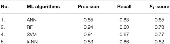
Table 8. Average classification results on both roundabout and not/others classes using several ML algorithms.

As can be seen from the table, ANN algorithm achieved the highest F₁-score on an average of roundabout and not/others classes i.e., 81% with similar precision and recall, i.e., 81% ≅ 82%. While, the k-NN algorithm achieved 2nd highest F₁-score which is 80% with 82% precision and 79% recall. The comparison between the implemented ML algorithms considering F₁-score presented in Figure 4, where both ANN shows the highest score compare to other methods and 2nd highest score was by k-NN.

FIGURE 4

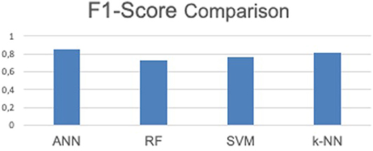
Figure 4. Comparison between the ML algorithms.

The confusion matrixes both for the ANN and k-NN are presented in Table 9. Here, we consider the topmost F₁-scores achieved by the ML algorithms i.e., ANN and k-NN.

TABLE 9

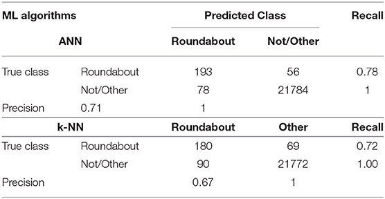
Table 9. Confusion matrixes for ANN and k-NN.

As can be observed from Table 9, both the highest precision and recall are i.e., 71 and 78%. achieved for the roundabout using the ANN algorithm. Similar to the Window-based Features, MCC is calculated and presented in Table 10.

TABLE 10

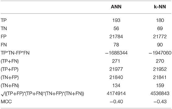
Table 10. MCC value on both roundabout and not/others classes using ANN and k-NN algorithms.

Comparison Between the Features

A comparison between the windows-based features and the maneuver-based features with their classification results are presented in Figure 5. Here, maximum F₁-Score and Maximum MCC value is considered out of several machine learning algorithms as presented earlier. As can be seen form the figure, both considering F₁-Score and MCC the windows-based features achieved the heights score in classification.

FIGURE 5

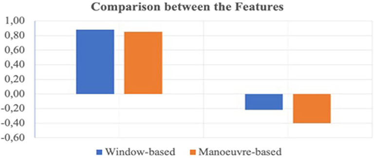
Figure 5. Comparison between the extracted features with Maximum F₁-Score and MCC.

Summary and Discussion

To achieve the goal of the project that is to create a realistic behavioral model the Naturalistic Driving Studies (NDS) has been performed to examine a real traffic situation by observing the drivers driving maneuver like roundabout. A total 16 volunteers are selected randomly and participated between May and August 2018. However, in window-based, labeled data set contains 76306 instances, of which 847 are labeled as roundabouts, and in maneuver-based it was 22111 instances with 249 roundabouts. As the study focuses on the roundabout identification not any individual's performance, thus the total sample size out of these 16 volunteers are enough for investigate several ML algorithms. To reduce the impractical task of identifying the maneuver manually by a human, this paper proposed a CNN to identify driving maneuver. Here, the collected IMU sensory data sets are used for the feature extraction, and both window-based and maneuver-based features are considered. And the GPS sensory data is used to label the data sets as the roundabout and not/others classes. Several ML algorithms including the CNN is investigated, and the other algorithms are: HMM, RF, ANN, k-NN, and SVM. A 10-fold cross validation is conducted and precision, recall and F₁-Score are calculated both for the roundabout and not/others classes and using window-based and maneuver-based feature sets. According to the results, CNN and RF achieved the best average F₁-Score i.e., 88% as an overall classification accuracy. However, while considering MCC, it shows RF shows the best correlation, i.e., −0.22, the reason of the imbalanced samples may affect the results where the study is about Very high TN to very low TP.

CNN methods seem to be the best option for the classification; however, it requires huge amount of data, thus using window-based features 76306 instances are used for generating the model. This also valid for ANN where only two connected hidden layers is used with 22111 instances. A manual inspection is also conducted on one driver data set, that is by plotting GPS data to observe the accuracy by the CNN model. It was observed that the CNN model classified nearly all roundabouts and major false positives false negatives are occurred because of they are either at start or end of the roundabout. The model also classifies some of the S-shaped road curves as roundabouts as observed. It was also found that there are some instances those can be said as “rare instance” of false positive, here, the geometry of the road is similar to a roundabout, e.g., entrance and exit to the highway. Again, some of the roundabout are so small that the driver just drives their car straight without any turning or a standard right turn are also identified as false negative. While labeling the data set, poor GPS data are also affected and make hard for manual task of labeling all the roundabout without any error. More narrow experiments could be conducted to explore the miss-classification at the starting point and the exit of roundabouts.

As a conclusion CNN could be used as a suitable method to classify roundabout, and RF could be the next suitable choice as it has higher precision than CNN. Also, the 88% F₁-Score shows satisfactory performance with an unbalance data set, but, the MCC value recommend to use RF. However, the observation shows better performance while using the window-based feature set extracted through CNN than the manuover-based features extracted in a sequence entrance -> in the roundabout -> exit.

CNN is considered to be the best classifier as the Recall of the algorithm is 87% i.e., the sensitivity of the roundabout is the fraction of the total amount of relevant instances that were actually retrieved. As the number of the roundabout classes are very less compare to other classes it may increase with CNN if the number of the sample increased and the dataset become balanced. Again, in maneuver-based features extraction ANN outperforms with 88% recall whereas RF was only 60%. Note, that ANN is a part of CNN with less network layer can used while there are not enough data samples. Also, However, none of other ML algorithms such as HMM, SVM, k-NN and ANN are unable to achieve satisfactory performance while identifying the driving manuover. Again, as the data set is collected through a Naturalistic Driving Studies (NDS) under a project called SimuSafe, around 20% data were affected due to sensor changes its positions. That is either or both the IMU and the GPS sensors are not faulty but while using it on the car the position of the sensor was change which was not notice until the data collection period is over. Thus, several of the instances are found with irregularities in either IMU or GPS or both as the mounted sensors are misplaced, which should be validate in future study with providing information to the user to correctly mounted sensors. More control and simulated studies are ongoing, e.g., in cycle 2, the test will be conducted in simulator environment and also in the truck. Thus, the data set can be more uniformly labeled and finally, a more balanced data set can be achieved. Then the study could be replicated using the more extensive data sets with the more uniform positioning of the IMU-sensor in the vehicle to minimize discrepancies. Three models i.e., CNN, RF, and ANN are implemented into a car's CAN for real manuover identification both in practical life-data collection and in simulators. Again, these will be tested in cycle 2 in SimuSafe, which is now suspended due to Corona predicament. SimuSafe aims to have bigger study using 400+ participants throughout of Europe (Sweden, Spain, Italy, France and UK) considering both controlled and simulated environment which is ongoing.

Data Availability Statement

The datasets presented in this article are not readily available because data sets are not open and published yet by the Project. Requests to access the datasets should be directed to Marteyn van Gasteren, marteyn.vangasteren@itcl.es.

Author Contributions

MA initiate the paper, he wrote the most of the chapter of the manuscripts excepts introduction and discussion. SB wrote the introduction and discussion of the paper and also reviewed the whole manuscript. All authors contributed to the article and approved the submitted version.

Funding

SimuSafe, the project has received funding from the European Union's Horizon 2020 research and innovation programme under grant agreement no. 723386.

Conflict of Interest

The authors declare that the research was conducted in the absence of any commercial or financial relationships that could be construed as a potential conflict of interest.

Acknowledgments

Authors want to acknowledge all the participants who were involved in this study, to give permission to mount IMU and GPS sensors on their cars and they have used their cars for several weeks regularly. Also, many thanks to our students Adrian Fager, Emil Lundin, Patrik Forsslund, Anton Roslund, and Jakob Norin to perform the initial implementation with close supervision by the project members.

Footnotes

1. ^http://simusafe.eu/

2. ^https://keras.io/

3. ^http://users.cecs.anu.edu.au/~Peter.Christen/Febrl/febrl-0.3/febrldoc-0.3/node25.html

4. ^https://scikit-learn.org/stable/

References

Ahmed, M. U., Begum, S., Catalina, C. A., Limonad, L., Hök, B., and Flumeri, G. D. (2017). “Cloud-based Data Analytics on Human Factor Measurement to Improve Safer Transport (Nov 2017),” in 4th EAI International Conference on IoT Technologies for HealthCare (HealthyIoT'17), (Angers). doi: 10.1007/978-3-319-76213-5_14

CrossRef Full Text | Google Scholar

Al-luhaibi, S. K., Said, A. M., and Najim Al-Din, M. S. (2018). Recognition of Driving manoeuvre Based Accelerometer Sensor. Int. J. Civil Eng. Technol. 9, 1542–1547. Available online at: http://www.iaeme.com/MasterAdmin/Journal_uploads/ijciet/VOLUME_9_ISSUE_11/IJCIET_09_11_149.pdf

Google Scholar

Altarabichi, M. G., Ahmed, M. U., and Begum, S. (2019). “Supervised learning for road junctions identification using IMU (Mar),” in First International Conference on Advances in Signal Processing and Artificial Intelligence (ASPAI' 2019).

Google Scholar

Attal, F., Boubezoul, A., Oukhellou, L., and Espié, S. (2013). “Riding patterns recognition for Powered two-wheelers users' behaviors analysis,” in IEEE Conference on Intelligent Transportation Systems, Proceedings, ITSC, (The Hague). doi: 10.1109/ITSC.2013.6728528

CrossRef Full Text | Google Scholar

Barnard, Y., Utesch, F., van Nes, N., Eenink, R., and Baumann, M. (2016). The study design of UDRIVE: the naturalistic driving study across Europe for cars, trucks and scooters. Eur. Transp. Res. Rev. 8:14. doi: 10.1007/s12544-016-0202-z

CrossRef Full Text | Google Scholar

Basheer, I. A., and Hajmeer, M. (2000). Artificial neural networks: fundamentals, computing, design, and application. J. Microbiol. Methods 43, 3–31. doi: 10.1016/S0167-7012(00)00201-3

PubMed Abstract | CrossRef Full Text | Google Scholar

Boughorbel, S., Jarray, F., and El-Anbari, M. (2017). Optimal classifier for imbalanced data using Matthews Correlation Coefficient metric. PLoS ONE 12:e0177678. doi: 10.1371/journal.pone.0177678

PubMed Abstract | CrossRef Full Text | Google Scholar

Breiman, L. (1996). Bagging predictors. Mach. Learn. 24, 123–140. doi: 10.1023/A:1018054314350

CrossRef Full Text | Google Scholar

Breiman, L. (2001). Random forests. Mach. Learn. 45, 5–32. doi: 10.1023/A:1010933404324

CrossRef Full Text | Google Scholar

Di Lecce, V., and Calabrese, M. (2009). “NN-based measurements for driving pattern classification,” in 2009 IEEE Instrumentation and Measurement Technology Conference (Singapore), 259–264. doi: 10.1109/IMTC.2009.5168455

CrossRef Full Text | Google Scholar

Drew, P. J., and Monson, J. R. T. (2000). Artificial neural networks. Surgery 127, 3–11. doi: 10.1067/msy.2000.102173

PubMed Abstract | CrossRef Full Text | Google Scholar

Ertel, W. (2018). Introduction to Artificial Intelligence. Springer, 658–652. Available online at: https://www.springer.com/gp/book/9783319584867

Google Scholar

Fagnant, D. J., and Kockelman, K. M. (2013). Preparing a Nation for Autonomous Vehicles: Opportunities, Barriers and Policy Recommendations. Eno Foundation. Available online at: https://www.caee.utexas.edu/prof/kockelman/public_html/ENOReport_BCAofAVs.pdf (accessed July 06, 2020).

Google Scholar

Feng, G. (2019). Statistical Methods for Naturalistic Driving Studies. Ann. Rev. Stat. Appl. 6, 309–328. doi: 10.1146/annurev-statistics-030718-105153

CrossRef Full Text | Google Scholar

Fernandes de Mello, R., and Antonelli Ponti, M. (2018). A Brief Review on Machine Learning. Cham: Springer International Publishing, 1–74. doi: 10.1007/978-3-319-94989-5_1

CrossRef Full Text | Google Scholar

Friedman, J., Hastie, T., and Tibshirani, R. (2001). The Elements of Statistical Learning. New York, NY: Springer Series in Statistics.

Google Scholar

Gerdes, A. (2006). “Automatic manoeuvre recognition in the automobile: the fusion of uncertain sensor values using bayesian models,” in Proceedings of the 3rd International Workshop on Intelligent Transportation (WIT 2006) (Hamburg), 129–133.

Google Scholar

Gonzalez, D., Prez, J., and Milans, V. (2017). Parametric-based path generation for automated vehicles at roundabouts. Exp. Syst. Appl. 71, 332–341. doi: 10.1016/j.eswa.2016.11.023

CrossRef Full Text | Google Scholar

Guyon, I., Weston, J., Barnhill, S., and Vapnik, V. (2002). Gene selection for cancer classification using support vector machines. Mach. Learn. 46, 389–422. doi: 10.1023/A:1012487302797

CrossRef Full Text | Google Scholar

Hernández Sánchez, S., Fernández Pozo, R., and Hernández Gómez, L. A. (2018). Estimating vehicle movement direction from smartphone accelerometers using deep neural networks. Sensors (Basel) 18:2624. doi: 10.3390/s18082624

PubMed Abstract | CrossRef Full Text | Google Scholar

Ho, T. K. (1995). “Random decision forests,” in Proceedings of 3rd International Conference on Document Analysis and Recognition (Montreal, QC), 278–282.

Google Scholar

Johnson, D. A., and Trivedi, M. M. (2011). “Driving style recognition using a smartphone as a sensor platform,” in 2011 14th International IEEE Conference on Intelligent Transportation Systems (ITSC) (Washington, DC), 1609–1615. doi: 10.1109/ITSC.2011.6083078

CrossRef Full Text | Google Scholar

KPMG (2012). Self-Driving Cars: The Next Revolution. KPMG and the Center for Automotive Research. Available online at: http://www.cargroup.org/wp-content/uploads/2017/02/Self_driving-cars-The-next-revolution.pdf (accesed July 06, 2020).

Google Scholar

Larose, D. T. (2005). Discovering Knowledge in Data: An Introduction to Data Mining. John Wiley and Sons, Inc. doi: 10.1002/0471687545.ch5

CrossRef Full Text | Google Scholar

Li, S. Z., and Jain, A. (Eds.) (2009). Baum-Welch Algorithm. Boston, MA: Springer US. doi: 10.1007/978-0-387-73003-5_539

CrossRef Full Text | Google Scholar

Ma, Y., Zhang, Z., Chen, S., Yu, Y., and Tang, K. (2019). A comparative study of aggressive driving behavior recognition algorithms based on vehicle motion data. IEEE Access 7, 8028–8038. doi: 10.1109/ACCESS.2018.2889751

CrossRef Full Text | Google Scholar

Muronga, K. (2017). The Effectiveness of the Naturalistic Driving Studies in Improving Driver Behavior, Submitted as a Mini-Dissertation and Partial Requirement for The Degree: Magister Technologiae: Business Information Systems. Pretoria: Tshwane University of Technology.

Google Scholar

Ouyang, Z., Niu, J., and Guizani, M. (2018). Improved vehicle steering pattern recognition by using selected sensor data. IEEE Trans. Mobile Comput. 17, 1383–1396. doi: 10.1109/TMC.2017.2762679

CrossRef Full Text | Google Scholar

Pilko, H., Bri, D., and Ubi, N. (2014). Study of vehicle speed in the design of roundabouts. Graevinar 66, 407–416. doi: 10.14256/JCE.887.2013

CrossRef Full Text | Google Scholar

Rabiner, L. R. (1989). A tutorial on hidden markov models and selected applications in speech recognition. Proc. IEEE 77, 257–286. doi: 10.1109/5.18626

CrossRef Full Text | Google Scholar

Robert, C. (2014). Machine learning, a probabilistic perspective. CHANCE, 27, 62–63. doi: 10.1080/09332480.2014.914768

CrossRef Full Text | Google Scholar

Van Ly, M., Martin, S., and Trivedi, M. M. (2013). “Driver classification and driving style recognition using inertial sensors,” in 2013 IEEE Intelligent Vehicles Symposium (IV) (City of Gold Coast), 1040–1045. doi: 10.1109/IVS.2013.6629603

CrossRef Full Text | Google Scholar

Vapnik, V. N. (1992). Principles of Risk Minimization for Learning Theory. Adv. Neural Information Process. Syst. 4, 831–838.

Google Scholar

Waga, K., Tabarcea, A., Chen, M., and Fränti, P. (2012). “Detecting movement type by route segmentation and classification,” in 8th International Conference on Collaborative Computing: Networking, Applications and Worksharing (Pittsburgh, PA: CollaborateCom), 508–513. doi: 10.4108/icst.collaboratecom.2012.250450

CrossRef Full Text | Google Scholar

Yiyan, L., Fang, Z., Wenhua, S., and Haiyong, L. (2017). “An hidden Markov model based complex walking pattern recognition algorithm,” in 4th International Conference on Ubiquitous Positioning, Indoor Navigation and Location-Based Services – Proceedings of IEEE UPINLBS (Shanghai), 223–229.

Google Scholar

Zardosht, M., Beauchemin, S. S., and Bauer, M. A. (2018). Identifying driver behavior in preturning manoeuvre using in-vehicle CANbus signals. J. Adv. Transport. 2018:5020648. doi: 10.1155/2018/5020648

CrossRef Full Text | Google Scholar

Zhang, G. P. (2000). Neural networks for classification: a survey. Syst. Man Cybernet. Part C 30, 451–462. doi: 10.1109/5326.897072

CrossRef Full Text | Google Scholar

Zhao, M., Kathner, D., Jipp, M., Soffker, D., and Lemmer, K. (2017). “Modeling driver behaviour at roundabouts: results from a field study,” in 2017 IEEE Intelligent Vehicles Symposium (IV) (Redondo Beach, CA), 908–913. doi: 10.1109/IVS.2017.7995831

CrossRef Full Text | Google Scholar

Zheng, Y., and Hansen, J. H. L. (2016). “Unsupervised driving performance assessment using free-positioned smartphones in vehicles,” in 2016 IEEE 19th International Conference on Intelligent Transportation Systems (ITSC), (Rio de Janeiro), 1598–1603. doi: 10.1109/ITSC.2016.7795771

CrossRef Full Text | Google Scholar