EquiSim: An Open-Source Articulatable Statistical Model of the Equine Distal Limb

1. Introduction

Digital three-dimensional (3D) anatomical models have become an important aspect in the digitalization of veterinary research and medical practices (1). Being acquired by computed tomography (CT) imaging or magnetic resonance imaging (MRI) (2) or by 3D optical scanning (3), those subject-specific models find their way into finite element analyses (FEA) (4), augmented reality guidance during operations (5), and training of radiograph segmentation networks (6).

A standard procedure in morphological studies of equine distal limb anatomical structures focuses on one-dimensional linear or angular measures, such as hoof angle, hoof length, medial-lateral width of the phalanges, and so on, or two-dimensional measures, such as the joint surface. They are measured from radiographs (7, 8), MRI data (9), photographs (8, 9), or from in-situ measurements in vivo (10, 11) or post-mortem (12).

Another way to study morphology variations is by means of statistical shape models (SSMs), which encode the 3D shape variation of the complete bone geometry, rather than reducing the shape to a limited set of discrete measures (13). The benefit of this representation, compared to linear biometrics, is that the statistical shape variability is defined as variation modes of the geometry itself, such that it can be exploited in numerous computer vision applications. In human medical research, these (articulating) SSMs have been widely adopted for training segmentation neural networks on CT data (14, 15). The models also provide prior shape information for the reconstruction of personalized 3D models from sparse point-data (16) or from two-dimensional radiographs (17, 18), to facilitate orthopaedic computer-assisted surgeries (CAS), or to generate personalized finite element models for mechanical simulations (19, 20). Integrated in deep learning techniques, the models can discriminate between pathological cases based on morphing parameters and thereby outperforms manual subjective classification (21). The inherent geometric information can also be used to study the relationship between shape and biomechanical functions (22).

Because of additive manufacturing or 3D printing, physical models can efficiently be (re-)produced from these digital models (23). Rapid prototyping has been deployed as didactic material in anatomy classes to study anatomy besides classical dissection sessions and for training of surgery techniques as an alternative to experimental animals (24, 25). Orthopedic implant design also benefits from computer-aided design (CAD) and 3D printing, as their design can be customized (26, 27). Osteosynthesis plates can be designed specifically according to the individual anatomy prior to fabrication of the plates. CAD thereby omits inter-operative bending of the plates as is the case with off-the-shelf template designs. It has been claimed that customized implant designs, which take the shape variability into account, improve the clinical outcome (27).

Despite the many potential applications, SSMs remain underexplored in veterinary research. First, this is due to lack of availability of large collections of 3D data, from which such model can be built. Most available models are static and subject specific and are therefore less relevant for CAD. Second, there is no one-to-one relation between the variation modes of an SSM and the linear biometrics. This might complicate the interpretation of SSMs and make them less attractive for veterinarians.

In the field of equine veterinary research, we see most potential applications for SSMs to the equine distal limb. The shape of the horse's distal limb bones is an important factor in determining the horse's performance. Because the phalanges and metacarpal bones distribute the impact forces upon landing on the ground, the shape (and bone mineral density) of the bones affect how efficiently forces are distributed and subsequently determine its risk of fractures (28). It has also been observed that hoof conformation is correlated to movement asymmetry (29). Uneven foot-bearing can eventually lead to biomechanical injuries or lameness, and should be taken into account for corrective shoeing and farriery (30, 31).

The aim of this paper is to provide a workflow to generate an articulating SSM of the equine distal limb. Furthermore, the SSM's variation modes are associated with conventional linear biometrics in order to ease the model interpretation. Unlike earlier SSMs, our model describes the statistical shape variation of the different bones simultaneously in one model. This ensures correct jointspace distances for different model instances and enables articulation of the model toward different poses.

We first outline the methodology to construct an articulating multi-component statistical shape model (aSSM) of the equine distal limb, which is based on the earlier work of (17). Next, we describe the major statistical variation modes in terms of linear biometrics. In the discussion, we provide directions of future research and potential application areas in the field of veterinary research where the model can be adopted.

2. Materials and Methods

2.1. Data Collection and Data Preparation

A random collection of 70 left and right distal front limbs of 35 cold-blooded and warm-blooded horses and ponies was donated by a commercial abattoir and bulk CT-scanned post-mortem with a Canon Aquilion LB CT system (resolution: (0.78×0.78×0.5) mm³, tube current: 200 mA, generator power: 27 kW) from the hoof to the carpus. All legs were unshod at the time of scanning. The hoofs did not undergo prior hoof trimming or cleaning. Right limbs were later mirrored to resemble left limbs.

The acquired CT images were segmented using an open-source graph-cut multi-label segmentation technique (32), followed by minor manual corrections. The segmentation label maps were converted to digital geometry surface models by a discrete marching cube algorithm (33) and re-meshed to a coarser curvature-adaptive mesh by ACVD-software (34). Mesh artifacts were eventually resolved by MeshFix (35).

2.2. Construction of the Articulating Multi-Component Statistical Shape Model

In this section, we describe the proposed methodology to build a compact representation model of the shape variations in our population of L = 70 equine distal limb models S_i, i ∈ {0, …, L}, with i = 0 indicating the reference model that was adopted from earlier work (6). As illustrated in Figure 1A, each limb model S_i consists of M = 10 components (nine distal limb bones and the hoof capsule); thus, S_i = {S_ij, j = 0, …, M − 1}, where S_ij is the jth component of the ith subject with N_ij vertices. We denote the homogeneous vertex coordinates of shape S_ij by $v_{ij}=\left\{v_{ijp}\in {\text{ℝ}}^4,p=0,\dots ,N_{ij}-1\right\}$. The number of vertices per component j of the reference model are tabulated in Table 1 and the resolution of the reference model is visualized in Figure 1B.

FIGURE 1

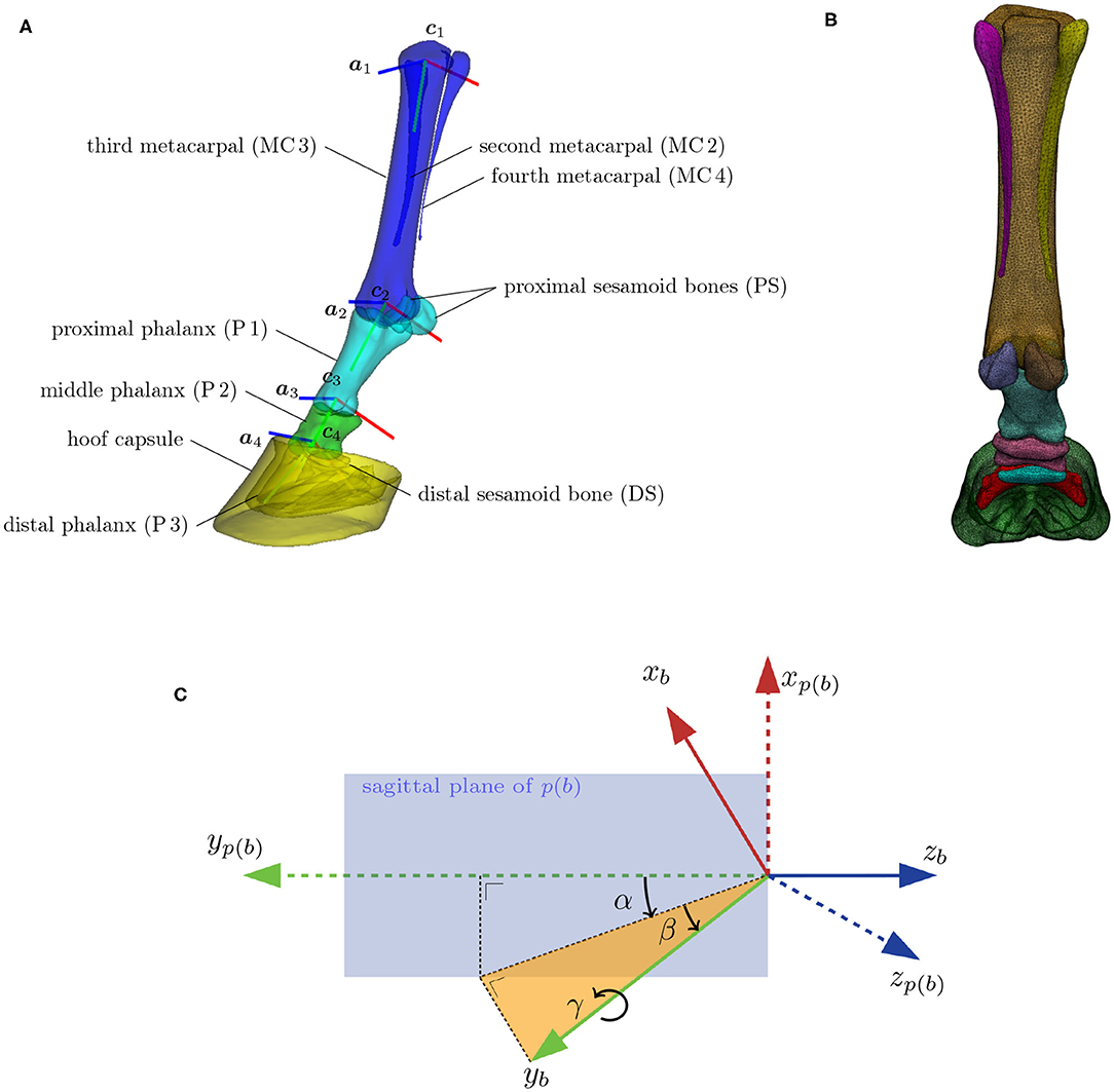
Figure 1. (A) The distal limb model consisting of nine bones and the hoof capsule. Bones with similar colors move rigidly under skeleton articulation. Each bone has a local orthogonal reference frame (x_b, y_b, z_b) associated with it, which are here represented by, respectively, the red, green, and blue lines. The flexion/extension rotation axis of bone b is denoted by a_b and is positioned at location c_b. The flexion/extension around axes a₂, a₃, and a₄ are the major degrees of freedom of the articulation model. (B) Model with overlayed wireframe, indicating the resolution of the surface model. (C) Definition of the spherical angles (α, β, γ) between a bone's reference frame (x_b, y_b, z_b), and its adjacent parent bone's reference frame [x_p(b), y_p(b), z_p(b)]. The extension/flexion angle α between two adjacent bones is measured inside the sagittal plane of the parent bone. The corresponding rotation axis a_b coincides with the z-axis of the parent bone z_p(b). The abduction/adduction angle β is measured perpendicular to the sagittal plane of the parent bone. The associated rotation axis is y_b × z_p(b). The internal rotation γ happens around the bone axis y_b itself.

TABLE 1

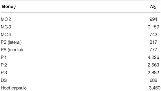
Table 1. Number of vertices per component of the reference model.

2.2.1. Articulation Model

Articulation of the surface model, as illustrated in Figure 2 for the different stages of the stance phase, is limited to the major degrees of freedom of the equine distal limb. This includes the extension and flexion around the following three joints: metacarpophalangeal (MCP), proximal interphalangeal (PIP), and the distal interphalangeal (DIP). The articulation model articulates the proximal sesamoid bones and the proximal phalanx as one geometry structure (38). This approximation is justified by their relatively small range of motion and any latent motion, which happens in reality, will end up as a shape variability in the model. Similarly, the distal sesamoid bone and the hoof capsule are assumed to be rigidly attached to the distal phalanx in the articulation model. Furthermore, the three metacarpal bones are rigidly attached to each other. Under these assumptions, the articulation model effectively consists of N_b = 4 skeleton bones to transform M = 10 surface model components.

FIGURE 2

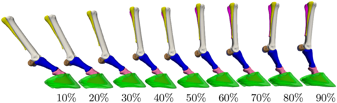
Figure 2. Distal limb model's articulation throughout the stance phase. The percentages indicate the completion level of the stance phase. Extension/flexion angles for the metacarpophalangeal (MCP), proximal interphalangeal (PIP), and distal interphalangeal (DIP) joints were obtained from the literature (36, 37).

The articulation model assigns a local reference frame to each of the four skeleton bones, as depicted in Figure 1A. The orthogonal reference frame is defined such that its y-axis aligns with the elongation axis and that its z-axis is perpendicular to the sagittal plane of the bone. The flexion, abduction and internal rotation angle are, respectively, identified as the three spherical coordinates (α, β, γ) between adjacent reference frames. Their definition is visualized in Figure 1C. Note that the flexion rotation axis a of bone b corresponds to the z-axis of its parent bone p(b).

To enable articulation of the distal limb bones themselves, we also define an origin c to each reference frame, which is chosen as the center of a circle, fitted to the joint surface area of the bone in its sagittal plane. The local-to-world transformation T ∈ ℝ^4×4 brings the local reference frame of a bone, like the one shown in Figure 1C, to its position and orientation in world coordinates. Flexion of a bone b relative to its parent bone p(b) over an angle θ is obtained by the transformation $T_{p(b)}{R}_z(\theta )T_{p(b)}^{-1}$, where $R_z(\theta )\in {\text{ℝ}}^{4\text{×}4}$ represents a rotation over the z-axis. It should be noted that the articulation model is a mathematical construction and is not statistically founded by dynamic data.

2.2.2. Elastic Registration

Initially, each subject S_i in the training database is described by its own set of vertices. To statistically describe the shape variations in this database, all shapes must be in semantic correspondence with each other, such that vertices with the same index have the same anatomical location on all training subjects. In order to do so, we elastically deform the reference component coordinates $T_{ij}{T}_{0j}^{-1}{v}_{0j}$ toward its corresponding training subject component S_ij and replace the training subject by the registration result, without change of notation, such that each training shape is now described by the same semantic-meaningful mesh (39).

In order to reduce a possible bias toward the chosen reference model, we repeat the elastic registration with the mean model as reference. Note that registered shapes are still in their original position and orientation. Replacing the subject by its registered result introduces a geometric error of how well the original surface is approximated by its registered surface. As illustrated in Figure 3, this geometric error is highly position dependent, but overall negligible. The average unsigned geometric error over the entire model equals 0.182 ± 0.002 mm.

FIGURE 3

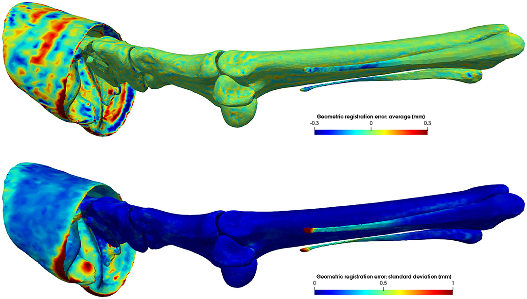
Figure 3. Average signed geometric error of the elastic surface registration to L = 70 subjects. Vertices of the registered reference model that lie inside or outside the target model have a negative or positive distance, respectively. The average error is a measure of the registration accuracy, while its variance is a measure of the precision of the registration.

2.2.3. Scale and Pose Normalization

As we are interested in the intrinsic shape variability, we want to normalize all training subjects for their global scale. All models were scale normalized based on the length of the third metacarpal of the reference model.

Second, training subjects were originally scanned on their side in different unloaded poses, which causes unwanted pose variations in the dataset. The pose normalization of bone b involves finding the optimal flexion angle θ^*, in a least-square sense, which matches the bone's geometry with the corresponding bone of the reference model in the local reference frame of its parent bone p(b):

$\begin{array}{ll}{\theta }^{*}=arg{\displaystyle \underset{\theta }{min}}\parallel T_{0j}^{-1}{v}_{0j}-R_z(\theta )T_{ij}^{-1}{v}_{ij}{\parallel }^2,& (1)\end{array}$

where the one-to-one correspondences from the previous step are exploited for the geometry matching. Note that we only optimize for the extension/flexion angle and not for abduction, adduction, and internal rotation, which are considered as remnant posture in the shape analysis.

2.2.4. PCA-Based Statistical Shape Modeling

Assuming a database of L registered pose- and scale-normalized shapes S_i, we can define each shape by its shape vector $s_i\in {\text{ℝ}}^{3F}$, which is a concatenation of its $F=\sum _{j=0}^{M-1}{N}_{0j}$ coordinates. The shape vectors of the L subjects are ordered as columns in a data-matrix X ∈ ℝ^3F×L.

The goal of principal component analysis (PCA) is to find an orthogonal transformation that transforms the high-dimensional shape vectors to a low-dimensional set of linearly uncorrelated variables, which are called principal components (PCs) (13). The PCs can efficiently be calculated by first mean-centering the rows of X and next performing a singular value decomposition (SVD) on the low-dimensional matrix X^TX. The matrix X multiplied by the left singular vectors of this decomposition are equal to the principal component vectors $u_i\in {\text{ℝ}}^{3F}$ of X, after normalizing the columns. The singular values of the decomposition are equal to the variances ${\sigma }_i^2$ of those PCs. The PCs are ordered such that the first PC accounts for the largest variation in the dataset, and each succeeding PC has the largest variance possible under the condition that it must be orthogonal to any previous component. Any shape can now be expressed as a linear combination of those PCs, weighted by its standard deviations:

$\begin{array}{ll}s(b)=\overline{s}+{\displaystyle \sum _{i=1}^{L-1}{b}_i}{\sigma }_i{u}_i& (2)\end{array}$

with $\overline{s}\in {\text{ℝ}}^{3F}$ the mean shape vector and b_i the contribution of the ith normalized PC u_i to the final shape s. In matrix notation, this reads:

$\begin{array}{ll}s(b)=\overline{s}+EDb& (3)\end{array}$

where the columns of matrix E ∈ ℝ^3F×L−1 contain the normalized eigenvectors u_i and $D=\mathrm{\text{diag}}({\sigma }_1,{\sigma }_2,\dots ,{\sigma }_{L-1})\in {\text{ℝ}}^{L-1\times L-1}$. The PC weights b ∈ ℝ^L−1 allow to generate new shape instances from the SSM, different from the training data. Given a new shape s with the same topology as the SSM, the PC weights that approximate this new shape most closely are given by:

$\begin{array}{ll}b=D^{-1}{E}^{+}(s-\overline{s}),& (4)\end{array}$

with E⁺ the pseudo-inverse of the non-square matrix E.

2.2.5. Articulating Statistical Shape Model Construction

Applying PCA to the set of registered pose- and scale-normalized shape coordinates ${ṽ}_{ij}=R_z({\theta }^{*})T_{ij}^{-1}{v}_{ij}$, it is important for each shape vector s_i to also contain skeleton information besides the geometry coordinates, because both are intertwined: if the shape changes, the underlying skeleton will have to be modified as well in order to maintain proper articulation. The shape vector is therefore a concatenation of the geometry coordinates of all components of the model and the position c_b and orientation a_b of the rotation axes of the bones in the skeleton model, as shown in Figure 1A:

$\begin{array}{l}{s}_i=[\underset{\text{geometry coordinates}}{\underbrace{{\tilde{v}}_{i,0}{\tilde{v}}_{i,1}\dots {\tilde{v}}_{i,M-1}}}\underset{\text{axis orientation}}{\underbrace{{\log }_{{\mu }_1}{a}_1^i{\log }_{{\mu }_2}{a}_2^i\dots {\log }_{{\mu }_{N_b}}{a}_{N_b}^i}}\\ \underset{\text{axis position}}{\underbrace{c_1^i{c}_2^i\dots c_{N_b}^i}}{]}^T\in \text{}{\text{ℝ}}^{3F},& (5)\end{array}$

with $F=\sum _{j=0}^{M-1}{N}_{0j}+2N_b$. Note that we take a logarithmic map of the axis orientation vectors a_b around their intrinsic means μ_b, because PCA assumes that the data are normally distributed in an Euclidean (high-dimensional) space. However, the rotation vectors are constrained to lie on the unit sphere S², meaning that their length is always one and they can only vary in their orientation. Hence, the vectors lie on a curved manifold and one needs to adopt principal geodesic analysis (PGA) instead of PCA to describe the data variability (40). In short, it applies PCA on the tangent space of S², and one needs to use the logarithmic and exponential map around the intrinsic mean to move back and forth between S² and the Euclidean tangent space.

The reconstruction of a component j from the articulating SSM is obtained via:

$\begin{array}{ll}s(b,{\theta }_j)=(T(b)◦R_z({\theta }_j))s(b),& (6)\end{array}$

where s(b) can be calculated from Equation (3). Note that the transformation T is also dependent on b as it depends on the rotation axis and center of the bones.

2.3. Biometrics

Biometrics are linear or angular measures that characterize a component's shape and can be expressed in terms of the variation modes of the SSM. We consider biometrics for the hoof capsule, the third phalanx (7–11), the third metacarpal, the first and second phalanx (12), and the distal sesamoid bone. The definitions of the selected biometrics are tabulated in Table 2. The metrics were automatically calculated on the 3D geometry models, instead of on two-dimensional images as is often done in the literature. Figure 4 shows the biometrics indicated on the 3D models.

TABLE 2

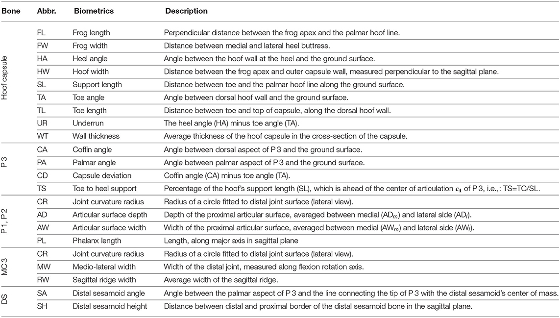
Table 2. Definition of the biometrics, indicated on the 3D models in Figure 4.

FIGURE 4

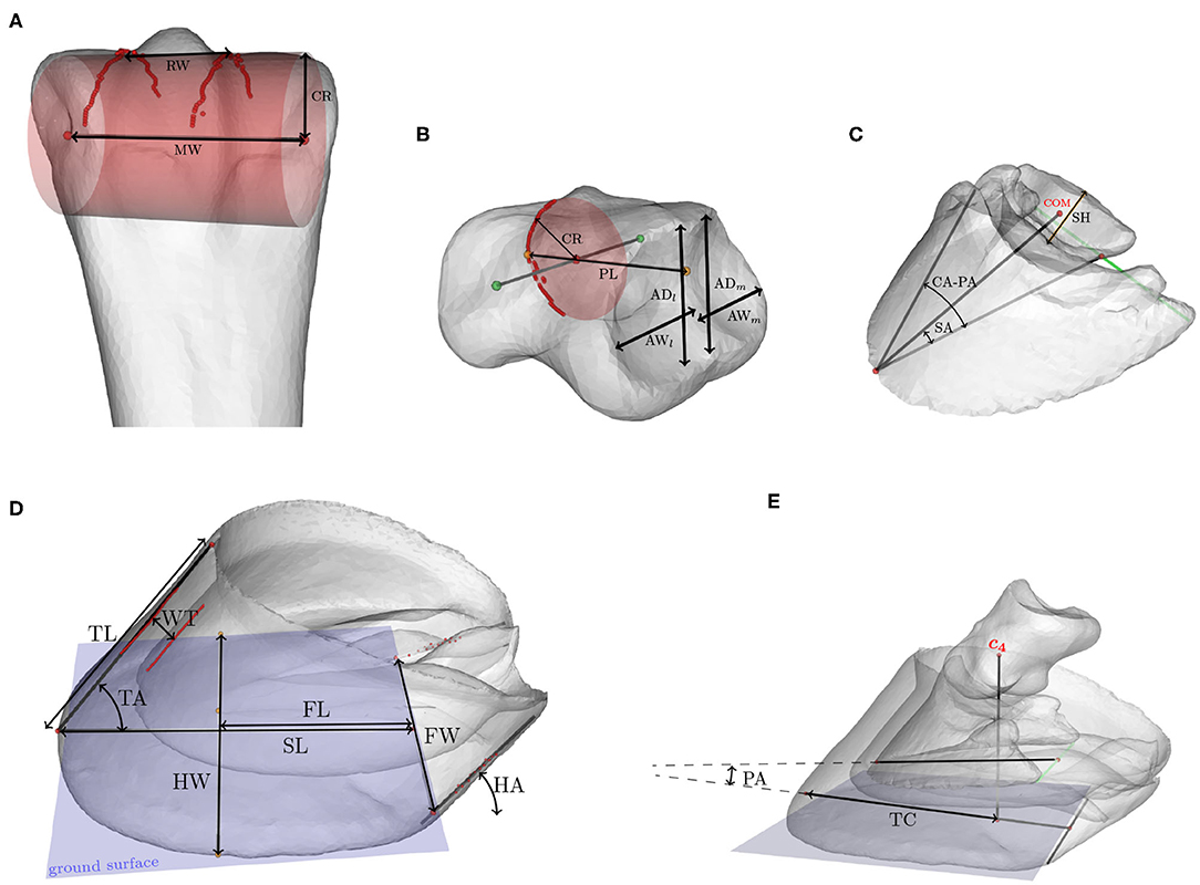
Figure 4. Biometrics indicated on the 3D models of (A) the third metacarpal, (B) the proximal or middle phalanx, (C) the distal phalanx and distal sesamoid bone, and (D) the hoof capsule. (E) shows the relative position of the distal and middle phalanx with respect to the hoof capsule. Abbreviations of the metrics are explained in Table 2.

2.3.1. Correlation Between Biometrics and PC Modes

In order to change the shape (i.e., changing the PC weights) as a function of the biometric, we applied a multivariate linear regression between the set of PC weights b and the biometric value k:

$\begin{array}{ll}b(k)=\left[\begin{array}{cc}\alpha & \beta \\ \end{array}\right]\left[\begin{array}{c}1\\ k\\ \end{array}\right].& (7)\end{array}$

The regression coefficients α, β ∈ ℝ^L−1 represent the offset and slope, respectively. They are determined from simulated model instances (N = 1, 000), created from the SSM by using Equation (6) following its multivariate normal distribution.

Given a biometric value, the linear regression estimates the PC weights, from which the corresponding SSM's instance can be reconstructed by Equation (6). Figure 5 shows a number of model instances corresponding to the biometric values μ − 3σ and μ + 3σ. Obviously, changing one biometric also changes other biometrics as they are all correlated with each other. In order to visualize the correlations between the different biometrics, we show the Pearson's correlation coefficients in Table 3.

FIGURE 5

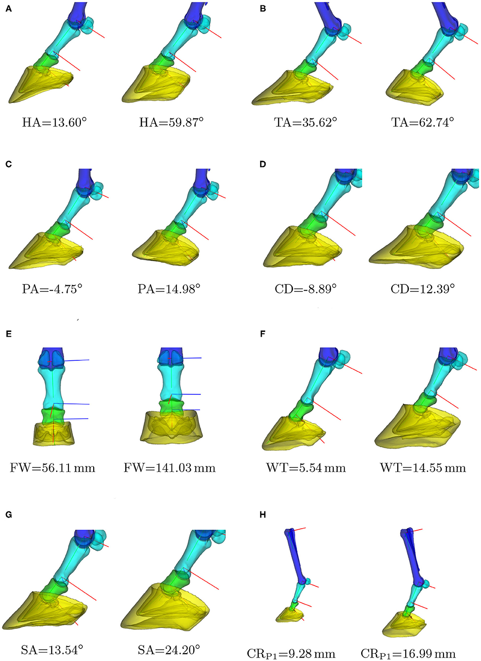
Figure 5. Instances of the statistical shape model (SSM) for different biometric values. For each biometric k, the models are shown that correspond to k = μ − 3σ and k = μ + 3σ, with μ and σ the average and standard deviation of the biometric in our dataset. Clipped models are shown to draw the reader's attention to the hoof area. In case of the curvature radius (H), one can notice the global scaling of the phalanges and hoof capsule with respect to the third metacarpal. (A) Heel angle, (B) toe angle, (C) palmar angle, (D) capsule deviation, (E) frog width, (F) hoof wall thickness, (G) distal sesamoid angle, (H) P1: joint curvature radius.

TABLE 3

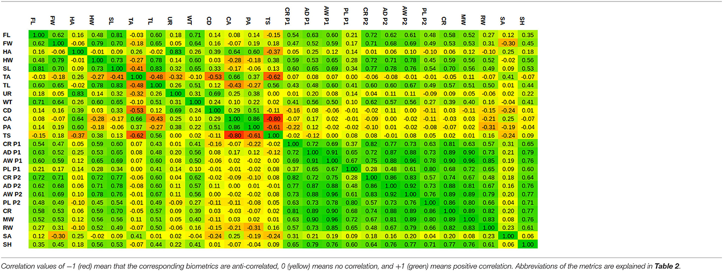
Table 3. Autocorrelation table of the biometrics.

3. Results

3.1. Model Performance

The statistical shape model's performance was evaluated in terms of compactness, generalizability, and specificity (41, 42) and are shown in Figure 6 as a function of number of PC modes. The compactness shows the cumulative variance explained by the statistical modes. Figure 6A indicates that the first 20 modes describe 95% of the variability in the training dataset. The model's specificity, shown in Figure 6B, is the extent to which the model can generate instances of the object that are close to those of the training set. To calculate this measure, random samples of the SSM have been generated by using Equation (6), according to its multivariate normal distribution. Each model instance has been compared to its closest training shape in the shape space, in terms of the root mean square error of the distance between corresponding vertices.

FIGURE 6

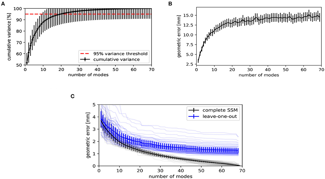
Figure 6. Evaluation metrics of the statistical shape model, as a function of number of principal component (PC) modes. (A) The compactness shows the cumulative variance explained by the statistical shape model (SSM). (B) The specificity indicates how similar randomly generated instances are to the training shapes. (C) Geometric error when fitting the SSM to unseen shapes (generalizability, blue) and to training shapes on which the SSM was built (reconstruction error, black). The faint lines show the geometric error per subject. The solid lines show the average of all subjects.

The generalizability indicates how well the model can be generalized to new subjects. A leave-one-out test has been performed for calculating this measure. The SSM has been rebuilt for L − 1 subjects and Equation (4) has been used to fit the obtained model to the subject being left out. Figure 6C shows the root mean square error between the subject being left out and the fitted result. We also show the reconstruction error when fitting to the same subject with the complete model, i.e., when the subject to which has been fitted is included in the training data. The discrepancy between both curves is the effect of fitting to unknown subjects. When using the model to fit to new instances, one might expect an average geometric error of 2.0 ± 0.3 mm when using the first 20 PC modes, as can be concluded from Figure 6C.

3.2. Biometrics

The generation of model instances based on a biometric value, as illustrated in Figure 5, exploits the multivariate regression relation given in section 2.3.1. The linear assumption of this regression has been evaluated by recalculating the biometric value $\tilde{k}$ on the model instance s(b(k), θ_j), created with the biometric value k. The absolute difference between the value k used to generate the model and the recomputed value $\tilde{k}$ on this model results in a confidence interval on k, which is reported in Table 4 and gives a measure for the nonlinearity of the relation between PC weights and the biometric.

TABLE 4

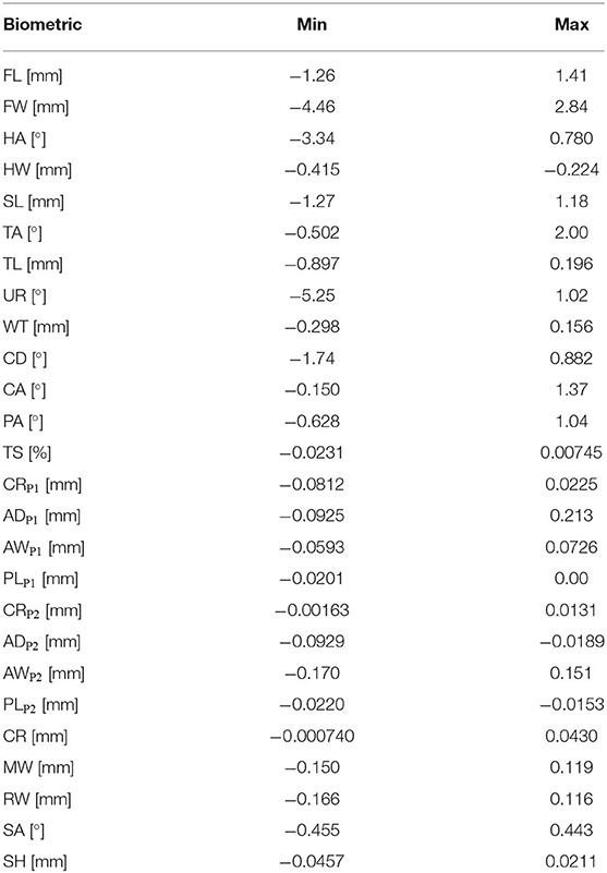
Table 4. Confidence intervals for the biometrics.

Nonlinear effects have dominantly been observed for the angle biometrics, especially for the heel angle and the under-run. Despite the nonlinearity, the accuracy of the other angular biometrics is less than two degrees for the full range of [μ − 3σ, μ + 3σ]. Most linear biometrics are sub-millimeter accurate. Only the frog width, frog length, capsule deviation, and the support length of the hoof capsule have a larger difference between the expected and measured biometric.

4. Discussion

In this paper, a workflow has been presented to build an articulating SSM of the left equine distal limb based on principal component analysis in a pose-normalized coordinate system. As a proof of concept, the workflow has been illustrated on a dataset of 70 cadaver limbs. The resulting model describes morphological variations, while it can be articulated toward any possible pose. We found that 20 modes were sufficient to describe 95% of the population's variability and that it can be registered to new, unseen limbs with a registration accuracy of 2.0 ± 0.3 mm. To ease the morphological interpretation of the resulting statistical modes and to facilitate future research, we have explained the modes in terms of common biometrics and made the model publicly available through a graphical user interface (GUI)¹, as shown in Figure 7. The source code of the GUI is developed in C++ on Linux.

FIGURE 7

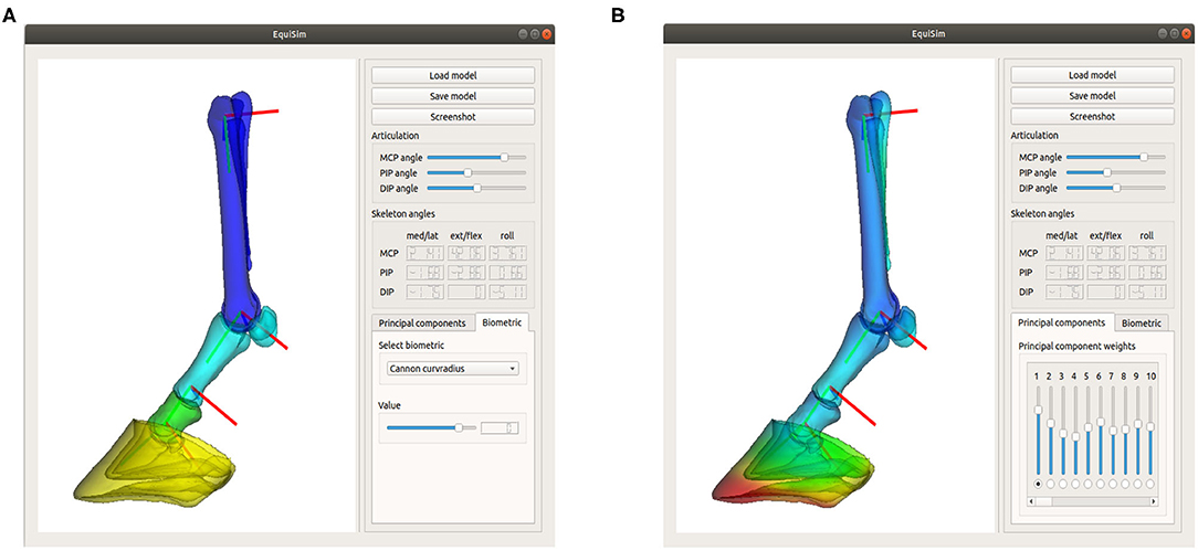
Figure 7. Screenshot of the graphical user interface “Equisim,” which allows the user to interact easily with the model, by either changing the biometric values (A) or by directly changing the PC weights (B).

Although the resulting model has been shown to be a compact representation of the population, there are still some limitations that can be a starting point for future research. First, the dataset of equine limbs collected for this proof-of-concept study was ill-controlled, combining different breeds, ages, levels of hoof conditions, etc. This maximized the sample size, but at the same time, made it less relevant for morphological studies. Depending on the target application, it would be beneficial to build a model from a specific dataset.

Second, the authors recommend basic hoof trimming and cleaning prior to the data acquisition. The poor hoof conditions in our collection of limbs caused ambiguities in the data segmentation and most likely also affected the segmentation accuracy, besides the reported registration accuracy. This subsequently can lead to irrelevant variation modes in the SSM. Similarly, bone ossification between MC 3 and MC 2 or between MC 3 and MC 4 (splints) also posed difficulties in the segmentation of both metacarpals in some cases.

Besides the data preparation, the model has some more theoretical limitations. The model is not a statistical shape and pose model, in the sense that the pose variations are not statistically described. In this paper, the pose of the model is altered based on a mathematical model, which does not correlate with the shape instance. Changing PC weights does not affect the range of motion. This limitation is due to the difficulty to acquire geometry data in different poses, preferably in vivo.

Furthermore, the model is a surface model and not a volumetric model. In order to apply our model for finite element analyses (43), one still needs to extend the model to a voxelized or tetrahedral model and assign material properties to its cells. The shape variability of our model would enable easy repetitions of the FE analysis for different shape instances. Changing only one biometric allows to study the effect of it on a particular FE result. For kinematical studies, the model can possibly be extended to a musculoskeletal model by transferring muscle, tendon, and ligament attachments from the 3D Horse Anatomy of Biosphera software (3, 44).

The main purpose of the model, as presented in this paper, lies in the compact description of the bones statistical variability. This geometric information can be exploited in CAD of different types of orthopaedic implants, suiting different classes of bone shapes. The ability to create different instances of the SSM also enables the generation of extensive training databases for deep learning applications. Digital or after 3D printing, the model can potentially have educational purposes as well.

5. Conclusion

In this paper, we presented a workflow to build an articulating statistical shape model of the equine distal limb, as a way to describe its morphological variations in a compact representation. 3D shape variations have been related to common one-dimensional biometrics. We thereby bridged the gap between current morphology studies and future digitalizations in veterinary research. Being available through an open-source application, our model can be an added value in veterinary anatomy classes and can potentially support future research in CADs, finite element analyses, and deep learning-based solutions for image processing tasks.

Data Availability Statement

The statistical model and GUI presented in this study can be found on the github repository: https://github.com/jvhoutte/equisim.

Ethics Statement

Ethical review and approval was not required for the animal study because the collection of equine limbs was donated by a commercial abattoir. The animals were slaughtered for reasons unrelated to this study. Because of the nature of the samples, no additional ethical approval was required for this study. Written informed consent for participation was not obtained from the owners because the livestock animals were slaughtered at the commercial abattoir and samples were donated post-mortem. The samples were anonymized before they got delivered to the researchers.

Author Contributions

All authors were involved in the study design. FV was responsible for the experimental part of the study and the data-collection of the CT-data. The theoretical part of the study design was outlined by JS, TH, GZ, and JV. The data analysis and the development of the GUI was performed by JV.

Funding

This work was supported by the Research Foundation in Flanders (FWO-SB 1S63918N).

Conflict of Interest

The authors declare that the research was conducted in the absence of any commercial or financial relationships that could be construed as a potential conflict of interest.

Acknowledgments

The authors would like to thank the equine hospital Bosdreef for the CT acquisitions, Denise Vogel for the storage of the cadaver equine limbs, and Julie Delhem for her contribution to the CT segmentation corrections.

Footnote

1. ^https://github.com/jvhoutte/equisim

References

1. Zarucco L, Wisner ER, Swanstrom MD, Stover SM. Image fusion of computed tomographic and magnetic resonance images for the development of a three-dimensional musculoskeletal model of the equine forelimb. Vet Radiol Ultrasound. (2006) 47:553–62. doi: 10.1111/j.1740-8261.2006.00185.x

PubMed Abstract | CrossRef Full Text | Google Scholar

2. Harrison SM, Whitton RC, Kawcak CE, Stover SM, Pandy MG. Relationship between muscle forces, joint loading and utilization of elastic strain energy in equine locomotion. J Exp Biol. (2010) 213:3998–4009. doi: 10.1242/jeb.044545

PubMed Abstract | CrossRef Full Text | Google Scholar

3. Becker J, Emmanuel M, Jean-Marc L. Joint loading estimation method for horse forelimb high jerk locomotion: jumping. J Bionic Eng. (2019) 16:674–85. doi: 10.1007/s42235-019-0054-z

CrossRef Full Text | Google Scholar

4. Mouloodi S, Rahmanpanah H, Burvill C, Davies HM. Accuracy quantification of the reverse engineering and high-order finite element analysis of equine MC3 forelimb. J Equine Vet Sci. (2019) 78:94–106. doi: 10.1016/j.jevs.2019.04.004

PubMed Abstract | CrossRef Full Text | Google Scholar

5. Lee S, Lee J, Lee A, Park N, Song S, Seo A, et al. Augmented reality intravenous injection simulator based 3D medical imaging for veterinary medicine. Vet J. (2013) 196:197–202. doi: 10.1016/j.tvjl.2012.09.015

PubMed Abstract | CrossRef Full Text | Google Scholar

6. Van Houtte J, Bazrafkan S, Vandenberghe F, Zheng G, Sijbers J. A deep learning approach to horse bone segmentation from digitally reconstructed radiographs. In: 2019 Ninth International Conference on Image Processing Theory, Tools and Applications (IPTA). (2019). p. 1–6. doi: 10.1109/IPTA.2019.8936082

CrossRef Full Text | Google Scholar

7. Dzierzçka M, Purzyc H, Charuta A, Barszcz K, Komosa M, Hecold M, et al. Evaluation of distal phalanx formation and association with front hoof conformation in coldblooded horses. Biologia. (2016) 71:337–42. doi: 10.1515/biolog-2016-0037

CrossRef Full Text | Google Scholar

8. Faramarzi B, McMicking H, Halland S, Kaneps A, Dobson H. Incidence of palmar process fractures of the distal phalanx and association with front hoof conformation in foals. Equine Vet J. (2015) 47:675–9. doi: 10.1111/evj.12375

PubMed Abstract | CrossRef Full Text | Google Scholar

9. Faramarzi B, Kepler A, Dong F, Dobson H. Morphovolumetric analysis of the hoof in standardbred horses. J Equine Vet Sci. (2018) 71:40–5. doi: 10.1016/j.jevs.2018.08.012

CrossRef Full Text | Google Scholar

10. Souza A, Kunz J, Laus R, Moreira M, Muller T, Fonteque J. Biometrics of hoof balance in equids. Arquivo Brasil Med Vet Zoot. (2016) 68:825–31. doi: 10.1590/1678-4162-8848

CrossRef Full Text | Google Scholar

11. Sampaio BFB, Zúccari CESN, Shiroma MYM, Bertozzo BR, Leonel ECR, Surjus RdS, et al. Biometric hoof evaluation of athletic horses of show jumping, barrel, long rope and polo modalities. Rev Brasil Saúde Prod Anim. (2013) 14:448–59. doi: 10.1590/S1519-99402013000300017

CrossRef Full Text | Google Scholar

12. Alrtib A, Philip C, Abdunnabi A, Davies H. Morphometrical study of bony elements of the forelimb fetlock joints in horses. Anat Histol Embryol. (2013) 42:9–20. doi: 10.1111/j.1439-0264.2012.01158.x

PubMed Abstract | CrossRef Full Text | Google Scholar

13. Cootes TF, Taylor CJ, Cooper DH, Graham J. Active shape models-their training and application. Comput Vis Image Understand. (1995) 61:38–59. doi: 10.1006/cviu.1995.1004

CrossRef Full Text | Google Scholar

14. Audenaert EA, Van Houcke J, Almeida DF, Paelinck L, Peiffer M, Steenackers G, et al. Cascaded statistical shape model based segmentation of the full lower limb in CT. Comput Methods Biomech Biomed Eng. (2019) 22:644–57. doi: 10.1080/10255842.2019.1577828

PubMed Abstract | CrossRef Full Text | Google Scholar

15. Kainmueller D, Lamecker H, Zachow S, Hege HC. An articulated statistical shape model for accurate hip joint segmentation. In: 2009 Annual International Conference of the IEEE Engineering in Medicine and Biology Society. Minneapolis, MN (2009). p. 6345–51. doi: 10.1109/IEMBS.2009.5333269

CrossRef Full Text | Google Scholar

16. Zheng G, Dong X, Rajamani KT, Zhang X, Styner M, Thoranaghatte RU, et al. Accurate and robust reconstruction of a surface model of the proximal femur from sparse-point data and a dense-point distribution model for surgical navigation. IEEE Trans Biomed Eng. (2007) 54:2109–22. doi: 10.1109/TBME.2007.895736

PubMed Abstract | CrossRef Full Text | Google Scholar

17. Balestra S, Schumann S, Heverhagen J, Nolte L, Zheng G. Articulated statistical shape model-based 2D-3D reconstruction of a hip joint. In: Lecture Notes in Computer Science (including subseries Lecture Notes in Artificial Intelligence and Lecture Notes in Bioinformatics), Vol. 8498. Fukuoka (2014). doi: 10.1007/978-3-319-07521-1_14

CrossRef Full Text | Google Scholar

18. Zheng G, Yu W. Statistical shape and deformation models based 2D-3D reconstruction. In: Zheng G, Li S, Székely G, editors. Statistical Shape and Deformation Analysis. Amsterdam: Elsevier (2017). p. 329–49. doi: 10.1016/B978-0-12-810493-4.00015-8

CrossRef Full Text | Google Scholar

19. Campbell J, Petrella A. Automated finite element modeling of the lumbar spine: using a statistical shape model to generate a virtual population of models. J Biomech. (2016) 49:2593–9. doi: 10.1016/j.jbiomech.2016.05.013

PubMed Abstract | CrossRef Full Text | Google Scholar

20. Väänänen SP, Grassi L, Flivik G, Jurvelin JS, Isaksson H. Generation of 3D shape, density, cortical thickness and finite element mesh of proximal femur from a DXA image. Med Image Anal. (2015) 24:125–34. doi: 10.1016/j.media.2015.06.001

PubMed Abstract | CrossRef Full Text | Google Scholar

21. Cerveri P, Belfatto A, Baroni G, Manzotti A. Stacked sparse autoencoder networks and statistical shape models for automatic staging of distal femur trochlear dysplasia. Int J Med Robot Comput Assist Surg. (2018) 14:e1947. doi: 10.1002/rcs.1947

PubMed Abstract | CrossRef Full Text | Google Scholar

22. Fitzpatrick CK, Baldwin MA, Laz PJ, FitzPatrick DP, Lerner AL, Rullkoetter PJ. Development of a statistical shape model of the patellofemoral joint for investigating relationships between shape and function. J Biomech. (2011) 44:2446–52. doi: 10.1016/j.jbiomech.2011.06.025

PubMed Abstract | CrossRef Full Text | Google Scholar

23. Hespel AM, Wilhite R, Hudson J. Invited review-applications for 3D printers in veterinary medicine. Vet Radiol Ultrasound. (2014) 55:347–58. doi: 10.1111/vru.12176

PubMed Abstract | CrossRef Full Text | Google Scholar

24. Brinkschulte M, Bienert-Zeit A, Lüpke M, Hellige M, Staszyk C, Ohnesorge B. Using semi-automated segmentation of computed tomography datasets for three-dimensional visualization and volume measurements of equine paranasal sinuses. Vet Radiol Ultrasound. (2013) 54:582–90. doi: 10.1111/vru.12080

PubMed Abstract | CrossRef Full Text | Google Scholar

25. Lima LFSd, Barros AJBPd, Martini AdC, Stocco MB, Kuczmarski AH, Souza RLd. Photogrammetry and 3D prototyping: a low-cost resource for training in veterinary orthopedics. Ciência Rural. (2019) 49. doi: 10.1590/0103-8478cr20180929

CrossRef Full Text | Google Scholar

26. Kozic N, Weber S, Büchler P, Lutz C, Reimers N, Ballester MÁG, et al. Optimisation of orthopaedic implant design using statistical shape space analysis based on level sets. Med Image Anal. (2010) 14:265–75. doi: 10.1016/j.media.2010.02.008

PubMed Abstract | CrossRef Full Text | Google Scholar

27. Tkany L, Hofstätter B, Petersik A, Miehling J, Wartzack S, Sesselmann S. New design process for anatomically enhanced osteosynthesis plates. J Orthop Res. (2019) 37:1508–17. doi: 10.1002/jor.24299

PubMed Abstract | CrossRef Full Text | Google Scholar

28. Liley H, Zhang J, Firth EC, Fernandez JW, Besier TF. Statistical modeling of the equine third metacarpal bone incorporating morphology and bone mineral density. PLoS ONE. (2018) 13:e194406. doi: 10.1371/journal.pone.0194406

PubMed Abstract | CrossRef Full Text | Google Scholar

29. Wilson A, Agass R, Vaux S, Sherlock E, Day P, Pfau T, et al. Foot placement of the equine forelimb: relationship between foot conformation, foot placement and movement asymmetry. Equine Vet J. (2016) 48:90–6. doi: 10.1111/evj.12378

PubMed Abstract | CrossRef Full Text | Google Scholar

30. Chateau H, Degueurce C, Jerbi H, Crevier-Denoix N, Pourcelot P, Audigié F, et al. Normal three-dimensional behaviour of the metacarpophalangeal joint and the effect of uneven foot bearing. Equine Vet J. (2001) 33:84–8. doi: 10.1111/j.2042-3306.2001.tb05366.x

PubMed Abstract | CrossRef Full Text | Google Scholar

31. Joostens Z, Evrard L, Busoni V. Unipodal stance influences radiographic evaluation of foot balance in horses. Vet Radiol Ultrasound. (2019) 60:273–9. doi: 10.1111/vru.12729

PubMed Abstract | CrossRef Full Text | Google Scholar

32. Krčah M, Székely G, Blanc R. Fully automatic and fast segmentation of the femur bone from 3D-CT images with no shape prior. In: 2011 IEEE International Symposium on Biomedical Imaging: From Nano to Macro. Chicago, IL (2011). p. 2087–90.

Google Scholar

33. Grothausmann R, Beare R, Gout J, Kühnel M. Providing values of adjacent voxel with vtkDiscreteMarchingCubes. VTK J. (2016) 975. Available online at: http://hdl.handle.net/10380/3559

Google Scholar

34. Valette S, Chassery JM, Prost R. Generic remeshing of 3D triangular meshes with metric-dependent discrete Voronoi diagrams. IEEE Trans Visual Comput Graph. (2008) 14:369–81. doi: 10.1109/TVCG.2007.70430

PubMed Abstract | CrossRef Full Text | Google Scholar

35. Attene M. A lightweight approach to repairing digitized polygon meshes. Vis Comput. (2010) 26:1393–406. doi: 10.1007/s00371-010-0416-3

CrossRef Full Text | Google Scholar

36. McGuigan MP, Wilson AM. The effect of gait and digital flexor muscle activation on limb compliance in the forelimb of the horse Equus caballus. J Exp Biol. (2003) 206:1325–36. doi: 10.1242/jeb.00254

PubMed Abstract | CrossRef Full Text | Google Scholar

37. Panagiotopoulou O, Rankin JW, Gatesy SM, Hutchinson JR. A preliminary case study of the effect of shoe-wearing on the biomechanics of a horse's foot. PeerJ. (2016) 4:e2164. doi: 10.7717/peerj.2164

PubMed Abstract | CrossRef Full Text | Google Scholar

38. Merritt JS, Davies H, Burvill C, Pandy MG. Influence of muscle-tendon wrapping on calculations of joint reaction forces in the equine distal forelimb. BioMed Res Int. (2008) 2008:165730. doi: 10.1155/2008/165730

PubMed Abstract | CrossRef Full Text | Google Scholar

39. Danckaers F, Huysmans T, Lacko D, Ledda A, Verwulgen S, Van Dongen S, et al. Correspondence preserving elastic surface registration with shape model prior. In: 2014 22nd International Conference on Pattern Recognition. Stockholm (2014). p. 2143–8. doi: 10.1109/ICPR.2014.373

CrossRef Full Text | Google Scholar

40. Fletcher PT, Lu C, Pizer SM, Joshi S. Principal geodesic analysis for the study of nonlinear statistics of shape. IEEE Trans Med Imag. (2004) 23:995–1005. doi: 10.1109/TMI.2004.831793

CrossRef Full Text | Google Scholar

41. Davies RH, Twining CJ, Cootes TF, Waterton JC, Taylor CJ. A minimum description length approach to statistical shape modeling. IEEE Trans Med Imag. (2002) 21:525–37. doi: 10.1109/TMI.2002.1009388

PubMed Abstract | CrossRef Full Text | Google Scholar

42. Su Z. Statistical Shape Modelling: Automatic Shape Model Building. London, UK: University College London (2011).

Google Scholar

43. McClinchey H, Thomason J, Jofriet J. Isolating the effects of equine hoof shape measurements on capsule strain with finite element analysis. Vet Compar Orthop Traumatol. (2003) 16:67–75. doi: 10.1055/s-0038-1632762

CrossRef Full Text | Google Scholar

44. Zsoldos R, Groesel M, Kotschwar A, Kotschwar A, Licka T, Peham C. A preliminary modelling study on the equine cervical spine with inverse kinematics at walk. Equine Vet J. (2010) 42:516–22. doi: 10.1111/j.2042-3306.2010.00265.x

PubMed Abstract | CrossRef Full Text | Google Scholar